Quasilinear problems involving a perturbation with …1Département de Mathématiques, Ecole Normale...

Quasilinear problems involvinga perturbation with quadratic growth in the gradient

and a noncoercive zeroth order term

Boussad Hamour 1 & François Murat 2

Abstract

In this paper we consider the problemu ∈ H1

0 (Ω),

−div (A(x)Du) = H(x, u,Du) + f(x) + a0(x)u in D′(Ω),

where Ω is an open bounded set of RN , N ≥ 3, A(x) is a coercive matrix with coefficients inL∞(Ω), H(x, s, ξ) is a Carathéodory function which satisfies for some γ > 0

−c0A(x) ξξ ≤ H(x, s, ξ) sign(s) ≤ γ A(x) ξξ a.e. x ∈ Ω, ∀s ∈ R, ∀ξ ∈ RN ,

f belongs to LN/2(Ω) and a0 ≥ 0 to Lq(Ω), q > N/2. For f and a0 sufficiently small, we provethe existence of at least one solution u of this problem which is moreover such that eδ0|u| − 1belongs to H1

0 (Ω) for some δ0 ≥ γ and satisfies an a priori estimate.

Résumé

Dans cet article nous étudions le problèmeu ∈ H1

0 (Ω),

−div (A(x)Du) = H(x, u,Du) + f(x) + a0(x)u dans D′(Ω),

où Ω est un ouvert borné de RN , N ≥ 3, A(x) est une matrice coercive à coefficients L∞(Ω),H(x, s, ξ) est une fonction de Carathédory qui satisfait pour un certain γ > 0

−c0A(x) ξξ ≤ H(x, s, ξ) sign(s) ≤ γ A(x) ξξ p.p. x ∈ Ω, ∀s ∈ R, ∀ξ ∈ RN ,

f appartient à LN/2(Ω) et a0 ≥ 0 à Lq(Ω), q > N/2. Pour f et a0 suffisamment petits,nous démontrons qu’il existe au moins une solution u de ce problème qui est de plus telle queeδ0|u| − 1 appartient à H1

0 (Ω) pour un certain δ0 ≥ γ et satisfait une estimation a priori.

1Département de Mathématiques, Ecole Normale Supérieure, Boîte postale 92, Vieux Kouba, 16050 Alger,Algérie; e-mail: [email protected]

2Laboratoire Jacques-Louis Lions, Université Pierre et Marie Curie (Paris VI) et CNRS, Boîte courrier 187,75252 Paris Cedex 05, France; e-mail: [email protected]

1

arX

iv:1

510.

0465

3v1

[m

ath.

AP]

15

Oct

201

5

B. Hamour and F. Murat

1 IntroductionIn this paper, we consider the quasilinear problem u ∈ H1

0 (Ω),

−div (A(x)Du) = H(x, u,Du) + f(x) + a0(x)u in D′(Ω),(1.1)

where Ω is a bounded open set of RN, N ≥ 3, where A is a coercive matrix with bounded measurablecoefficients, where H(x, s, ξ) is a Carathéodory function wich has quadratic growth in ξ, and moreprecisely which satisfies for some γ > 0 and c0 ≥ 0

− c0A(x) ξξ ≤ H(x, s, ξ) sign(s) ≤ γ A(x) ξξ, a.e. x ∈ Ω, ∀s ∈ R, ∀ξ ∈ RN , (1.2)

where f ∈ LN/2(Ω), f 6= 0, and where a0 ∈ Lq(Ω), q > N2 , with

a0 ≥ 0, a0 6= 0. (1.3)

When f and a0 are sufficiently small (and more precisely when f and a0 satisfy the two smallnessconditions (2.14) and (2.15), we prove in the present paper that problem (1.1) has a least onesolution, which is moreover such that

eδ0|u| − 1 ∈ H10 (Ω), (1.4)

with ∥∥∥∥eδ0|u| − 1

δ0

∥∥∥∥H1

0 (Ω)

≤ Zδ0 , (1.5)

where δ0 ≥ γ and Zδ0 are two constants which depend only on the data of the problem (see (6.16),(6.17), (6.18) for the definitions of δ0 and Zδ0).

The main originality of our result is the fact that we assume that a0 satisfies (1.3), namely thata0 is a nonnegative function.

Let us begin with some review of the literature.Problem (1.1) has been studied in many papers in the case where a0 ≤ 0. Among these papers

is a series of papers [8], [9], [10] and [11] by L. Boccardo, F. Murat and J.-P. Puel (see also thepaper [23] by J.-M. Rokotoson), which are concerned with the case where

a0(x) ≤ −α0 < 0. (1.6)

In these papers (which also consider nonlinear monotone operators and not only the linear operator−div (A(x)Du), the authors prove that when a0 satisfies (1.6) and when f belongs to Lq(Ω), q > N

2 ,then there exists at least one solution of (1.1) which moreover belongs to L∞(Ω) and which satisfiessome a priori estimates. The uniqueness of such a solution has been proved, under some furtherstructure assumptions, by G. Barles and F. Murat in [4], by G. Barles, A.-P. Blanc, C. Georgelinand M. Kobylanski in [3] and by G. Barles and A. Porretta in [5].

2

Quasilinear problems with a noncoercive zeroth order term

The case wherea0 = 0 (1.7)

was considered, among others, by A. Alvino, P.-L. Lions and G. Trombetti in [1], by C. Maderna,C. Pagani and S. Salsa in [21], by V. Ferone and M.-R. Posteraro in [16], and by N. Grenon-Isselkouand J. Mossino in [17]. In these papers (which also consider nonlinear monotone operators), theauthors prove that when a0 satisfies (1.7) and when f belongs to Lq(Ω), q > N

2 , with ‖f‖Lq(Ω)

sufficiently small, then there exists at least one solution of (1.1) which moreover belongs to L∞(Ω)and which satisfies some a priori estimates.

The case where a0 satisfies (1.7) but where f only belongs to LN/2(Ω) for N ≥ 3 (and nomore to Lq(Ω) with q > N

2 ) was considered by V. Ferone and F. Murat in [13] (and in [14] in thenonlinear monotone case). These authors proved that when ‖f‖LN/2(Ω) is sufficiently small, thereexists at least one solution of (1.1) which is moreover such that eδ|u| − 1 ∈ H1

0 (Ω) for some δ > γ,and that such a solution satisfies an a priori estimate. Similar results were obtained in the casewhere f ∈ LN/2(Ω) by A. Dall’Aglio, D. Giachetti and J.-P. Puel in [12] for possibly unboundeddomains when a0 satisfies (1.6); in this case no smallness condition is required on f . Finally, in [15],V. Ferone and F. Murat considered (also in the case of nonlinear monotone operators) the casewhere a0 satisfies a0 ≤ 0 and where f belongs to the Lorentz space LN/2,∞(Ω); in this case twosmallness conditions should be fulfilled.

To finish with the case where a0 satisfies a0 ≤ 0, let us quote the paper [22] by A. Porretta,where the author studies the asymptotic behaviour of the solution u of (1.1) when a0 is a strictlypositive constant which tends to zero, and proves that an ergodic constant appears at the limita0 = 0. Let us also mention the case where the nonlinearity H(x, s, ξ) has the “good sign property”,namely satisfies

−H(x, s, ξ) sign (s) ≥ 0. (1.8)

In this case, when a0 ≤ 0 and when f belongs to H−1(Ω), L. Boccardo, F. Murat and J.-P. Puelin [7] and A. Bensoussan, L. Boccardo and F. Murat in [6] proved the existence of at least onesolution of (1.1) which belongs to H1

0 (Ω).

In contrast with the cases (1.6) and (1.7), the present paper is concerned with the case (1.3)where a0 ≥ 0 and a0 6= 0.

In this setting we are only aware of four papers, which are recent. In [20], L. Jeanjean andB. Sirakov proved the existence of at least two solutions of (1.1) (which moreover belong to L∞(Ω))when A(x) = Id, H(x, s, ξ) = µ|ξ|2, µ > 0, f ∈ Lq(Ω), q > N

2 , f ≥ 0, and a0 ∈ Lq(Ω), a0 ≥ 0,a0 6= 0, with ‖f‖Lq(Ω) and ‖a0‖Lq(Ω) sufficiently small. In [2], D. Arcoya, C. De Coster, L. Jeanjeanand K. Tanaka proved the existence of a continuum (u, λ) of solutions (with u which moreoverbelongs to L∞(Ω)) when A(x) = Id, H(x, s, ξ) = µ(x) |ξ|2, with µ ∈ L∞(Ω) , µ(x) ≥ µ > 0,f ∈ Lq(Ω), q > N

2 , f ≥ 0, f 6= 0 and a0(x) = λa?0(x) with a?0 ∈ Lq(Ω), a?0 ≥ 0 and a?0 6= 0;moreover, under some further conditions on f , these authors proved that this continuum is definedfor λ ∈] − ∞ , λ0] with λ0 > 0, and that there are at least two nonnegative solutions of (1.1)when λ > 0 is sufficiently small. In [24], in a similar setting, assuming only that µ(x) ≥ 0but that the supports of µ and of a?0 have a nonempty intersection and that N ≤ 5, P. Soupletproved the existence of a continuum (u, λ) of solutions, and that there are at least two nonnegativesolutions of (1.1) when λ > 0 is sufficiently small. In [19], L. Jeanjean and H. Ramos Quoirinproved the existence of two positive solutions (which moreover belong to L∞(Ω)) when A(x) = Id,

3


H(x, s, ξ) = µ|ξ|2, µ > 0, f ∈ Lq(Ω), q > N2 , f ≥ 0, f 6= 0, and a0 ∈ C(Ω) which can change sign

with a+0 6= 0 and which satisfies the so called “thick zero set condition”, when the first eigenvalue

of the operator −∆− (a0 + µf) in H10 (Ω) is positive.

With respect to the results obtained in the four latest papers, we prove in the present paper,as said above, the existence of (only) one solution of (1.1) in the case (1.3) (a0 ≥ 0) when a0 andf satisfy the two smallness conditions (2.14) and (2.15), but our result is obtained in the generalcase of a nonlinearity H(x, s, ξ) which satisfies only (1.2), with f ∈ LN/2(Ω) and with a0 ∈ Lq(Ω),q > N

2 . Moreover, the method which allows us to prove this result continues mutatis mutandis towork in the nonlinear monotone case where the linear operator −div (A(x)Du) is replaced by aLeray-Lions operator −div (a(x, u,Du)) working in W 1,p

0 (Ω), for some 1 < p < N , and where thequasilinear term H(x, u,Du) has p-growth in |Du|.

Let us now describe the contents of the present paper.The precise statement of our result is given in Section 2 (Theorem 2.1), as well as the precise

assumptions under which we are able to prove it. These conditions in particular include the twosmallness conditions (2.14) and (2.15).

Our method for proving Theorem 2.1 is based on an equivalence result (see Theorem 3.5) thatwe state in Section 3 once we have introduced the functions Kδ(x, s, ζ) and gδ(s) (see (3.6) and(3.7)) and made some technical remarks on them. This result is very close to the equivalence resultgiven in the paper [14] by V. Ferone and F. Murat.

This equivalence result implies that in order to prove the existence of a solution u of (1.1) whichsatisfies (1.4) and (1.5), it is equivalent to prove (see Theorem 3.8) the existence of a function wdefined by (3.31), i.e.

w =1

δ0(eδ0|u| − 1) sign(u), (1.9)

which satisfies (3.33), i.e.w ∈ H1

0 (Ω),

−div(A(x)Dw) +Kδ0(x,w,Dw) sign(w) =

= (1 + δ0|w|) f(x) + a0(x)w + a0(x) gδ0(w) sign(w) in D′(Ω),

(1.10)

and the estimate (3.34), i.e.‖w‖H1

0 (Ω) ≤ Zδ0 , (1.11)

(which is nothing but (1.5)).Our goal thus becomes to prove Theorem 3.8, namely to prove the existence of a solution w

which satisfies (1.10) and (1.11).Problem (1.10) is very similar to problem (1.1), since it involves a term −Kδ0(x,w,Dw) sign(w)

which has quadratic growth in Dw, as well as a zeroth order term δ0 |w|f(x) ++ a0(x)w + a0(x) gδ0(w) sign(w). But this problem is also very different from (1.1), since theterm −Kδ0(x,w,Dw) sign(w) with quadratic growth has now the “good sign property” (see (1.8)),

4


since Kδ0(x, s, ξ) satisfiesKδ0(x, s, ξ) ≥ 0,

while the zeroth order term is now no more a linear but a semilinear term with |s|1+θ growth (see(6.20)) due to presence of the term a0(x) gδ0(w) sign(w).

We will prove Theorem 3.8 essentially by applying Schauder’s fixed point theorem. But thereare some difficulties to do it directly, since the term with quadratic growth Kδ0(x,w,Dw) sign(w)only belongs to L1(Ω) in general. We therefore begin by defining an approximate problem (see(4.1)) where Kδ(x,w,Dw) is remplaced by its truncation at height k, namely Tk(Kδ(x,w,Dw)),and we prove (see Theorem 4.1) that if f and a0 satisfy the two smallness conditions (2.14) and(2.15), this approximate problem has at least one solution wk which satisfies the a priori estimate

‖wk‖H10 (Ω) ≤ Zδ0 . (1.12)

This result, which is proved in Section 4, is obtained by applying Schauder’s fixed point theoremin a classical way.

We then pass to the limit as k tends to infinity and we prove in Section 5 that (for a subsequenceof k) wk tend to some w? strongly in H1

0 (Ω) (see (5.2)) and that this w? is a solution of (1.10)which also satisfies (1.11) (see End of the proof of Theorem 3.8).

This completes the proof of Theorem 3.8, and therefore proves Theorem 2.1, as announced.

This proof follows along the lines of the proof used by V. Ferone and F. Murat in [13] inthe case where a0 = 0. As mentionned above, this method can be applied mutatis mutandis tothe nonlinear case where the linear operator −div(A(x)Du) is replaced by a Leray-Lions oper-ator −div(a(x, u,Du)) working in W 1

0 (Ω) for some 1 < p < N , and where the quasilinear termH(x, u,Du) has p-growth in |Du|, as it was done in [14] by V. Ferone and F. Murat in this nonlinearsetting when a0 = 0. This will be the goal of our next paper [18].

2 Main result

In this paper we consider the following quasilinear problem u ∈ H10 (Ω),

−div (A(x)Du) = H(x, u,Du) + a0(x)u+ f(x) in D′(Ω),(2.1)

where the set Ω satisfies (note that no regularity is assumed on the boundary of Ω)

Ω is a bounded open subset of RN , N ≥ 3, (2.2)

where the matrix A is a coercive matrix with bounded measurable coefficients, i.e. A ∈ (L∞(Ω))N×N ,

∃α > 0, A(x) ξξ ≥ α|ξ|2 a.e. x ∈ Ω, ∀ξ ∈ RN ,(2.3)

5


where the function H(x, s, ξ) is a Carathéodory function with quadratic growth in ξ, and moreprecisely satisfies

H : Ω× R× RN → R is a Carathéodory function such that

−c0A(x) ξξ ≤ H(x, s, ξ) sign(s) ≤ γ A(x) ξξ, a.e. x ∈ Ω, ∀s ∈ R, ∀ξ ∈ RN ,

where γ > 0 and c0 ≥ 0,

(2.4)

where sign : R→ R denotes the function defined by

sign(s) =

+1 if s > 0,0 if s = 0,−1 if s < 0,

(2.5)

where the coefficient a0 satisfies

a0 ∈ Lq(Ω) for some q >N

2, a0 ≥ 0, a0 6= 0, (2.6)

as well as the technical assumption (note that, sinceN

2<

2N

6−Nwhen 3 ≤ N ≤ 6 and since Ω is

bounded, this assumption can be made without loss of generality once hypothesis (2.6) is assumed)

N

2< q <

2N

6−Nwhen 3 ≤ N ≤ 6, (2.7)

and finally wheref ∈ LN/2(Ω), f 6= 0. (2.8)

Since N ≥ 3, let 2∗ be the Sobolev’s exponent defined by

1

2∗=

1

2− 1

N,

and let CN be the Sobolev’s constant defined as the best constant such that

‖ϕ‖2∗ ≤ CN‖Dϕ‖2, ∀ϕ ∈ H10 (Ω). (2.9)

We claim that in view of (2.6) and (2.7), one has

0 <2∗

q′− 2 < 1, (2.10)

where q′ the Hölder’s conjugate of the exponent q, i.e.

1

q′+

1

q= 1;

6


indeed easy computations show that

0 <2∗

q′− 2 ⇐⇒ q >

N

2,

2∗

q′− 2 < 1 ⇐⇒ 1

q>

6−N2N

,

where the latest inequality is satisfied when N > 6 and is equivalent to q <2N

6−Nwhen N ≤ 6

(see (2.7)).We now define the number θ by

θ =2∗

q′− 2. (2.11)

In view of (2.10) we have0 < θ < 1. (2.12)

Since Ω is bounded, we equip the space H10 (Ω) with the norm

‖u‖H10 (Ω) = ‖Du‖L2(Ω)N . (2.13)

We finally assume that f and a0 are sufficiently small (see Remark 2.2), and more preciselythat

α− C2N‖a0‖N/2 − γC2

N‖f‖N/2 > 0, (2.14)

‖f‖H−1(Ω) ≤θ

1 + θ

(α− C2N‖a0‖N/2 − γC2

N‖f‖N/2)(1+θ)/θ

((1 + θ)GC2+θN ‖a0‖q)1/θ

, (2.15)

where the constant G is defined by (6.14).Observe that in place of (2.14) we could as well have assumed that

α− C2N‖a0‖N/2 − γC2

N‖f‖N/2 ≥ 0,

but that when equality takes places in the latest inequality, inequality (2.15) implies that f = 0,and then u = 0 is a solution of (2.1), so that the result of Theorem 2.1 becomes trivial.

Our main result is the following Theorem.

Theorem 2.1 Assume that (2.2), (2.3), (2.4), (2.6), (2.7) and (2.8) hold true. Assume moreoverthat the two smallness conditions (2.14) and (2.15) hold true.

Then there exist a constant δ0 with δ0 ≥ γ, and a constant Zδ0 , which are defined in Lemma 6.2(see (6.16), (6.17)) and (6.18)), such that there exists at least one solution u of (2.1) which furthersatisfies

(eδ0|u| − 1) ∈ H10 (Ω), (2.16)

with

‖eδ0|u|Du‖L2(Ω)N =

∥∥∥∥eδ0|u| − 1

δ0

∥∥∥∥H1

0 (Ω)

≤ Zδ0 . (2.17)

7


Our proof of Theorem 2.1 is based on an equivalence result (Theorem 3.5) which will be statedand proved in Section 3. This equivalence Theorem will allows us to replace proving Theorem 2.1by proving Theorem 3.8 which is equivalent to Theorem 2.1.

Remark 2.2 In this Remark, we consider that the open set Ω, the matrix A and the functionH are fixed (and therefore in particular that the constants α > 0 and γ > 0 are fixed), and weconsider the functions a0 and f as parameters.

Our first set of assumptions on these parameters (assumptions (2.6) and (2.7)) is that a0 belongsto Lq(Ω) with q > N

2 (and that q < 2NN−6 when 3 ≤ N ≤ 6; as said above this assumption can be

made without loss of generality). This first set of assumptions is essential to ensure (see (2.10)) thatthe exponent θ defined by (2.11) satisfies 0 < θ < 1 (see (2.12)). We also assume a0 ≥ 0 and a0 6= 0.

Our second set of assumptions on these parameters is made of the two smallness conditions(2.14) and (2.15).

Indeed, if, for example, a0 is sufficiently small such that it satisfies

α− C2N‖a0‖N/2 > 0,

then the two smallness conditions (2.14) and (2.15) are satisfied if ‖f‖N/2 (and therefore ‖f‖H−1(Ω),since LN/2(Ω) ⊂ H−1(Ω)) is sufficiently small.

Similarly, if, for example, f is sufficiently small such that it satisfies

α− γC2N‖f‖N/2 > 0,

then the two smallness conditions (2.14) and (2.15) are satisfied if ‖a0‖q is sufficiently small (whichimplies, since Lq(Ω) ⊂ LN/2(Ω), that ‖a0‖N/2 is sufficiently small), since ‖a0‖q appears in thedenominator of the right-hand side of (2.15).

Remark 2.3 The definitions of the two constants δ0 and Zδ0 which appear in Theorem 2.1 aregiven in (the technical) Appendix 6 (see Lemma 6.2). These definitions are based on the propertiesof the family of functions Φδ (see (6.13)) which look like convex parabolas (see Figure 2 andRemark 6.3): the constant δ0 is the unique value of the parameter δ for which the function Φδ0has a double zero, and Zδ0 is the value of this double zero. The two smallness conditions (2.14)and (2.15) ensure that δ0 satisfies δ0 ≥ γ, a condition which is essential in our proof.

In Remark 3.9 we try to explain where the two smallness conditions (2.14) and (2.15) comefrom.

In Remark 3.10, we explain why we have chosen to state Theorem 3.8 with δ = δ0 rather thanwith a fixed δ with γ ≤ δ ≤ δ0.

Remark 2.4 In assumption (2.2) we have assumed that N ≥ 3, because we use the Sobolev’sembedding (2.9). All the proofs of the present paper can nevertheless be easily adapted to thecases where N = 1 and N = 2, providing similar results, by using the fact that H1

0 (Ω) ⊂ L∞(Ω)when N = 1 and that H1

0 (Ω) ⊂ Lp(Ω) for every p < +∞ when N = 2, and by replacing assumption

q >N

2made in (2.6) when N ≥ 3 by q = 1 when N = 1 and by q > 1 when N = 2, and the

assumption made in (2.8) that f ∈ LN/2(Ω) by f ∈ L1(Ω) when N = 1 and by f ∈ Lm(Ω) withm > 1 when N = 2 (and also replacing the norm ‖f‖N/2 by the corresponding norm).

8


In assumption (2.6) and (2.8) we have assumed that a0 6= 0 and that f 6= 0. Indeed the casewhere a0 = 0 has been treated by V. Ferone and F. Murat in [13], and in the case where f = 0,then u = 0 is a solution of (2.1) and the results of the present paper become trivial.

3 An equivalence result

The main results of this Section are Theorems 3.5 and 3.8. In contrast, Remarks 3.1, 3.2 and 3.4and Lemma 3.3 can be considered as technical results.

Indeed, as said above, the proof of Theorem 2.1 is based on the equivalence result of Theorem3.5 that we state and prove in this Section. This equivalence Theorem in particular implies thatTheorem 3.8, which we state at the end of this Section, is equivalent to Theorem 2.1. Theorem3.8 will be proved in Sections 4 and 5.

This Section also includes Remark 3.9 in which we try to explain where the two smallnessconditions (2.14) and (2.15) come from, as well as Remark 3.10 where we explain why we havechosen to state Theorem 3.8 for δ = δ0.

In this Section (as well as in the whole of the present paper) we always assume that

δ > 0. (3.1)

Let us first proceed with a formal computation.If u is a solution of −div (A(x)Du) = H(x, u,Du) + f(x) + a0(x)u in Ω,

u = 0 on ∂Ω,(3.2)

and if we formally define the function wδ by

wδ =1

δ

(eδ|u| − 1

)sign(u), (3.3)

where the function sign is defined by (2.5), we have, at least formally,

eδ|u| = 1 + δ|wδ|, |u| = 1

δlog(1 + δ|wδ|), sign(u) = sign(wδ),

Dwδ = eδ|u|Du, A(x)Dwδ = eδ|u|A(x)Du,

−div (A(x)Dwδ) = −δeδ|u|A(x)DuDu sign(u)− eδ|u|(div (A(x)Du)

),

(3.4)

9


and therefore wδ is, at least formally, a solution of

−div (A(x)Dwδ) =

= −δeδ|u|A(x)DuDu sign(u) + eδ|u|H(x, u,Du) + eδ|u| f(x) + eδ|u| a0(x)u =

= −Kδ(x,wδ, Dwδ) sign(wδ) +

+(1 + δ|wδ|) f(x) + a0(x)wδ + a0(x) gδ (wδ) sign(wδ) in Ω,

wδ = 0 on ∂Ω,

(3.5)

whenever the functions Kδ : Ω× R× RN → R and gδ : R→ R are defined by the formulas

Kδ(x, t, ζ) =

=δ

1 + δ|t|A(x)ζζ − (1 + δ|t|)H(x,

1

δlog(1 + δ|t|) sign(t),

ζ

1 + δ|t|) sign(t),

a.e. x ∈ Ω, ∀t ∈ R, ∀ζ ∈ RN ,

(3.6)

andgδ(t) = −|t|+ 1

δ(1 + δ|t|) log(1 + δ|t|), ∀t ∈ R, (3.7)

which is equivalent to

t+ gδ(t) sign(t) = (1 + δ|t|)1

δlog(1 + δ|t|) sign(t), ∀t ∈ R. (3.8)

Conversely, if wδ is a solution of (3.5), and if we formally define the function u by

u =1

δlog(1 + δ|wδ|) sign(wδ), (3.9)

the same formal computation easily shows that u is a solution of (3.2).

The main goal of this Section is to transform this formal equivalence into a mathematical result,namely Theorem 3.5. We begin with three remarks on the functions Kδ and gδ, namely Remarks3.1, 3.2 and 3.4.

10


Remark 3.1 Observe that, because of the inequality (2.4) on the function H, and because of thecoercivity (2.3) of the matrix A, one has

(c0 + δ)A(x)ζζ ≥ c0 + δ

(1 + δ|t|)A(x)ζζ =

=δ

(1 + δ|t|)A(x)ζζ + (1 + δ|t|) c0

(1 + δ|t|)2A(x)ζζ ≥

≥ Kδ(x, t, ζ) ≥

≥ δ

(1 + δ|t|)A(x)ζζ − (1 + δ|t|) γ

(1 + δ|t|)2A(x)ζζ =

=(δ − γ)

(1 + δ|t|)A(x)ζζ ≥ −|δ − γ|A(x)ζζ,

a.e. x ∈ Ω, ∀t ∈ R, ∀ζ ∈ RN , ∀δ > 0.

(3.10)

When δ ≥ γ, this computation in particular implies that

(c0 + δ)A(x)ζζ ≥ Kδ(x, t, ζ) ≥ 0 a.e. x ∈ Ω, ∀t ∈ R, ∀ζ ∈ RN if δ ≥ γ. (3.11)

Remark 3.2 In this technical Remark we prove that the functions Kδ(x,w,Dw) andKδ(x,w,Dw) sign(w) are correctly defined and are measurable functions when w ∈ H1(Ω), andwe prove their continuity with respect to the almost everywhere convergence of w and Dw (seeLemma 3.3).

Note that the function Kδ(x, t, ζ) defined by (3.6) and the function Kδ(x, t, ζ) sign(t) are notCarathéodory functions, because their definitions involve the function sign(t), which it is not aCarathéodory function since is not continuous at t = 0. This lack of continuity in t = 0 ishowever the only obstruction for the functionsKδ(x, t, ζ) andKδ(x, t, ζ) sign(t) to be Carathéodoryfunctions, and

for every w ∈ H1(Ω),

the functions Kδ(x,w,Dw) and Kδ(x,w,Dw) sign(w) are well defined

and are measurable functions,

(3.12)

11


as it immediately results from the two formulas

Kδ(x, t, ζ) =

=δ

1 + δ|t|A(x)ζζ − (1 + δ|t|)H(x,

1


ζ

1 + δ|t|) sign(t) =

=δ

1 + δ|t|A(x)ζζ +

+ χt<0(t) (1 + δ|t|)H(x,−1

δlog(1 + δ|t|), ζ

1 + δ|t|)− χt=0(t) 0 +

− χt>0(t) (1 + δ|t|)H(x,1


1 + δ|t|),

a.e. x ∈ Ω, ∀t ∈ R, ∀ζ ∈ RN ,

(3.13)

Kδ(x, t, ζ) sign(t) =

= sign(t)δ

1 + δ|t|A(x)ζζ − (1 + δ|t|)H(x,

1


ζ

1 + δ|t|) =

= − χt<0(t)δ

1 + δ|t|A(x)ζζ + χt=0(t) 0 + χt>0(t)

δ

1 + δ|t|A(x)ζζ +

− χt<0(t) (1 + δ|t|)H(x,−1


1 + δ|t|)− χt=0(t)H(x, 0, ζ) +

− χt>0(t) (1 + δ|t|)H(x,1


1 + δ|t|),

a.e. x ∈ Ω, ∀t ∈ R, ∀ζ ∈ RN .

(3.14)

Moreover, in view of (3.10) one has

Kδ(x,w,Dw) ∈ L1(Ω), Kδ(x,w,Dw) sign(w) ∈ L1(Ω), ∀w ∈ H1(Ω), ∀δ > 0. (3.15)

One also has the following convergence result.

Lemma 3.3 Consider a sequence wn such that

wn ∈ H1(Ω), w ∈ H1(Ω), wn → w a.e. in Ω, Dwn → Dw a.e. in Ω. (3.16)

Then Kδ(x,wn, Dwn)→ Kδ(x,w,Dw) a.e. in Ω,

Kδ(x,wn, Dwn) sign(wn)→ Kδ(x,w,Dw) sign(w) a.e. in Ω.(3.17)

12


Proof On the first hand, we have the following almost everywhere convergences

δ

1 + δ|wn|A(x)DwnDwn →

δ

1 + δ|w|A(x)DwDw a.e. in Ω,

(1 + δ|wn|)H(x,−1

δlog(1 + δ|wn|),

Dwn1 + δ|wn|

)→

→ (1 + δ|w|)H(x,−1

δlog(1 + δ|w|), Dw

1 + δ|w|) a.e. in Ω,

H(x, 0, Dwn)→ H(x, 0, Dw) a.e. in Ω,

(1 + δ|wn|)H(x,1

δlog(1 + δ|wn|),

Dwn1 + δ|wn|

)→

→ (1 + δ|w|)H(x,1

δlog(1 + δ|w|), Dw

1 + δ|w|) a.e. in Ω.

(3.18)

On the other hand, for almost every x fixed in the set y ∈ Ω : w(y) > 0, the assertionwn(x)→ w(x) implies, since w(x) > 0, that one has wn(x) > 0 for n sufficiently large (dependingon x), and therefore that, for some n > n?(x), one has

χwn<0(wn(x)) = 0 = χw<0(w(x)) for n > n?(x),

χwn=0(wn(x)) = 0 = χw=0(w(x)) for n > n?(x),

χwn>0(wn(x)) = 1 = χw>0(w(x)) for n > n?(x).

(3.19)

These convergences and (3.18) imply that Kδ(x,wn, Dwn)→ Kδ(x,w,Dw) a.e. in y ∈ Ω : w(y) > 0,

Kδ(x,wn, Dwn) sign(wn)→ Kδ(x,w,Dw) sign(w) a.e. in y ∈ Ω : w(y) > 0.

The same proof gives the similar result in the set y ∈ Ω : w(y) < 0.

The proof in the set y ∈ Ω : w(y) = 0 is a little bit more delicate. Let us first observe thatfor w ∈ H1(Ω) one has

Dw = 0 a.e. in y ∈ Ω : w(y) = 0, (3.20)

and since inequality (2.4) on the function H implies that

H(x, s, 0) = 0 a.e. x ∈ Ω, ∀s ∈ R, s 6= 0, (3.21)

and therefore by continuity in s that

H(x, 0, 0) = 0 a.e. x ∈ Ω. (3.22)

Then, on the first hand, theses results and formulas (3.13) and (3.14) imply that

Kδ(x,w,Dw) = Kδ(x,w,Dw) sign(w) = 0 a.e. in y ∈ Ω : w(y) = 0. (3.23)

13


On the other hand, in view of (3.20) and (3.22), the four functions which appear in the four limitsin (3.18) vanish almost everywhere in the set y ∈ Ω : w(y) = 0. Even if we do not know anythingabout the pointwise limits of the functions χwn<0(wn(x)), χwn=0(wn(x)) and χwn>0(wn(x))in the set y ∈ Ω : w(y) = 0, this fact and formulas (3.13) and (3.14) prove that Kδ(x,wn, Dwn)→ 0 a.e. in y ∈ Ω : w(y) = 0,

Kδ(x,wn, Dwn) sign(wn)→ 0 a.e. in y ∈ Ω : w(y) = 0.(3.24)

From (3.23) and (3.24) we deduce that Kδ(x,wn, Dwn)→ Kδ(x,w,Dw) a.e. in y ∈ Ω : w(y) = 0,

Kδ(x,wn, Dwn) sign(wn)→ Kδ(x,w,Dw) sign(w) a.e. in y ∈ Ω : w(y) = 0.(3.25)

This completes the proof of (3.17).

Remark 3.4 Observe that the function gδ(s) sign(s) is a Carathéodory function since in view of(6.4) this function is continuous at s = 0. This allows one to define gδ(w) sign(w) as a measurablefunction for every w ∈ H1(Ω).

The main result of this Section is the following equivalence Theorem.

Theorem 3.5 Assume that (2.2), (2.3), (2.4), (2.6), (2.7) and (2.8) hold true, and let δ > 0 befixed. Let the functions Kδ and gδ be defined by (3.6) and (3.7).

If u is any solution of (2.1) which satisfies

(eδ|u| − 1) ∈ H10 (Ω), (3.26)

then the function wδ defined by (3.3), namely by

wδ =1

δ

(eδ|u| − 1

)sign(u),

satisfies wδ ∈ H1

0 (Ω),

−div (A(x)Dwδ) +Kδ(x,wδ, Dwδ) sign(wδ) =

= (1 + δ|wδ|) f(x) + a0(x)wδ + a0(x) gδ(wδ) sign(wδ) in D′(Ω).

(3.27)

Conversely, if wδ is any solution of (3.27), then the function u defined by (3.9), namely by

u =1

δlog(1 + δ|wδ|) sign(wδ),

is a solution of (2.1) which satisfies (3.26).

14


Remark 3.6 Every term of the equation in (3.27) has a meaning in the sense of distributions:indeed the first term of the left-hand side of the equation in (3.27) belongs to H−1(Ω); on the otherhand, the four other terms of the equation are measurable functions (see Remarks 3.2 and 3.4);the second term of the left-hand side of the equation in (3.27) belongs to L1(Ω) in view of (3.10),while the three terms of the right-hand side of the equation in (3.27) can be proved to belong to(L2?(Ω))′ (see e.g. the proof of (3.40) in Remark 3.9 and the proof of (4.8) in the proof of Lemma4.2).

Remark 3.7 Observe that the equivalence Theorem 3.5 holds true without assuming the twosmallness conditions (2.14) and (2.15); moreover one could even have removed in (2.3) the assump-tion that the matrix A is coercive, and still obtain the same equivalence result.

Note however that Theorem 3.5 is an equivalence result which does not proves neither theexistence of a solution of (2.1) nor the existence of a solution of (3.27), but which assumes as anhypothesis either the existence of a solution of (2.1) which also satisfies (3.26), or the existence ofa solution of (3.27).

Proof of Theorem 3.5 Define the function f by

f(x) = f(x) + a0(x)u(x), (3.28)

In view of (3.3) and of the definition (3.7) of gδ(s), one has (see (3.8) and (3.4))

(1 + δ|wδ|) f(x) + a0(x)wδ + a0(x) gδ(wδ) sign(wδ) =

= (1 + δ|wδ|)(f(x) + a0(x)

1

δlog(1 + δ|wδ|) sign(wδ)

)=

= (1 + δ|wδ|) (f(x) + a0(x)u(x)) = (1 + δ|wδ|)f(x).

(3.29)

Then Theorem 3.5 becomes an immediate application of Proposition 1.8 of [13], once oneobserves that

f ∈ LN/2(Ω); (3.30)

such is the case in the setting of Theorem 3.5: indeed f = f + a0u, where f belongs to LN/2(Ω)by assumption (2.8), and where a0u also belongs to LN/2(Ω), since a0 is assumed to belong toLq(Ω), q > N

2 (see assumption (2.6)), while u belongs to Lr(Ω) for every r < +∞, since by (3.26)(eδ|u| − 1) is assumed to belong to H1

0 (Ω), hence in particular to L1(Ω), which implies that eδ|u|belongs to L1(Ω). Theorem 3.5 is therefore proved.

From the equivalence Theorem 3.5 one immediately deduces, setting

w =1

δ0(eδ0|u| − 1) sign(u) (3.31)

and equivalently

u =1

δ0log(1 + δ0|w|) sign(w), (3.32)

that Theorem 2.1 is equivalent to the following Theorem.

15


Theorem 3.8 Assume that (2.2), (2.3), (2.4), (2.6), (2.7) and (2.8) hold true. Assume moreoverthat the two smallness conditions (2.14) and (2.15) hold true.

Then there exist a constant δ0 with δ0 ≥ γ, and a constant Zδ0 , which are defined in Lemma 6.2(see (6.16), (6.17) and (6.18)), such that there exists at least one solution w of

w ∈ H10 (Ω),

−div(A(x)Dw) +Kδ0(x,w,Dw) sign(w) =

= (1 + δ0|w|) f(x) + a0(x)w + a0(x) gδ0(w) sign(w) in D′(Ω),

(3.33)

which satisfies‖w‖H1

0 (Ω) ≤ Zδ0 . (3.34)

The rest of this paper will therefore be devoted to the proof of Theorem 3.8. This will be donein two steps: first, in Section 4 we will prove the existence of a solution satisfying (3.34) for aproblem which approximates (3.33), see Theorem 4.1; second, in Section 5, we will pass to thelimit in this approximate problem and prove that for a subsequence the limit satisfies (3.33) and(3.34).

Remark 3.9 In this Remark we assume that (2.2), (2.3), (2.4), (2.6), (2.7) and (2.8) hold true.We also assume that the two smallness conditions (2.14) and (2.15) hold true, and we try to explainhow these two conditions come from an “a priori estimate” that one can obtain on the solutions of(3.27).

If wδ is any solution of (3.27), using Tk(wδ) ∈ H10 (Ω)∩L∞(Ω) as test function, where Tk : R→ R

is the usual truncation at height k defined by

Tk(s) =

−k if s ≤ −k,s if − k ≤ s ≤ +k,

+k if + k ≤ s,(3.35)

one has

∫Ω

A(x)DwδDTk(wδ) +

∫Ω

Kδ(x,wδ, Dwδ)|Tk(wδ)| =

=

∫Ω

f(x)Tk(wδ) +

∫Ω

δf(x)|wδ|Tk(wδ) +

∫Ω

a0(x)wδ Tk(wδ)+

+

∫Ω

a0(x) gδ(wδ) |Tk(wδ)|.

(3.36)

From now on we assume in this Remark that δ satisfies

γ ≤ δ ≤ δ1, (3.37)

where δ1 is defined by (6.11) (note that one has γ < δ1, see (6.12)).Since δ ≥ γ by (3.37), we deduce from (3.11) that Kδ(x, s, ζ) ≥ 0, and therefore that the second

term of the left-hand side of (3.36) is nonnegative. We then use in the first term of the left-handside of (3.36) the fact that the matrix A is coercive (see (2.3)), in the first term of the right-hand

16


side of (3.36) the fact that f ∈ LN/2(Ω) (see (2.8)), which implies that f ∈ H−1(Ω), in the secondand in the third terms of the right-hand side of (3.36) Hölder’s inequality with

1N2

+1

2?+

1

2?= 1,

and finally in the fourth term of the right-hand side of (3.36) the second statement of (6.19),namely

0 ≤ gδ(t) < G|t|1+θ, ∀t ∈ R, t 6= 0, ∀δ, 0 < δ ≤ δ1, (3.38)

(note that here we use δ ≤ δ1, see (3.37)) and Hölder’s inequality with

1

q+

1 + θ

2?+

1

2?= 1

(which results from the definition (2.11) of θ). This allows us to obtain an estimate on Tk(wδ), inwich we pass to the limit in k to get α‖Dwδ‖22 < ‖f‖H−1(Ω)‖Dwδ‖2 + δ‖f‖N/2‖wδ‖22? + ‖a0‖N/2‖wδ‖22? +G‖a0‖q‖wδ‖2+θ

2? ,

if wδ 6= 0,(3.39)

(note that in view of (3.38), inequality (3.39) is actually a strict inequality). Using Sobolev’sinequality (2.9) and dividing by ‖Dwδ‖2 this implies that (even in the case where wδ = 0)

α‖Dwδ‖2 < ‖f‖H−1(Ω) + δC2N‖f‖N/2 + C2

N‖a0‖N/2 +GC2+θN ‖a0‖q‖Dwδ‖1+θ

2 . (3.40)

In view of the definition (6.13) of the function Φδ (see also Figure 2), we have proved that ifwδ is any solution of (3.27), one has

Φδ(‖Dwδ‖2) > 0 if γ ≤ δ ≤ δ1. (3.41)

But by the definition of δ0, one has

Φδ(X) > 0, ∀X ≥ 0, ∀δ, 0 < δ ≤ δ1,

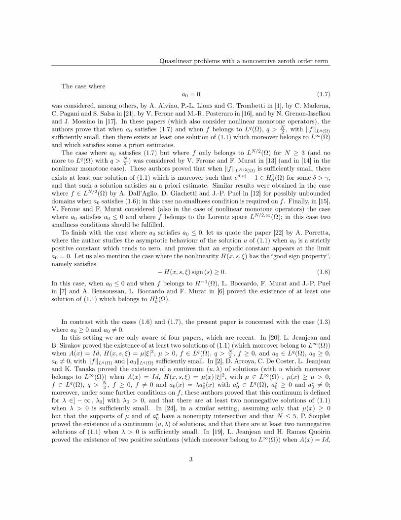
and therefore inequality (3.41) does not imply anything on ‖Dwδ‖2 when δ satisfies δ0 < δ ≤ δ1.In contrast, when δ < δ0, the strict inequality (3.41) implies that

either ‖Dwδ‖2 < Y −δ or ‖Dwδ‖2 > Y +δ if δ < δ0, (3.42)

where Y −δ < Y +δ are the two distinct zeros of the function Φδ (see Remarks 6.3 and 6.5 and

Figure 2), while when δ = δ0, the strict inequality (3.41) implies that

either ‖Dwδ0‖2 < Zδ0 or ‖Dwδ0‖2 > Zδ0 if δ = δ0. (3.43)

Inequalities (3.42) and (3.43) are not a priori estimates, since they do not imply any bound on‖Dwδ‖2. Nevertheless these inequalities exclude the closed interval [Y −δ , Y +

δ ] or the point Zδ0 for‖Dwδ‖2, and they give the hope to prove the existence of a fixed point in the set ‖Dwδ‖2 ≤ Y −δ ,when δ < δ0, or in the set ‖Dwδ0‖2 ≤ Zδ0 , when δ = δ0.

17


These inequalities also explain where the two smallness conditions (2.14) and (2.15) come from.Indeed (see Remark 6.3), these two smallness conditions imply that the value δ0 of δ for whichΦδ has a double zero satisfies δ0 ≥ γ, which is the case where, as said just above, some hope isallowed.

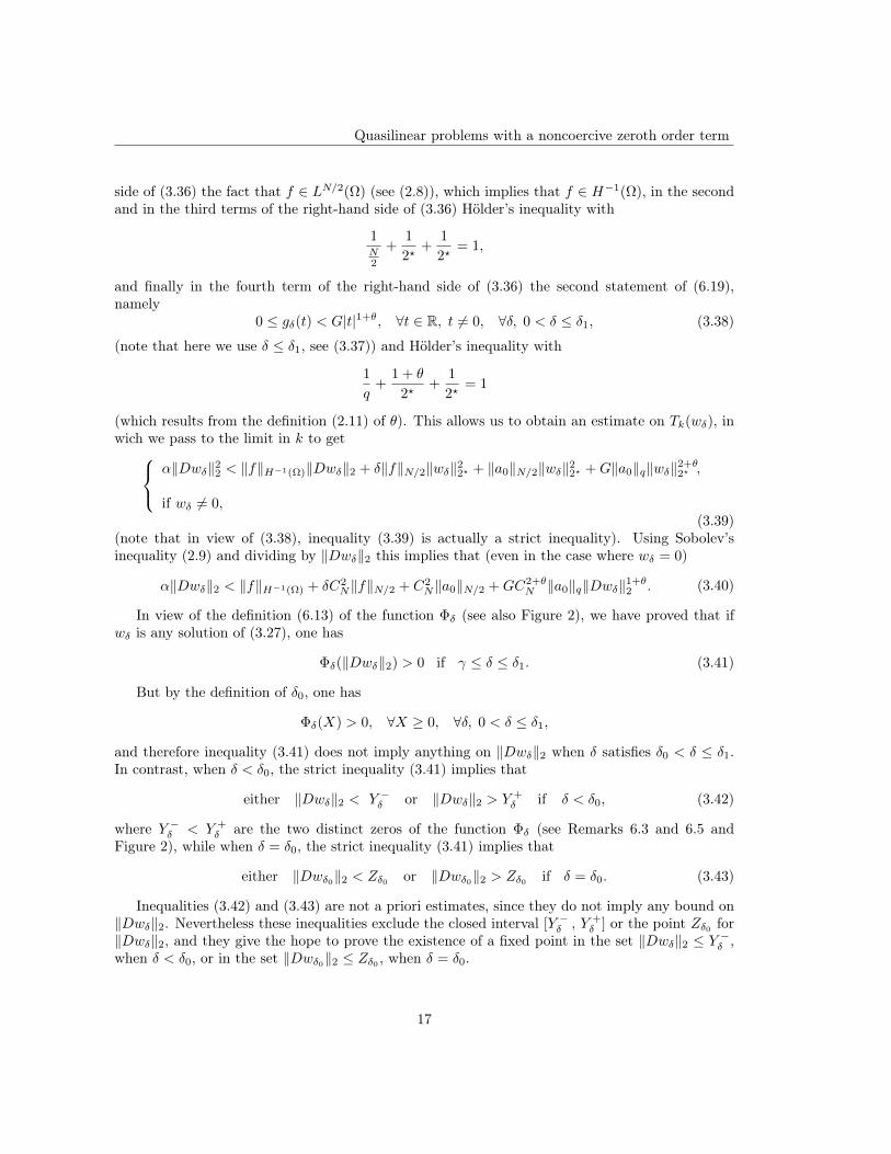
Remark 3.10 In the present paper, we have chosen to prove the existence of a function w whichis a solution of (3.33) (or in other terms of a function w = wδ0 which is a solution of (3.27) withδ = δ0) which satisfies ‖w‖H1

0 (Ω) ≤ Zδ0 (see (3.34)). When γ < δ0, i.e. when the inequality (2.15)is a strict inequality, we could as well have chosen to prove that for any fixed δ with γ ≤ δ < δ0,there exists a function wδ which is a solution of (3.27) which satisfies ‖wδ‖H1

0 (Ω) ≤ Y −δ , where Y −δis the smallest zero of the function Φδ (see Remark 6.5 and Figure 2): indeed the proofs made inSections 4 and 5 continue to work in this framework and allow one to prove this result.

In this framework, if we define, for any fixed δ with γ ≤ δ < δ0, the function uδ by

uδ =1

δlog(1 + δ|wδ|) sign(wδ) (3.44)

(compare with the definition (3.32) of u, where δ = δ0), the existence of a solution wδ of (3.27)which satisfies ‖wδ‖H1

0 (Ω) ≤ Y −δ proves (see the equivalence Theorem 3.5) that uδ defined by (3.44)is a solution of (2.1) which satisfies

‖eδ|uδ|Duδ‖2 = ‖Dwδ‖2 ≤ Y −δ .

But the function u which is defined by (3.32) from the function w given by Theorem 3.8 satisfies(2.1) (by the equivalence Theorem 3.5 with δ = δ0) and (see (3.4) again)

‖eδ0|u|Du‖2 = ‖Dw‖2 ≤ Zδ0 .

When δ < δ0, we therefore have

‖eδ|u|Du‖2 ≤ ‖eδ0|u|Du‖2 ≤ Zδ0 , if δ < δ0,

and therefore eδ|u| − 1 ∈ H10 (Ω). By the equivalence Theorem 3.5, the function wδ defined from u

by

wδ =1

δ(eδ|u| − 1) sign(u) (3.45)

is a solution of (3.27). Moreover, since Dwδ = eδ|u|Du and since Zδ0 < Y +δ for δ < δ0 (see (6.25)),

one has in particular‖Dwδ‖2 < Y +

δ , if δ < δ0,

which implies by (3.42) that wδ satisfies

‖Dwδ‖2 < Y −δ . (3.46)

Therefore the result of Theorem 3.8 (which is concerned with the case δ = δ0) provides us witha function w, and then with a function u defined by (3.32), and finally with a function wδ definedby (3.45) which is a solution of (3.27) and which satisfies (3.46). This function wδ is a solution wδof (3.27) which satisfies ‖wδ‖H1

0 (Ω) ≤ Y −δ . Therefore the result of Theorem 3.8 (where δ = δ0) alsoprovides us for every δ with γ ≤ δ < δ0 with a proof of the result stated in the second paragraphof the present Remark.

18


4 Existence of a solution for an approximate problemIn this Section we introduce an approximation (see (4.1)) of problem (3.33). Under the two small-ness conditions (2.14) and (2.15), we prove by applying Schauder’s fixed point theorem that thisapproximate problem has at least one solution which satisfies the estimate (3.34).

Let δ0 be defined by (6.16), (6.17) and (6.18). For any k > 0, we consider the approximateproblem of finding a solution wk of (compare with (3.33))

wk ∈ H10 (Ω),

−div (A(x)Dwk) + Tk(Kδ0(x,wk, Dwk)) signk(wk) =

= (1 + δ0|wk|) f(x) + a0(x)wk + a0(x) gδ0(wk) sign(wk) in D′(Ω),

(4.1)

where Tk is the usual truncation at height k defined by (3.35) and where signk : R → R is theapproximation of the function sign which is defined by

signk(s) =

ks, if |s| ≤ 1

k,

sign(s), if |s| ≥ 1

k.

(4.2)

Theorem 4.1 Assume that (2.2), (2.3), (2.4), (2.6), (2.7) and (2.8) hold true. Assume moreoverthe two smallness conditions that (2.14) and (2.15) hold true. Let δ0 be defined in Lemma 6.2 (see(6.16) and (6.17)), and let k > 0 be fixed.

Then there exists at least one solution of (4.1) such that

‖wk‖H10 (Ω) ≤ Zδ0 , (4.3)

where Zδ0 is defined in Lemma 6.2 (see (6.16), (6.17) and (6.18)).

The proof of Theorem 4.1 consists in applying Schauder’s fixed point theorem. First we provethe two following lemmas.

Lemma 4.2 Assume that (2.2), (2.3), (2.4), (2.6), (2.7) and (2.8) hold true. Let k > 0 be fixed.Then, for any w ∈ H1

0 (Ω), there exists a unique solution W of the following semilinear problemW ∈ H1

0 (Ω),

−div(A(x)DW ) + Tk(Kδ0(x,w,Dw)) signk(W ) =

= (1 + δ0|w|) f(x) + a0(x)w + a0(x) gδ0(w) sign(w) in D′(Ω).

(4.4)

Moreover W satisfies

α‖DW‖2 ≤ ‖f‖H−1(Ω) + δ0C2N‖f‖N/2‖Dw‖2 +C2

N‖a0‖N/2‖Dw‖2 +GC2+θN ‖a0‖q‖Dw‖1+θ

2 , (4.5)

where CN and G are the constants given by (2.9) and (6.14).

19


Proof Problem (4.4) is of the formW ∈ H1

0 (Ω),

−div (A(x)DW ) + b(x) signk(W ) = F (x) in D′(Ω),

(4.6)

where b(x) and F (x) are given. Since b(x) = Tk(Kδ0(x,w,Dw)) belongs to L∞(Ω) and is non-negative in view of (3.11) and of δ0 ≥ γ (see (6.16)), since the function signk is continuous andnondecreasing, and since F belong to H−1(Ω) (see e.g. the computation which allows one to obtain(4.8) below), this problem has a unique solution.

Since W ∈ H10 (Ω), the use of W as a test function in (4.4) is licit. Since Tk(Kδ(x, t, ζ)) is

nonnegative, this gives

∫Ω

A(x)DWDW dx ≤

≤∫

Ω

(1 + δ0|w|) f(x)Wdx +

∫Ω

a0(x)wWdx +

∫Ω

a0(x) gδ0(w) sign(w)Wdx.

(4.7)

As in the computation made in Remark 3.9 to obtain the inequality (3.39), we use in (4.7) the

coercivity (2.3) of the matrix A, Hölder’s inequality with1N2

+1

2?+

1

2?= 1, inequality (6.20)

on gδ0 ,1

q+

1 + θ

2?+

1

2?= 1 (which results from the definition (2.11) of θ), and finally Sobolev’s

inequality (2.9). We obtain

α‖DW‖22 ≤ ‖f‖H−1(Ω)‖DW‖2 + δ0‖f‖N/2‖w‖2?‖W‖2? + ‖a0‖N/2‖w‖2?‖W‖2?+

+G ‖a0‖q‖w‖1+θ2? ‖W‖2? ≤

≤ |f‖H−1(Ω)‖DW‖2 + δ0C2N‖f‖N/2‖Dw‖2‖DW‖2 + C2

N‖a0‖N/2‖Dw‖2‖DW‖2+

+GC2+θN ‖a0‖q‖Dw‖1+θ

2 ‖DW‖2,

(4.8)

which immediately implies (4.5).

Lemma 4.3 Assume that (2.2), (2.3), (2.4), (2.6), (2.7) and (2.8) hold true. Let k > 0 be fixed.Let wn be a sequence such that

wn w in H10 (Ω) weakly and a.e. in Ω. (4.9)

Define Wn as the unique solution of (4.4) for w = wn, i.e.Wn ∈ H1

0 (Ω),

−div (A(x)DWn) + Tk(Kδ0(x,wn, Dwn)) signk(Wn) =

= (1 + δ0|wn|) f(x) + a0(x)wn + a0(x) gδ0(wn) sign(wn) in D′(Ω).

(4.10)

20


Assume moreover that for a subsequence, still denoted by n, and for some W ? ∈ H10 (Ω), Wn

satisfiesWn W ? in H1

0 (Ω) weakly and a.e. in Ω. (4.11)

Then for the same subsequence one has

Wn →W ? in H10 (Ω) strongly. (4.12)

Proof Since Wn−W ? ∈ H10 (Ω), the use of (Wn−W ?) as test function in (4.10) is licit. This gives

∫Ω

A(x)D(Wn −W ?)D(Wn −W ?) dx =

= −∫

Ω

A(x)DW ?D(Wn −W ?) dx+

−∫

Ω

Tk (Kδ0(x,wn, Dwn)) signk(Wn) (Wn −W ?) dx+

+

∫Ω

(1 + δ0|wn|)f(x) (Wn −W ?) dx +

∫Ω

a0(x)wn(Wn −W ?) dx+

+

∫Ω

a0(x) gδ0(wn) sign(wn) (Wn −W ?) dx.

(4.13)

We claim that every term of the right-hand of (4.13) tends to zero as n tends to infinity.For the first term, we just use the fact that Wn −W ? tends to zero in H1

0 (Ω) weakly.For the second term, we use the fact Tk(Kδ0(x,wn, Dwn)) signk(Wn) is bounded in L∞(Ω),

since k is fixed, while Wn −W ? tends to zero in L1(Ω) strongly.For the last three terms we observe that, since wn and Wn respectively converge almost every-

where to w and to W ∗ (see (4.9) and (4.11)), we have(1 + δ0|wn|) f(x) (Wn −W ?)→ 0 a.e. in Ω,

a0(x)wn (Wn −W ?)→ 0 a.e. in Ω,

a0(x) gδ0(wn) sign(wn) (Wn −W ?)→ 0 a.e. in Ω.

(4.14)

We will now prove that each of the three sequences which appear in (4.14) are equiintegrable.Together with (4.14), this will imply that these sequences converge to zero in L1(Ω) strongly, andthis will prove that the three last terms of the right-hand side of (4.13) tend to zero as n tends toinfinity.

21


In order to prove that the sequence (1 + δ0|wn|) f(x) (Wn − W ?) is equiintegrable, we use

Hölder’s inequality with1

2?+

1N2

+1

2?= 1. For any measurable set E, E ⊂ Ω, we have

∫E

|(1 + δ|wn|) f(x) (Wn −W ?)| dx ≤

≤(∫

E

|f(x)|N/2dx)2/N

‖(1 + δ0|wn|)‖2? ‖Wn −W ?‖2? ≤ c(∫

E

|f(x)|N/2 dx)2/N

,

where c denotes a constant which is independent of n.Proving that the sequence a0(x)wn (Wn −W ?) is equiintegrable is similar, since for any mea-

surable set E, E ⊂ Ω, we have

∫E

|a0(x)wn (Wn −W ?)| dx ≤

≤(∫

E

|a0(x)|N/2 dx)2/N

‖wn‖2? ‖Wn −W ?‖2? ≤ c(∫

E

|a0(x)|N/2 dx)2/N

.

Finally, in order to prove that the sequence a0(x) gδ0(wn) sign(wn) (Wn−W ?) is equiintegrable,

we use as in (4.8) inequality (6.20) and Hölder’s inequality with1

q+

1 + θ

2?+

1

2?= 1; for any

measurable set E, E ⊂ Ω, we have

∫E

|a0(x) gδ0(wn) sign(wn) (Wn −W ?)| dx ≤∫E

|a0(x)|G |wn|1+θ |Wn −W ?| dx ≤

≤(∫

E

|a0(x)|q dx)1/q

G ‖wn‖1+θ2? ‖Wn −W ?‖2? ≤ c

(∫E

|a0(x)|q dx)1/q

.

We have proved that the right-hand side of (4.13) tends to zero. Since the matrix A is coercive(see (2.3)), this proves that Wn tends to W ? in H1

0 (Ω) strongly. Lemma 4.3 is proved.

Proof of Theorem 4.1 Recall that in this Theorem k > 0 is fixed.Consider the ball B of H1

0 (Ω) defined by

B = w ∈ H10 (Ω) : ‖Dw‖2 ≤ Zδ0, (4.15)

where Zδ0 is defined from δ0 by (6.18).Consider also the mapping S : H1

0 (Ω)→ H10 (Ω) defined by

S(w) = W, (4.16)

where for every w ∈ H10 (Ω), W is the unique solution of (4.4) (see Lemma 4.2) .

We will apply Schauder’s fixed point theorem in the Hilbert space H10 (Ω) to the mapping S

and to the ball B.

22


First step In this step we prove that S maps B into itself.Indeed by Lemma 4.2, W = S(w) satisfies (4.5); therefore, when ‖Dw‖2 ≤ Zδ0 , one has, in

view of the definition (6.13) the function Φδ and of the property (6.17) of Zδ0 ,

α‖DW‖2 ≤

≤ ‖f‖H−1(Ω) + δ0C2N‖f‖N/2‖Dw‖2 + C2

N‖a0‖N/2‖Dw‖2 +GC2+θN ‖a0‖q‖Dw‖1+θ

2 ≤

≤ ‖f‖H−1(Ω) + δ0C2N‖f‖N/2 Zδ0 + C2

N‖a0‖N/2Zδ0 +GC2+θN ‖a0‖q Z1+θ

δ0=

= αZδ0 + Φδ0(Zδ0) = αZδ0 ,

(4.17)

i.e. ‖DW‖2 ≤ Zδ0 , or in other terms W ∈ B, which proves that S(B) ⊂ B.

Second step In this step we prove that S is continuous from H10 (Ω) strongly into H1

0 (Ω) strongly.For this we consider a sequence such that

wn ∈ B, wn → w in H10 (Ω) strongly, (4.18)

and we define Wn as Wn = S(wn), i.e. as the solution of (4.10).The functions wn belong to B, and therefore the functions Wn belong to B in view of the first

step. We can therefore extract a subsequence, still denoted by n, such that for some W ? ∈ H10 (Ω),

Wn W ? in H10 (Ω) weakly and a.e. in Ω. (4.19)

We can moreover assume that for a further subsequence, still denoted by n,

wn w a.e. in Ω and Dwn Dw a.e. in Ω. (4.20)

Since the assumptions of Lemma 4.3 are satisfied by the subsequences wn andWn, the subsequenceWn converges to W ? in H1

0 (Ω) strongly.We now pass to the limit in equation (4.10) as n tends to infinity by using the fact that

signk(s) and gδ0(s) sign(s) are Carathéodory functions, and the first result of (3.17) as far asTk(Kδ0(x,wn, Dwn)) is concerned (this point is the only point of the proof of Theorem 4.1 wherethe assumption of strong H1

0 (Ω) convergence in (4.18), or more exactly its consequence (4.20), isused). This implies that W ? is a solution of (4.4). Since the solution of (4.4) is unique, one hasW ? = S(w).

In view of the fact that W ? is uniquely determined, we conclude that it was not necessary toextract a subsequence in (4.19) and (4.20), and that the whole sequence Wn = S(wn) converges inH1

0 (Ω) strongly to W ? = S(w). This proves the continuity of the application S.

Third step In this step we prove that S(B) is precompact in H10 (Ω).

For this we consider a sequence wn ∈ B and we define Wn as Wn = S(wn); in other terms Wn

is the solution of (4.10). Since wn and Wn belong to B, they are bounded in H10 (Ω), and we can

extract a subsequence, still denoted by n, such that

wn w in H10 (Ω) weakly and a.e. in Ω,

23


Wn W ? in H10 (Ω) weakly and a.e. in Ω.

Since wn and Wn satisfies the assumptions of Lemma 4.3, we have

Wn →W ? in H10 (Ω) strongly.

This proves that S(B) is precompact in H10 (Ω) (note that in contrast with the second step, we

do not need here to prove that W ? = S(w)).

End of the proof of Theorem 4.1 We have proved that the application S and the ball Bsatisfy the assumptions of Schauder’s fixed point theorem. Therefore there exists at least onewk ∈ B such that S(wk) = wk. This proves Theorem 4.1.

5 Proof of Theorem 3.8Theorem 4.1 asserts that for for every k > 0 fixed there exists at least a solution wk of (4.1) whichsatisfies (4.3). We can therefore extract a subsequence, still denoted by k, such that for somew? ∈ H1

0 (Ω)wk w? in H1

0 (Ω) weakly and a.e. in Ω, (5.1)where w? satisfies

‖w?‖H10 (Ω) ≤ Zδ0 , (5.2)

i.e. (3.34).

In this Section we will first prove that for this subsequence

wk → w? in H10 (Ω) strongly, (5.3)

and then that w? is a solution of (3.33) (which satisfies (3.34)). This will prove Theorem 3.8.

To prove (5.3), we use a technique which traces back to [6] (see also [13]).For n > 0, we define Gn : R→ R as the remainder of the truncation at height n, namely

Gn(s) = s− Tn(s), ∀s ∈ R (5.4)

where Tn is the truncation at height n defined by (3.35), or in other terms

Gn(s) =

s+ n if s ≤ −n,0 if − n ≤ s ≤ n,s− n if s ≥ n.

(5.5)

First we prove the two following Lemmas.

Lemma 5.1 Assume that (2.2), (2.3), (2.4), (2.6), (2.7) and (2.8) hold true. Assume moreoverthat the two smallness conditions (2.14) and (2.15) hold true. Let wk be a solution of (4.1). Assumefinally that the subsequence wk satisfies (5.1).

Then for this subsequence we have

lim supk→+∞

∫Ω

|DGn(wk)|2dx→ 0 as n→ +∞. (5.6)

24


Proof Since Gn(wk) ∈ H10 (Ω), the use of Gn(wk) as test function in (4.1) is licit. This gives

∫Ω

A(x)DwkDGn(wk) dx+

∫Ω

Tk(Kδ0(x,wk, Dwk)) signk(wk)Gn(wk) dx =

=

∫Ω

((1 + δ0|wk|) f(x) + a0(x)wk + a0(x) gδ0(wk) sign(wk)

)Gn(wk) dx.

(5.7)

Using the coercivity (2.3) of the matrix A, we have for the first term of (5.7)∫Ω

A(x)DwkDGn(wk) dx =

∫Ω

A(x)DGn(wk)DGn(wk) dx ≥ α∫

Ω

|DGn(wk|2 dx. (5.8)

On the other hand, since

signk(s)Gn(s) = |signk(s)| |Gn(s)| ≥ 0, ∀s ∈ R,

and since Tk(Kδ0(x,wk, Dwk)) ≥ 0 in view of (3.11) and of δ0 ≥ γ (see (6.16)), we have∫Ω

Tk(Kδ0(x,wk, Dwk)) signk(wk)Gn(wk) dx ≥ 0. (5.9)

Finally, we observe that, by a proof which is similar to the one that we used in the proof of Lemma4.3, we have


)Gn(wk)→

→(

(1 + δ0|w?|) f(x) + a0(x)w? + a0(x) gδ0(w?) sign(w?))Gn(w?)

in L1(Ω) strongly,

(5.10)

since the functions in the left-hand side of (5.10) converge almost everywhere in Ω and are equi-integrable.

Together with (5.7), the three results (5.8), (5.9) and (5.10) imply thatlim supk→+∞

α

∫Ω

|DGn(wk|2 dx ≤

≤∫

Ω

((1 + δ0|w?|) f(x) + a0(x)w? + a0(x) gδ0(w?) sign(w?)

)Gn(w?) dx.

(5.11)

But since |Gn(w?)| ≤ |w?| and since Gn(w?) = 0 in the set |w?| ≤ n, the right-hand side of(5.11) is bounded from above by∫

|w?|≥n

((1 + δ0|w?|) |f(x)|+ a0(x) |w?|+ a0(x) |gδ0(w?)|

)|w?| dx, (5.12)

which tends to zero when n tends to infinity because the integrand belongs to L1(Ω).This prove (5.6).

25


Lemma 5.2 Assume that (2.2), (2.3), (2.4), (2.6), (2.7) and (2.8) hold true. Assume moreoverthat the two smallness conditions (2.14) and (2.15) hold true. Let wk be a solution of (4.1). Assumefinally that the subsequence wk satisfies (5.1).

Then for this subsequence we have for every n > 0 fixed

Tn(wk)→ Tn(w?) in H10 (Ω) strongly as k → +∞. (5.13)

Proof In this proof n is fixed. We define

zk = Tn(wk)− Tn(w?), (5.14)

and we fix a C1 function ψ : R→ R such that

ψ(0) = 0, ψ′(s)− (c0 + δ0) |ψ(s)| ≥ 1/2, ∀s ∈ R, (5.15)

where c0 is the constant which appears in the left-hand side of assumption (2.4) on H; there existsuch functions ψ: indeed an example is

ψ(s) = s exp

((c0 + δ0)2

4s2

).

First step Since zk ∈ H10 (Ω) ∩ L∞(Ω), and since ψ(0) = 0, the function ψ(zk) belongs to

H10 (Ω) ∩ L∞(Ω). The use of ψ(zk) as test function in (4.1) is therefore licit. This gives

∫Ω

A(x)DwkDzk ψ′(zk)dx+

∫Ω

Tk(Kδ0(x,wk, Dwk)) signk(wk)ψ(zk) dx =

=

∫Ω


)ψ(zk) dx.

(5.16)

SinceDwk = DTn(wk) +DGn(wk) = Dzk +DTn(w?) +DGn(wk), (5.17)

the first term of the left-hand side of (5.16) reads as

∫Ω

A(x)DwkDzk ψ′(zk) dx =

∫Ω

A(x)DzkDzk ψ′(zk) dx+

+

∫Ω

A(x)DTn(w?)Dzk ψ′(zk) dx +

∫Ω

A(x)DGn(wk)Dzk ψ′(zk) dx.

(5.18)

On the other hand, splitting Ω into Ω = |wk| > n ∪ |wk| ≤ n, the second term of theleft-hand side of (5.16) reads as

∫Ω

Tk(Kδ0(x,wk, Dwk)) signk(wk)ψ(zk) dx =

=

∫|wk|>n

Tk(Kδ0(x,wk, Dwk)) signk(wk)ψ(zk) dx+

+

∫|wk|≤n

Tk(Kδ0(x,wk, Dwk)) signk(wk)ψ(zk) dx.

(5.19)

26


For what concerns the first term of the right-hand of (5.19), we claim that∫|wk|>n

Tk(Kδ0(x,wk, Dwk)) signk(wk)ψ(zk) dx ≥ 0 ; (5.20)

indeed in |wk| > n, the integrand is nonnegative since on the first hand Tk(Kδ0(x,wk, Dwk)) ≥ 0in view of (3.11) and of δ0 ≥ γ (see (6.16)), and since on the other hand one has

signk(wk)ψ(zk) ≥ 0 in |wk| > n; (5.21)

indeed since sign(s) and signk(s) have the same sign, it is equivalent either to prove (5.21) or toprove that

sign(wk)ψ(zk) ≥ 0 in |wk| > n; (5.22)

but in |wk| > n one has zk = n sign(wk)−Tn(w?), and therefore sign(zk) = sign(wk); this impliesthat

sign(wk)ψ(zk) = sign(zk)ψ(zk) = |ψ(zk)| in |wk| > n,which proves (5.22).

For what concerns the second term of the right-hand side of (5.19), we observe that, in view of(3.11) and of δ0 ≥ γ (see( 6.16)), we have |Tk(Kδ0(x,wk, Dwk)) signk(wk)ψ(zk)| ≤ |Kδ0(x,wk, Dwk)||ψ(zk)| ≤

≤ (c0 + δ0)|ψ(zk)|A(x)DwkDwk.(5.23)

Since in view of (5.17) one has

Dwk = Dzk +DTn(w?) in |wk| ≤ n,

we obtain

∫|wk|≤n

Tk(Kδ0(x,wk, Dwk)) signk(wk)ψ(zk) dx ≥

≥ −∫|wk|≤n

(c0 + δ0)|ψ(zk)|A(x)DwkDwk dx =

= −∫|wk|≤n

(c0 + δ0)|ψ(zk)|A(x)(Dzk +DTn(w?))(Dzk +DTn(w?)) dx ≥

≥ −∫

Ω

(c0 + δ0)|ψ(zk)|A(x)(Dzk +DTn(w?))(Dzk +DTn(w?)) dx ≥

≥ −∫

Ω

(c0 + δ0)|ψ(zk)|A(x)DzkDzk dx+

−∫

Ω

(c0 + δ0)|ψ(zk)|

(A(x)DTn(w?)Dzk +A(x)DzkDTn(w?) +A(x)DTn(w?)DTn(w?)

)dx.

(5.24)

27


From (5.16), (5.18), (5.19), (5.20) and (5.24) we deduce that

∫Ω

A(x)DzkDzk(ψ′(zk)− (c0 + δ0)|ψ(zk)|

)dx ≤

≤ −∫

Ω

A(x)DTn(w?)Dzk ψ′(zk)dx−

∫Ω

A(x)DGn(wk)Dzk ψ′(zk) dx+

+

∫Ω

(c0 + δ0)|ψ(zk)|

(A(x)DTn(w?)Dzk +A(x)DzkDTn(w?) +A(x)DTn(w?)DTn(w?)

)dx+

+

∫Ω


)ψ(zk) dx.

(5.25)

Second step We claim that each term of the right-hand side of (5.25) tends to zero as k tendsto infinity. Since ψ′(zk)− (c0 + δ) |ψ(zk)| ≥ 1/2 by (5.15), and since the matrix A is coercive (see(2.3)), this will imply that

zk → 0 in H10 (Ω) strongly,

or in other terms (see the definition (5.14) of zk) that

Tn(wk)→ Tn(w?) in H10 (Ω) strongly as k → +∞,

which is nothing but (5.13). Lemma 5.2 will therefore be proved whenever the claim will be proved.

In order to prove the claim let us recall that in view of (5.1) and of the definition (5.14) of zkone has

zk 0 in H10 (Ω) weakly, L∞(Ω) weakly star and a.e. in Ω as k → +∞.

Since ψ(0) = 0, this implies that ψ(zk) tends to zero almost everywhere in Ω and in L∞(Ω)weakly star as k tends to infinity, which in turn implies that

Dzk ψ′(zk) = Dψ(zk) 0 in L2(Ω)N weakly as k → +∞.

This implies that the first term of the right-hand side of (5.25) tends to zero as k tends to infinity.

For the second term of the right-hand side of of (5.25) we observe that

A(x)DGn(wk)Dzk = A(x)DGn(wk)(DTn(wk)−DTn(w?)) = −A(x)DGn(wk)DTn(w?),

and that by Lebesgue’s dominated convergence theorem

DTn(w?)ψ′(zk)→ DTn(w?)ψ′(0) in L2(Ω)N strongly as k → +∞,

while DGn(wk) tends to DGn(w?) weakly in L2(Ω)N . Since A(x)DGn(w?)DTn(w?) = 0 almosteverywhere, the second term of the right-hand side of (5.25) tends to zero.

28


For the third term of the right-hand side of (5.25), we observe that

(c0 + δ0)|ψ(zk)|A(x)DTn(w?)→ 0 in L2(Ω)N strongly as k → +∞

by Lebesgue’s dominated convergence theorem, since ψ(zk) is bounded in L∞(Ω) and since ψ(zk)tends almost everywhere to zero because ψ(0) = 0. Since Dzk is bounded in L2(Ω)N , this impliesthat the first part of this third term tends to zero. A similar proof holds true for the two othersparts of this third term.

Finally the fourth term of the right-hand side of (5.25) tends to zero by a proof which is similarto the one that we used in the proof of Lemma 4.3, since the integrand converges almost everywhereto zero and is equiintegrable.

The claim made at the beginning of the second step is proved. This completes the proof ofLemma 5.2.

End of the proof of Theorem 3.8

First step Since we have

wk − w? = Tn(wk) +Gn(wk)− Tn(w?)−Gn(w?),

and since by Lemma 5.2 (see (5.13)) we have

‖Tn(wk)− Tn(w?)‖H10 (Ω) → 0 as k → +∞ for every n > 0 fixed,

while by Lemma 5.1 (see (5.6)) we have

lim supn→+∞

lim supk→+∞

‖Gn(wk)‖H10 (Ω) = 0,

and while we havelim supn→+∞

‖Gn(w?)‖H10 (Ω) = 0,

since w? ∈ H10 (Ω), we conclude that

wk → w? in H10 (Ω) strongly as k → +∞, (5.26)

which is nothing but (5.3).

Second step Let us now pass to the limit in (4.1) as k tends to infinity. This is easy for thefirst term of the left-hand side of (4.1) as well as for the three terms of the right-hand side of (4.1),which pass to the limit in (L2?(Ω))′ strongly by a proof which is similar to the one that we used inthe proof of Lemma 4.3.

It remains to pass to the limit in the second term of the left-hand side of (4.1), namely in

Tk(Kδ0(x,wk, Dwk)

)signk(wk).

29


We first observe that in view of (3.11) and of δ0 ≥ γ (see (6.16)), we have

|Tk(Kδ0(x,wk, Dwk)

)signk(wk)| ≤ |Kδ0(x,wk, Dwk)| ≤ (c0 + δ0) ‖A‖∞|Dwk|2 a.e. in Ω,

which implies that the functions Tk(Kδ0(x,wk, Dwk)

)signk(wk) are equiintegrable since Dwk con-

verges strongly to Dw? in L2(Ω)N .Extracting if necessary a subsequence, still denoted by k, such that

Dwk → Dw? a.e. in Ω,

we claim that

Tk(Kδ0(x,wk, Dwk)

)signk(wk)→ Kδ0(x,w?, Dw?) sign(w?) a.e. in Ω. (5.27)

On the first hand we use the first part of (3.17), which asserts that

Kδ0(x,wk, Dwk)→ Kδ0(x,w?, Dw?) a.e. in Ω,

and the fact that for every s ∈ R

Tk(sk)→ s if k → +∞ when sk → s,

to deduce thatTk(Kδ0(x,wk, Dwk)

)→ Kδ0(x,w?, Dw?) a.e. in Ω. (5.28)

On the other hand we use the fact that

signk(wk)→ sign(w?) a.e. in y ∈ Ω : w?(y) 6= 0,

which together with (5.28) proves the convergence (5.27) in the set y ∈ Ω : w?(y) 6= 0.

Finally, as far as the convergence in the set y ∈ Ω : w?(y) = 0 is concerned, convergence(5.28), the fact that (see (3.23))

Kδ0(x,w?, Dw?) = 0 a.e. in y ∈ Ω : w?(y) = 0,

and the fact that |signk(s)| ≤ 1 for every s ∈ R together prove that

Tk(Kδ0(x,wk, Dwk)

)signk(wk)→ 0 = Kδ0(x,w?, Dw?) sign(w?) a.e. in y ∈ Ω : w?(y) = 0.

This completes the proof of (5.27).

The equiintegrability and the almost everywhere convergence of Tk(Kδ0(x,wk, Dwk)

)signk(wk)

then imply that

Tk(Kδ0(x,wk, Dwk)

)signk(wk)→ Kδ0(x,w?, Dw?) sign(w?) in L1(Ω) strongly.

This proves that w? satisfies (3.33). Since w? also satisfies (3.34) (see (5.2)), Theorem 3.8 isproved.

30


6 AppendixIn this Appendix, we give an estimate of the function gδ defined by (3.7) (see Lemma 6.1), andthe definitions of the constants δ0 and Zδ0 which appear in Theorem 2.1 (see Lemma 6.2).

6.1 An estimate for the function gδ

Lemma 6.1 For δ > 0, let gδ : R→ R be the function defined by (3.7), i.e. by

gδ(t) = −|t|+ 1

δ(1 + δ|t|) log(1 + δ|t|), ∀t ∈ R. (6.1)

Then, for every λ and δ? with0 < λ < 1, 0 < δ? < +∞, (6.2)

there exists a constant C(λ) which depends only on λ, with

0 < C(λ) ≤ sup

1 ,

21+λ

λe

, (6.3)

such that0 ≤ gδ(t) ≤ δλ?C(λ)|t|1+λ, ∀t ∈ R, ∀δ, 0 < δ ≤ δ?. (6.4)

Moreover0 ≤ gδ(t) < δλ?C(λ)|t|1+λ, ∀t ∈ R, t 6= 0, ∀δ, 0 < δ ≤ δ?. (6.5)

Proof Let g : R+ → R be the function defined by

g(τ) = −τ + (1 + τ) log(1 + τ), ∀τ ≥ 0.

Since g(0) = 0 and g′(τ) ≥ 0, one has

g(τ) ≥ 0, ∀τ ≥ 0. (6.6)

On the other hand, since log(1 + τ) < τ for τ > 0, one has g(τ) < τ2 ≤ τ1−λτ1+λ for τ > 0,and therefore for 0 < λ < 1 and for every m > 0

g(τ) < m1−λτ1+λ, ∀τ, 0 < τ ≤ m. (6.7)

One has also

g(τ)

τ1+λ<

(1 + τ) log(1 + τ)

τ1+λ=

(1 + τ

τ

)1+λlog(1 + τ)

(1 + τ)λ, ∀τ > 0,

and thereforeg(τ)

τ1+λ<

(1 +m

m

)1+λlog(1 + τ)

(1 + τ)λ∀τ ≥ m > 0.

But the functionlog(1 + τ)

(1 + τ)λreaches its maximum for τ0 defined by (1 + τ0) = e1/λ, hence

log(1 + τ)

(1 + τ)λ≤ 1

λe, ∀τ ≥ 0.

31


This implies that for 0 < λ < 1 and for every m > 0

g(τ) <

(1 +m

m

)1+λ1

λeτ1+λ, ∀τ ≥ m, (6.8)

which, with (6.6) and (6.7), implies that for 0 < λ < 1 and for every m > 0

0 ≤ g(τ) < sup

m1−λ ,

(1 +m

m

)1+λ1

λe

τ1+λ, ∀τ > 0, (6.9)

or in other terms that for every λ, 0 < λ < 1,

0 ≤ g(τ) < C(λ) τ1+λ, ∀τ > 0, (6.10)

for some constant C(λ), with (take m = 1)

0 < C(λ) ≤ sup

1 ,

21+λ

λe

,

which is nothing but (6.3).Since

gδ(t) =1

δg(δ|t|), ∀t ∈ R,

one deduces from (6.10) that gδ satisfies 0 ≤ gδ(t) ≤ δλC(λ)|t|1+λ, ∀t ∈ R, ∀δ > 0,

0 ≤ gδ(t) < δλC(λ)|t|1+λ, ∀t ∈ R, t 6= 0, ∀δ > 0,

which proves (6.4) and (6.5) with a constant C(λ) which satisfies (6.3).

6.2 Definition of δ0 and Zδ0

The goal of this Subsection is to define the constants δ0 and Zδ0 which appear in Theorem 2.1.We will prove the following result.

Lemma 6.2 Assume that (2.2), (2.3), (2.4), (2.6), (2.7) and (2.8) hold true. Assume moreoverthat the two smallness conditions (2.14) and (2.15) hold true.

Let δ1 be the number defined by

δ1 =α− C2

N‖a0‖N/2C2N‖f‖N/2

. (6.11)

One hasδ1 > γ. (6.12)

For δ ≥ 0, let Φδ : R+ → R (see Figure 2) be the function defined by

Φδ(X) = GC2+θN ‖a0‖qX1+θ − (α− C2

N‖a0‖N/2 − δC2N‖f‖N/2)X + ‖f‖H−1(Ω), (6.13)

32


where θ is defined by (2.11) (note that 0 < θ < 1 in view of (2.12)) and where G is the constantdefined by

G =

(α− C2

N‖a0‖N/2C2N‖f‖N/2

)θC(θ), (6.14)

with CN the best constant in the Sobolev’s inequality (2.9) and C(θ) the constant which appears in(6.4)(see also (6.3)).

Then, for 0 ≤ δ ≤ δ1, the function Φδ has a unique minimizer Zδ on R+, which is given by

Zδ =

(α− C2

N‖a0‖N/2 − δC2N‖f‖N/2

(1 + θ)GC2+θN ‖a0‖q

)1/θ

, for 0 ≤ δ ≤ δ1. (6.15)

Moreover, there exists a unique number δ0 such that

γ ≤ δ0 < δ1, (6.16)

andΦδ0(Zδ0) = 0. (6.17)

This number is the number δ0 which appear in Theorem 2.1, and Zδ0 is then defined from δ0through formula (6.15), namely by

Zδ0 =

(α− C2

N‖a0‖N/2 − δ0C2N‖f‖N/2

(1 + θ)GC2+θN ‖a0‖q

)1/θ

. (6.18)

Remark 6.3 Let us explain the meaning of the results stated in Lemma 6.2.As we will see in the proof of Lemma 6.2 (see also Figure 2), the function Φδ is the restriction

to R+ of a function which looks like a convex parabola. This function attains its minimum at aunique point Zδ, and for δ which satisfies δ < δ1 with δ1 given by (6.11), one has Zδ > 0.

The smallness condition (2.14) is equivalent to the fact that δ1 > γ, and the smallness condition(2.15) to the fact that the minimum Φγ(Zγ) of Φγ is nonpositive. For δ = δ1, the minimum Φδ1(Zδ1)of Φδ1 is equal to ‖f‖H−1(Ω), which is strictly positive. Therefore it can be proved that there existssome δ0 with γ ≤ δ0 < δ1 (see (6.16)) such that the minimum Φδ0(Zδ0) of Φδ0 is equal to zero(see (6.17)), or in other terms such that the function Φδ0 has a double zero in Zδ0 . Moreover,when γ < δ0, for every δ with γ ≤ δ < δ0, the function Φδ has two distinct zeros Y −δ and Y +

δ withY −δ < Y +

δ which satisfy 0 < Y −δ < Zδ0 < Y +δ (see (6.25) in Remark 6.5).

Remark 6.4 In the present paper we use Lemma 6.1 with λ = θ defined by (2.11) (note that0 < θ < 1 in view of (2.12)) and with δ? = δ1 defined by (6.11). Using the fact that G defined by(6.14) is nothing but G = δθ1C(θ), inequalities (6.4) and (6.5) imply that 0 ≤ gδ(t) ≤ δθ1C(θ)|t|1+θ = G|t|1+θ, ∀t ∈ R, ∀δ, 0 < δ ≤ δ1,

0 ≤ gδ(t) < δθ1C(θ)|t|1+θ = G|t|1+θ, ∀t ∈ R, t 6= 0, ∀δ, 0 < δ ≤ δ1.(6.19)

In particular for δ = δ0 defined by (6.16) and (6.17) one has

0 ≤ gδ0(t) ≤ G|t|1+θ, ∀t ∈ R. (6.20)

33


Figure 1: The graph of the straight line Lδ

Figure 2: The graphs of the functions Φδ(X) for δ = γ, γ < δ < δ0, δ = δ0 and δ = δ1

Proof of Lemma 6.2 For δ ≥ 0, let Lδ be the constant defined by (see Figure 1)

Lδ = α− C2N‖a0‖N/2 − δC2

N‖f‖N/2, (6.21)

where CN is the best constant in the Sobolev’s inequality (2.9). Note that Lδ is decreasing withrespect to δ.

34


Since δ1 is defined by (6.11), one has Lδ1 = 0. On the other hand, the first smallness condition(2.14) is nothing but Lγ > 0. Since Lδ is decreasing in δ, one has δ1 > γ, i.e. (6.12).

Let us now study the family of functions Φδ : R+ → R defined by (6.13), i.e., in view of thedefinition (6.21) of Lδ, by

Φδ(X) = GC2+θN ‖a0‖qX1+θ − LδX + ‖f‖H−1(Ω), ∀X ≥ 0, (6.22)

(see Figure 2).Since a0 6= 0 (see (2.6)), each function Φδ looks like the restriction to R+ of a convex parabola.

When 0 ≤ δ ≤ δ1, one has Lδ ≥ 0, and this convex parabola has a unique minimizer Zδ on R+

which is also the minimizer of the function Φδ. A simple computation shows that Zδ is given by

Zδ =

(Lδ

(1 + θ)GC2+θN ‖a0‖q

)1/θ

=

(α− C2

N‖a0‖N/2 − δC2N‖f‖N/2

(1 + θ)GC2+θN ‖a0‖q

)1/θ

, (6.23)

i.e (6.15), and that the minimum of Φδ, namely Φδ(Zδ), is given byΦδ(Zδ) = ‖f‖H−1(Ω) −

θ

1 + θ

L(1+θ)/θδ

((1 + θ)GC2+θN ‖a0‖q)1/θ

=

= ‖f‖H−1(Ω) −θ

1 + θ

(α− C2N‖a0‖N/2 − δC2

N‖f‖N/2)(1+θ)/θ

((1 + θ)GC2+θN ‖a0‖q)1/θ

.

(6.24)

When 0 ≤ δ ≤ δ1, the function Lδ is nonnegative, continuous and decreasing with respectto δ. Therefore Zδ is continuous and decreasing with respect to δ, while Φδ(Zδ) is continuous andincreasing with respect to δ.

When δ = δ1, one has Lδ1 = 0, the function Φδ1 attains its minimum in Zδ1 = 0, and Φδ1(Zδ1) == ‖f‖H−1(Ω) > 0, while the second smallness condition (2.15) is nothing but Φγ(Zγ) ≤ 0. Thereforethere exists a unique δ0 with γ ≤ δ0 < δ1 such that Φδ0(Zδ0) = 0. This is the definition of δ0 givenby (6.16) and (6.17) in Lemma 6.2.

Lemma 6.2 is proved.

Remark 6.5 The case where equality takes places in inequality (2.15) corresponds to the casewhere δ0 = γ.

On the other hand, when (2.15) is a strict inequality, one has γ < δ0, and for δ with γ ≤ δ < δ0,the function Φδ has two distinct zeros Y −δ and Y +

δ with 0 < Y −δ < Y +δ . Since Φδ(X) = GC2+θ

N ‖a0‖qX1+θ − (α− C2N‖a0‖N/2 − δC2

N‖f‖N/2)X + ‖f‖H−1(Ω) =

= Φ0(X) + δC2N‖f‖N/2X,

the family of functions Φδ is an increasing family of functions on R+, and one has

0 < Y −δ < Zδ0 < Y +δ if γ ≤ δ < δ0. (6.25)

35


Acknowledgments

This work has been done during visits of the first author to the Laboratoire Jacques-LouisLions, Université Pierre et Marie Curie (Paris VI) et CNRS, Paris, and of the second author to theDépartement de Mathématiques de l’Ecole Normale Supérieure, Vieux Kouba, Alger. Both au-thors wish to thank the Projet Tassili 08 MDU 736, the Département de Mathématiques de l’EcoleNormale Supérieure and the Laboratoire Jacques-Louis Lions whose supports made possible thesevisits and this work.

References

[1] A. Alvino, P.-L. Lions, G. Trombetti, Comparison results for elliptic and parabolic equationsvia Schwarz symmetrization, Ann. Inst. H. Poincaré Anal. non linéaire 7 (1990), 37-65.

[2] D. Arcoya, C. De Coster, L. Jeanjean, K. Tanaka, Continuum of solutions for an ellipticproblem with critical growth in the gradient , J. Funct. Anal. 268 (2015), 2298-2335.

[3] G. Barles, A.-P. Blanc, C. Georgelin, M. Kobylanski, Remarks on the maximum principle fornonlinear elliptic PDEs with quadratic growth conditions, Ann. Sc. Norm. Sup. Pisa 28 (1999),381-404.

[4] G. Barles, F. Murat, Uniqueness and the maximum principle for quasilinear elliptic equationswith quadratic growth conditions, Arch. Rational. Mech. Anal. 133 (1995), 77-101.

[5] G. Barles, A. Porretta, Uniqueness for unbounded solutions to stationary viscous Hamilton-Jacobi equations, Ann. Sc. Norm. Sup. Pisa 5 (2006), 107-136.

[6] A. Bensoussan, L. Boccardo, F. Murat, On a nonlinear partial differential equation having nat-ural growth terms and unbounded solution, Ann. Inst. H. Poincaré Anal. non linéaire 5 (1988),347-364.

[7] L. Boccardo, F. Murat, J.-P. Puel, Existence de solutions non bornées pour certaines équationsquasi-linéaires, Portugaliæ Math. 41 (1982), 507-534.

[8] L. Boccardo, F. Murat, J.-P. Puel, Existence de solutions faibles pour des équations elliptiquesquasi-linéaires à croissance quadratique, in Nonlinear Partial Differential Equations and theirApplications, Collège de France Seminar Vol. IV (H. Brezis and J.-L. Lions eds.), ResearchNotes in Math. 84 (1983), Pitman, London, 19-73.

[9] L. Boccardo, F. Murat, J.-P. Puel, Résultats d’existence pour certains problèmes elliptiquesquasi-linéaires, Ann. Sc. Norm. Sup. Pisa 11 (1984), 213-235.

[10] L. Boccardo, F. Murat, J.-P. Puel, Existence of bounded solutions for nonlinear ellipticunilateral problems, Ann. Mat. Pura App. 152 (1988), 183-196.

36


[11] L. Boccardo, F. Murat, J.-P. Puel, L∞ estimate for some nonlinear elliptic partial differentialequations and application to an existence result, SIAM J. Math. Anal. 23 (1992), 326-333.

[12] A. Dall’Aglio, D. Giachetti, J.-P. Puel, Nonlinear elliptic equations with natural growth ingeneral domains, Ann. Mat. Pura Appl. 181 (2002), 407-426.

[13] V. Ferone, F. Murat, Quasilinear problems having quadratic growth in the gradient: an exis-tence result when the source term is small, in Equations aux dérivées partielles et applications,Articles dédiés à Jacques-Louis Lions, (1988), Gauthiers-Villars, Paris, 497-515.

[14] V. Ferone, F. Murat, Nonlinear problems having natural growth in the gradient: an existenceresult when the source terms are small, Nonlinear Anal. 42 (2000), 1309-1326.

[15] V. Ferone, F. Murat, Nonlinear elliptic equations in the gradient and source terms in Lorentzspaces, J. Diff. Eq. 256 (2014), 577-608.

[16] V. Ferone, M.-R. Posteraro, On a class of quasilinear elliptic equations with quadratic growthin the gradient, Nonlinear Anal. Th. Math. Appl. 20 (1993), 703-711.

[17] N. Grenon-Isselkou, J. Mossino, Existence de solutions bornées pour certaines équations ellip-tiques quasilinéaires, C. R. Math. Acad. Sci. Paris 321 (1995), 51-56.

[18] B. Hamour, F. Murat, Nonlinear problems involving a perturbation with natural growth in thegradient and a noncoercive zeroth order term, in preparation.

[19] L. Jeanjean, H. Ramos Quoirin, Multiple solutions for an indefinite elliptic problem withcritical growth in the gradient, Proc. AMS (2015), to appear.

[20] L. Jeanjean, B. Sirakov, Existence and multiplicity for elliptic problems with quadratic growthin the gradient, Comm. Part. Diff. Eq. 38 (2013), 244-264.

[21] C. Maderna, C. Pagani, S. Salsa, Quasilinear elliptic equations with quadratic growth in thegradient, J. Diff. Eq. 97 (1992), 54-70.

[22] A. Porretta, The ergodic limit for a viscous Hamilton Jacobi equation with Dirichlet condi-tions, Rend. Lincei Mat. Appl. 21 (2010), 59-78.

[23] J.-M. Rakotoson, Réearrangement relatif dans les équations elliptiques quasi-linéaires avec unsecond membre distribution : application à un théorème d’existence et de régularité, J. Diff.Eq. 66 (1987), 391-419.

[24] P. Souplet, A priori estimates and bifurcation of solutions for an elliptic equation with semi-definite critical growth in the gradient , Nonlinear Anal. 121 (2015), 412-423.

37

Quasilinear problems involving a perturbation with …1Département de Mathématiques, Ecole Normale...

Documents

Transcript of Quasilinear problems involving a perturbation with …1Département de Mathématiques, Ecole Normale...