Robotics 1

Direct kinematics

Prof. Alessandro De Luca

Robotics 1 1

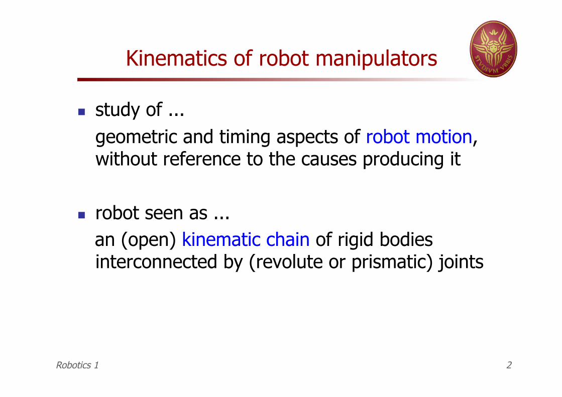
Kinematics of robot manipulators

  study of ... geometric and timing aspects of robot motion, without reference to the causes producing it

  robot seen as ... an (open) kinematic chain of rigid bodies

interconnected by (revolute or prismatic) joints

Robotics 1 2

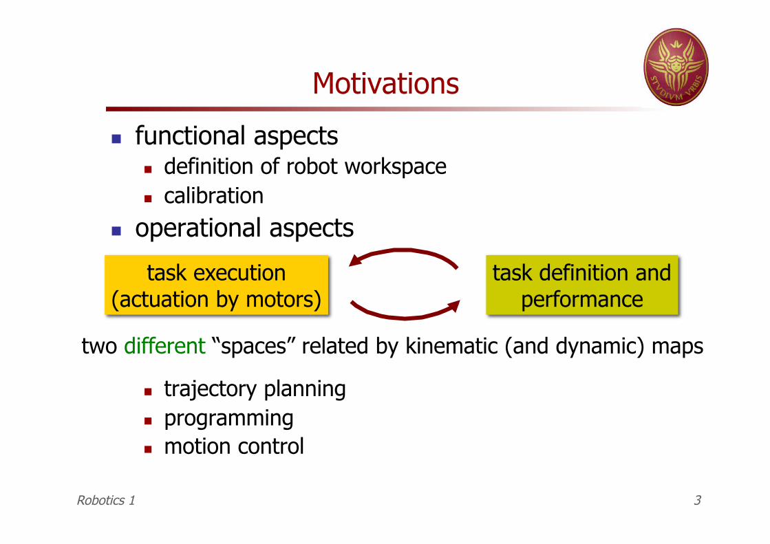
Motivations

  functional aspects   definition of robot workspace   calibration

  operational aspects

  trajectory planning   programming   motion control

task execution (actuation by motors)

task definition and performance

two different “spaces” related by kinematic (and dynamic) maps

Robotics 1 3

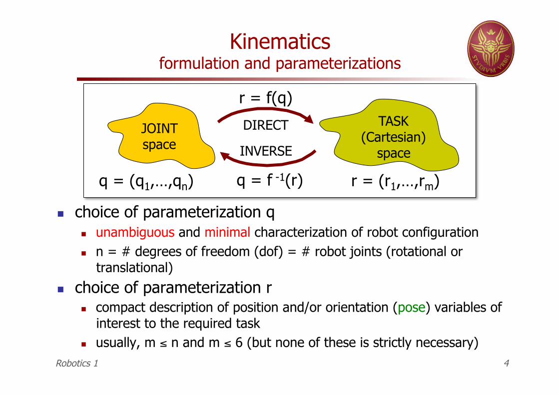
Kinematics formulation and parameterizations

  choice of parameterization q   unambiguous and minimal characterization of robot configuration   n = # degrees of freedom (dof) = # robot joints (rotational or

translational)

  choice of parameterization r   compact description of position and/or orientation (pose) variables of

interest to the required task   usually, m ≤ n and m ≤ 6 (but none of these is strictly necessary)

JOINT space

TASK (Cartesian)

space

q = (q1,…,qn) r = (r1,…,rm)

DIRECT

INVERSE

r = f(q)

q = f -1(r)

Robotics 1 4

Open kinematic chains

  m = 2   pointing in space   positioning in the plane

  m = 3   orientation in space   positioning and orientation in the plane

q1

q2

q3

q4

qn

r = (r1,…,rm)

e.g., it describes the pose of frame RFE

RFE

e.g., the relative angle between a link and the

following one

Robotics 1 5

  m = 5   positioning and pointing in space

  m = 6   positioning and orientation in

space (like for spot welding)   positioning of two points in space

(e.g., end-effector and elbow)

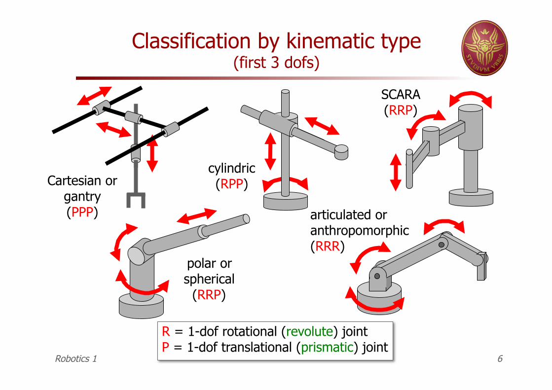
Classification by kinematic type (first 3 dofs)

Cartesian or gantry (PPP)

cylindric (RPP)

SCARA (RRP)

polar or spherical

(RRP)

articulated or anthropomorphic (RRR)

R = 1-dof rotational (revolute) joint P = 1-dof translational (prismatic) joint

Robotics 1 6

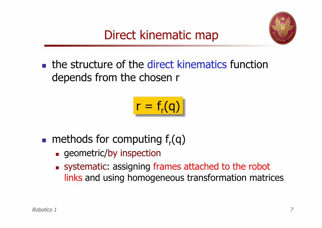
Direct kinematic map

  the structure of the direct kinematics function depends from the chosen r

  methods for computing fr(q)   geometric/by inspection   systematic: assigning frames attached to the robot

links and using homogeneous transformation matrices

r = fr(q)

Robotics 1 7

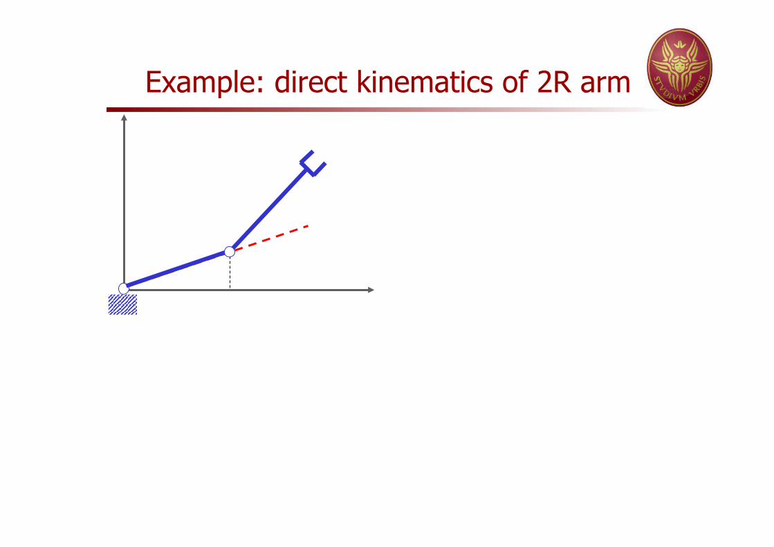
Example: direct kinematics of 2R arm

x

y

q1

q2

P • 

l1

l2

px

py φ q = q =

q1

q2

r = px py φ

n = 2

m = 3

px = l1 cos q1 + l2 cos(q1+q2)

py = l1 sin q1 + l2 sin(q1+q2)

φ = q1+ q2

for more general cases, we need a “method”! Robotics 1 8

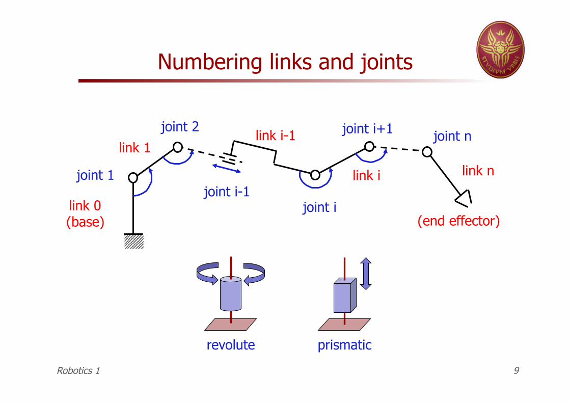
Numbering links and joints

joint 1

link 0 (base)

link 1

joint 2

joint i-1 joint i

joint n joint i+1 link i-1

link i link n

(end effector)

Robotics 1 9

revolute prismatic

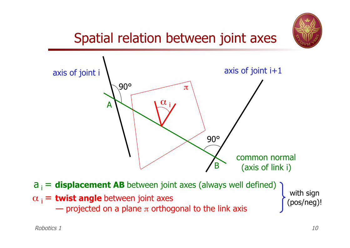
Spatial relation between joint axes

axis of joint i axis of joint i+1

common normal (axis of link i)

90°

90°

A

B

a i = displacement AB between joint axes (always well defined)

α i

π

α i = twist angle between joint axes — projected on a plane π orthogonal to the link axis

with sign (pos/neg)!

Robotics 1 10

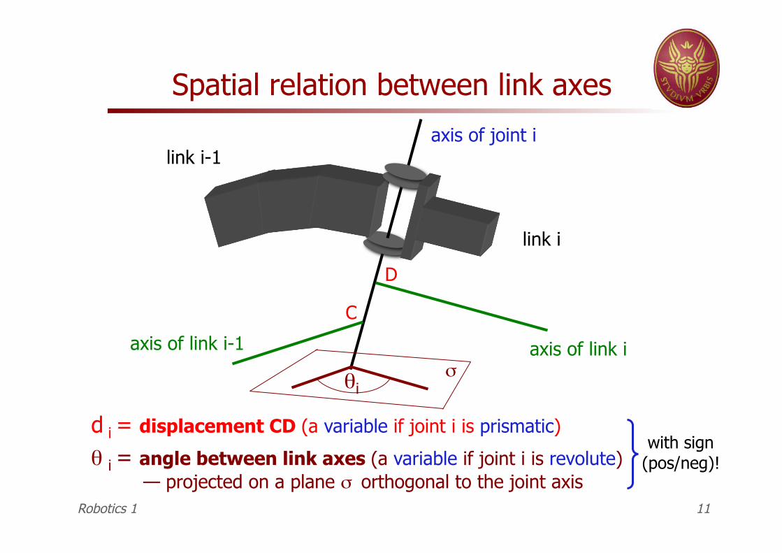
Spatial relation between link axes

link i-1

link i

axis of joint i

axis of link i axis of link i-1

C

D

d i = displacement CD (a variable if joint i is prismatic)

θ i = angle between link axes (a variable if joint i is revolute) — projected on a plane σ orthogonal to the joint axis

θi σ

with sign (pos/neg)!

Robotics 1 11

αi

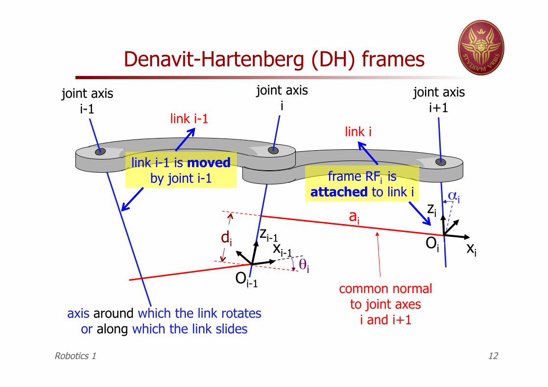
Denavit-Hartenberg (DH) frames

joint axis i-1

joint axis i

joint axis i+1

link i-1 link i

xi-1

Oi-1

xi

zi

Oi

ai

θi

zi-1 di

common normal to joint axes

i and i+1 axis around which the link rotates or along which the link slides

Robotics 1 12

frame RFi is attached to link i

link i-1 is moved by joint i-1

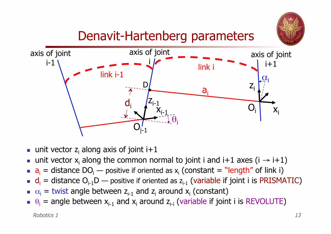
Denavit-Hartenberg parameters

  unit vector zi along axis of joint i+1   unit vector xi along the common normal to joint i and i+1 axes (i → i+1)   ai = distance DOi — positive if oriented as xi (constant = “length” of link i)   di = distance Oi-1D — positive if oriented as zi-1 (variable if joint i is PRISMATIC)   αi = twist angle between zi-1 and zi around xi (constant)   θi = angle between xi-1 and xi around zi-i (variable if joint i is REVOLUTE)

axis of joint i-1

axis of joint i

axis of joint i+1

link i-1 link i

xi-1

Oi-1

xi

zi

Oi

ai

θi

αi

zi-1 di

D • 

Robotics 1 13

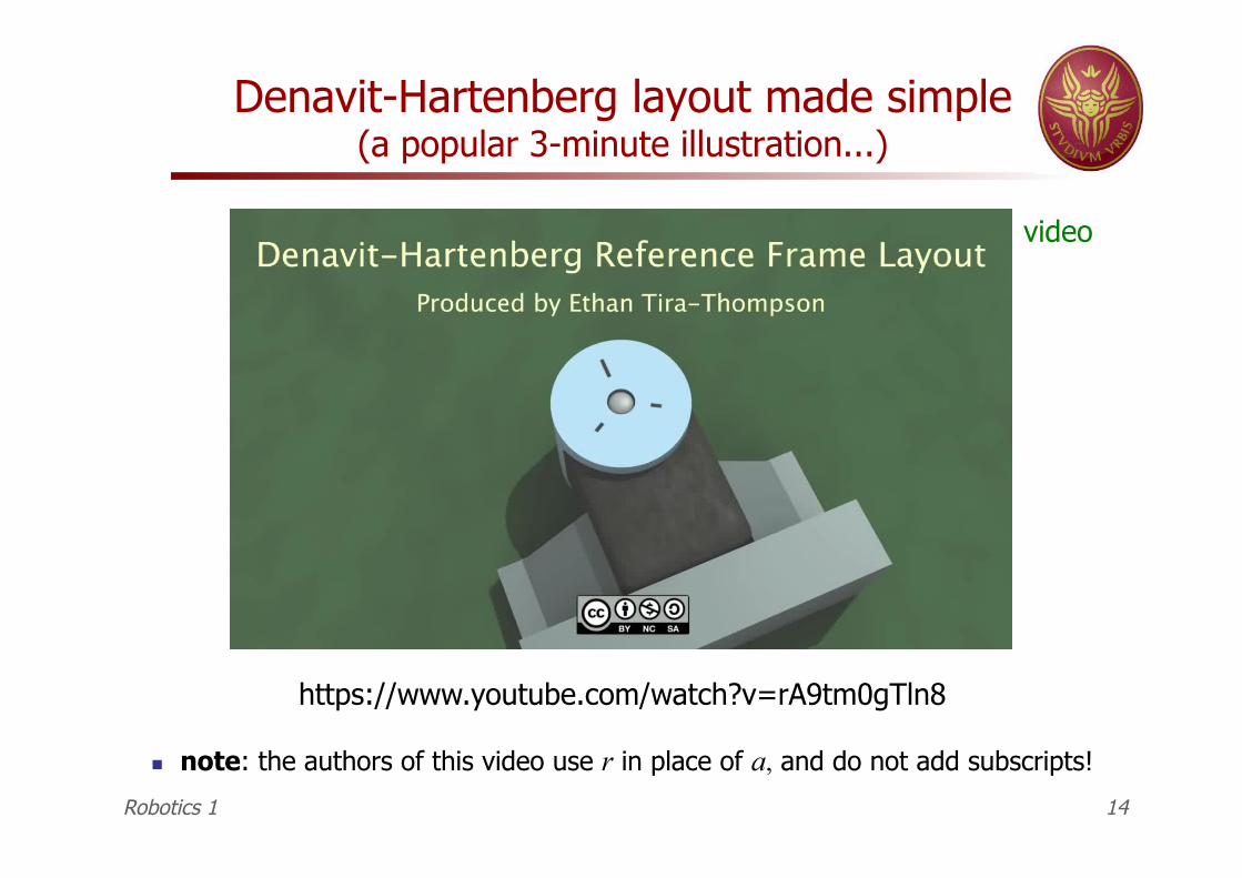
Denavit-Hartenberg layout made simple (a popular 3-minute illustration...)

  note: the authors of this video use r in place of a, and do not add subscripts! Robotics 1 14

video

https://www.youtube.com/watch?v=rA9tm0gTln8

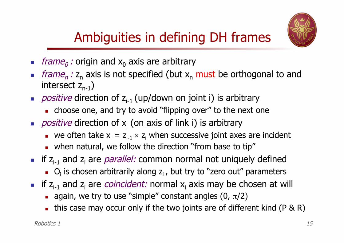
Ambiguities in defining DH frames

  frame0 : origin and x0 axis are arbitrary   framen : zn axis is not specified (but xn must be orthogonal to and

intersect zn-1)   positive direction of zi-1 (up/down on joint i) is arbitrary

  choose one, and try to avoid “flipping over” to the next one

  positive direction of xi (on axis of link i) is arbitrary   we often take xi = zi-1 × zi when successive joint axes are incident   when natural, we follow the direction “from base to tip”

  if zi-1 and zi are parallel: common normal not uniquely defined   Oi is chosen arbitrarily along zi , but try to “zero out” parameters

  if zi-1 and zi are coincident: normal xi axis may be chosen at will   again, we try to use “simple” constant angles (0, π/2)   this case may occur only if the two joints are of different kind (P & R)

Robotics 1 15

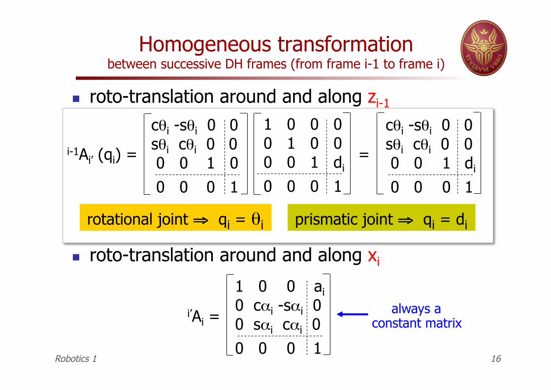
Homogeneous transformation between successive DH frames (from frame i-1 to frame i)

  roto-translation around and along zi-1

  roto-translation around and along xi

cθi -sθi 0 0 sθi cθi 0 0 0 0 1 0

0 0 0 1

1 0 0 0 0 1 0 0 0 0 1 di

0 0 0 1

cθi -sθi 0 0 sθi cθi 0 0 0 0 1 di

0 0 0 1

i-1Ai’ (qi) = =

rotational joint ⇒ qi = θi prismatic joint ⇒ qi = di

1 0 0 ai 0 cαi -sαi 0 0 sαi cαi 0

0 0 0 1

i’Ai = always a

constant matrix

Robotics 1 16

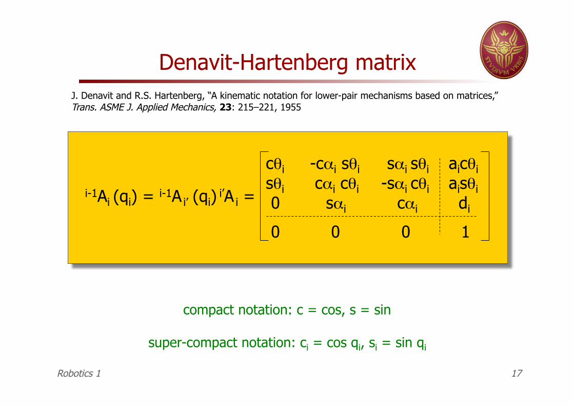
Denavit-Hartenberg matrix

cθi -cαi sθi sαi sθi aicθi sθi cαi cθi -sαi cθi aisθi 0 sαi cαi di

0 0 0 1

i-1Ai (qi) = i-1A i’ (qi) i’A i =

compact notation: c = cos, s = sin

super-compact notation: ci = cos qi, si = sin qi

Robotics 1 17

J. Denavit and R.S. Hartenberg, “A kinematic notation for lower-pair mechanisms based on matrices,” Trans. ASME J. Applied Mechanics, 23: 215–221, 1955

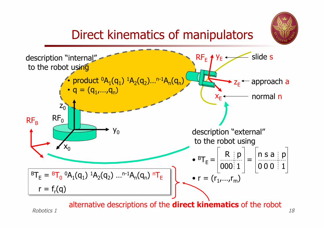
Direct kinematics of manipulators

xE

yE

zE approach a

slide s

normal n

description “internal” to the robot using

•  product 0A1(q1) 1A2(q2)…n-1An(qn) •  q = (q1,…,qn)

description “external” to the robot using

•  BTE = =

•  r = (r1,…,rm)

R p

000 1

n s a p

0 0 0 1 BTE = BT0 0A1(q1) 1A2(q2) …n-1An(qn) nTE

r = fr(q)

alternative descriptions of the direct kinematics of the robot

RFB

Robotics 1 18

x0

y0

z0

RF0

RFE

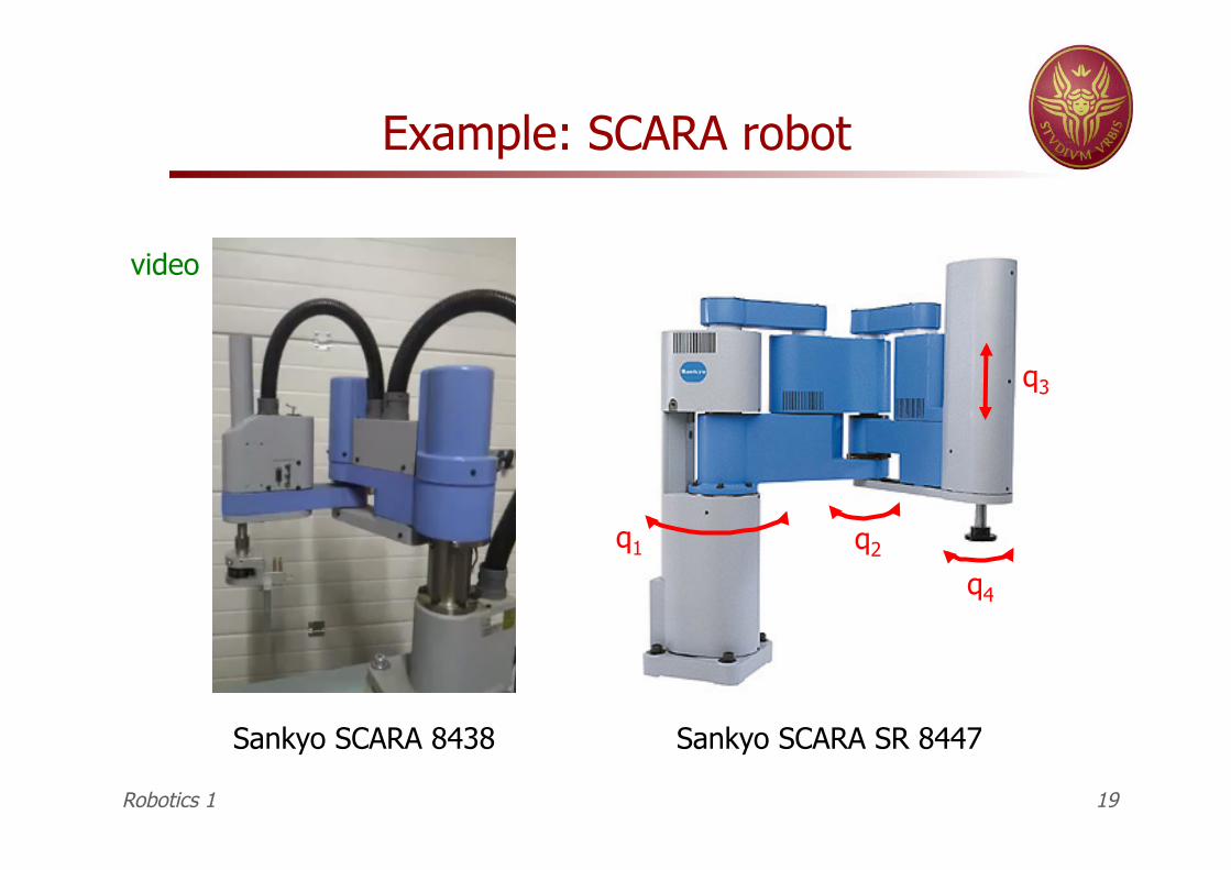
Example: SCARA robot

q1 q2

q3

q4

Robotics 1 19

Sankyo SCARA 8438

video

Sankyo SCARA SR 8447

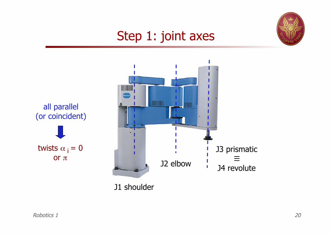
J1 shoulder

J2 elbow

J3 prismatic ≡

J4 revolute

Step 1: joint axes

all parallel (or coincident)

twists α i = 0 or π

Robotics 1 20

a1

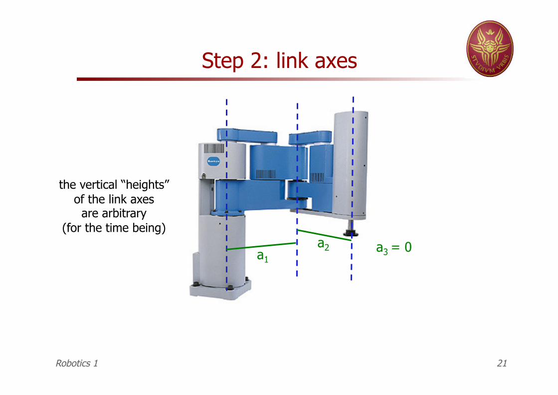
Step 2: link axes

a2 a3 = 0

the vertical “heights” of the link axes

are arbitrary (for the time being)

Robotics 1 21

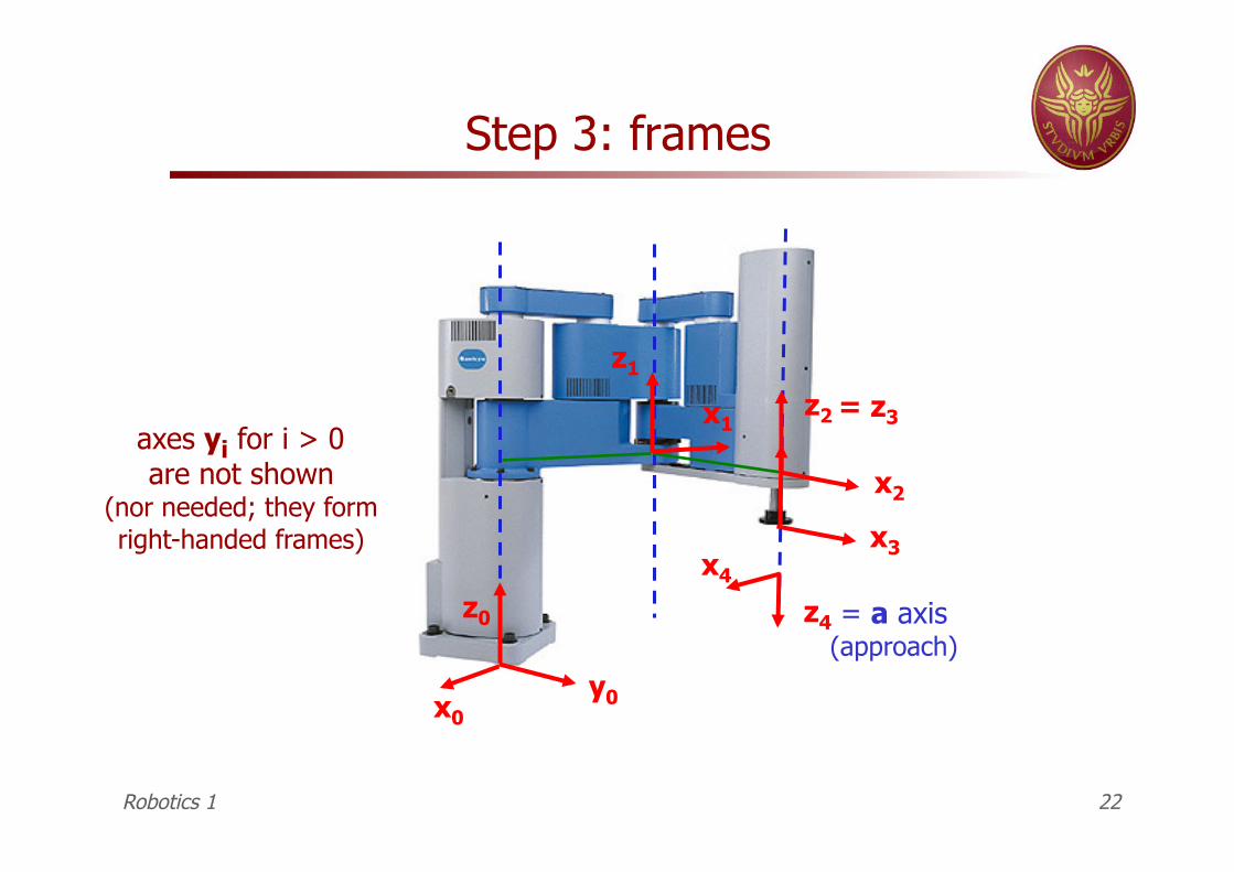
Step 3: frames

= a axis (approach)

z0

x0 y0

= z3

x3

z4 x4

axes yi for i > 0 are not shown

(nor needed; they form right-handed frames)

Robotics 1 22

z2

x2

z1

x1

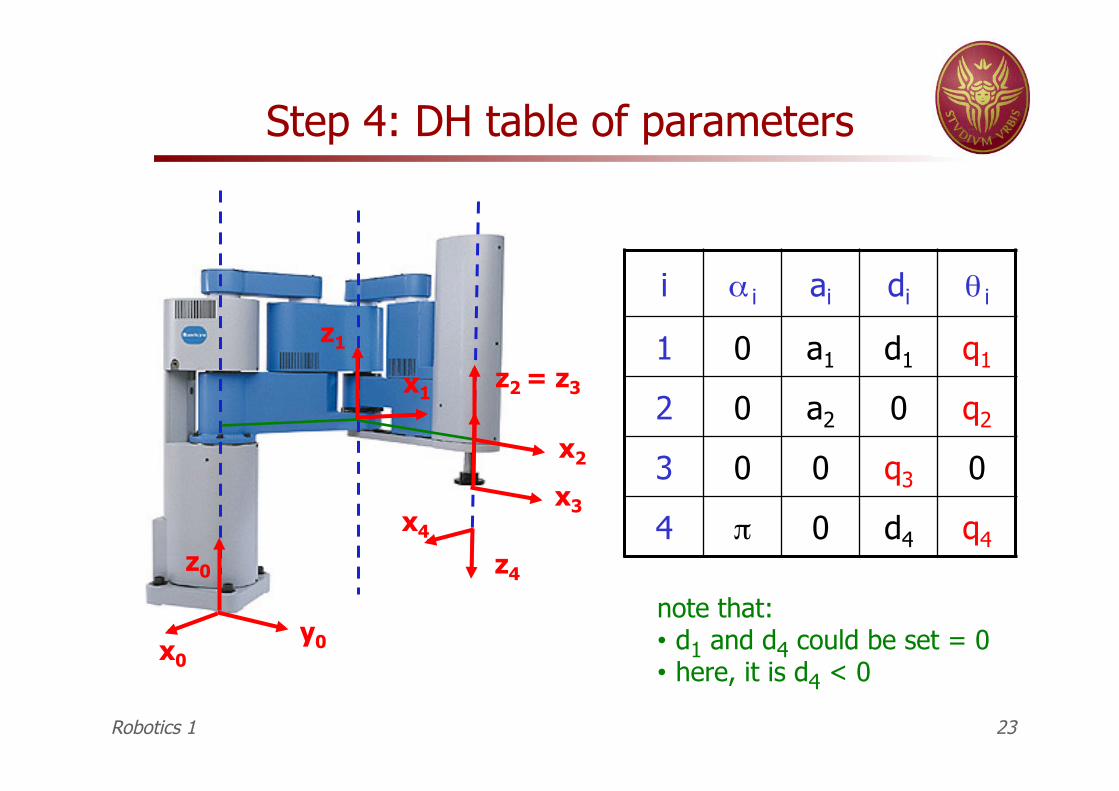
Step 4: DH table of parameters

i α i ai di θ i

1 0 a1 d1 q1

2 0 a2 0 q2

3 0 0 q3 0

4 π 0 d4 q4

note that: •  d1 and d4 could be set = 0 •  here, it is d4 < 0

Robotics 1 23

z0

x0 y0

= z3

x3

z4 x4

z1

x1 z2

x2

Step 5: transformation matrices

cθ4 sθ4 0 0 sθ4 -cθ4 0 0 0 0 -1 d4 0 0 0 1

1 0 0 0 0 1 0 0 0 0 1 d3 0 0 0 1

cθ2 - sθ2 0 a2cθ2 sθ2 cθ2 0 a2sθ2 0 0 1 0 0 0 0 1

cθ1 - sθ1 0 a1cθ1 sθ1 cθ1 0 a1sθ1 0 0 1 d1 0 0 0 1

3A4(q4) =

2A3(q3) = 1A2(q2) =

0A1(q1) =

q = (q1, q2, q3, q4)

= (θ1, θ2, d3, θ4)

Robotics 1 24

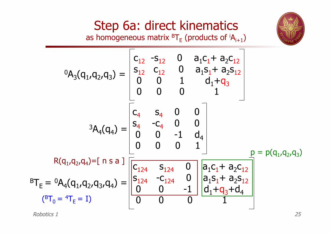
Step 6a: direct kinematics as homogeneous matrix BTE (products of iAi+1)

c4 s4 0 0 s4 -c4 0 0 0 0 -1 d4 0 0 0 1

c12 -s12 0 a1c1+ a2c12 s12 c12 0 a1s1+ a2s12 0 0 1 d1+q3 0 0 0 1

3A4(q4) =

0A3(q1,q2,q3) =

c124 s124 0 a1c1+ a2c12 s124 -c124 0 a1s1+ a2s12 0 0 -1 d1+q3+d4 0 0 0 1

BTE = 0A4(q1,q2,q3,q4) =

p = p(q1,q2,q3) R(q1,q2,q4)=[ n s a ]

Robotics 1 25

(BT0 = 4TE = I)

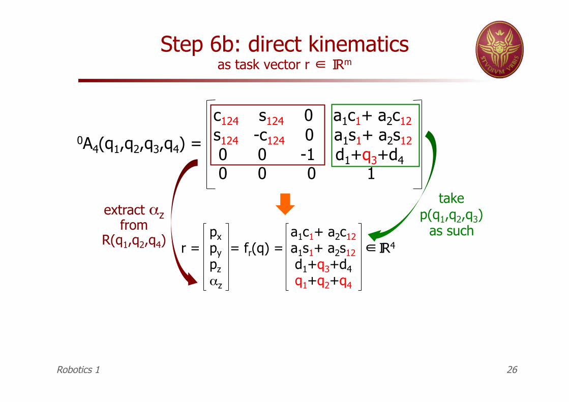
Step 6b: direct kinematics as task vector r ∈ Rm

take p(q1,q2,q3)

as such

c124 s124 0 a1c1+ a2c12 s124 -c124 0 a1s1+ a2s12 0 0 -1 d1+q3+d4 0 0 0 1

0A4(q1,q2,q3,q4) =

extract αz from

R(q1,q2,q4)

Robotics 1 26

px a1c1+ a2c12 r = py = fr(q) = a1s1+ a2s12 ∈ R4

pz d1+q3+d4 αz q1+q2+q4

I

I

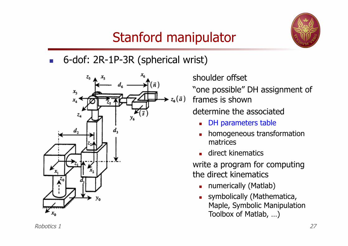
Stanford manipulator

  6-dof: 2R-1P-3R (spherical wrist)

  shoulder offset   “one possible” DH assignment of

frames is shown   determine the associated

  DH parameters table   homogeneous transformation

matrices   direct kinematics

  write a program for computing the direct kinematics

  numerically (Matlab)   symbolically (Mathematica,

Maple, Symbolic Manipulation Toolbox of Matlab, …)

Robotics 1 27

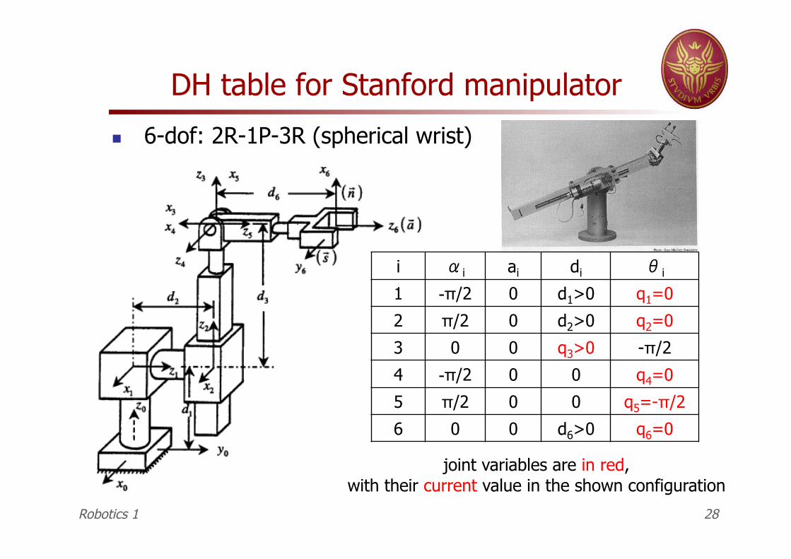
DH table for Stanford manipulator

  6-dof: 2R-1P-3R (spherical wrist)

Robotics 1 28

i αi ai di θi

1 -π/2 0 d1>0 q1=0

2 π/2 0 d2>0 q2=0

3 0 0 q3>0 -π/2

4 -π/2 0 0 q4=0

5 π/2 0 0 q5=-π/2

6 0 0 d6>0 q6=0

joint variables are in red, with their current value in the shown configuration

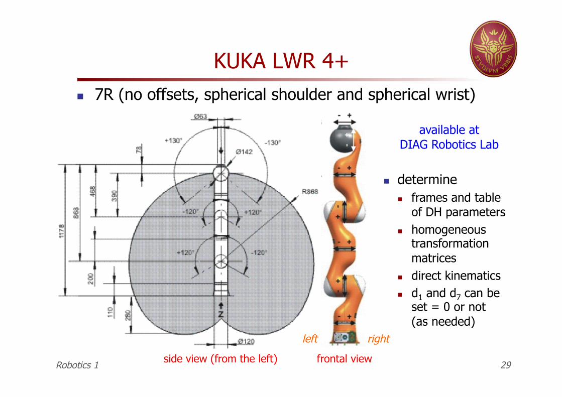
KUKA LWR 4+   7R (no offsets, spherical shoulder and spherical wrist)

  determine   frames and table

of DH parameters   homogeneous

transformation matrices

  direct kinematics   d1 and d7 can be

set = 0 or not (as needed)

available at DIAG Robotics Lab

Robotics 1 29 frontal view side view (from the left)

left right

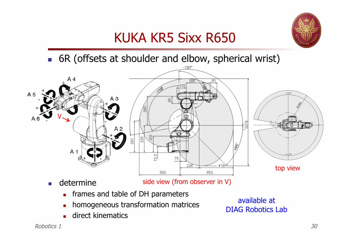
KUKA KR5 Sixx R650   6R (offsets at shoulder and elbow, spherical wrist)

  determine   frames and table of DH parameters   homogeneous transformation matrices   direct kinematics

available at DIAG Robotics Lab

Robotics 1 30

top view

side view (from observer in V)

V

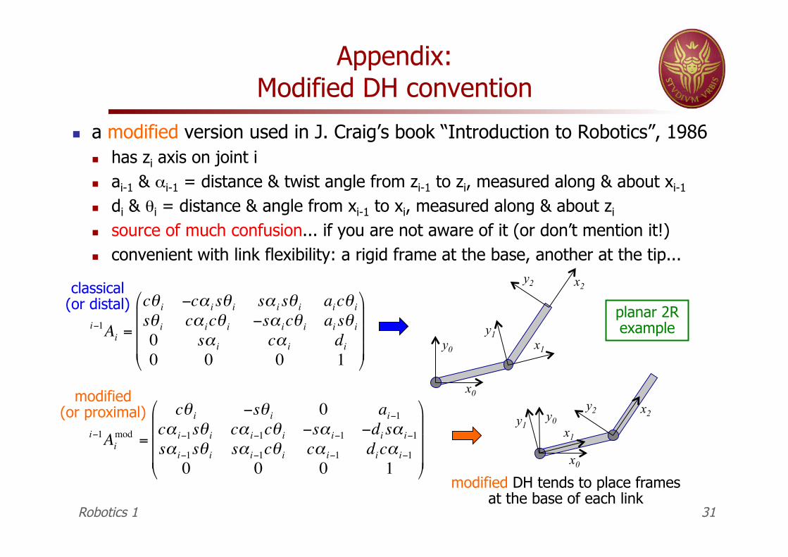
Appendix: Modified DH convention

  a modified version used in J. Craig’s book “Introduction to Robotics”, 1986   has zi axis on joint i   ai-1 & αi-1 = distance & twist angle from zi-1 to zi, measured along & about xi-1

  di & θi = distance & angle from xi-1 to xi, measured along & about zi   source of much confusion... if you are not aware of it (or don’t mention it!)   convenient with link flexibility: a rigid frame at the base, another at the tip...

Robotics 1 31

€

i−1Aimod =

cθ i −sθ i 0 ai−1cα i−1sθ i cα i−1cθ i −sα i−1 −di sα i−1sα i−1sθ i sα i−1cθ i cα i−1 dicα i−10 0 0 1

⎛

⎝

⎜ ⎜ ⎜

⎞

⎠

⎟ ⎟ ⎟

€

i−1Ai =

cθ i −cα i sθ i sα i sθ i aicθ isθ i cα icθ i −sα icθ i ai sθ i0 sα i cα i di0 0 0 1

⎛

⎝

⎜ ⎜ ⎜

⎞

⎠

⎟ ⎟ ⎟

modified DH tends to place frames at the base of each link

x0

y0 x1

y1

x2 y2

x0

y0 x1

y1

x2 y2

planar 2R example

classical (or distal)

modified (or proximal)