RF Systems I - cas.web.cern.ch delay of 𝜏 becomes ... So I and Q are the Cartesian coordinates in...

RF Systems I Erk Jensen, CERN BE-RF

Introduction to Accelerator Physics, Prague, Czech Republic, 31 Aug – 12 Sept 2014

Definitions & basic concepts dB

t-domain vs. ω-domain

phasors

8th Sept, 2014 CAS Prague - EJ: RF Systems I 2

Decibel (dB)

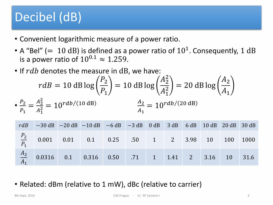
• Convenient logarithmic measure of a power ratio.

• A “Bel” (= 10 dB) is defined as a power ratio of 101. Consequently, 1 dB is a power ratio of 100.1 ≈ 1.259.

• If 𝑟𝑑𝑏 denotes the measure in dB, we have:

𝑟𝑑𝐵 = 10 dB log𝑃2

𝑃1= 10 dB log

𝐴22

𝐴12 = 20 dB log

𝐴2

𝐴1

•𝑃2

𝑃1=

𝐴22

𝐴12 = 10𝑟𝑑𝑏 10 dB

𝐴2

𝐴1= 10𝑟𝑑𝑏 20 dB

• Related: dBm (relative to 1 mW), dBc (relative to carrier) 8th Sept, 2014 CAS Prague - EJ: RF Systems I 3

𝑟𝑑𝐵 −30 dB −20 dB −10 dB −6 dB −3 dB 0 dB 3 dB 6 dB 10 dB 20 dB 30 dB

𝑃2

𝑃1 0.001 0.01 0.1 0.25 .50 1 2 3.98 10 100 1000

𝐴2

𝐴1 0.0316 0.1 0.316 0.50 .71 1 1.41 2 3.16 10 31.6

Time domain – frequency domain (1)

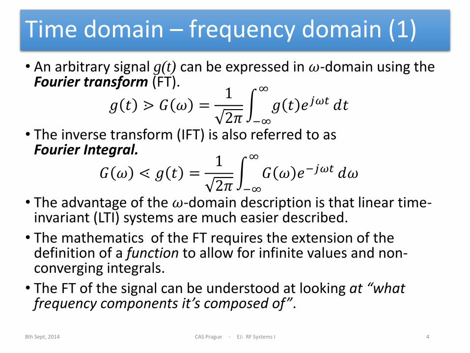
• An arbitrary signal g(t) can be expressed in 𝜔-domain using the Fourier transform (FT).

𝑔 𝑡 ⋗ 𝐺 𝜔 =1

2𝜋 𝑔 𝑡 ⅇⅉ𝜔𝑡

∞

−∞

𝑑𝑡

• The inverse transform (IFT) is also referred to as Fourier Integral.

𝐺 𝜔 ⋖ 𝑔 𝑡 =1

2𝜋 𝐺 𝜔 ⅇ−ⅉ𝜔𝑡

∞

−∞

𝑑𝜔

• The advantage of the 𝜔-domain description is that linear time-invariant (LTI) systems are much easier described.

• The mathematics of the FT requires the extension of the definition of a function to allow for infinite values and non-converging integrals.

• The FT of the signal can be understood at looking at “what frequency components it’s composed of”.


Time domain – frequency domain (2)

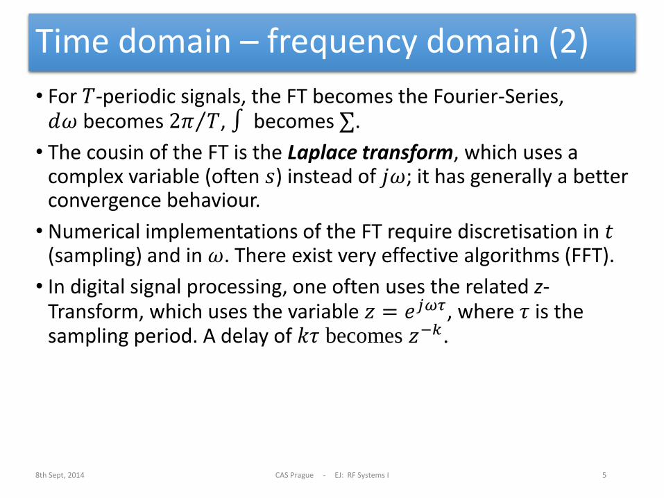
• For 𝑇-periodic signals, the FT becomes the Fourier-Series, 𝑑𝜔 becomes 2𝜋 𝑇 , ∫ becomes ∑.

• The cousin of the FT is the Laplace transform, which uses a complex variable (often 𝑠) instead of ⅉ𝜔; it has generally a better convergence behaviour.

• Numerical implementations of the FT require discretisation in 𝑡 (sampling) and in 𝜔. There exist very effective algorithms (FFT).

• In digital signal processing, one often uses the related z-Transform, which uses the variable 𝑧 = ⅇⅉ𝜔𝜏, where 𝜏 is the sampling period. A delay of 𝑘𝜏 becomes 𝑧−𝑘.


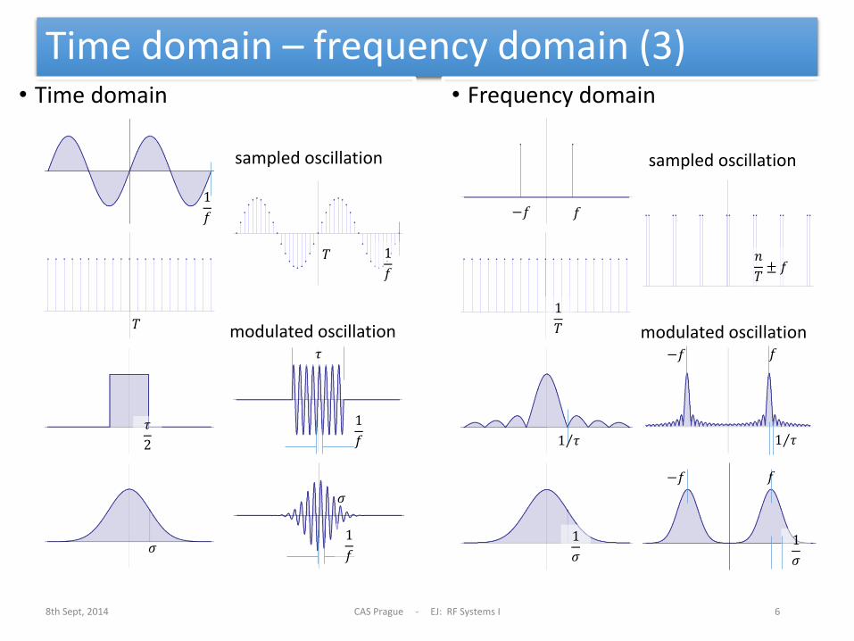
Time domain – frequency domain (3) • Time domain • Frequency domain


𝑓 −𝑓

𝜏

2 1 𝜏

𝜎 1

𝜎

𝑇 1

𝑇

1

𝑓

𝑛

𝑇± 𝑓

1

𝑓

𝑇

1

𝜎

𝑓 −𝑓

𝜎

1

𝑓

sampled oscillation sampled oscillation

modulated oscillation modulated oscillation

1

𝑓

𝜏 −𝑓

1 𝜏

𝑓

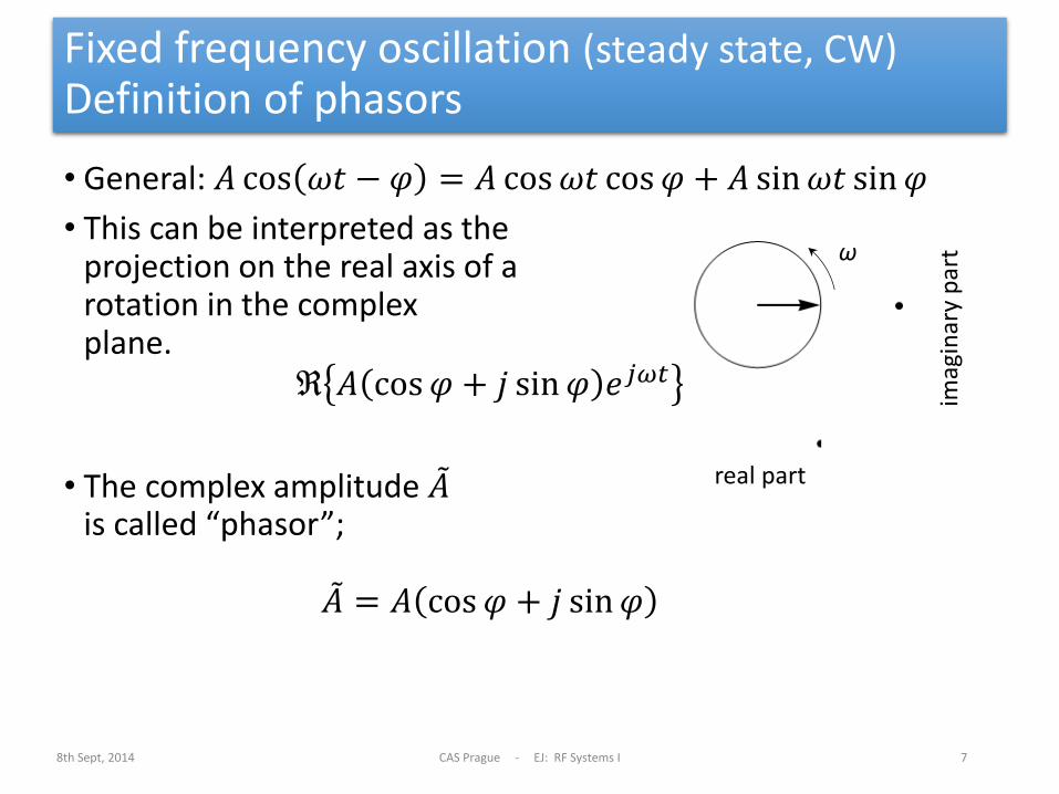
Fixed frequency oscillation (steady state, CW) Definition of phasors

• General: 𝐴 cos 𝜔𝑡 − 𝜑 = 𝐴 cos 𝜔𝑡 cos 𝜑 + 𝐴 sin 𝜔𝑡 sin 𝜑

• This can be interpreted as the projection on the real axis of a rotation in the complex plane.

ℜ 𝐴 cos 𝜑 + ⅉ sin 𝜑 ⅇⅉ𝜔𝑡

• The complex amplitude 𝐴 is called “phasor”;

𝐴 = 𝐴 cos 𝜑 + ⅉ sin 𝜑


real part

imag

inar

y p

art ω

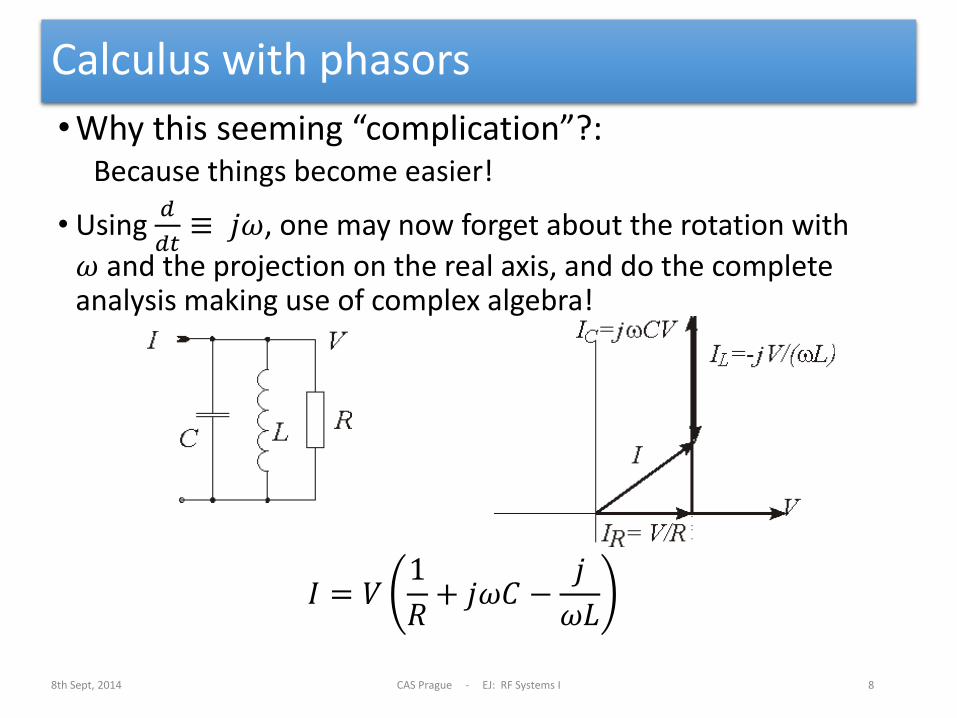
Calculus with phasors

•Why this seeming “complication”?: Because things become easier!

• Using 𝑑

𝑑𝑡≡ ⅉ𝜔, one may now forget about the rotation with

𝜔 and the projection on the real axis, and do the complete analysis making use of complex algebra!

𝐼 = 𝑉1

𝑅+ ⅉ𝜔𝐶 −

ⅉ

𝜔𝐿


Example:

Slowly varying amplitudes

• For band-limited signals, one may conveniently use “slowly varying” phasors and a fixed frequency RF oscillation.

• So-called in-phase (I) and quadrature (Q) “baseband envelopes” of a modulated RF carrier are the real and imaginary part of a slowly varying phasor.


On Modulation AM

PM

I-Q


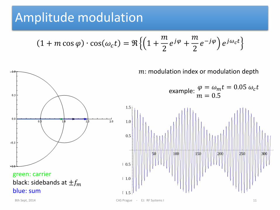
Amplitude modulation

1 + 𝑚 cos 𝜑 ∙ cos 𝜔𝑐𝑡 = ℜ 1 +𝑚

2ⅇⅉ𝜑 +

𝑚

2ⅇ−ⅉ𝜑 ⅇⅉ𝜔𝑐𝑡


50 100 150 200 250 300

1.5

1.0

0.5

0.5

1.0

1.5

green: carrier black: sidebands at ±𝑓𝑚 blue: sum

example: 𝜑 = 𝜔𝑚𝑡 = 0.05 𝜔𝑐𝑡𝑚 = 0.5

𝑚: modulation index or modulation depth

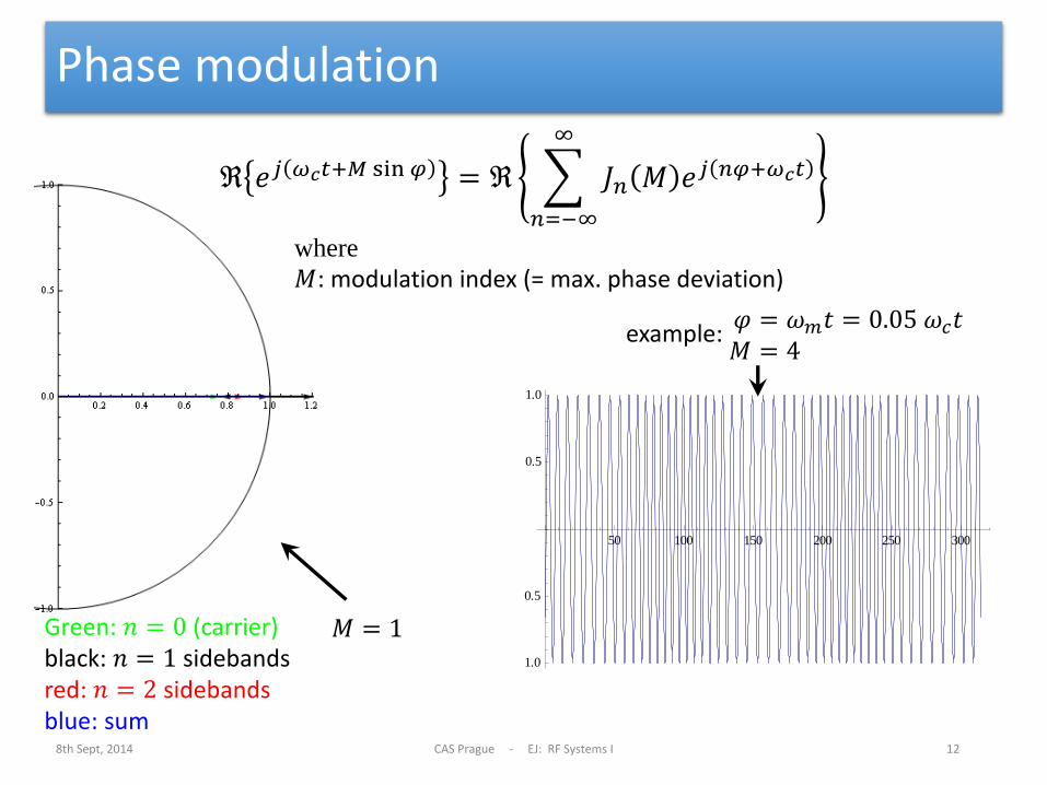
Phase modulation

ℜ ⅇⅉ 𝜔𝑐𝑡+𝑀 sin 𝜑 = ℜ 𝐽𝑛 𝑀 ⅇⅉ 𝑛𝜑+𝜔𝑐𝑡

∞

𝑛=−∞


50 100 150 200 250 300

1.0

0.5

0.5

1.0

Green: 𝑛 = 0 (carrier) black: 𝑛 = 1 sidebands red: 𝑛 = 2 sidebands blue: sum

where

𝑀: modulation index (= max. phase deviation)

example: 𝜑 = 𝜔𝑚𝑡 = 0.05 𝜔𝑐𝑡𝑀 = 4

𝑀 = 1

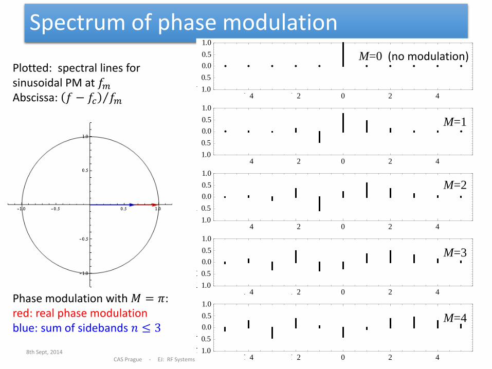
Spectrum of phase modulation

8th Sept, 2014 CAS Prague - EJ: RF Systems I

13

4 2 0 2 41.0

0.5

0.0

0.5

1.0

4 2 0 2 41.0

0.5

0.0

0.5

1.0

4 2 0 2 41.0

0.5

0.0

0.5

1.0

4 2 0 2 41.0

0.5

0.0

0.5

1.0

4 2 0 2 41.0

0.5

0.0

0.5

1.0Phase modulation with 𝑀 = 𝜋: red: real phase modulation blue: sum of sidebands 𝑛 ≤ 3

M=1

M=4

M=3

M=2

Plotted: spectral lines for sinusoidal PM at 𝑓𝑚 Abscissa: 𝑓 − 𝑓𝑐 𝑓𝑚

M=0 (no modulation)

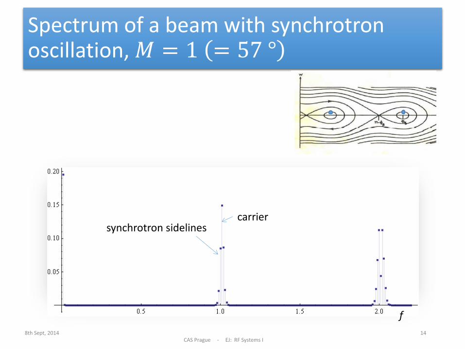
Spectrum of a beam with synchrotron oscillation, 𝑀 = 1 = 57 °


14

carrier synchrotron sidelines

f

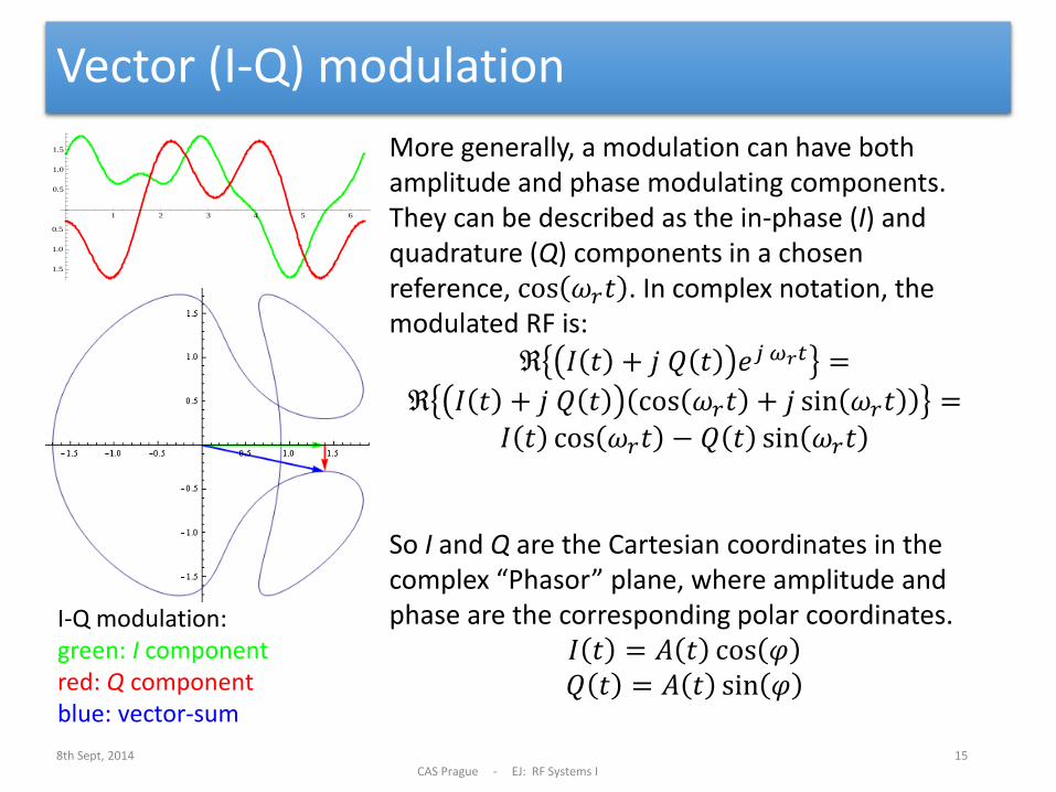
Vector (I-Q) modulation


15

More generally, a modulation can have both amplitude and phase modulating components. They can be described as the in-phase (I) and quadrature (Q) components in a chosen reference, cos 𝜔𝑟𝑡 . In complex notation, the modulated RF is:

ℜ 𝐼 𝑡 + ⅉ 𝑄 𝑡 ⅇⅉ 𝜔𝑟𝑡 =

ℜ 𝐼 𝑡 + ⅉ 𝑄 𝑡 cos 𝜔𝑟𝑡 + ⅉ sin 𝜔𝑟𝑡 =

𝐼 𝑡 cos 𝜔𝑟𝑡 − 𝑄 𝑡 sin 𝜔𝑟𝑡

So I and Q are the Cartesian coordinates in the complex “Phasor” plane, where amplitude and phase are the corresponding polar coordinates.

𝐼 𝑡 = 𝐴 𝑡 cos 𝜑 𝑄 𝑡 = 𝐴 𝑡 sin 𝜑

I-Q modulation: green: I component red: Q component blue: vector-sum

1 2 3 4 5 6

1.5

1.0

0.5

0.5

1.0

1.5

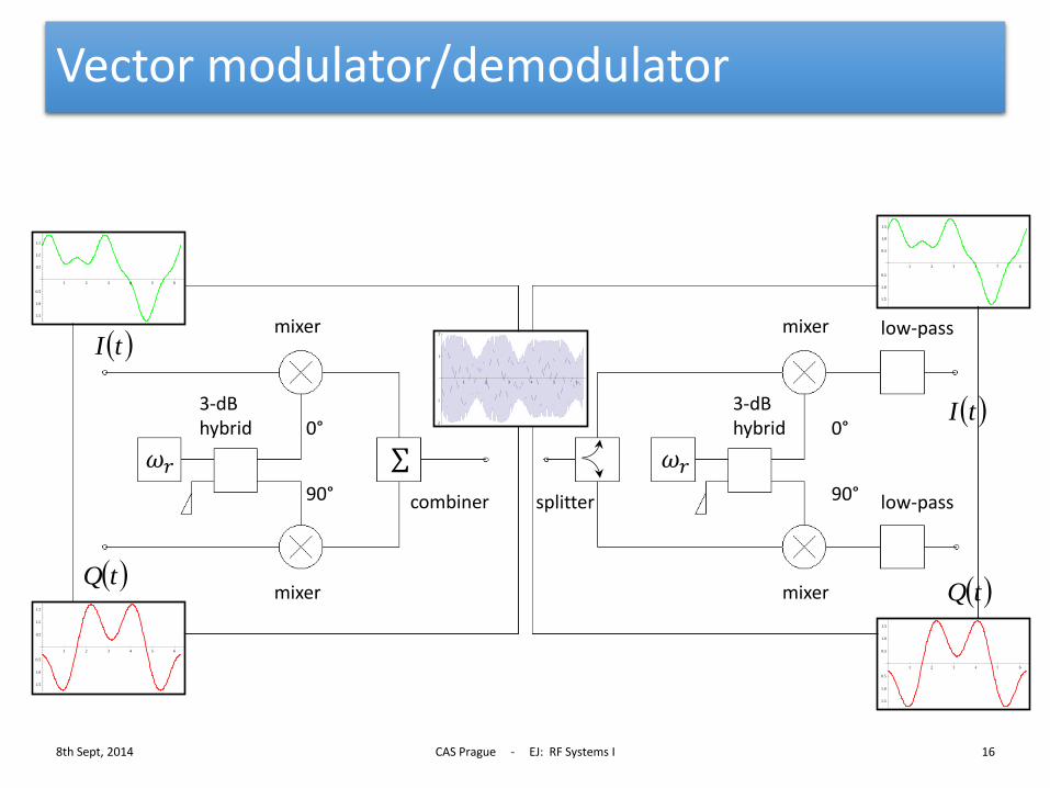
Vector modulator/demodulator


mixer

0°

90° combiner splitter

3-dB hybrid

low-pass

low-pass

tI

tI

tQ tQ

1 2 3 4 5 6

1.5

1.0

0.5

0.5

1.0

1.5

1 2 3 4 5 6

1.5

1.0

0.5

0.5

1.0

1.5

1 2 3 4 5 6

1.5

1.0

0.5

0.5

1.0

1.5

1 2 3 4 5 6

1.5

1.0

0.5

0.5

1.0

1.5

1 2 3 4 5 6

2

1

1

2

3-dB hybrid 0°

90°

𝜔𝑟 𝜔𝑟 ∑

mixer

mixer

mixer

Digital Signal Processing Just some basics


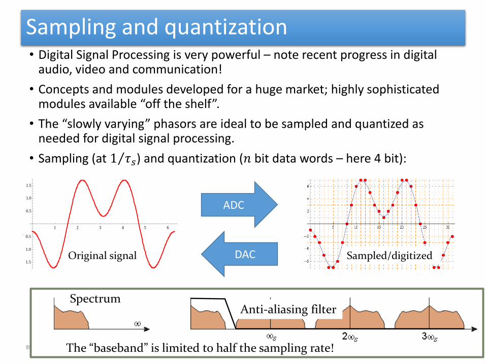
Sampling and quantization • Digital Signal Processing is very powerful – note recent progress in digital

audio, video and communication!

• Concepts and modules developed for a huge market; highly sophisticated modules available “off the shelf”.

• The “slowly varying” phasors are ideal to be sampled and quantized as needed for digital signal processing.

• Sampling (at 1 𝜏𝑠 ) and quantization (𝑛 bit data words – here 4 bit):


1 2 3 4 5 6

1.5

1.0

0.5

0.5

1.0

1.5

The “baseband” is limited to half the sampling rate!

ADC

DAC Original signal Sampled/digitized

Anti-aliasing filter Spectrum

The “baseband” is limited to half the sampling rate!

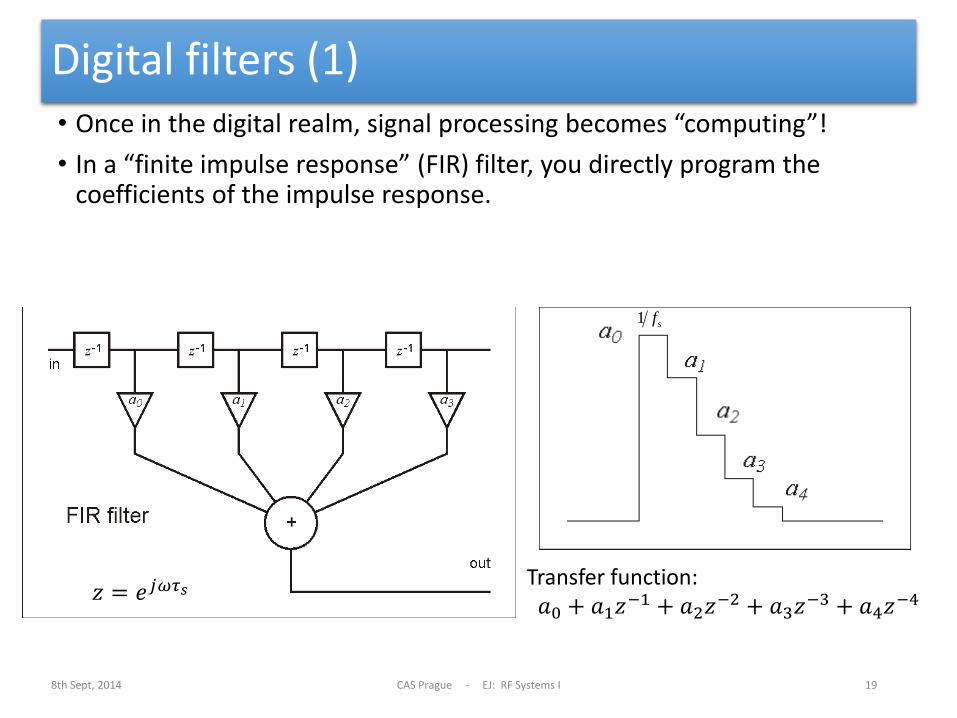
Digital filters (1) • Once in the digital realm, signal processing becomes “computing”!

• In a “finite impulse response” (FIR) filter, you directly program the coefficients of the impulse response.


sf1

Transfer function: 𝑎0 + 𝑎1𝑧

−1 + 𝑎2𝑧−2 + 𝑎3𝑧−3 + 𝑎4𝑧−4

𝑧 = ⅇⅉ𝜔𝜏𝑠

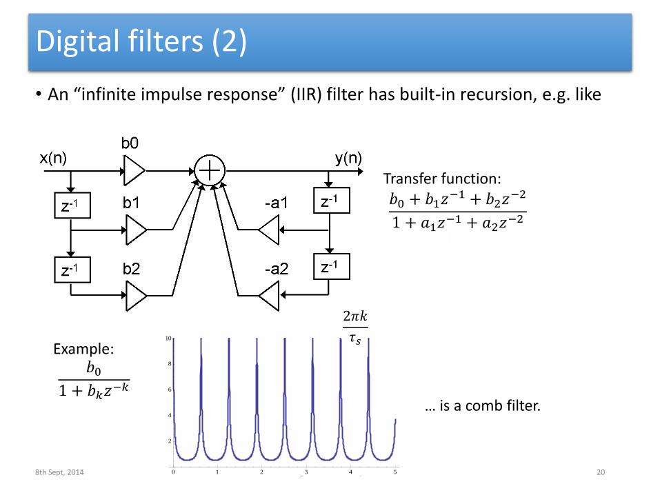
Digital filters (2)

• An “infinite impulse response” (IIR) filter has built-in recursion, e.g. like


Transfer function: 𝑏0 + 𝑏1𝑧−1 + 𝑏2𝑧−2

1 + 𝑎1𝑧−1 + 𝑎2𝑧−2

Example: 𝑏0

1 + 𝑏𝑘𝑧−𝑘

0 1 2 3 4 5

2

4

6

8

10

… is a comb filter.

2𝜋𝑘

𝜏𝑠

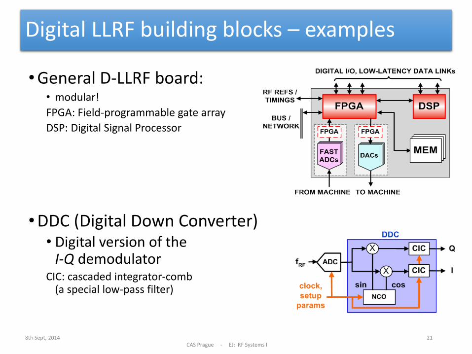
Digital LLRF building blocks – examples

•General D-LLRF board: • modular!

FPGA: Field-programmable gate array

DSP: Digital Signal Processor

•DDC (Digital Down Converter) • Digital version of the

I-Q demodulator CIC: cascaded integrator-comb

(a special low-pass filter)


21

RF system & control loops

e.g.: … for a synchrotron:

Cavity control loops

Beam control loops


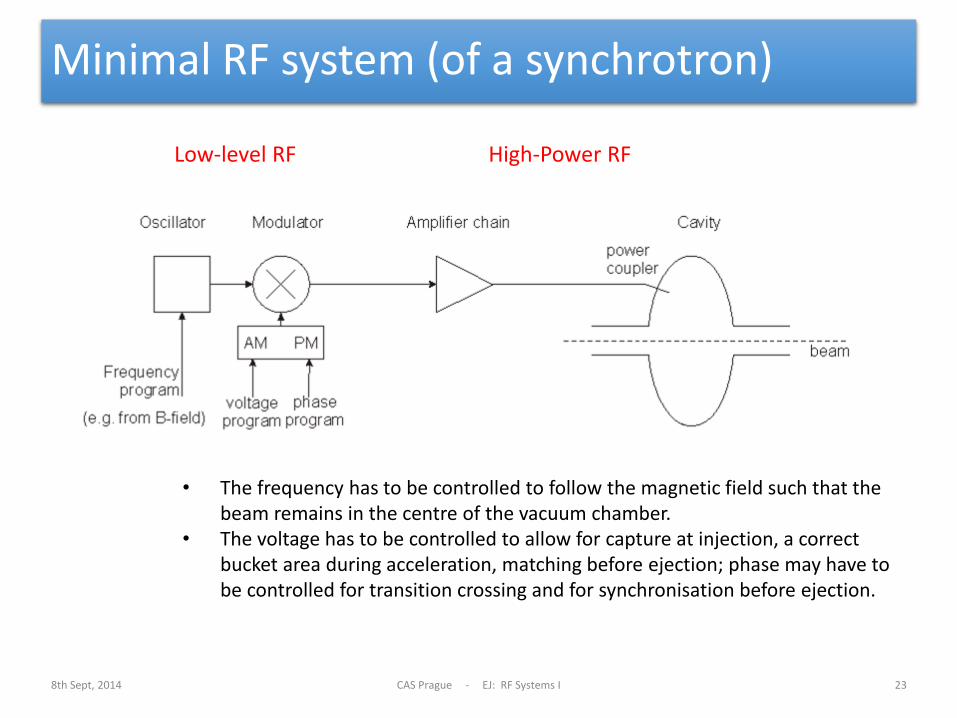
Minimal RF system (of a synchrotron)


• The frequency has to be controlled to follow the magnetic field such that the beam remains in the centre of the vacuum chamber.

• The voltage has to be controlled to allow for capture at injection, a correct bucket area during acceleration, matching before ejection; phase may have to be controlled for transition crossing and for synchronisation before ejection.

Low-level RF High-Power RF

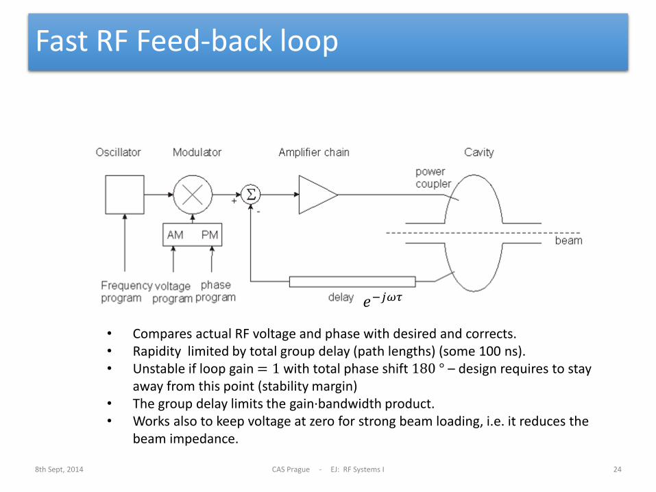
Fast RF Feed-back loop


• Compares actual RF voltage and phase with desired and corrects. • Rapidity limited by total group delay (path lengths) (some 100 ns). • Unstable if loop gain = 1 with total phase shift 180 ° – design requires to stay

away from this point (stability margin) • The group delay limits the gain·bandwidth product. • Works also to keep voltage at zero for strong beam loading, i.e. it reduces the

beam impedance.

ⅇ−ⅉ𝜔𝜏

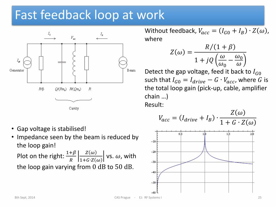
Fast feedback loop at work


Without feedback, 𝑉𝑎𝑐𝑐 = 𝐼𝐺0 + 𝐼𝐵 ∙ 𝑍 𝜔 , where

𝑍 𝜔 =𝑅 1 + 𝛽

1 + ⅉ𝑄𝜔𝜔0

−𝜔0𝜔

Detect the gap voltage, feed it back to 𝐼𝐺0 such that 𝐼𝐺0 = 𝐼𝑑𝑟𝑖𝑣𝑒 − 𝐺 ∙ 𝑉𝑎𝑐𝑐, where 𝐺 is the total loop gain (pick-up, cable, amplifier chain …) Result:

𝑉𝑎𝑐𝑐 = 𝐼𝑑𝑟𝑖𝑣𝑒 + 𝐼𝐵 ∙𝑍 𝜔

1 + 𝐺 ∙ 𝑍 𝜔

• Gap voltage is stabilised! • Impedance seen by the beam is reduced by

the loop gain!

Plot on the right: 1+𝛽

𝑅

𝑍 𝜔

1+𝐺∙𝑍 𝜔 vs. 𝜔, with

the loop gain varying from 0 dB to 50 dB.

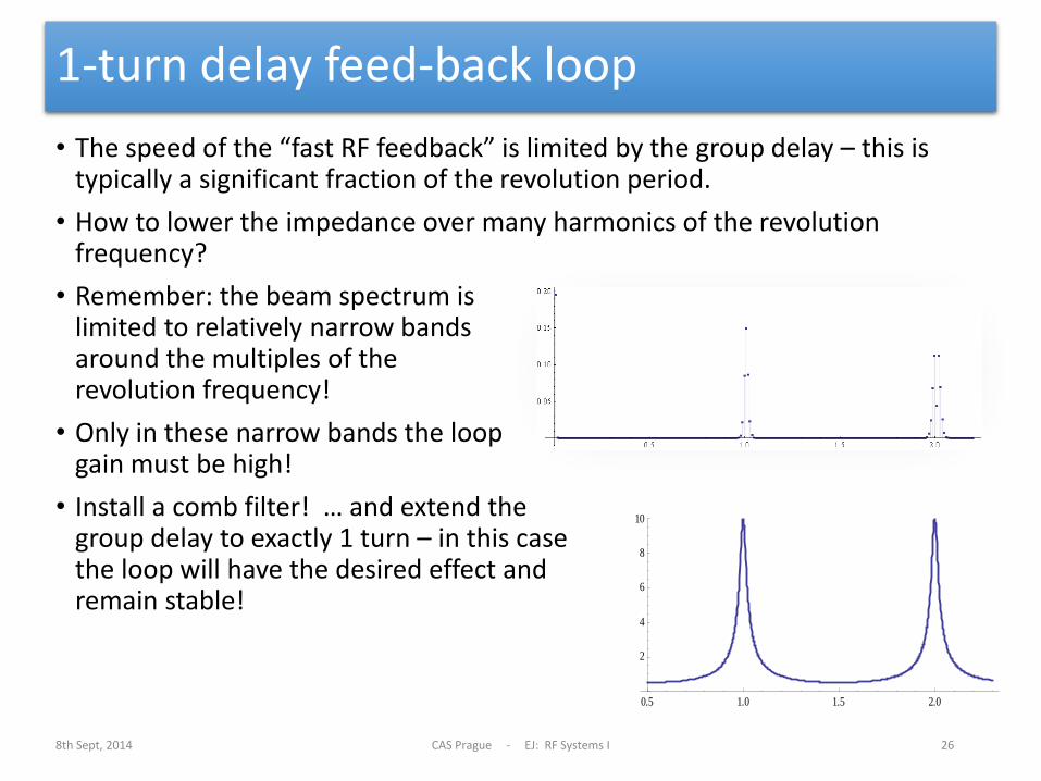
1-turn delay feed-back loop

• The speed of the “fast RF feedback” is limited by the group delay – this is typically a significant fraction of the revolution period.

• How to lower the impedance over many harmonics of the revolution frequency?

• Remember: the beam spectrum is limited to relatively narrow bands around the multiples of the revolution frequency!

• Only in these narrow bands the loop gain must be high!

• Install a comb filter! … and extend the group delay to exactly 1 turn – in this case the loop will have the desired effect and remain stable!


0.5 1.0 1.5 2.0

2

4

6

8

10

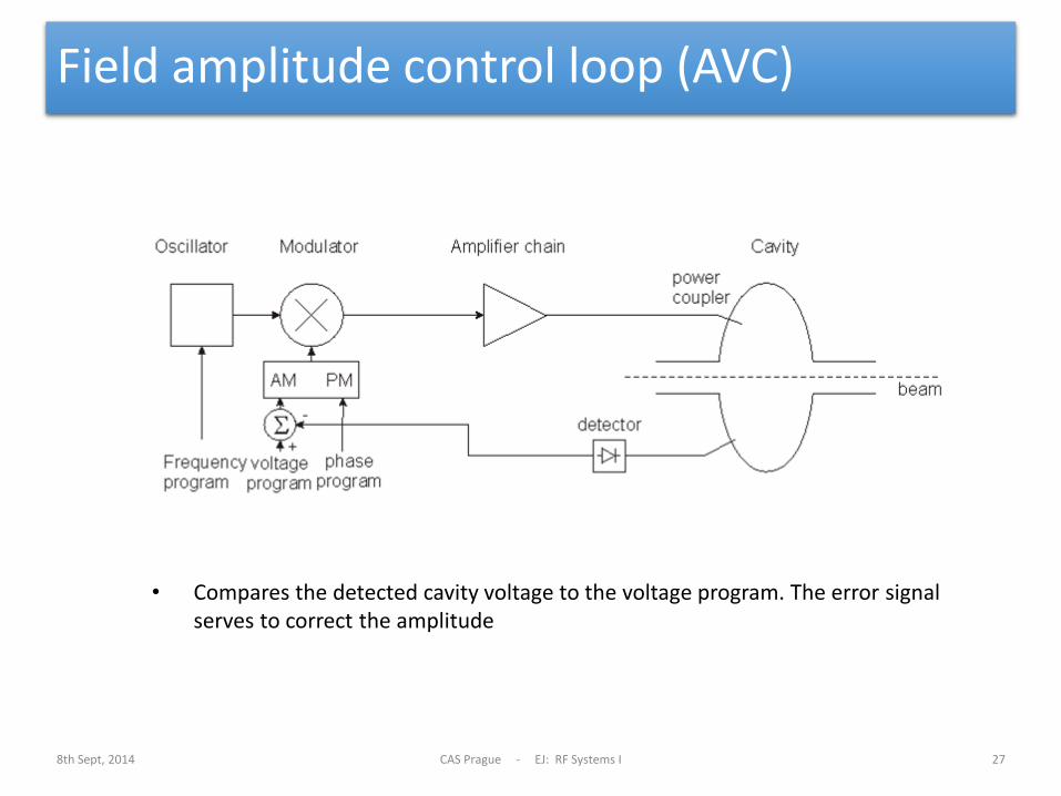
Field amplitude control loop (AVC)


• Compares the detected cavity voltage to the voltage program. The error signal serves to correct the amplitude

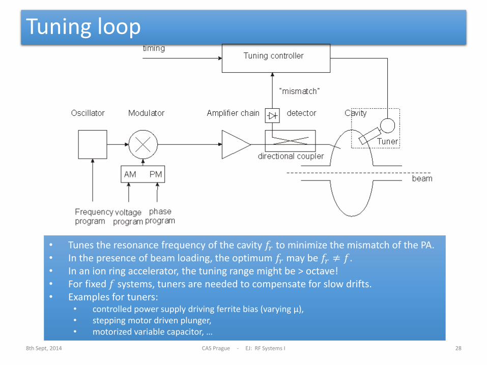
Tuning loop


• Tunes the resonance frequency of the cavity 𝑓𝑟 to minimize the mismatch of the PA. • In the presence of beam loading, the optimum 𝑓𝑟 may be 𝑓𝑟 ≠ 𝑓. • In an ion ring accelerator, the tuning range might be > octave! • For fixed 𝑓 systems, tuners are needed to compensate for slow drifts. • Examples for tuners:

• controlled power supply driving ferrite bias (varying µ), • stepping motor driven plunger, • motorized variable capacitor, …

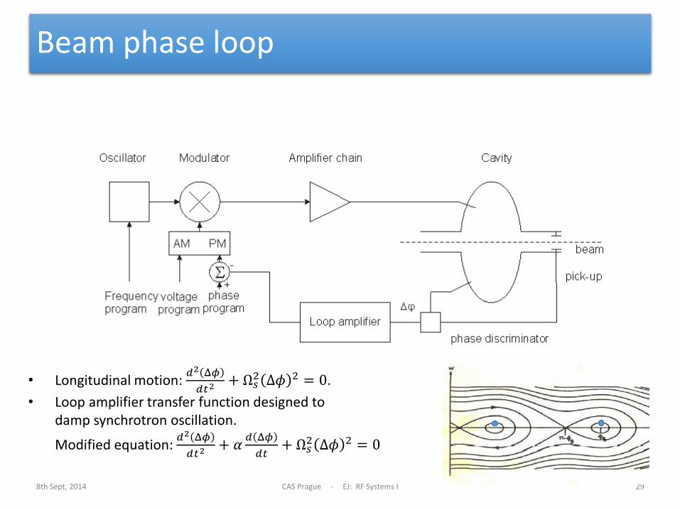
Beam phase loop


• Longitudinal motion: 𝑑2 Δ𝜙

𝑑𝑡2 + Ω𝑠2 Δ𝜙 2 = 0.

• Loop amplifier transfer function designed to damp synchrotron oscillation.

Modified equation: 𝑑2 Δ𝜙

𝑑𝑡2 + 𝛼𝑑 Δ𝜙

𝑑𝑡+ Ω𝑠

2 Δ𝜙 2 = 0

Other loops

• Radial loop: • Detect average radial position of the beam, • Compare to a programmed radial position, • Error signal controls the frequency.

• Synchronisation loop (e.g. before ejection): • 1st step: Synchronize 𝑓 to an external frequency (will also act

on radial position!). • 2nd step: phase loop brings bunches to correct position.

• …


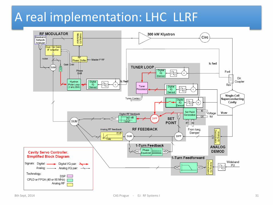
A real implementation: LHC LLRF


Fields in a waveguide


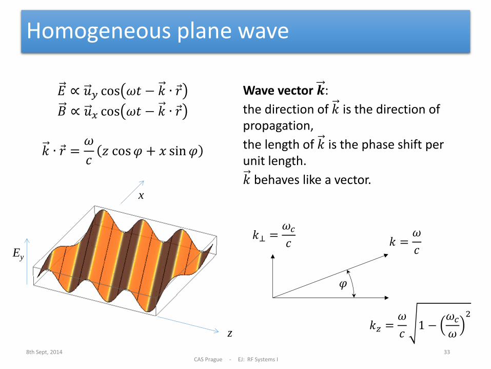
Wave vector 𝒌:

the direction of 𝑘 is the direction of propagation,

the length of 𝑘 is the phase shift per unit length.

𝑘 behaves like a vector.

Homogeneous plane wave


33

z

x

Ey

𝐸 ∝ 𝑢𝑦 cos 𝜔𝑡 − 𝑘 ∙ 𝑟

𝐵 ∝ 𝑢𝑥 cos 𝜔𝑡 − 𝑘 ∙ 𝑟

𝑘 ∙ 𝑟 =𝜔

𝑐𝑧 cos𝜑 + 𝑥 sin𝜑

𝑘⊥ =𝜔𝑐

𝑐

𝑘𝑧 =𝜔

𝑐1 −

𝜔𝑐

𝜔

2

𝑘 =𝜔

𝑐

𝜑

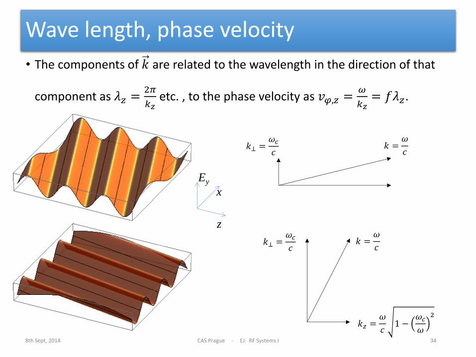
Wave length, phase velocity

• The components of 𝑘 are related to the wavelength in the direction of that

component as 𝜆𝑧 =2𝜋

𝑘𝑧 etc. , to the phase velocity as 𝑣𝜑,𝑧 =

𝜔

𝑘𝑧= 𝑓𝜆𝑧.


z

x

Ey

𝑘⊥ =𝜔𝑐

𝑐 𝑘 =

𝜔

𝑐

𝑘⊥ =𝜔𝑐

𝑐

𝑘𝑧 =𝜔

𝑐1 −

𝜔𝑐

𝜔

2

𝑘 =𝜔

𝑐

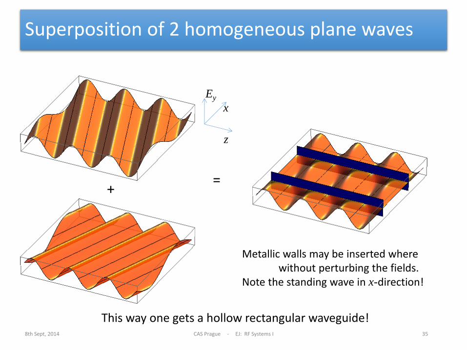
Superposition of 2 homogeneous plane waves


+ =

Metallic walls may be inserted where without perturbing the fields. Note the standing wave in x-direction!

z

x

Ey

This way one gets a hollow rectangular waveguide!

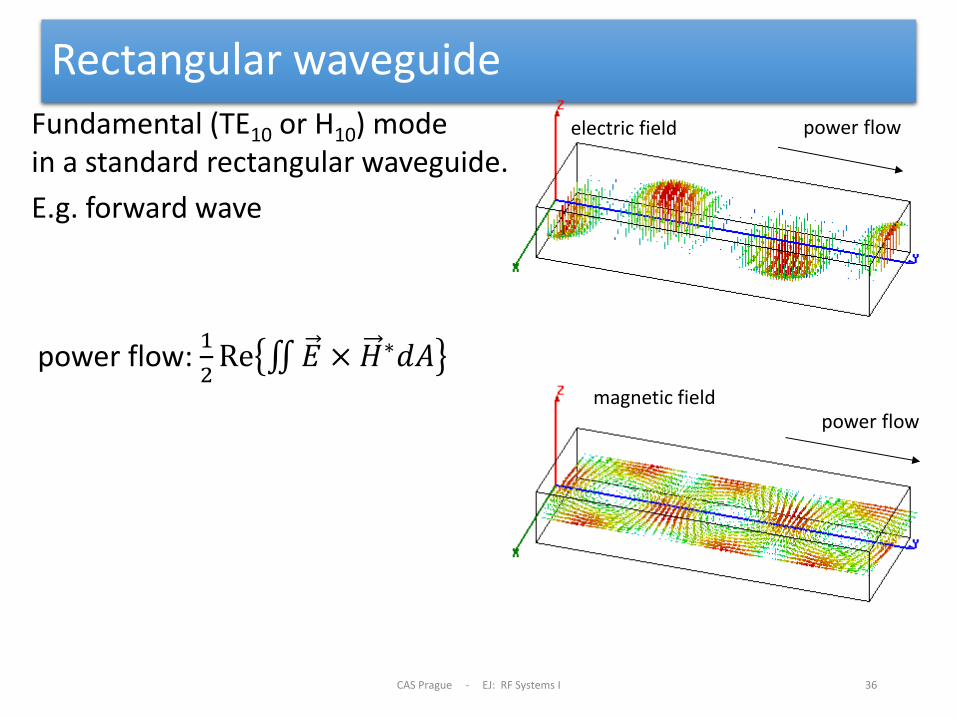
Rectangular waveguide

CAS Prague - EJ: RF Systems I 36

power flow: 1

2Re 𝐸 × 𝐻∗𝑑𝐴

Fundamental (TE10 or H10) mode in a standard rectangular waveguide.

E.g. forward wave

electric field

magnetic field

power flow

power flow

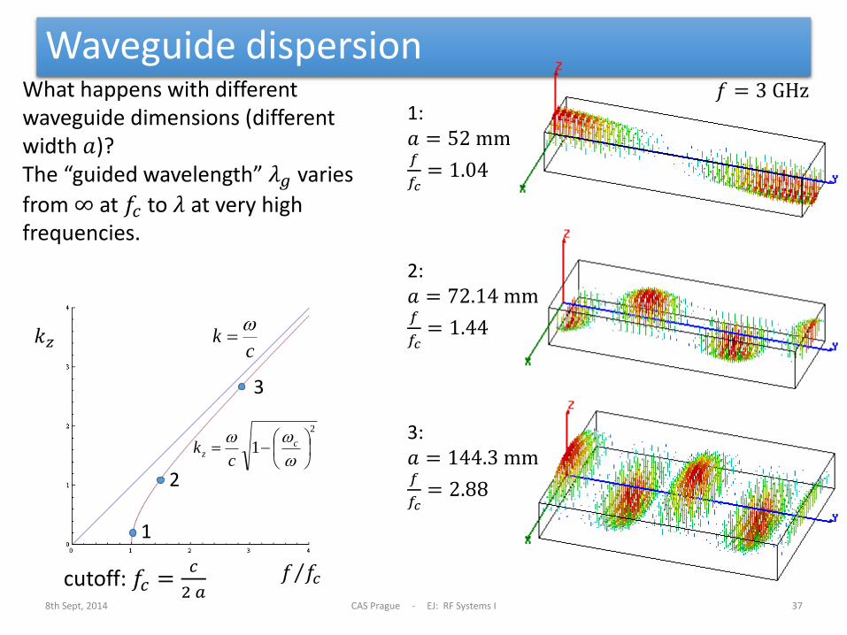
Waveguide dispersion


What happens with different waveguide dimensions (different width 𝑎)? The “guided wavelength” 𝜆𝑔 varies

from ∞ at 𝑓𝑐 to 𝜆 at very high frequencies.

cutoff: 𝑓𝑐 =𝑐

2 𝑎

2

1

cz

ck

ck

1

2

3

1: 𝑎 = 52 mm 𝑓

𝑓𝑐= 1.04

𝑓 = 3 GHz

2: 𝑎 = 72.14 mm 𝑓

𝑓𝑐= 1.44

3: 𝑎 = 144.3 mm 𝑓

𝑓𝑐= 2.88

𝑓 𝑓𝑐

𝑘𝑧

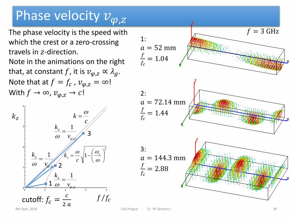
Phase velocity 𝑣𝜑,𝑧


2

1

cz

ck

ck

1

2

3

The phase velocity is the speed with which the crest or a zero-crossing travels in 𝑧-direction. Note in the animations on the right that, at constant 𝑓, it is 𝑣𝜑,𝑧 ∝ 𝜆𝑔.

Note that at 𝑓 = 𝑓𝑐 , 𝑣𝜑,𝑧 = ∞!

With 𝑓 → ∞, 𝑣𝜑,𝑧 → 𝑐!

z

z

v

k

,

1

z

z

v

k

,

1

z

z

v

k

,

1

1: 𝑎 = 52 mm 𝑓

𝑓𝑐= 1.04

𝑓 = 3 GHz

2: 𝑎 = 72.14 mm 𝑓

𝑓𝑐= 1.44

3: 𝑎 = 144.3 mm 𝑓

𝑓𝑐= 2.88

cutoff: 𝑓𝑐 =𝑐

2 𝑎 𝑓 𝑓𝑐

𝑘𝑧

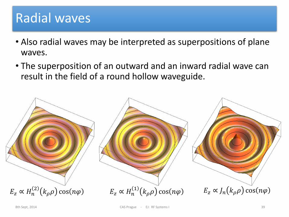
Radial waves

• Also radial waves may be interpreted as superpositions of plane waves.

• The superposition of an outward and an inward radial wave can result in the field of a round hollow waveguide.


𝐸𝑧 ∝ 𝐻𝑛2

𝑘𝜌𝜌 cos 𝑛𝜑 𝐸𝑧 ∝ 𝐻𝑛1

𝑘𝜌𝜌 cos 𝑛𝜑 𝐸𝑧 ∝ 𝐽𝑛 𝑘𝜌𝜌 cos 𝑛𝜑

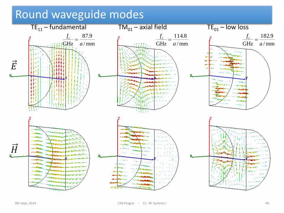
Round waveguide modes


TE11 – fundamental

mm/

9.87

GHz a

fc mm/

8.114

GHz a

fc mm/

9.182

GHz a

fc

TM01 – axial field TE01 – low loss

𝐸

𝐻

From waveguide to cavity


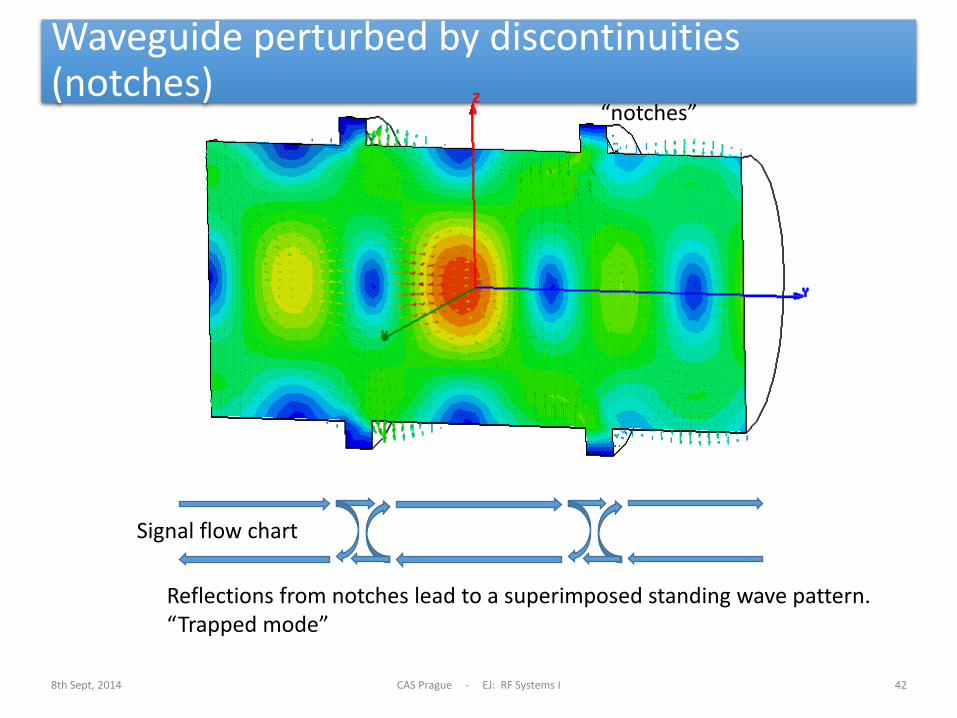
Waveguide perturbed by discontinuities (notches)


“notches”

Reflections from notches lead to a superimposed standing wave pattern. “Trapped mode”

Signal flow chart

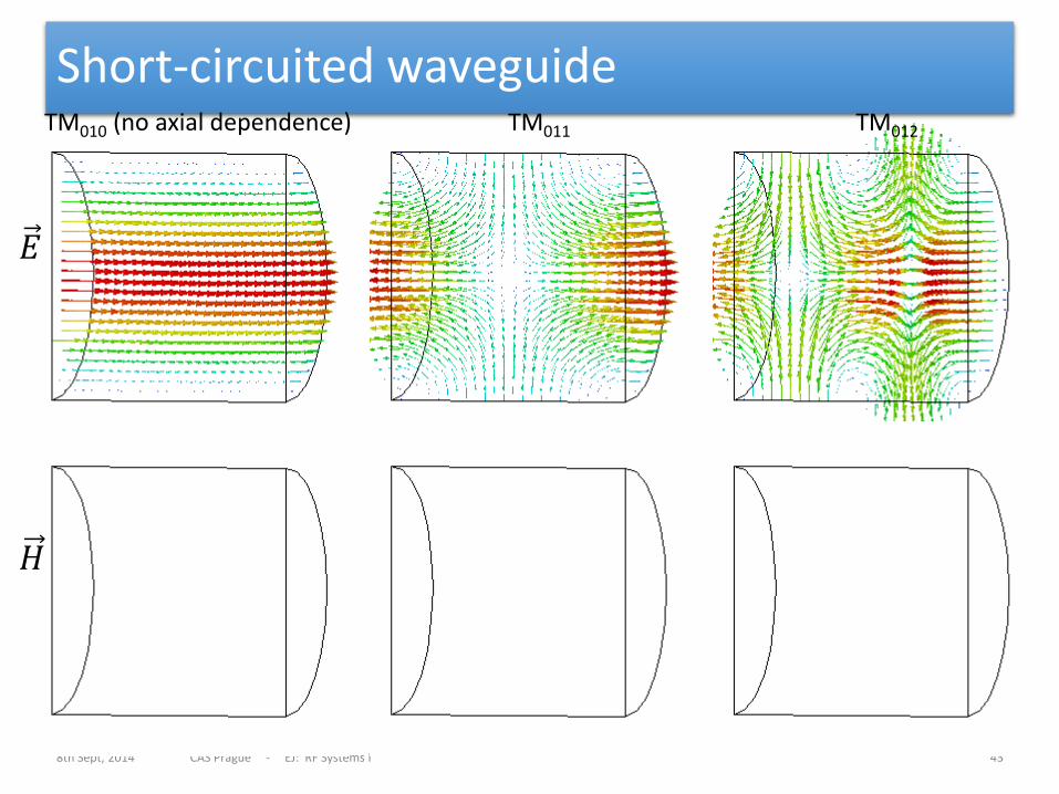
Short-circuited waveguide


TM010 (no axial dependence) TM011 TM012

𝐸

𝐻

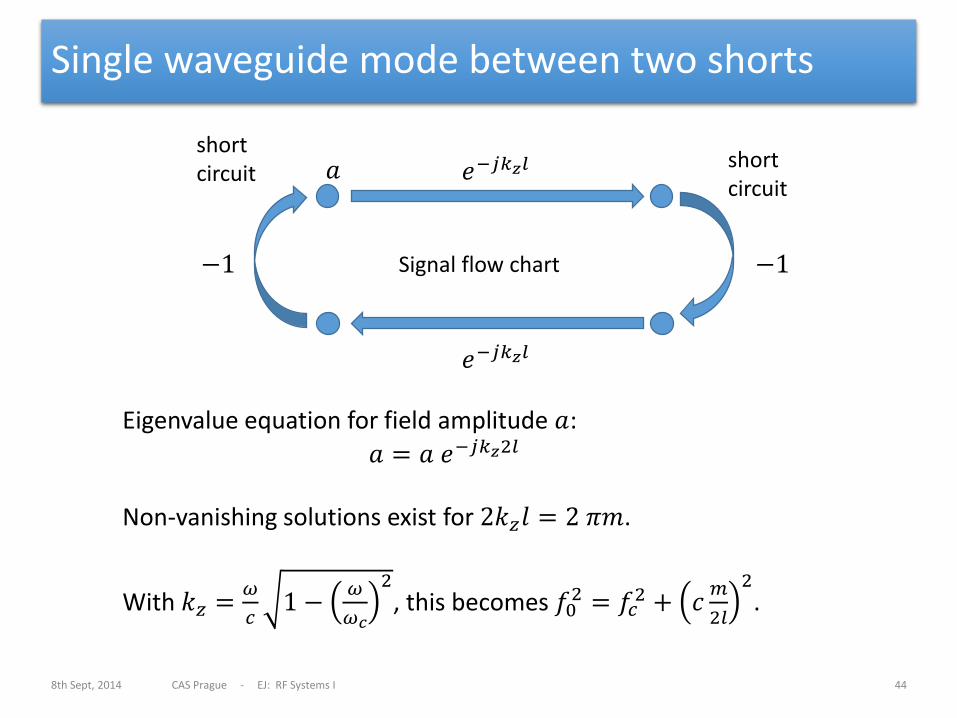
Single waveguide mode between two shorts


short circuit

short circuit

Eigenvalue equation for field amplitude 𝑎:

𝑎 = 𝑎 ⅇ−ⅉ𝑘𝑧2𝑙 Non-vanishing solutions exist for 2𝑘𝑧𝑙 = 2 𝜋𝑚.

With 𝑘𝑧 =𝜔

𝑐1 −

𝜔

𝜔𝑐

2, this becomes 𝑓0

2 = 𝑓𝑐2 + 𝑐

𝑚

2𝑙

2.

Signal flow chart

ⅇ−ⅉ𝑘𝑧𝑙

ⅇ−ⅉ𝑘𝑧𝑙

−1 −1

𝑎

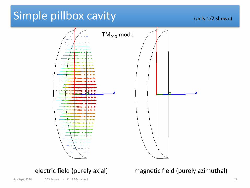
Simple pillbox cavity


electric field (purely axial) magnetic field (purely azimuthal)

(only 1/2 shown)

TM010-mode

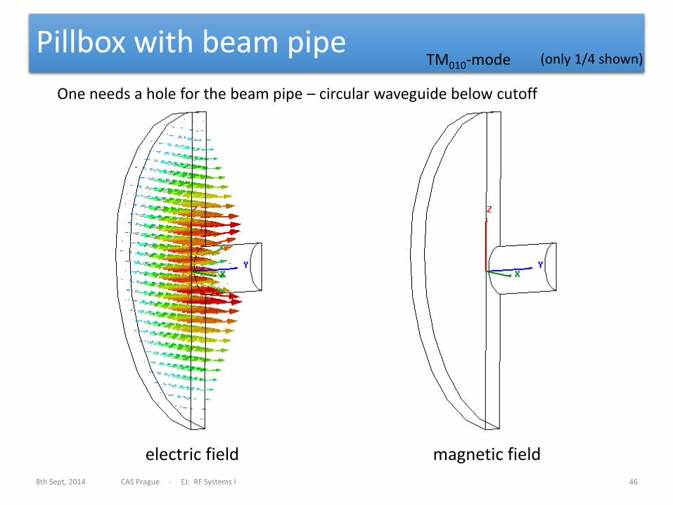
Pillbox with beam pipe


electric field magnetic field

(only 1/4 shown) TM010-mode

One needs a hole for the beam pipe – circular waveguide below cutoff

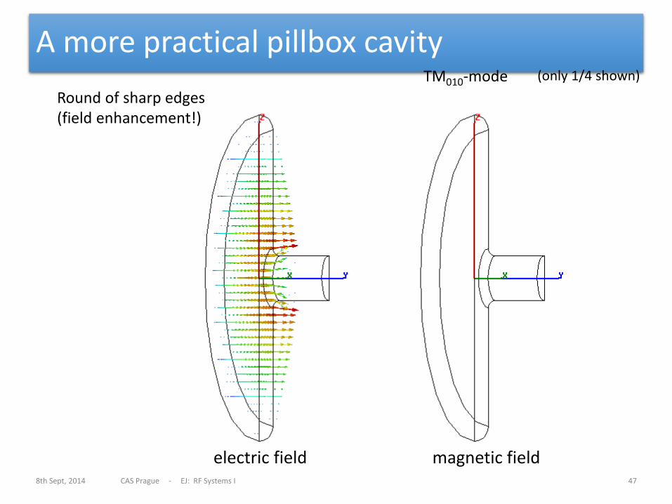
A more practical pillbox cavity


electric field magnetic field

(only 1/4 shown) TM010-mode

Round of sharp edges (field enhancement!)

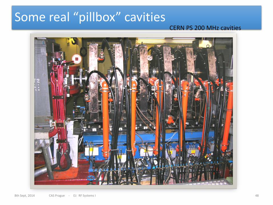
Some real “pillbox” cavities


CERN PS 200 MHz cavities

End of RF Systems I


RF Systems I - cas.web.cern.ch delay of 𝜏 becomes ... So I and Q are the Cartesian coordinates in...

Documents

Transcript of RF Systems I - cas.web.cern.ch delay of 𝜏 becomes ... So I and Q are the Cartesian coordinates in...