Optimizing the Conditions for Residual Stress Measurement...

Advances in Materials Physics and Chemistry, 2013, 3, 8-18 http://dx.doi.org/10.4236/ampc.2013.31A002 Published Online April 2013 (http://www.scirp.org/journal/ampc)

Optimizing the Conditions for Residual Stress Measurement Using a Two-Dimensional XRD Method with

Specimen Oscillation

Osamu Takakuwa, Hitoshi Soyama Department of Nanomechanics, Graduate School of Engineering, Tohoku University, Sendai, Japan

Email: [email protected]

Received January 14, 2013; revised February 25, 2013; accepted April 1, 2013

Copyright © 2013 Osamu Takakuwa, Hitoshi Soyama. This is an open access article distributed under the Creative Commons Attri-bution License, which permits unrestricted use, distribution, and reproduction in any medium, provided the original work is properly cited.

ABSTRACT

In order to optimize the conditions for residual stress measurement using a two-dimensional X-ray diffraction (2D-XRD) in terms of both efficiency and accuracy. The measurements have been conducted on three stainless steel specimens in this study. The three specimens were processed by annealing, a cavitating jet in air and a disc grinder, with each method introducing different residual stresses at the surface. The specimens were oscillated in the ω-direction, representing a right-hand rotation of the specimen about the incident X-ray beam. The range of the oscillation, Δω, was varied and optimum Δω was determined. Moreover, combinations of the tilt angle between the specimen surface normal and the diffraction vector, ψ, with the rotation angle about its surface normal, φ, have been studied with a view to find the most optimum condition. The results show that the use of ω oscillations is an effective method for improving analysis accuracy, especially for large grain metals. The standard error rapidly decreased with increasing range of the ω oscillation, especially for the annealed specimen which generated strong diffraction spots due to its large grain size. Keywords: Two-Dimensional XRD; Diffraction Ring; Oscillation; Residual Stress; Stainless Steel

1. Introduction

X-ray diffraction (XRD) is an effective method for the measurement of residual stress in polycrystalline metals. Such measurements are important since residual stress affects the mechanical property of metallic materials, e.g., resistance to fatigue strength [1-3], stress corrosion crack-ing [4] and hydrogen embrittlement [5-7]. The residual stress measurements need to be conducted with both high accuracy and efficiency both in the laboratory and in situations of practical application. Several XRD method- ologies have been developed so as to satisfy the needs mentioned above.

The sin2ψ method is one of the most simple and com- mon XRD methods for residual stress measurements and standardized approaches for this method have already been suggested [8,9]. On problem for the sin2ψ method, however, is that it is not easy to conduct accurate residual stress measurements for large grain metals when employing only a one-dimensional position sensitive pro- portional counter (PSPC) or scintillation counter. With such a detector only a few grains are irradiated resulting

in a sparse X-ray diffraction pattern and shortage of ψ angular information. In addition, the conventional sin2ψ method can measure residual stresses only in one direction per measurement and is therefore only really suitable for metals which do not have a complex stress field, i.e., not including shear stresses. In order to solve this problem, several studies have been conducted on the conventional sin2ψ method and based on these a useful additional methodology has been proposed for evaluating the biaxial stress including shear stress [10,11].

Recently, an XRD method for residual stress measurements using a two-dimensional PSPC (2D-PSPC) has been developed. The method focuses on the direct relationship between the stress tensor and diffraction conic section distortion [12]. The method is known as the two- dimensional XRD method (2D-XRD or XRD2). The 2D- XRD method can measure six components of the stress tensor, i.e., biaxial stress, including shear stress, from the direct relationship between the stress tensor and the dis-tortion of the diffraction conic section obtained directly by the 2D-PSPC. Moreover, this method can also measure the local residual stress in textured material, weakly

Copyright © 2013 SciRes. AMPC

O. TAKAKUWA, H. SOYAMA 9

diffracting material and in regions of small area down to mm2, since the diffracted X-ray are efficiently detected by the 2D-PSPC.

The fundamentals and details of 2D-XRD have been described well in the literature [13,14] and in a book [15]. However a standard methodology for 2D-XRD has not been established yet, since this method has only been relatively recently applied to residual stress measurements. Therefore the precise conditions used for the measurement, e.g., the rotation angles and exposure times needed to detect the diffraction ring, need to be optimized. The overall optimization process needs to take into account both measurement efficiency and accuracy.

The diffracted X-ray from large grain materials, such as annealed specimens, produces strongly scattered spots in the X-ray diffraction profile and, consequently, a lack of accuracy in the residual stress measurement. This occurs even if the measurement time is prolonged. This can be a problem for the measurements using 2D-XRD. In order to solve this problem, an oscillatory method should be effective and indeed in the conventional sin2ψ method, an oscillation of the ψ angle is generally used. However when the ψ angle is oscillated, the range of this oscillation needs to be as small as possible because the incident angle about the lattice plane directly changes during the ψ oscillation. This affects the relationship between the diffraction angle and the ψ angle, i.e., the 2θ-sin2ψ relationship. For this reason an oscillation which keeps the ψ angle constant is more preferable.

In this paper residual stress measurements using the 2D-XRD method have been carried out on three specimens made of stainless steel in order to optimize several of the conditions for residual stress measurements, e.g., sample rotation angles and exposure time, with respect to both measurement efficiency and accuracy. The specimens had three types of residual stress as follows: a low stress value with a large grain (by Annealing), an equibiaxial compressive residual stress (by Cavitating jet in air) and an anisotropic tensile residual stress (by Disc grinder). The conditions for the stress measurements were optimized, in terms of the detection time and the number of diffraction ring measurements taken from various angles of the specimen. The optimization process took into account the achievement of both high accuracy and good measurement efficiency.

2. Experimental Apparatus and Procedures

2.1. Introduction of Various Residual Stresses

The material under test was made of JIS SUS316L austenitic stainless steel. The geometry and dimensions of the specimen were 35 mm square and 3 mm thick. Three types of treatment were chosen which introduce different residual stresses into the specimens. The specimens were

prepared by annealing, the use of a cavitating jet in air and by using a disc grinder. The annealing treatment re- leases residual stresses introduced by shape forming and increases the grain size. The use of a cavitating jet in air introduces high equibiaxial compressive residual stresses into the surface layer by impacts due to cavitation bubble collapse. The method is highly effective and has now been applied for practical usage. The disc grinder is one of a number of surface finishing methods that are fre- quently applied to metals. Its characteristics are that it introduces high anisotropic tensile residual stress at the near surface of the specimen. For the annealed specimen, the sample was heated at 1000 degree Celsius for 1 h, and then furnace cooled. For the specimen prepared us-ing a cavitating jet in air, the conditions for the treatment were same as previously reported [16,17] and for this treatment the processing time per unit length was 1 s/mm. For the sample prepared using the disc grinder, the rota-tion speed was set to 11,000 rpm and the disc, manufac-tured by NIPPON RESIBON COOPRATION (A/W36P), had a diameter of 100 mm. The direction of residual stress caused by the disc grinder was defined by the ro-tating and the scanning direction of the disc as x and y, respectively. After the preparation of the specimens, residual stress measurements were carried out in accor- dance with following conditions.

2.2. Residual Stress Measurements

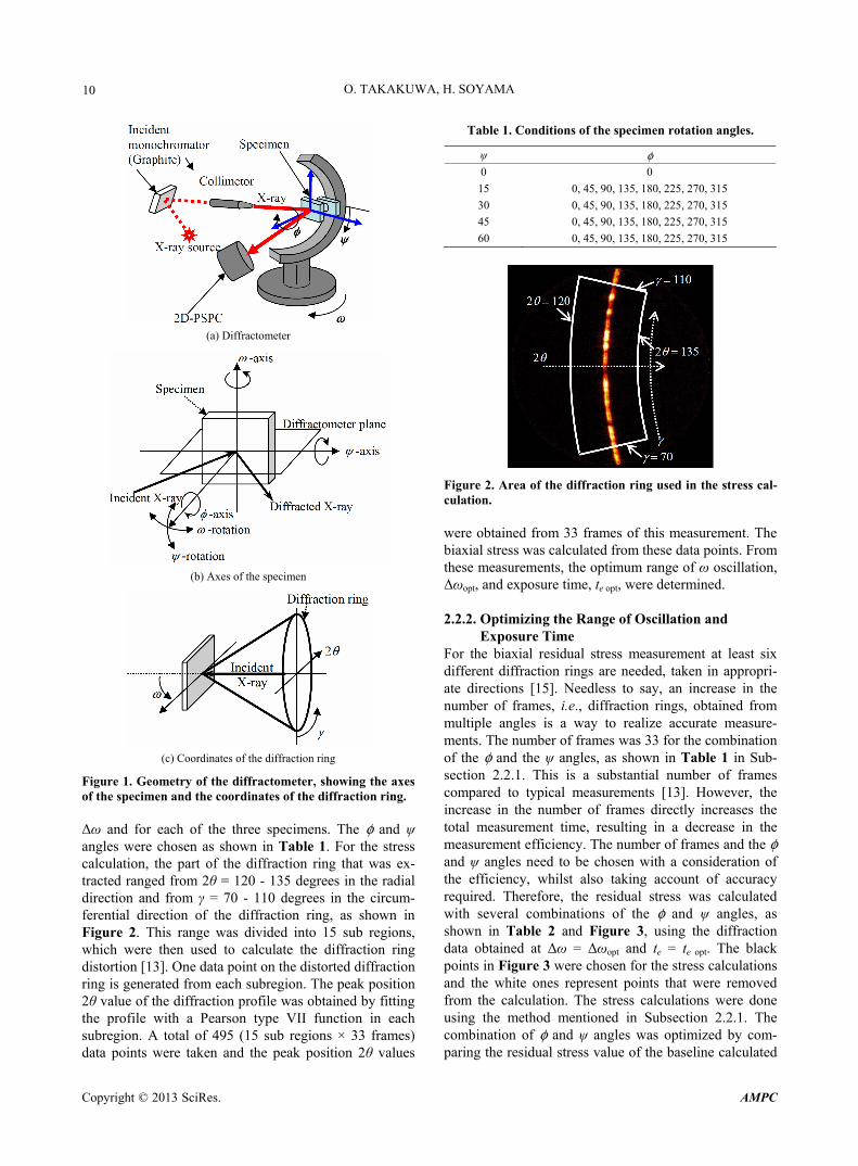
The X-ray diffraction measurements were carried out using Cr Ka X-rays from a tube operated at 35 kV and 40 mA through a 0.5 mm diameter total reflection collimetor and with an incident monochromator (D8 DISCOVER, Bruker AXS Inc.). The lattice plane, (h k l), used was the γ-Fe (2 2 0) plane and the diffraction angle without strain was 128 degrees. The specimen was placed in a diffractometer, the geometry of which is shown in Figure 1. The diffraction ring from the specimen was detected at several angles by the 2D-PSPC, with the angles denoted as φ and ψ as shown on the figures. These angular values were used to calculate the stress tensor. The fundamen-tals of the calculation of biaxial stress using the 2D-XRD method are described in detail in ref [15].

2.2.1. Optimizing the Range of Oscillation and Exposure Time

An initial ω angle of 110 degrees was chosen and the specimen was oscillated over a range of Δω during the measurement. The parameter Δω was varied between 0 (without oscillation) and 2, 4, 6, 8 and 10 degrees in order to verify the effect of the ω oscillation on the diffrac-tion ring and ultimately on the stress calculation. In addition, the exposure time per frame for the detection of the diffraction ring at a single position (φ, ψ), te, was also varied as te = 60, 90, 120, 150 and 180 sec for each value of



(a) Diffractometer

(b) Axes of the specimen

(c) Coordinates of the diffraction ring

Figure 1. Geometry of the diffractometer, showing the axes of the specimen and the coordinates of the diffraction ring.

Δω and for each of the three specimens. The φ and ψ angles were chosen as shown in Table 1. For the stress calculation, the part of the diffraction ring that was ex-tracted ranged from 2θ = 120 - 135 degrees in the radial direction and from γ = 70 - 110 degrees in the circum-ferential direction of the diffraction ring, as shown in Figure 2. This range was divided into 15 sub regions, which were then used to calculate the diffraction ring distortion [13]. One data point on the distorted diffraction ring is generated from each subregion. The peak position 2θ value of the diffraction profile was obtained by fitting the profile with a Pearson type VII function in each subregion. A total of 495 (15 sub regions × 33 frames) data points were taken and the peak position 2θ values

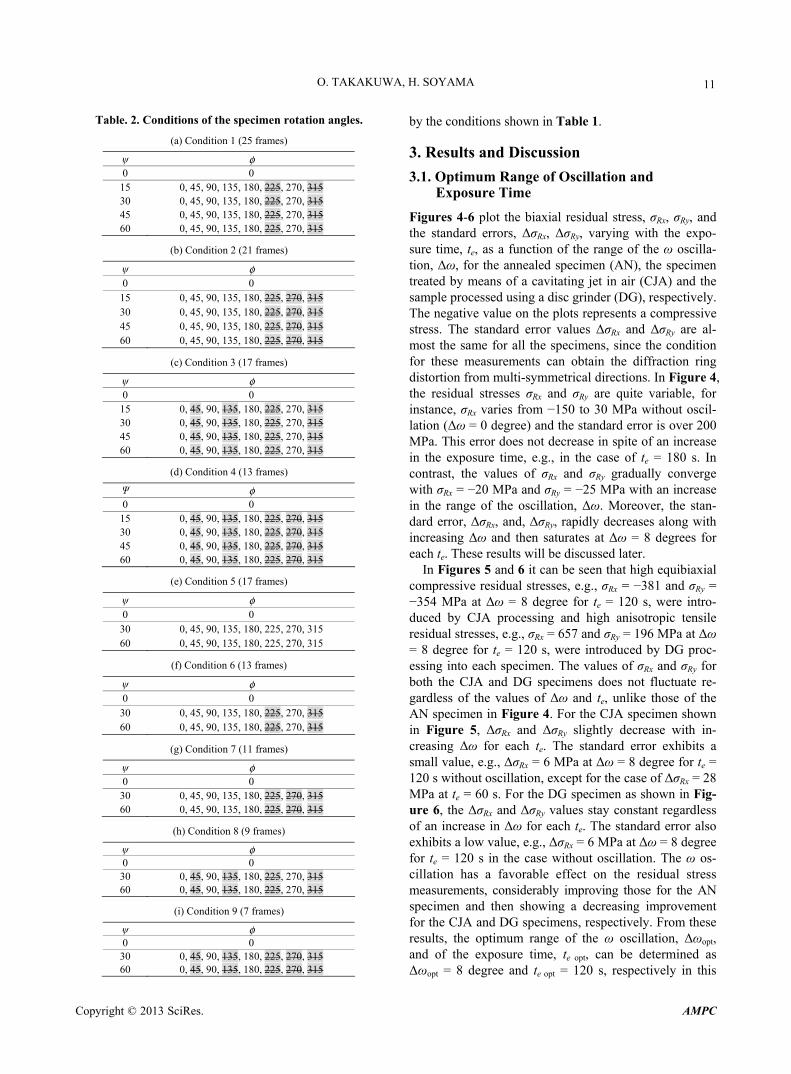
Table 1. Conditions of the specimen rotation angles.

ψ φ 0 0

15 0, 45, 90, 135, 180, 225, 270, 315

30 0, 45, 90, 135, 180, 225, 270, 315

45 0, 45, 90, 135, 180, 225, 270, 315

60 0, 45, 90, 135, 180, 225, 270, 315

Figure 2. Area of the diffraction ring used in the stress cal-culation.

were obtained from 33 frames of this measurement. The biaxial stress was calculated from these data points. From these measurements, the optimum range of ω oscillation, Δωopt, and exposure time, te opt, were determined.

2.2.2. Optimizing the Range of Oscillation and Exposure Time

For the biaxial residual stress measurement at least six different diffraction rings are needed, taken in appropri- ate directions [15]. Needless to say, an increase in the number of frames, i.e., diffraction rings, obtained from multiple angles is a way to realize accurate measurements. The number of frames was 33 for the combination of the φ and the ψ angles, as shown in Table 1 in Sub- section 2.2.1. This is a substantial number of frames compared to typical measurements [13]. However, the increase in the number of frames directly increases the total measurement time, resulting in a decrease in the measurement efficiency. The number of frames and the φ and ψ angles need to be chosen with a consideration of the efficiency, whilst also taking account of accuracy required. Therefore, the residual stress was calculated with several combinations of the φ and ψ angles, as shown in Table 2 and Figure 3, using the diffraction data obtained at Δω = Δωopt and te = te opt. The black points in Figure 3 were chosen for the stress calculations and the white ones represent points that were removed from the calculation. The stress calculations were done using the method mentioned in Subsection 2.2.1. The combination of φ and ψ angles was optimized by com-paring the residual stress value of the baseline calculated



Table. 2. Conditions of the specimen rotation angles.

(a) Condition 1 (25 frames)

ψ φ 0 0

15 0, 45, 90, 135, 180, 225, 270, 315 30 0, 45, 90, 135, 180, 225, 270, 315 45 0, 45, 90, 135, 180, 225, 270, 315 60 0, 45, 90, 135, 180, 225, 270, 315

(b) Condition 2 (21 frames)

ψ φ 0 0

15 0, 45, 90, 135, 180, 225, 270, 315 30 0, 45, 90, 135, 180, 225, 270, 315 45 0, 45, 90, 135, 180, 225, 270, 315 60 0, 45, 90, 135, 180, 225, 270, 315

(c) Condition 3 (17 frames)

ψ φ 0 0

15 0, 45, 90, 135, 180, 225, 270, 315 30 0, 45, 90, 135, 180, 225, 270, 315 45 0, 45, 90, 135, 180, 225, 270, 315 60 0, 45, 90, 135, 180, 225, 270, 315

(d) Condition 4 (13 frames)

Ψ φ 0 0

15 0, 45, 90, 135, 180, 225, 270, 315 30 0, 45, 90, 135, 180, 225, 270, 315 45 0, 45, 90, 135, 180, 225, 270, 315 60 0, 45, 90, 135, 180, 225, 270, 315

(e) Condition 5 (17 frames)

ψ φ 0 0

30 0, 45, 90, 135, 180, 225, 270, 315 60 0, 45, 90, 135, 180, 225, 270, 315

(f) Condition 6 (13 frames)

ψ φ 0 0

30 0, 45, 90, 135, 180, 225, 270, 315 60 0, 45, 90, 135, 180, 225, 270, 315

(g) Condition 7 (11 frames)

ψ φ 0 0

30 0, 45, 90, 135, 180, 225, 270, 315 60 0, 45, 90, 135, 180, 225, 270, 315

(h) Condition 8 (9 frames)

ψ φ 0 0

30 0, 45, 90, 135, 180, 225, 270, 315 60 0, 45, 90, 135, 180, 225, 270, 315

(i) Condition 9 (7 frames)

ψ φ 0 0

30 0, 45, 90, 135, 180, 225, 270, 315 60 0, 45, 90, 135, 180, 225, 270, 315

by the conditions shown in Table 1.

3. Results and Discussion

3.1. Optimum Range of Oscillation and Exposure Time

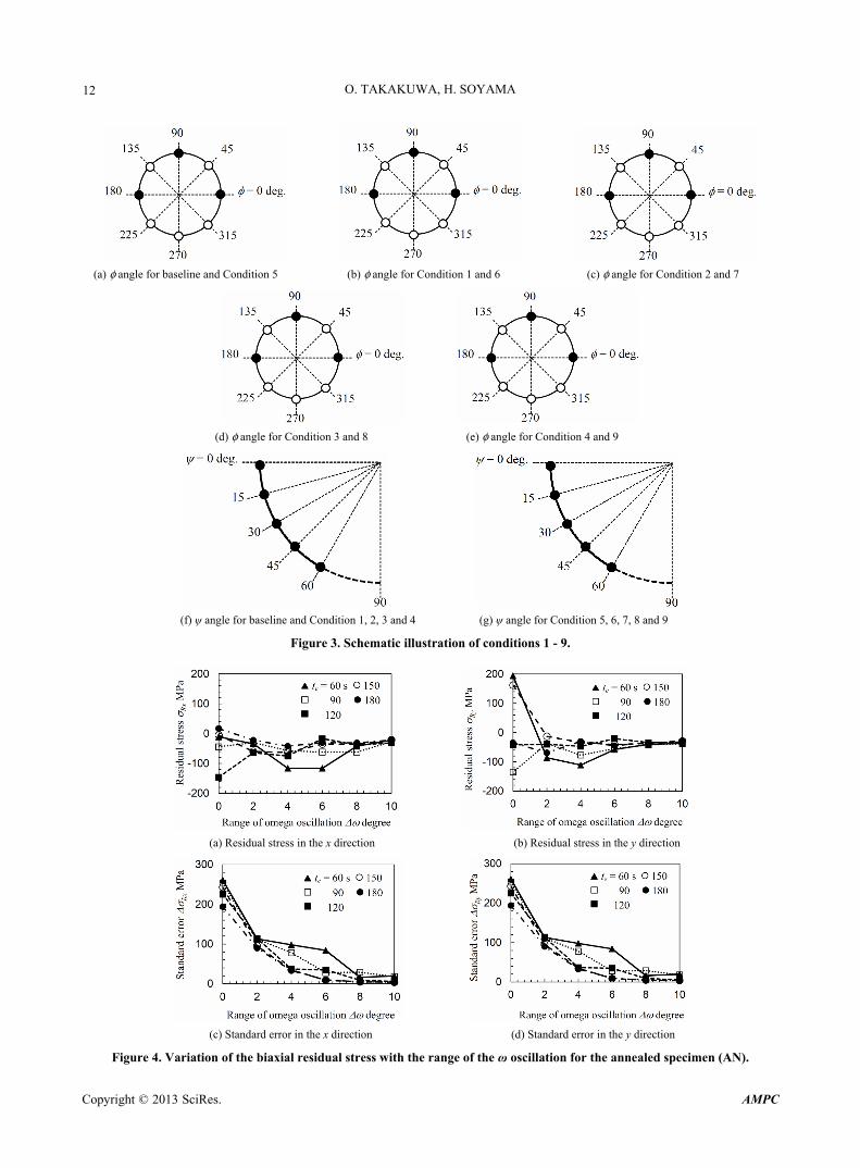
Figures 4-6 plot the biaxial residual stress, σRx, σRy, and the standard errors, ΔσRx, ΔσRy, varying with the exposure time, te, as a function of the range of the ω oscillation, Δω, for the annealed specimen (AN), the specimen treated by means of a cavitating jet in air (CJA) and the sample processed using a disc grinder (DG), respectively. The negative value on the plots represents a compressive stress. The standard error values ΔσRx and ΔσRy are al- most the same for all the specimens, since the condition for these measurements can obtain the diffraction ring distortion from multi-symmetrical directions. In Figure 4, the residual stresses σRx and σRy are quite variable, for instance, σRx varies from −150 to 30 MPa without oscillation (Δω = 0 degree) and the standard error is over 200 MPa. This error does not decrease in spite of an increase in the exposure time, e.g., in the case of te = 180 s. In contrast, the values of σRx and σRy gradually converge with σRx = −20 MPa and σRy = −25 MPa with an increase in the range of the oscillation, Δω. Moreover, the stan-dard error, ΔσRx, and, ΔσRy, rapidly decreases along with increasing Δω and then saturates at Δω = 8 degrees for each te. These results will be discussed later.

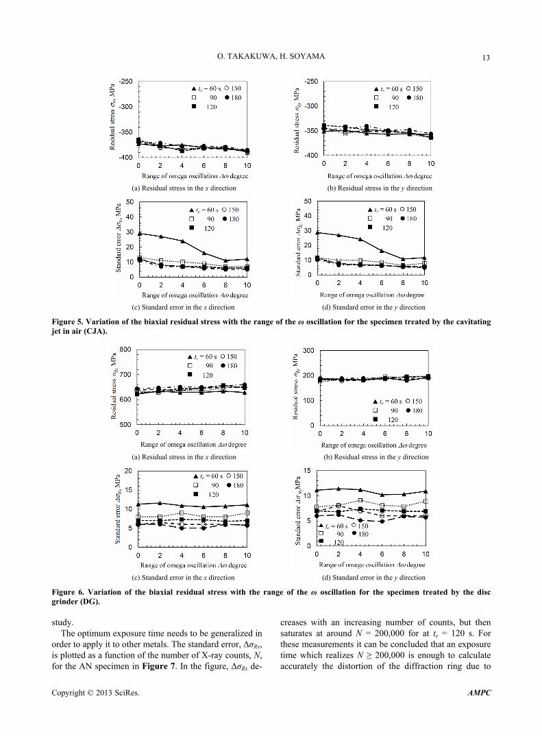
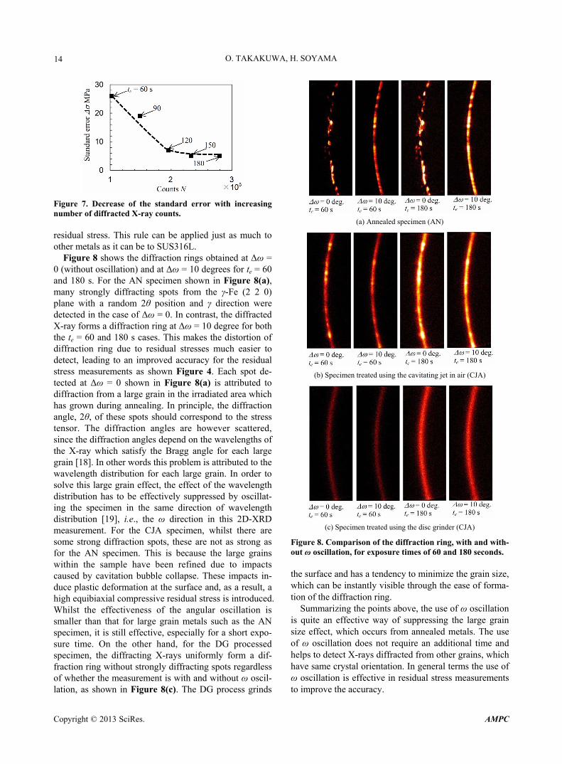
In Figures 5 and 6 it can be seen that high equibiaxial compressive residual stresses, e.g., σRx = −381 and σRy = −354 MPa at Δω = 8 degree for te = 120 s, were intro-duced by CJA processing and high anisotropic tensile residual stresses, e.g., σRx = 657 and σRy = 196 MPa at Δω = 8 degree for te = 120 s, were introduced by DG proc-essing into each specimen. The values of σRx and σRy for both the CJA and DG specimens does not fluctuate re-gardless of the values of Δω and te, unlike those of the AN specimen in Figure 4. For the CJA specimen shown in Figure 5, ΔσRx and ΔσRy slightly decrease with increasing Δω for each te. The standard error exhibits a small value, e.g., ΔσRx = 6 MPa at Δω = 8 degree for te = 120 s without oscillation, except for the case of ΔσRx = 28 MPa at te = 60 s. For the DG specimen as shown in Fig- ure 6, the ΔσRx and ΔσRy values stay constant regardless of an increase in Δω for each te. The standard error also exhibits a low value, e.g., ΔσRx = 6 MPa at Δω = 8 degree for te = 120 s in the case without oscillation. The ω oscillation has a favorable effect on the residual stress measurements, considerably improving those for the AN specimen and then showing a decreasing improvement for the CJA and DG specimens, respectively. From these results, the optimum range of the ω oscillation, Δωopt, and of the exposure time, te opt, can be determined as Δωopt = 8 degree and te opt = 120 s, respectively in this


O. TAKAKUWA, H. SOYAMA


12

(a) φ angle for baseline and Condition 5 (b) φ angle for Condition 1 and 6 (c) φ angle for Condition 2 and 7

(d) φ angle for Condition 3 and 8 (e) φ angle for Condition 4 and 9

(f) ψ angle for baseline and Condition 1, 2, 3 and 4 (g) ψ angle for Condition 5, 6, 7, 8 and 9

Figure 3. Schematic illustration of conditions 1 - 9.

(a) Residual stress in the x direction (b) Residual stress in the y direction

(c) Standard error in the x direction (d) Standard error in the y direction

Figure 4. Variation of the biaxial residual stress with the range of the ω oscillation for the annealed specimen (AN).




Figure 5. Variation of the biaxial residual stress with the range of the ω oscillation for the specimen treated by the cavitating jet in air (CJA).



Figure 6. Variation of the biaxial residual stress with the range of the ω oscillation for the specimen treated by the disc grinder (DG).

study.

The optimum exposure time needs to be generalized in order to apply it to other metals. The standard error, ΔσRx, is plotted as a function of the number of X-ray counts, N, for the AN specimen in Figure 7. In the figure, ΔσRx de-

creases with an increasing number of counts, but then saturates at around N = 200,000 for at te = 120 s. For these measurements it can be concluded that an exposure time which realizes N ≥ 200,000 is enough to calculate accurately the distortion of the diffraction ring due to



Figure 7. Decrease of the standard error with increasing number of diffracted X-ray counts.

residual stress. This rule can be applied just as much to other metals as it can be to SUS316L.

Figure 8 shows the diffraction rings obtained at Δω = 0 (without oscillation) and at Δω = 10 degrees for te = 60 and 180 s. For the AN specimen shown in Figure 8(a), many strongly diffracting spots from the γ-Fe (2 2 0) plane with a random 2θ position and γ direction were detected in the case of Δω = 0. In contrast, the diffracted X-ray forms a diffraction ring at Δω = 10 degree for both the te = 60 and 180 s cases. This makes the distortion of diffraction ring due to residual stresses much easier to detect, leading to an improved accuracy for the residual stress measurements as shown Figure 4. Each spot de-tected at Δω = 0 shown in Figure 8(a) is attributed to diffraction from a large grain in the irradiated area which has grown during annealing. In principle, the diffraction angle, 2θ, of these spots should correspond to the stress tensor. The diffraction angles are however scattered, since the diffraction angles depend on the wavelengths of the X-ray which satisfy the Bragg angle for each large grain [18]. In other words this problem is attributed to the wavelength distribution for each large grain. In order to solve this large grain effect, the effect of the wavelength distribution has to be effectively suppressed by oscillat- ing the specimen in the same direction of wavelength distribution [19], i.e., the ω direction in this 2D-XRD measurement. For the CJA specimen, whilst there are some strong diffraction spots, these are not as strong as for the AN specimen. This is because the large grains within the sample have been refined due to impacts caused by cavitation bubble collapse. These impacts in- duce plastic deformation at the surface and, as a result, a high equibiaxial compressive residual stress is introduced. Whilst the effectiveness of the angular oscillation is smaller than that for large grain metals such as the AN specimen, it is still effective, especially for a short exposure time. On the other hand, for the DG processed specimen, the diffracting X-rays uniformly form a diffraction ring without strongly diffracting spots regardless of whether the measurement is with and without ω oscillation, as shown in Figure 8(c). The DG process grinds

(a) Annealed specimen (AN)

(b) Specimen treated using the cavitating jet in air (CJA)

(c) Specimen treated using the disc grinder (CJA)

Figure 8. Comparison of the diffraction ring, with and without ω oscillation, for exposure times of 60 and 180 seconds.

the surface and has a tendency to minimize the grain size, which can be instantly visible through the ease of forma- tion of the diffraction ring.

Summarizing the points above, the use of ω oscillation is quite an effective way of suppressing the large grain size effect, which occurs from annealed metals. The use of ω oscillation does not require an additional time and helps to detect X-rays diffracted from other grains, which have same crystal orientation. In general terms the use of ω oscillation is effective in residual stress measurements to improve the accuracy.



3.2. Optimum Angles of Specimen Rotation

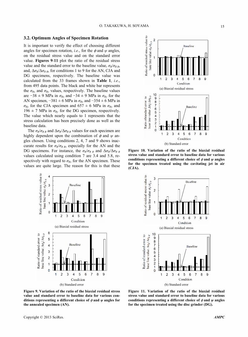
It is important to verify the effect of choosing different angles for specimen rotation, i.e., for the φ and ψ angles, on the residual stress value and on the standard error value. Figures 9-11 plot the ratio of the residual stress value and the standard error to the baseline value, σR/σR B, and, ΔσR/ΔσR B, for conditions 1 to 9 for the AN, CJA and DG specimens, respectively. The baseline value was calculated from the 33 frames shown in Table 1, i.e., from 495 data points. The black and white bar represents the σRx and σRy values, respectively. The baseline values are −38 ± 9 MPa in σRx and −34 ± 9 MPa in σRy for the AN specimen, −381 ± 6 MPa in σRx and −354 ± 6 MPa in σRy for the CJA specimen and 657 ± 6 MPa in σRx and 196 ± 7 MPa in σRy for the DG specimen, respectively. The value which nearly equals to 1 represents that the stress calculation has been precisely done as well as the baseline data.

The σR/σR B and ΔσR/ΔσR B values for each specimen are highly dependent upon the combination of φ and ψ angles chosen. Using conditions 2, 4, 7 and 9 shows inac- curate results for σR/σR B, especially for the AN and the DG specimens. For instance, the σR/σR B and ΔσR/ΔσR B values calculated using condition 7 are 3.4 and 5.8, respectively with regard to σRx for the AN specimen. These values are quite large. The reason for this is that these

(a) Biaxial residual stress

(b) Standard error

Figure 9. Variation of the ratio of the biaxial residual stress value and standard error to baseline data for various conditions representing a different choice of φ and ψ angles for the annealed specimen (AN).


(b) Standard error

Figure 10. Variation of the ratio of the biaxial residual stress value and standard error to baseline data for various conditions representing a different choice of φ and ψ angles for the specimen treated using the cavitating jet in air (CJA).


(b) Standard error

Figure 11. Variation of the ratio of the biaxial residual stress value and standard error to baseline data for various conditions representing a different choice of φ and ψ angles for the specimen treated using the disc grinder (DG).



conditions can obtain a diffraction ring from only one side, e.g., for φ = 0, 45, 90, 135 and 180 degrees in con-ditions 2 and 7. In contrast, accurate results for σR/σR B for each specimen are obtained using conditions 1, 3, 5, 6 and 8. This occurs since several angles of φ, which are not one-sided, were employed in these conditions, e.g., φ = 0, 90, 180, and 270 degrees for conditions 3 and 9. The general rule is that a lack of diffraction information from a opposite side causes variability in the determination of the stress vector. This effect appears in any stress direc-tion and depends precise combination of ω, φ and ψ an-gles used [15]. Moreover, this effect becomes smaller when the residual stress measurements are carried out to assess equibiaxial stress fields such as that found in the CJA specimen, since the diffraction ring is distorted symmetrically due to the equibiaxial stress field. In order to choose the optimum conditions, several comparisons will be made regarding conditions 1, 3, 5, 6 and 8 in the following paragraph.

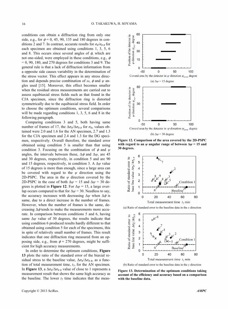
Comparing conditions 3 and 5, both having same number of frames of 17, the ΔσR/ΔσR B for σRx values obtained were 2.0 and 1.6 for the AN specimen, 2.7 and 1.3 for the CJA specimen and 2.4 and 1.3 for the DG specimen, respectively. Overall therefore, the standard error obtained using condition 5 is smaller than that using condition 3. Focusing on the combination of φ and ψ angles, the intervals between these, Δφ and Δψ, are 45 and 30 degrees, respectively, in condition 5 and are 90 and 15 degrees, respectively, in condition 3. A Δψ value of 15 degrees is more than enough, since a large area can be covered with regard to the ψ direction using the 2D-PSPC. The area in the ψ direction covered by the 2D-PSPC in the case of both Δψ = 15 and Δψ = 30 degrees is plotted in Figure 12. For Δψ = 15, a large over- lap occurs compared to that for Δψ = 30. Needless to say, the accuracy increases with decreasing Δψ when Δφ is same, due to a direct increase in the number of frames. However, when the number of frames is the same, decreasing Δφ tends to make the measurements more accurate. In comparison between conditions 5 and 6, having same Δψ value of 30 degrees, the results indicate that using condition 6 produced results hardly different to that obtained using condition 5 for each of the specimens, this in spite of relatively small number of frames. This result indicates that one diffraction ring measured from an op- posing side, e.g., from φ = 270 degrees, might be suffi-cient for high accuracy measurements.

In order to determine the optimum conditions, Figure 13 plots the ratio of the standard error of the biaxial residual stress to the baseline value, ΔσR/ΔσR B, as a function of total measurement time, tT, for the AN specimen. In Figure 13, a ΔσR/ΔσR B value of close to 1 represents a measurement result that shows the same high accuracy as the baseline. The lower tT time indicates that the meas-

(a) Δψ = 15 degree

(b) Δψ = 30 degree

Figure 12. Comparison of the area covered by the 2D-PSPC with regard to an ψ angular range of between Δψ = 15 and 30 degrees.

(a) Ratio of standard error to the baseline data in the x direction

(b) Ratio of standard error to the baseline data in the y direction

Figure 13. Determination of the optimum conditions taking account of the efficiency and accuracy based on a comparison with the baseline data.



urements become quicker. Therefore, the condition real- ized by the lower left point in Figure 13 indicates a point at which the measurement becomes more accurate and effective. From the figure it can be seen that condition 6 represents the most optimum condition, taking account of both high efficiency and measurement accuracy. In this study, the measurement takes 66 and 50 minutes respectively for the baseline, which requires 33 frames and for condition 1, which requires 25 frames. In contrast, the measurement takes only 26 minutes for condition 6, which requires only 13 frames. In summary, when an accurate residual stress measurement is required regardless of measurement time, then baseline or condition 1 should be chosen. However when a quick measurement is required which also has a good accuracy then condition 6 may be used. This condition takes about half the time of the most accurate (condition 1) measurement.

4. Conclusions

In order to optimize the conditions for residual stress measurement using 2D-X-ray diffraction (2D-XRD) in terms of both efficiency and accuracy, residual stress measurements were conducted on three specimens made of austenitic stainless steel. The specimens were processed by annealing, a cavitating jet in air and a disc grinder introducing different residual stresses at the surface. The specimens were oscillated in the ω direction, representing a right-hand rotation of the specimen about incident X-ray with a varying range of the oscillation, Δω and taken for several exposure times, te. Moreover, the combination of the tilt angle between the specimen surface normal and the diffraction vector, ψ, with the rotation angle about its surface normal, φ, has been opti-mized in terms of the measurement efficiency and accu-racy. The conclusions obtained in the present study are summarized as follows.

1) The standard error rapidly decreases with an in-crease in the range of the ω oscillation, Δω. This occurs especially for the annealed specimen, which creates strongly diffracted spots due to the presence of large grain sizes within the sample. The use of ω oscillations is quite an effective way of suppressing the problems posed by large grain metals. For the specimens processed by means of the cavitating jet in air and the disc grinder, the effectiveness of the ω oscillation method is less than that for the annealed specimen due to the minimization of grain size caused by these processes. However the oscil-lation still helps by detecting additional X-rays diffracted from other grains with the same crystal orientation. Therefore, the use of ω oscillations is generally effective for improving the accuracy of residual stress measure-ments. The optimum range of the ω oscillation, Δω, is around 8 degrees.

2) The greater the number of diffraction rings, the greater the accuracy of the result. When the number of diffraction rings is same, the detection of the diffraction ring at several φ angles makes the measurements more accurate than detecting at several ψ angles. The combination of using ψ and φ values of φ = 0 degree and ψ = 0 degree with φ = 0, 45, 90, 135, 180 and 270 degrees and ψ = 30 and 60 degrees can lead to an optimized quick and accurate result.

5. Acknowledgements

This work was partly supported by the Japan Society for the Promotion of Science under the Grant-in-Aid for Sci- entific Research (B) 24360040, the Young Scientists (Start- up) 24860004.

REFERENCES [1] Y. Sano, K. Akita, K. Masaki, Y. Ochi, I. Altenberger and

B. Scholtes, “Laser Peening without Coating as a Surface Enhancement Technology,” Journal of Laser Micro Nano- engineering, Vol. 1, No. 3, 2006, pp. 161-166. doi:10.2961/jlmn.2006.03.0002

[2] H. Soyama and Y. Sekine, “Sustainable Surface Modi- fication Using Cavitation Impact for Enhancing Fatigue Strength Demonstrated by a Power Circulating-Type Gear Tester,” International Journal of Sustainable Engineering, Vol. 3, No. 1, 2010, pp. 25-32. doi:10.1080/19397030903395174

[3] A. Naito, O. Takakuwa and H. Soyama, “Development of Peening Technique Using Recirculating Shot Accelerated by Water Jet,” Materials Science and Technology, Vol. 28, No. 2, 2012, pp. 234-239. doi:10.1179/1743284711Y.0000000027

[4] Y. Sano, M. Obata, T. Kubo, N. Mukai, M. Yoda, K. Masaki and Y. Ochi, “Retardation of Crack Initiation and Growth in Austenitic Stainless Steel by Laser Peening without Protective Coating,” Materials Science and En- gineering A, Vol. 417, No. 1-2, 2006, pp. 334-340. doi:10.1016/j.msea.2005.11.017

[5] O. Takakuwa, M. Nishikawa and H. Soyama, “Numerical Simulation of the Effects of Residual Stress on the Con- centration of Hydrogen around a Crack Tip,” Surface & Coatings Technology, Vol. 206, No. 11-12, 2012, pp. 2892-2898. doi:10.1016/j.surfcoat.2011.12.018

[6] O. Takakuwa and H. Soyama, “Suppression of Hydrogen- Assisted Fatigue Crack Growth in Austenitic Stainless Steel by Cavitation Peening,” International Journal of Hydrogen Energy, Vol. 37, No. 6, 2012, pp. 5268-5276. doi:10.1016/j.ijhydene.2011.12.035

[7] O. Takakuwa and H. Soyama, “Using an Indentation Test to Evaluate the Effect of Cavitation Peening on the Inva- sion of the Surface of Austenitic Stainless Steel by Hy- drogen,” Surface & Coatings Technology, Vol. 206, No. 18, 2012, pp. 3747-3750. doi:10.1016/j.surfcoat.2012.03.027

[8] P. S. Prevey, “X-Ray Diffraction Residual Stress Tech-


http://dx.doi.org/10.2961/jlmn.2006.03.0002

http://dx.doi.org/10.1080/19397030903395174

http://dx.doi.org/10.1179/1743284711Y.0000000027

http://dx.doi.org/10.1016/j.msea.2005.11.017

http://dx.doi.org/10.1016/j.surfcoat.2011.12.018

http://dx.doi.org/10.1016/j.ijhydene.2011.12.035


O. TAKAKUWA, H. SOYAMA


18

niques,” ASM Handbook, Vol. 10, 1986, pp. 380-392.

[9] The Society of Materials Science, “Standard for X-Ray Stress Measurement (2002): Iron and Steel,” Japan.

[10] H. Dölle, “The Influence of Multiaxial Stress States, Stress Gradients and Elastic Anisotropy on the Evaluation of Residual Stress by X-Rays,” Journal of Applied Cry- stallography, Vol. 12, 1979, pp. 489-501. doi:10.1107/S0021889879013169

[11] H. Dölle and J. B. Cohen “Residual Stresses in Ground Steels,” Metallurgical Transactions A, Vol. 11, No. 1, 1980, pp. 159-164.

[12] B. B. He, K. L. Smith, U. Preckwinkel and W. Schultz, “Micro-Area Residual Stress Measurement Using a Two- Dimensional Detector,” Materials Science Forum, Vol. 347-349, 2000, pp. 101-106. doi:10.4028/www.scientific.net/MSF.347-349.101

[13] B. B. He, U. Preckwinkel and K. Smith, “Advantage of Using 2D Detectors for Residual Stress Measurements,” Advances in X-Ray Analysis, Vol. 42, 2000, pp. 429-438.

[14] B. B. He, “Introduction to Two-Dimensional X-Ray Dif- fraction,” Powder Diffraction, Vol. 18, No. 2, 2003, pp. 71-85. doi:10.1154/1.1577355

[15] B. B. He, “Two-Dimensional X-Ray Diffraction,” John Wiley & Sons, Inc., New Jersey, 2009, pp. 249-328. doi:10.1002/9780470502648.ch9

[16] H. Soyama, T. Kikuchi, M. Nishikawa and O. Takakuwa, “Introduction of Compressive Residual Stress into Stain- less Steel by Employing a Cavitating Jet in Air,” Surface & Coatings Technology, Vol. 205, No. 10, 2011, pp. 3167-3174. doi:10.1016/j.surfcoat.2010.11.031

[17] O. Takakuwa and H. Soyama, “The Effect of Scanning Pitch of Nozzle for a Cavitating Jet during Overlapping Peening Treatment,” Surface & Coatings Technology, Vol. 206, No. 23, 2012, pp. 4756-4762. doi:10.1016/j.surfcoat.2012.03.034

[18] K. Yukino and R. Uno, “A Method of Evaluating the Dimensional and Orientation Distribution of Crystallites by X-Ray Powder Diffractometer,” Japanese Journal of Applied Physics, Vol. 25, 1986, pp. 661-666. doi:10.1143/JJAP.25.661

[19] T. Kurimura and T. Konishi, “The Optimization of the X- Ray Stress Measurement Condition on Austenitic Stain- less Tubes for Electric Power Plants,” Materials Science Research International, Vol. 8, No. 4, 2002, pp. 175-180. doi:10.2472/jsms.51.12Appendix_175

http://dx.doi.org/10.1107/S0021889879013169

http://dx.doi.org/10.4028/www.scientific.net/MSF.347-349.101

http://dx.doi.org/10.1154/1.1577355

http://dx.doi.org/10.1002/9780470502648.ch9


http://dx.doi.org/10.1143/JJAP.25.661

Optimizing the Conditions for Residual Stress Measurement...

Documents

Transcript of Optimizing the Conditions for Residual Stress Measurement...