NITheP WITS node seminar: Prof. V. Yu. Ponomarev (Technical University of Darmstadt, Germany) TITLE:...
31
Pygmy dipole resonance in atomic nuclei V.Yu. Ponomarev Institut für Kernphysik, Technische Universität Darmstadt, D-64289 Darmstadt, Germany V.Yu. Ponomarev (TUDarmstadt) 13.05.2014 1 / 31
-
Upload
rene-kotze -
Category
Education
-
view
288 -
download
0
Transcript of NITheP WITS node seminar: Prof. V. Yu. Ponomarev (Technical University of Darmstadt, Germany) TITLE:...
Pygmy dipole resonance in atomic nuclei
V.Yu. Ponomarev
Institut für Kernphysik, Technische Universität Darmstadt, D-64289 Darmstadt, Germany
V.Yu. Ponomarev (TU Darmstadt) 13.05.2014 1 / 31
Outline
IntroductionQuasiparticle-phonon modelBasic of pygmy resonanceLow lying E1 strength in Ni, Sn, N=82 isotones, and PbExcitation of pygmy in (α, α′) reactionExcitation of pygmy in (p,p′) reaction1− states in (e,e′) scattering
V.Yu. Ponomarev (TU Darmstadt) 13.05.2014 2 / 31
P H OTO —F I SSI ON I N HEAVY ELEMENTS
evaluating f, the range of an electron has beentaken proportional to its energy.
We now assume that all electrons from thewall which enter the thimble produce an equalaverage ionization, 8, of 60 ion pairs per cen-timeter. The specific ionization of electrons isnearly independent of energy for electron ener-gies above 300 kev, amounting for air to 76 ionpairs per centimeter at 300 kev, decreasing to53 at 2 Mev, then rising slowly to 70 ion pairsper centimeter at 100 Mev. Low energy electronswhich ionize appreciably higher than this arealso highly scattered and are contributed fromvery thin layers of the wall; th'erefore, the errorintroduced by neglecting their higher ionizingpower is not serious. The eSect of multiple scat-tering and of the initial angular distribution ofproduced secondaries is somewhat reduced byhaving the thimble surrounded by the lead onall sides.
The integration of (4) wa, s carried out graphi-cally. For 8= 10 Mev, the number of secondariescontributed from all three absorption processeswas calculated. To this were added the pairs andrecoils resulting from absorption of quanta above10 Mev for a sequence of values of 8 up to 100Mev, the x-ray spectrum in each case having theform assumed above and with the constant Zadjusted to unity. The result of this calculationis given in Fig. 6. Absolute accuracy cannot beclaimed for it, but it is believed that its trendwith energy closely parallels the actual variationof sensitivity of the r-thimble.
The reading of the r'-meter can then be written
r(E) =s 8 ~(E) Z=2.9X10 'r(E) It e.s.u. (5)
It follows that. to produce a reading of 1 roentgenunit (i.e. , one e.s.u. of charge per cubic cen-timeter) in the r-meter when the thimble isirradiated with 100-Mev x-rays and surroundedwith 8" of lead, there must be approximately2.5X10"/e quanta of energy e per unit energyinterval per square centimeter.
Analysis of the Excitation Curves
The "x-ray fission yield" is the quotient
C'(E) = ~(E)/r(E) (6)
where Ii(E) and r(E) are given by (1) and (5).
From them it follows that the fission crosssection is
2.9X10 'E d(Cv)0E =NA dE
Figure 7 shows the analysis of the data foruranium. It is evident that the cross section forphoto-fission must be extremely small forquantum energies above 30 Mev. The resultingcurve of 0 (E) vs. E is given in Fig. 8 for uranium.
0'a to "cM',
7
0 20
E, Msv
30
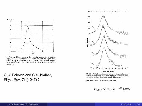
FrG. 8. Cross section for photo-fission of uranium.Because of approximations made in the analysis anduncertainty of the experimental data for low x-ray energies,this curve must be considered of only qualitative sig-nificance.
The determination of the cross section in-volves first drawing a smooth curve through theexperimental points, multiplying the ordinatesof this curve by a function known only roughly, ,
and then differentiating the product; It is evidentthat the given data are not sufficiently preciseto determine the cross section as a function ofenergy, even if the calculation of r(E) wereexact, since in this case the portion of the yieldcurve which is most significant to the deter-mination of the cross section is that below 30Mev. The experimental points in this region aresubject to considerable Huctuation, and the trueyield curve may be appreciably different fromthat shown in Fig. 3. It is also true that theeffects of the approximations made in calculatingr(E) are more serious at low energies. Therefore,it must be stressed that no significance can beattributed to the shape of the curve of 0 vs. 8nor to the absolute values of the cross sectiongiven on the scale of ordinates. The curve of
G.C. Baldwin and G.S. Klaiber,Phys. Rev. 71 (1947) 3
EGDR ∝ 80 · A−1/3 MeV
V.Yu. Ponomarev (TU Darmstadt) 13.05.2014 3 / 31
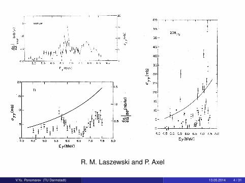
R. M. Laszewski and P. Axel
V.Yu. Ponomarev (TU Darmstadt) 13.05.2014 4 / 31
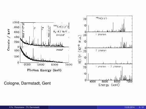
Cologne, Darmstadt, Gent
V.Yu. Ponomarev (TU Darmstadt) 13.05.2014 5 / 31
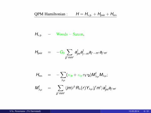
QPM Hamiltonian : H = Hs.p. + Hpair + Hres
Hs.p. − Woods− Saxon,
Hpair = −G0
∑jj′mm′
a†jma†j−maj′−m′aj′m′
Hres = −∑λµ
(κis + κivτ1τ2)M†λµMλµ;
M†λµ =∑
jj′mm′〈jm|iλRλ(r)Yλµ|j ′m′〉a†jmaj′m′
V.Yu. Ponomarev (TU Darmstadt) 13.05.2014 6 / 31
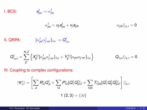
I. BCS: a†jm → α†jm
α†jm = uja†jm + vjajm αjm|〉g.s = 0
II. QRPA: [α†jmα†j′m′ ]λµ → Q†λµ
Q†λµi =
N,Z∑jj′
Xλi
jj′ [α†jmα†j′m′ ]λµ + Yλi
jj′ [αjmαj′m′ ]λµ
Qλµi |〉g.s = 0
III. Coupling to complex configurations:
|ΨνJ 〉 =
[∑Ji
RνJiQ†Ji +
∑12
Pν12[Q†1Q†2]J +
∑123
T ν123[Q†1Q†2Q†3]J
]|〉g.s
1 (2,3) = λi
V.Yu. Ponomarev (TU Darmstadt) 13.05.2014 7 / 31
Q+
Q+Q
+Q+
Q+Q
+ Q
+Q
+Q
+
Q+Q
+
Q+ Q
+Q
+
Q+ Q
+ Q
+
Q+ Q
+ Q
+
Q+Q
+
0
0ν ν
1ν2
ν
νν1
ν2
ν1
ν2
ν3
ν4
ν5
ν1
ν2
ν1
ν2
ν3
ν1
ν2
ν3
ν4
ν5
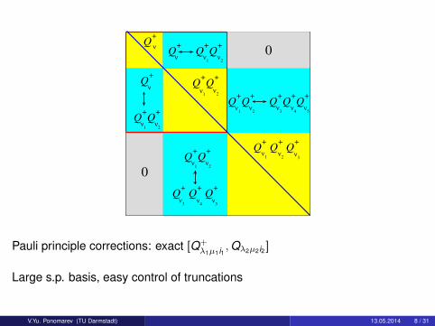
Pauli principle corrections: exact [Q+λ1µ1 i1 ,Qλ2µ2 i2 ]
Large s.p. basis, easy control of truncations
V.Yu. Ponomarev (TU Darmstadt) 13.05.2014 8 / 31
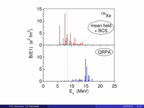
0
5
10
15
0 5 10 15 20 25E
x (MeV)
0
5
10B(E
1)
(e
2 fm
2)
136Xe
mean field+ BCS
QRPA
V.Yu. Ponomarev (TU Darmstadt) 13.05.2014 9 / 31
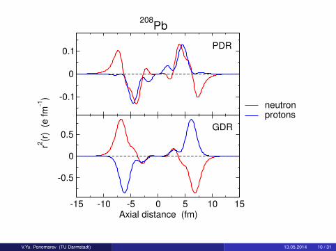
-0.1
0
0.1PDR
neutronprotons
-15 -10 -5 0 5 10 15Axial distance (fm)
-0.5
0
0.5
r2(r
) (
e f
m-1
)
GDR
208Pb
V.Yu. Ponomarev (TU Darmstadt) 13.05.2014 10 / 31
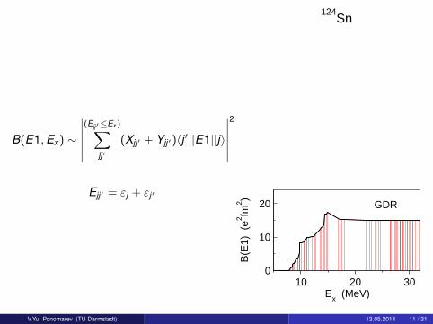
B(E1,Ex ) ∼
∣∣∣∣∣∣(Ejj′≤Ex )∑
jj′(Xjj′ + Yjj′)〈j ′||E1||j〉
∣∣∣∣∣∣2
Ejj′ = εj + εj′
10 20 30Ex (MeV)
0
10
20
B(E
1) (
e2 fm2 )
GDR
PDR
non-collective
124Sn
V.Yu. Ponomarev (TU Darmstadt) 13.05.2014 11 / 31
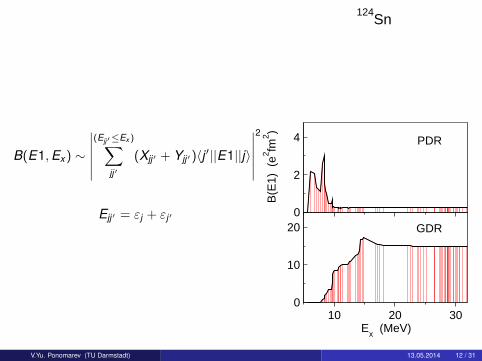
B(E1,Ex ) ∼
∣∣∣∣∣∣(Ejj′≤Ex )∑
jj′(Xjj′ + Yjj′)〈j ′||E1||j〉
∣∣∣∣∣∣2
Ejj′ = εj + εj′ 0
2
4
B(E
1) (
e2 fm2 )
10 20 30Ex (MeV)
0
10
20 GDR
PDR
non-collective
124Sn
V.Yu. Ponomarev (TU Darmstadt) 13.05.2014 12 / 31
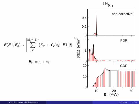
B(E1,Ex ) ∼
∣∣∣∣∣∣(Ejj′≤Ex )∑
jj′(Xjj′ + Yjj′)〈j ′||E1||j〉
∣∣∣∣∣∣2
Ejj′ = εj + εj′
0
0.2
0.4
0
2
4
B(E
1) (
e2 fm2 )
10 20 30Ex (MeV)
0
10
20 GDR
PDR
non-collective
124Sn
V.Yu. Ponomarev (TU Darmstadt) 13.05.2014 13 / 31
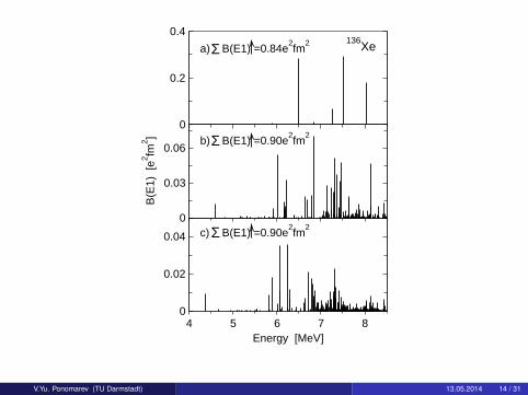
0
0.2
0.4
a)136
XeΣ B(E1) =0.84e2fm
2
0
0.03
0.06B
(E1)
[e2 fm
2 ] b)Σ B(E1) =0.90e2fm
2
4 5 6 7 8Energy [MeV]
0
0.02
0.04 c) B(E1) =0.90e2fm
2Σ
V.Yu. Ponomarev (TU Darmstadt) 13.05.2014 14 / 31
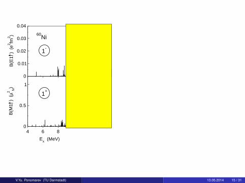
0
0.01
0.02
0.03
0.04
B(E
1 )
(e2 fm
2 )
4 6 8
Ex (MeV)
0
0.5
1
B(M
1 )
(µ2 N
)
60Ni
1-
1+
60Ni 1
-
68Ni
V.Yu. Ponomarev (TU Darmstadt) 13.05.2014 15 / 31
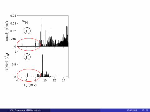
0
0.01
0.02
0.03
0.04
B(E
1 )
(e2 fm
2 )
4 6 8 10 12 14
Ex (MeV)
0
0.5
1
B(M
1 )
(µ2 N
)
60Ni
1-
1+
60Ni 1
-
68Ni
V.Yu. Ponomarev (TU Darmstadt) 13.05.2014 16 / 31
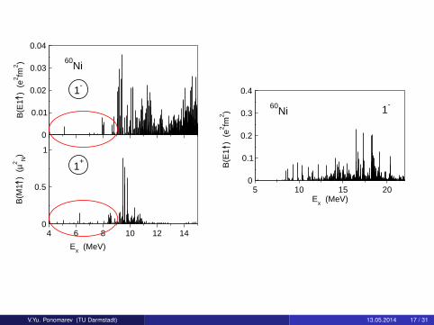
0
0.01
0.02
0.03
0.04
B(E
1 )
(e2 fm
2 )
4 6 8 10 12 14
Ex (MeV)
0
0.5
1
B(M
1 )
(µ2 N
)
60Ni
1-
1+
5 10 15 20Ex (MeV)
0
0.1
0.2
0.3
0.4
B(E
1 )
(e2 fm
2 )
60Ni 1
-
68Ni
V.Yu. Ponomarev (TU Darmstadt) 13.05.2014 17 / 31
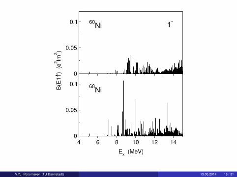
0
0.05
0.1
4 6 8 10 12 14
Ex (MeV)
0
0.05
0.1
B(E
1
) (
e2fm
2)
60Ni 1
-
68Ni
V.Yu. Ponomarev (TU Darmstadt) 13.05.2014 18 / 31
V.Yu. Ponomarev (TU Darmstadt) 13.05.2014 19 / 31
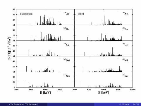
0
20
40
60
Experiment136
Xe
0
20
40
60
138Ba
0
20
40
60
B(E
1)[10-3e2fm
2]
140Ce
0
20
40
60
142Nd
0
20
40
60
2000 4000 6000 8000
E [keV]
144Sm
QPM136
Xe
138Ba
140Ce
142Nd
2000 4000 6000 8000 10000
E [keV]
144Sm
V.Yu. Ponomarev (TU Darmstadt) 13.05.2014 20 / 31
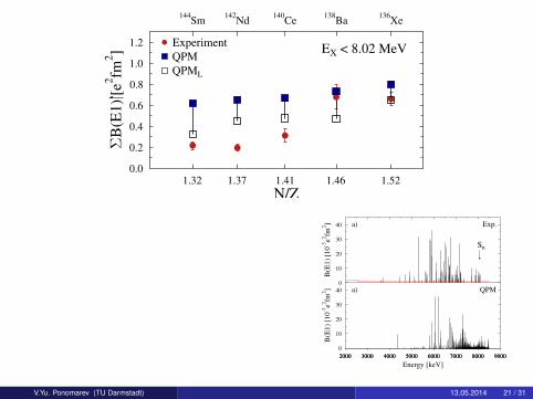
0.0
0.2
0.4
0.6
0.8
1.0
1.2
B(E1)[e
2fm
2]
1.521.461.411.371.32
N/Z
136Xe
138Ba
140Ce
142Nd
144Sm
.....
.Experiment
QPM
QPML
EX < 8.02 MeV
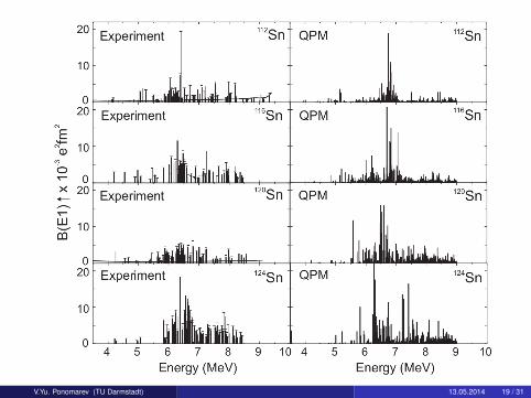
0
10
20
30
40
B(E1)[10-3e2fm
2] Exp.a)
0
10
20
30
40
B(E1)[10-3e2fm
2]
2000 3000 4000 5000 6000 7000 8000 9000
Energy [keV]
2000 3000 4000 5000 6000 7000 8000 9000
QPMa)
Sn
V.Yu. Ponomarev (TU Darmstadt) 13.05.2014 21 / 31
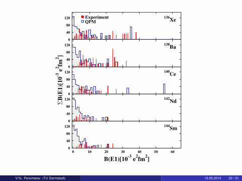
0
40
80
120 136Xe
ExperimentQPM
0
40
80
120 138Ba
0
40
80
120
B(E1)[10-3e2fm
2]
140Ce
0
40
80
120 142Nd
0
40
80
120
0 10 20 30 40 50 60
B(E1)[10-3e2fm
2]
144Sm
V.Yu. Ponomarev (TU Darmstadt) 13.05.2014 22 / 31
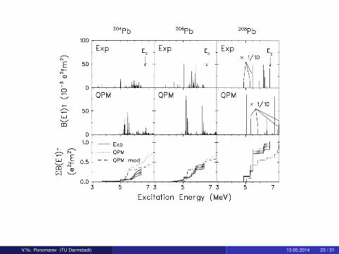
V.Yu. Ponomarev (TU Darmstadt) 13.05.2014 23 / 31
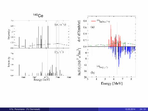
140Ce
V.Yu. Ponomarev (TU Darmstadt) 13.05.2014 24 / 31
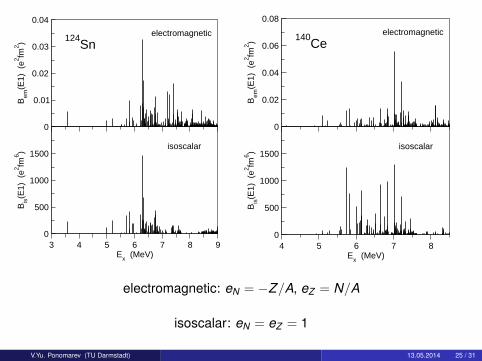
0
0.01
0.02
0.03
0.04B
em(E
1) (
e2 fm2 ) 124
Snelectromagnetic
3 4 5 6 7 8 9Ex (MeV)
0
500
1000
1500
Bis(E
1) (
e2 fm6 )
isoscalar
0
0.02
0.04
0.06
0.08
Bem
(E1)
(e2 fm
2 )4 5 6 7 8
Ex (MeV)
0
500
1000
1500
Bis(E
1) (
e2 fm6 )
140Ce
electromagnetic
isoscalar
electromagnetic: eN = −Z/A, eZ = N/A
isoscalar: eN = eZ = 1
V.Yu. Ponomarev (TU Darmstadt) 13.05.2014 25 / 31
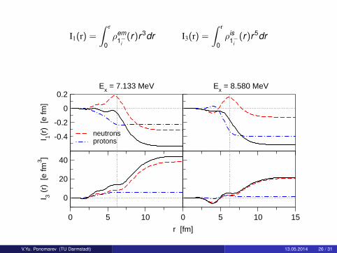
I1(r) =
∫ r
0ρem
1−i(r)r3dr I3(r) =
∫ r
0ρis
1−i(r)r5dr
-0.4
-0.2
0
0.2
I 1(r)
[e fm
]
neutronsprotons
0 5 10
r [fm]
0
20
40
I 3 (r)
[e
fm3 ]
0 5 10 15
Ex = 7.133 MeV Ex = 8.580 MeV
V.Yu. Ponomarev (TU Darmstadt) 13.05.2014 26 / 31
V.Yu. Ponomarev (TU Darmstadt) 13.05.2014 27 / 31
V.Yu. Ponomarev (TU Darmstadt) 13.05.2014 28 / 31
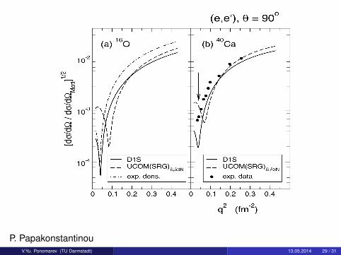
P. PapakonstantinouV.Yu. Ponomarev (TU Darmstadt) 13.05.2014 29 / 31
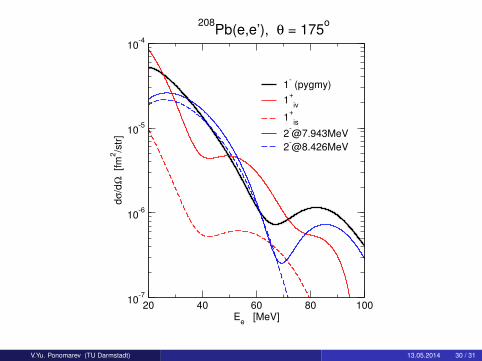
20 40 60 80 100E
e [MeV]
10-7
10-6
10-5
10-4
dσ
/dΩ
[fm
2/s
tr]
1- (pygmy)
1+
iv
1+
is
208Pb(e,e’), θ = 175
o
V.Yu. Ponomarev (TU Darmstadt) 13.05.2014 30 / 31
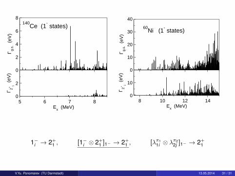
0
2
4
6
8
Γ g.s. (
eV)
5 6 7 8Ex (MeV)
0
2
Γ 2+1 (
eV)
140Ce (1
- states)
0
10
20
30
40
Γ g.s. (
eV)
8 10 12 14Ex (MeV)
0
10
Γ 2+1 (
eV)
60Ni (1
- states)
1−i → 2+1 , [1−i ⊗ 2+
1 ]1− → 2+1 , [λπ1
1i ⊗ λπ22j ]1− → 2+
1
V.Yu. Ponomarev (TU Darmstadt) 13.05.2014 31 / 31