Lecture Notes on Function Spaces · space invaders Karoline Götze TU Darmstadt, WS 2010/2011....
82
Transcript of Lecture Notes on Function Spaces · space invaders Karoline Götze TU Darmstadt, WS 2010/2011....
Lecture Notes on Function Spaces
space invaders
Karoline Götze
TU Darmstadt, WS 2010/2011
Contents
1 Basic Notions in Interpolation Theory 5
2 The K-Method 15
3 The Trace Method 19
3.1 Weighted Lp spaces . . . . . . . . . . . . . . . . . . . . . . . . . . . . . . . 193.2 The spaces V (p, θ,X0, X1) . . . . . . . . . . . . . . . . . . . . . . . . . . . 203.3 Real interpolation by the trace method and equivalence . . . . . . . . . . 21
4 The Reiteration Theorem 26
5 Complex Interpolation 31
5.1 X-valued holomorphic functions . . . . . . . . . . . . . . . . . . . . . . . . 325.2 The spaces [X,Y ]θ and basic properties . . . . . . . . . . . . . . . . . . . 335.3 The complex interpolation functor . . . . . . . . . . . . . . . . . . . . . . 365.4 The space [X,Y ]θ is of class Jθ and of class Kθ. . . . . . . . . . . . . . . . 37
6 Examples 41
6.1 Complex interpolation of Lp -spaces . . . . . . . . . . . . . . . . . . . . . 416.2 Real interpolation of Lp-spaces . . . . . . . . . . . . . . . . . . . . . . . . 43
6.2.1 Lorentz spaces . . . . . . . . . . . . . . . . . . . . . . . . . . . . . 436.2.2 Lorentz spaces and the K-functional . . . . . . . . . . . . . . . . . 456.2.3 The Marcinkiewicz Theorem . . . . . . . . . . . . . . . . . . . . . . 48
6.3 Hölder spaces . . . . . . . . . . . . . . . . . . . . . . . . . . . . . . . . . . 496.4 Slobodeckii spaces . . . . . . . . . . . . . . . . . . . . . . . . . . . . . . . 516.5 Functions on domains . . . . . . . . . . . . . . . . . . . . . . . . . . . . . 54
7 Function Spaces from Fourier Analysis 56
8 A Trace Theorem 68
9 More Spaces 76
9.1 Quasi-norms . . . . . . . . . . . . . . . . . . . . . . . . . . . . . . . . . . . 769.2 Semi-norms and Homogeneous Spaces . . . . . . . . . . . . . . . . . . . . 769.3 Orlicz Spaces LA . . . . . . . . . . . . . . . . . . . . . . . . . . . . . . . . 789.4 Hardy Spaces . . . . . . . . . . . . . . . . . . . . . . . . . . . . . . . . . . 809.5 The Space BMO . . . . . . . . . . . . . . . . . . . . . . . . . . . . . . . . 81
2
Motivation
Examples of function spaces:
C(Rn; R), C1([−1, 1]), Cα(Ω; C), Lp(X, ν), W k,p(Ω), W s,p, Bsp,q,
where Ω domain in Rn, α ∈ R+, 1 ≤ p, q ≤ ∞, (X, ν) measure space, k ∈ N, s ∈ R+.
Philosophy: Objectify function spaces
Example: We can consider H1/2 as
• interpolation space: L2 ∩H1 → H1/2 → L2 +H1, H1/2 = F(L2,H1)
• embedded space: H1 ⊂ H1/2 ⊂ L2
• space of functions f ∈ L2 with one half of a derivative: |ξ|1/2f ∈ L2
• trace space: γ : H1(Rn+) → H1/2(Rn−1) is bounded and surjective.
3

Books
Author: Title, ReferenceWhich topics in the lecture?Comment
Where in the Notes?
Adams/Fournier SobolevSpaces, [1]
Sobolev Spaces, Orlicz SpacesFunctions on Domains
Sections 6.5, 9.3
Bennett/Sharpley:Interpolation of Operators, [2]
very nice elaborate proofs Sections 6.2, 9.4, 9.5
Bergh/Löfström:Interpolation Spaces, [3]
often short proofs,nice structure for us
Chapters 7, 8Section 9.2
Lunardi: InterpolationTheory, [5]
very good introduction,very nice proofs
Chapters 2,3,4,5
Lunardi: Analytic Semigroups
and Optimal Regularity of
Parabolic Problems, [4]
book on a dierent topic,for us: Hölder spaces
Section 6.3
Tartar: An Introduction to
Sobolev Spaces and
Interpolation Spaces, [6]
nd history, references andideas
inbetween
Triebel: Interpolation Theory,
Function Spaces, Dierential
Operators, [7]
nd everything, dicult forproofs
Chapter 1, everywhereinbetween
4
1 Basic Notions in Interpolation Theory
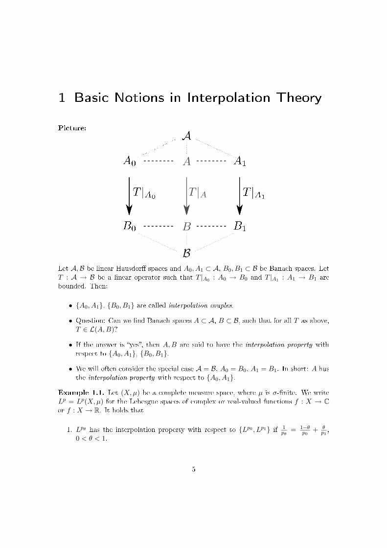
Picture:
Let A,B be linear Hausdor spaces and A0, A1 ⊂ A, B0, B1 ⊂ B be Banach spaces. LetT : A → B be a linear operator such that T |A0 : A0 → B0 and T |A1 : A1 → B1 arebounded. Then:
• A0, A1, B0, B1 are called interpolation couples.
• Question: Can we nd Banach spaces A ⊂ A, B ⊂ B, such that for all T as above,T ∈ L(A,B)?
• If the answer is yes, then A,B are said to have the interpolation property withrespect to A0, A1, B0, B1.
• We will often consider the special case A = B, A0 = B0, A1 = B1. In short: A hasthe interpolation property with respect to A0, A1.
Example 1.1. Let (X,µ) be a complete measure space, where µ is σ-nite. We writeLp = Lp(X,µ) for the Lebesgue spaces of complex or real-valued functions f : X → Cor f : X → R. It holds that
1. Lpθ has the interpolation property with respect to Lp0 , Lp1 if 1pθ
= 1−θp0
+ θp1,
0 < θ < 1.
5
1 Basic Notions in Interpolation Theory
2. The space C1([−1, 1]) (= C1([−1, 1]; R)) does not have the interpolation propertywith respect to C([−1, 1]), C2([−1, 1]).
Theorem 1.2. (Convexity Theorem of Riesz/Thorin)Let 1 ≤ p0, p1, q0, q1 ≤ ∞, p0 6= p1, q0 6= q1 and T a linear operator such that T :Lpi(X,µ) → Lqi(Y, ν), i ∈ (0, 1) is bounded linear. Then for every 0 < θ < 1,
T : Lpθ(X,µ) → Lqθ(Y, ν) is linear and bounded,
for 1pθ
= 1−θp0
+ θp1, 1qθ
= 1−θq0
+ θq1. Furthermore, the estimate
‖T‖L(Lpθ ,Lqθ ) ≤ C‖T‖1−θL(Lp0 ,Lq0 )‖T‖
θL(Lp1 ,Lq1 )
holds true.
Remark 1.3. About the above theorem:
• If the Lp are complex-valued, C = 1. If they are real-valued, C = 2.
• Example 1 immediately follows from Theorem 1.2.
• Riesz 1926, Thorin 1939/48: Interpolation result which existed before interpolationtheory. The direct proof contains ideas for general constructions of interpolationspaces (As and Bs in the picture). For us, this means that the proof will be givenin a later Chapter :-).
• Why convexity: The theorem shows that the function f given by f(1p ,
1q ) =
‖T‖L(Lp,Lq) is logarithmically convex, i.e.
f
((1− θ)(
1p0,
1q0
) + θ(1p1,
1q1
))≤ f(
1p0,
1q0
)1−θf(1p1,
1q1
)θ
or, in other words, g = log f is convex.
Reminder: f ∈ Ck([−1, 1]) ⇔ f : [−1, 1] → R is k-times continuously dierentiable and‖f‖Ck([−1,1]) :=
∑kl=0
1l! supx∈[−1,1] |f (k)(x)| <∞ (we can replace sup by max).
Theorem 1.4. (Mitjagin/Semenov '76)For every ε ∈ (0, 1] let Vε : C([−1, 1]) → C([−1, 1]) be given by
(Vεf)(x) := 1
−1
x
x2 + y2 + ε2(f(y)− f(0)) dy. (1.1)
Then for all ε ∈ (0, 1], it holds that
1. Vε ∈ C∞([−1, 1]),
2. ‖Vε‖L(C([−1,1])) < 2π,
6
1 Basic Notions in Interpolation Theory
3. ‖Vε‖L(C2([−1,1])) < 5π + 2,
4. given fε(y) =√y2 + ε2 − ε, we get ‖fε‖C1([−1,1]) ≤ 2, but (Vεfε)′(0) > 2 ln( 1
5ε).
Corollary 1.5. From Theorem 1.4 we get Example 2.
Proof. The proof of the corollary will be given as an exercise. Proof of Theorem 1.4:
In the following, we write Ck for Ck([−1, 1]) and C0 for C([−1, 1])
1. Dierentiation in the integral in (1.1).
2. Calculate:
|Vεf(x)| ≤ 1
−1
|x|x2 + y2 + ε2
2‖f‖C0 dy
≤symmetry
4‖f‖C0 |x| 1
0
1x2 + y2
dy
≤ 4‖f‖C0 |x|[1|x|
arctan(y
|x|)]10
≤ 2π‖f‖C0 .
3. Identity map: h(y) = y, then
(Vεh)(x) = 1
−1
xy
x2 + y2 + ε2dy = 0 (1.2)
for all x ∈ [−1, 1]. Taylor Theorem: If f ∈ C2, then
f(y) = f(0) + f ′(0)y + r2(f, y) (1.3)
for some r2(f, ·) ∈ C0 and
|r2(f, y)| =|f ′′(ϑy)|
2y2 ≤ ‖f‖C2y2. (1.4)
It follows from (1.2) and (1.3) that
(Vεf)(s) = 1
−1
x
x2 + y2 + ε2[f(y)− f(0)− f ′(0)y] dy
= 1
−1
x
x2 + y2 + ε2r2(f, y) dy.
Note that
| ddx
(x
x2 + y2 + ε2)| = | y2 + ε2 − x2
(x2 + y2 + ε2)2| < 1
x2 + y2 + ε2<
1y2 + ε2
7
1 Basic Notions in Interpolation Theory
and
| d2
dx2(
x
x2 + y2 + ε2)| = 2|x||x2 − 3y2 − 3ε2|
(x2 + y2 + ε2)3<
6|x|(x2 + y2 + ε2)2
.
In conclusion, from (1.4), we get
|(Vεf)′(x))| ≤ 1
−1
∣∣∣∣ ddx(x
x2 + y2 + ε2)∣∣∣∣ |r2(f, y)| dy
≤ ‖f‖C2
1
−1
y2
y2 + ε2dy ≤ 2‖f‖C2
and
|(Vεf)′′(x))| ≤ 1
−1
6|x|(x2 + y2 + ε2)2
‖f‖C2y2 dy
≤ 12‖f‖C2
1
0
|x|x2 + y2
dy ≤ 6π‖f‖C2 ,
so ‖Vεf‖C2 ≤ (2π + 2 + 3π)‖f‖C2 for all f ∈ C2.
4. We see: The fε approximate | · |. Note that
f ′′ε (0) =ε2
(y2 + ε2)3/2|y=0 =
1ε
ε→0−→∞
(i.e. Vε : C2 → C2 is ok!). Moreover, |fε(y)| = y2√y2+ε2+ε
< |y| ≤ 1 and |f ′ε(y)| =|y|√y2+ε2
< 1. The interesting part is:
(Vεfε)′(x) = 1
−1
y2 + ε2 − x2
(x2 + y2 + ε2)2(√y2 + ε2 − ε) dy
x=0= 1
−1
√y2 + ε2 − ε
y2 + ε2dy
u= yε= 2
1/ε
0
√u2 + 1− 1u2 + 1
du
= 2 1/ε
0
1√u2 + 1
du− 2 1/ε
0
1u2 + 1
du
≥ 2 1/ε
0
1u+ 1
du− 2 arctan(1ε)
≥ 2 ln(1 +1ε)− π > 2 ln(
1 + 1ε
eπ/2) > 2 ln(
15ε
).
8
1 Basic Notions in Interpolation Theory
Notation: We write A → B i id : A→ B is bounded.
Lemma 1.6. Let A0, A1 be an interpolation couple. Then
A0 +A1 = a ∈ A : ∃a0 ∈ A0,∃a1 ∈ A1, a = a0 + a1
with the norm
‖a‖A0+A1 = infa=a0+a1,ai∈Ai
(‖a0‖A0 + ‖a1‖A1)
and
A0 ∩A1 = a ∈ A : a ∈ A0, a ∈ A1
with the norm
‖a‖A0∩A1 = max(‖a‖A0 , ‖a‖A1)
are Banach spaces. It holds that
A0 ∩A1 → Ai → A0 +A1.
Proof. Exercise.
Denition 1.7. (Basic denitions in category theory)
1. A category consists of
a) a class of objects A,B,C, . . . and
b) a class of pairwise disjoint non-empty sets [A,B]. Each ordered pair (A,B)uniquely corresponds to a set [A,B]. The elements in [A,B] are called mor-
phisms.
2. For every ordered triplet (A,B,C) of objects, we have the composition of mor-phisms via
V : [B,C]× [A,B] → [A,C].
Notation: f ∈ [A,B], g ∈ [B,C], then gf = V (g, f). Moreover, we have associa-tivity
f ∈ [A,B], g ∈ [B,C], h ∈ [C,D], then (hg)f = h(gf)
and for all objects A, there exists an identity idA ∈ [A,A], such that for all f ∈[B,A], g ∈ [A,B],
idAf = f and gidA = g.
3. Let C1, C2 be two categories. A map F : C1 → C2 is called a (covariant) functor, if
a) for all objects A in C2, F(A) is an object in C1,
9
1 Basic Notions in Interpolation Theory
b) for all morphisms f ∈ [A,B] in C2, F(f) ∈ [F(A),F(B)] is a morphism in C1,
c) F(idA) = idF(A) for all objects A in C2,
d) F(gf) = F(g)F(f) for all morphisms f ∈ [A,B], g ∈ [B,C].
Example 1.8. The notions categories are strong in some areas of mathematics, likegeometry. For more examples, check e.g. Wikipedia :). For us, the following are relevant,
• Category C1: (complex) Banach spaces A,B,C, . . . are objects, bounded linearoperators T ∈ [A,B] = L(A,B) are morphisms.
• Category C2: interpolation couples A0, A1, B0, B1, . . . are objects and
[A0, A1, B0, B1] = L(A0, A1, B0, B1)
are sets of morphisms, where T : A0 + A1 → B0 + B1, T ∈ L(A0, A1, B0, B1)if T |A0 : A0 → B0, T |A1 : A1 → B1 are bounded.
Remark 1.9. The space L(A0, A1, B0, B1) is a Banach space with the norm
‖T‖L(A0,A1,B0,B1) = max(‖T |A0‖L(A0,B0), ‖T |A1‖L(A1,B1))
andL(A0, A1, B0, B1) → L(A0 +A1, B0 +B1). (1.5)
Proof. Let
D = (U, V ) : U ∈ L(A0, B0), V ∈ L(A1, B1), U = V on A0 ∩A1⊂ L(A0, B0)× L(A1, B1),
where
‖(U, V )‖D = ‖(U, V )‖L(A0,B0)×L(A1,B1) = max(‖U‖L(A0,B0), ‖V ‖L(A1,B1)).
We show that
1. D is a closed subspace of L(A0, B0)× L(A1, B1), i.e. it is a Banach space,
2. D is isometrically isomorphic to L(A0, A1, B0, B1).
Regarding 1.: Let (Un, Vn) → (U, V ) ∈ L(A0, A1, B0, B1) for some (Un, Vn)n ⊂ D,so
max(‖U − Un‖L(A0,B0), ‖V − Vn‖L(A1,B1)) → 0.
We have to show that U = V on A0 ∩A1. For every a ∈ A0 ∩A1,
Ua− V a = (U − Un)a+ (Un − Vn)a+ (Vn − V )a
10
1 Basic Notions in Interpolation Theory
where Un − Vn ≡ 0, (U − Un)a → 0 in B0 and (Vn − V )a → 0 in B1. By embedding,(U − Un)a+ (Vn − V )a→ 0 in B0 +B1, so U = V on A0 ∩A1.Regarding 2.: We consider j : L(A0, A1, A1, B1) → D, given by j(T ) = (T |A0 , T |A1).It follows that j is linear and isometric, therefore injective. It remains to show that j issurjective. Let (U , V ) ∈ D. We dene T : A0 +A1 → B0 +B1 by
T a = T (a0 + a1) = Ua0 + Ua1.
T is well-dened: Let a0 + a1 = a = a′0 + a′1, then a′0 − a0 = a1 − a′1 ∈ A0 ∩A1, so
T (a0 + a1) = Ua0 + V a1 = U(a0 − a′0) + Ua′0 + V a′1 − V (a′1 − a1) = T (a′0 + a′1)
since U = V on A0 ∩ A1. It is clear that T ∈ L(A0, A1, B0, B1) and j(T ) = (U , V ).It remains to show (1.5). For all a = a0 + a1, a0 ∈ A0, a1 ∈ A1, we have
‖Ta‖B0+B1 = infTa=b0+b1,bi∈Bi
(‖b0‖B0 + ‖b1‖B1)
≤ ‖Ta0‖B0 + ‖Ta1‖B1
≤ max(‖T |A0‖L(A0,B0), ‖T |A1‖L(A1,B1)
)(‖a0‖A0 + ‖a1‖A1).
We take the inmum over a = a0 + a1 to get that
‖Ta‖B0+B1 ≤ ‖T‖L(A0,A1,B0,B1)‖a‖A0+A1 .
We are now in a position to give a formulation of interpolation of Banach spaces in thelanguage of categories.
Denition 1.10. A functor F : C2 → C1 is called interpolation functor, if for everyA0, A1, B0, B1 in C2,
A0 ∩A1 → F(A0, A1) → A0 +A1
andT ∈ L(A0, A1, B0, B1) ⇒ F(T ) = T |F(A0,A1).
If F is an interpolation functor, then the space F(A0, A1) is called interpolation space
with respect to A0, A1.
Note that this denition ts the picture at the beginning of the chapter, as if F(A0, A1)is an interpolation space in the sense of the denition, it also has the interpolation prop-erty with respect to A0, A1. It is interesting that also something like the opposite holdstrue. If A0, A1 is an interpolation couple and there is a Banach spaces A such thatA0∩A1 → A → A0 +A1 and such that Im(T |A) ⊂ A for all T ∈ L(A0, A1, A0, A1)),then there exists an interpolation functor F0 such that A = F(A0, A1). The proof ofthis fact is an exercise, given Theorem 1.14 at the end of this chapter.
11
1 Basic Notions in Interpolation Theory
Denition 1.11. An interpolation functor F is called of type θ, 0 < θ < 1, if thereexists a constant C > 0, such that for all A0, A1, B0, B1,T in C2,
‖T‖L(F(A0,A1,FB0,B1) ≤ C‖T‖1−θL(A0,B0)‖T‖
θL(A1,B1).
If we can choose C = 1, F is called exact. Note: It is always true that C ≥ 1.
Even if we do not know whether a functor is of type θ or exact, the following theoremshows that we always have some estimate of this type, uniformly in T , but depending onthe interpolation space.
Theorem 1.12. Let F be an interpolation functor, A0, A1, B0, B1 interpolation
couples and A = F(A0, A1), B = F(B0, B1) interpolation spaces. Then there exists
a constant C(A,B) > 0 such that
‖T‖L(A,B) ≤ C(A,B) max(‖T‖L(A0,B0), ‖T‖L(A1,B1)
)for all T ∈ L(A0, A1, B0, B1).
In order to prove this theorem, we need the following lemma, whose proof is left as anexercise.
Lemma 1.13. Let U, V,X, Y be Banach spaces such that U → X, V → Y and S : U →V such that S ∈ L(X,Y ). Then we also get S ∈ L(U, V ).
Proof. of Theorem 1.12. We use Lemma 1.13 with U = L(A0, A1, B0, B1), V =L(A,B), X = L(A0 +A1, B0 +B1), Y = L(A,B0 +B1) and S : L(A0 +A1, B0 +B1) →L(A,B0 + B1) given by S(T ) = T |A. In view of (1.5), we only need to verify thatV → Y and that S is bounded. The rst can be derived directly from the embeddingB → B0 + B1. the boundedness of S follows from the embedding A → A0 + A1. Moreprecisely, for all a ∈ A,
‖Ta‖B0+B1 ≤ ‖T‖L(A0+A1,B0+B1)‖a‖A0+A1
≤ C(A)‖T‖L(A0+A1,B0+B1)‖a‖A,
so ‖ST‖L(A,B0+B1) ≤ C(A)‖T‖L(A0+A1,B0+B1). Clearly, the constants involved do notdepend on T .
As a closing to this abstract chapter, we look at the following theorem, justiying theuse of interpolation functors for interpolation theory.
Theorem 1.14. (Aronszajn/Gagliardo '65)Let C1,C2 be as in Example 1.8, let A0, A1 be an interpolation couple and let A be such
that
A0 ∩A1 → A → A0 +A1
and T (A) ⊂ A for all T ∈ L(A0, A1). Then there exists an interpolation functor
F0 : C2 → C1 such that F0(A0, A1) = A.
12
1 Basic Notions in Interpolation Theory
Proof. We give a proof in seven small steps.
1. Preliminary observation: By Lemma 1.13, T (A) ⊂ A implies that T ∈ L(A).
2. Construction of F0: Let X0, X1 be an object in C2. We dene
X = F0(X0, X1) = x ∈ X0 +X1 : x =∞∑j=1
Tjaj abs. conv. ,
aj ∈ A, Tj ∈ L(A0, A1, X0, X1), j ∈ N,where
‖x‖X = infx=
P∞j=1 Tjaj
∞∑j=1
‖Tj‖L(A0,A1,X0,X1)‖aj‖A <∞.
It follows that ‖ · ‖X is a norm for X.
3. Show X0 ∩X1 → X: Let ϕ : A0 + A1 → C a bounded linear functional such thatϕ(a∗) = 1 for some a∗ ∈ A. Dene ‖ϕ‖ = c∗. For every x ∈ X0 ∩X1, we dene
Tx : A0 +A1 → X0 +X1, Txa := ϕ(a)x.
It follows that for i ∈ 0, 1 and a ∈ Ai,
‖Txa‖Xi = |ϕ(a)|‖x‖Xi ≤ c∗‖a‖A0+A1‖x‖Xi ≤ c‖a‖Ai‖x‖Xi ,
so Tx ∈ L(A0, A1, X0, X1) and
‖Tx‖L(A0,A1,X0,X1) ≤ cmaxi
(‖Tx‖L(Ai,Xi)) ≤ cmaxi‖x‖Xi = c‖x‖X0∩X1 .
Now for every x ∈ X0 ∩X1, x = Txa∗ ∈ X and
‖x‖X ≤ ‖Tx‖L(A0,A1,X0,X1)‖a∗‖A ≤ c‖a∗‖A‖x‖X0∩X1 .
4. Show that X → X0 +X1: Let x =∑∞
j=1 Tjaj ∈ X. Then by Remark 1.9,
‖x‖X0+X1 ≤∞∑j=1
‖Tjaj‖X0+X1
≤∞∑j=1
‖Tj‖L(A0+A1,X0+X1)‖aj‖A0+A1
≤ c
∞∑j=1
‖Tj‖L(A0,A1,X0,X1)‖aj‖A.
Taking the inf, we get ‖x‖X0+X1 ≤ c‖x‖X .
13
1 Basic Notions in Interpolation Theory
5. X is complete: If for some (xn)n ⊂ X,∑∞
n=1 ‖xn‖X < ∞ then by Step 4,∑∞n=1 ‖xn‖X0+X1 <∞, so that the limit
∑∞n=1 xn = x exists in X0+X1. Moreover,
by denition, for all n ∈ N, there exist Tnj ∈ L(A0, A1, X0, X1), anj ∈ A, suchthat xn =
∑∞j=1 T
nj a
nj and
∞∑j=1
‖Tnj ‖L(A0,A1,X0,X1)‖anj ‖A < ‖xn‖X + 2−n,
so x =∑∞
n=1
∑∞j=1 T
nj a
nj . Taking the inf, we get ‖x‖X <
∑∞n=1 ‖xn‖X + 1. It
follows that∑m
n=1 xnm→∞→ x in X.
6. F0 on morphisms in C2: Let X0, X1, Y0, Y1 be objects in C2, and let S ∈L(X0, X1, Y0, Y1) be a morphism. We setX = F0(X0, X1), Y = F0(Y0, Y1)and F0(S) := S|X . We need to show that F0(S) ∈ L(X,Y ). Let x =
∑∞j=1 Tjaj ,
where Tj ∈ L(A0, A1, X0, X1), aj ∈ A. Then Sx =∑∞
j=1 STjaj , whereSTj ∈ L(A0, A1, Y0, Y1). It follows that for every suitable choice of Tj , aj ,
‖Sx‖Y ≤∞∑j=1
‖STj‖L(A0,A1,Y0,Y1)‖aj‖A
≤ ‖S‖L(X0,X1,Y0,Y1)
∞∑j=1
‖Tj‖L(A0,A1,X0,X1)‖aj‖A.
Taking the inf, we get ‖Sx‖Y ≤ ‖S‖L(X0,X1,Y0,Y1)‖x‖X .
7. We show that F0(A0, A1) = A: It is clear that A ⊂ F0(A0, A1). For theopposite inclusion, let a =
∑∞j=1 Tjaj be in F0(A0, A1) as above. By Theorem
1.12, there exists a constant c(A), such that for all j ∈ N,
‖a‖A ≤∞∑j=1
‖Tjaj‖A ≤ c(A)∞∑j=1
‖Tj‖L(A0,A1)‖aj‖A.
Taking the inmum, we get ‖a‖A ≤ c(A)‖a‖F0(A0,A1).
14
2 The K-Method
Denition 2.1. Let A0, A1 an interpolation couple. Then (Peetre's) K-functional
K : R+ ×A0 +A1 → R
is dened asK(t, a;A0, A1) = inf
a=a0+a1,ai∈Ai
(‖a0‖A0 + t‖a1‖A1).
Notation: K(t, a) instead of K(t, a;A0, A1).
Lemma 2.2. Fix a ∈ A0 +A1. Then K(·, a) is positive, monotonely increasing, concave
and continuous. It holds that
min(1, t)‖a‖A0+A1 ≤ K(t, a) ≤ max(1, t)‖a‖A0+A1 . (2.1)
Proof. We see immediately: Positivity, monotonicity and (2.1). It remains to show thatK is concave in t, i.e. for all 0 < λ < 1,
K ((1− λ)t1 + λt2, a) ≥ (1− λ)K(t1, a) + λK(t2, a).
Let 0 < t1 < t < t2 < ∞ and λ = t−t1t2−t1 , so that 1 − λ = t2−t
t2−t1 and t = (1 − λ)t1 + λt2.For every a0 ∈ A0, a1 ∈ A1 such that a0 + a1 = a, we have
t2 − t
t2 − t1(‖a0‖A0 + t1‖a1‖A1) +
t− t1t2 − t1
(‖a0‖A0 + t2‖a1‖A1) = ‖a0‖A0 + t‖a1‖A1 .
We rst take the inf on the left hand side to get
t2 − t
t2 − t1K(t1, a) +
t− t1t2 − t1
K(t2, a) ≤ ‖a0‖A0 + t‖a1‖A1 .
Now taking the inf on the right hand side gives
t2 − t
t2 − t1K(t1, a) +
t− t1t2 − t1
K(t2, a) ≤ K(t, a).
Since K(·, a) is concave and monotonely increasing, it is continuous.
Denition 2.3. Let X0, X1 an interpolation couple, 0 < θ < 1 and 1 ≤ q ≤ ∞. Thenwe dene
(X0, X1)θ,q := x ∈ X0 +X1 : ‖x‖(X0,X1)θ,q<∞,
where
‖x‖(X0,X1)θ,q=
(∞0 [t−θK(t, x)]q dt
t
) 1q , q <∞,
sup0<t<∞ t−θK(t, x), q = ∞.
15
2 The K-Method
Theorem 2.4. Let X0, X1 an interpolation couple, 0 < θ < 1 and 1 ≤ q ≤ ∞. Then
1. the space (X0, X1)θ,q is an interpolation space with respect to X0, X1, i.e. there
exists an interpolation functorKθ,q : C2 → C1 such thatKθ,q(X0, X1) = (X0, X1)θ,q.The functor Kθ,q is exact and of type θ.
2. For all x ∈ (X0, X1)θ,q,
K(t, x) ≤ cθ,qtθ‖x‖(X0,X1)θ,q
. (2.2)
Proof. In the following, let X = (X0, X1)θ,q. We rst show (2.2). The case q = ∞ followsimmediately. Otherwise, we rst write s−θq = θq
∞s t−θq dt
t . It follows that
s−θK(s, x) = (θq)1qK(s, x)
( ∞
st−θq
dtt
) 1q
≤ (θq)1q
( ∞
st−θqK(t, x)q
dtt
) 1q
≤ (θq)1q ‖x‖X.
Next, we show 1. in four steps.
1. ‖ · ‖X is a norm:
• ‖x‖X = 0 ⇒ K(t, x) ≡ 0(2.1)⇒ x = 0,
• K(·, λx) = |λ|K(·, x) ⇒ ‖λx‖X = |λ|‖x‖X ,
• K(t, x0 + x1) ≤ K(t, x1) +K(t, x2)Minkowski⇒ ‖x0 + x1‖X ≤ ‖x0‖X + ‖x1‖X .
2. X is complete: Let (xn)n be a Cauchy sequence in X. By (2.2) and since K(1, ·) =‖ · ‖X0+X1 , (xn)n has a limit x in X0 +X1. Assume now q < ∞, analogous proofworks otherwise. For every ε > 0, let n0(ε) be such that ‖xm − xn‖ < ε
2 for everym > n > n0(ε). Moreover, let L > l > 0. Then by monotonicity of K and (2.1),there is m0(ε, θ, l, L), such that for all m ≥ m0(ε, θ, l, L), m > n,
( L
l[t−θK(t, x− xn)]q
dtt
) 1q
≤ ε
2+( L
l[t−θK(t, x− xm)]q
dtt
) 1q
≤ ε
2+ L‖x− xm‖X0+X1
( L
lt−θq
dtt
) 1q
≤ ε
2+ L(
1θq
)1q l−θ‖x− xm‖X0+X1 < ε.
Passing to the limit L→∞, l→ 0 yields the claim.
16
2 The K-Method
3. Show that X0 ∩ X1 → X → X0 + X1: Let x ∈ X0 ∩ X1, then K(t, x) ≤min(1, t)‖x‖X0∩X1 . W.l.o.g., let q <∞. Then
‖x‖qX = 1
0[t−θK(t, x)]q
dtt
+ ∞
1[t−θK(t, x)]q
dtt
≤ ‖x‖X0∩X1( 1
0t(1−θ)q
dtt
+ ∞
1t−θq
dtt
)
≤ Cθ,q‖x‖X0∩X1 .
Clearly, ‖x‖X0+X1 = K(1, x)(2.2)
≤ cθ,q‖x‖X .
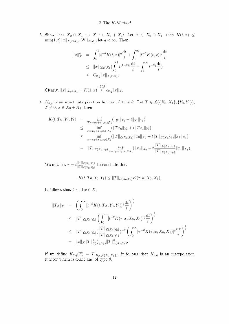
4. Kθ,q is an exact interpolation functor of type θ: Let T ∈ L(X0, X1, Y0, Y1),T 6= 0, x ∈ X0 +X1, then
K(t, Ta;Y0, Y1) = infTx=y0+y1,yi∈Yi
(‖y0‖Y0 + t‖y1‖Y1)
≤ infx=x0+x1,xi∈Xi
(‖Tx0‖Y0 + t‖Tx1‖Y1)
≤ infx=x0+x1,xi∈Xi
(‖T‖L(X0,Y0)‖x0‖X0 + t‖T‖L(X1,Y1)‖x1‖X1)
= ‖T‖L(X0,Y0) infx=x0+x1,xi∈Xi
(‖x0‖X0 + t‖T‖L(X1,Y1)
‖T‖L(X0,Y0)‖x1‖X1).
We now set τ = t‖T‖L(X1,Y1)
‖T‖L(X0,Y0)to conclude that
K(t, Ta;Y0, Y1) ≤ ‖T‖L(X0,Y0)K(τ, a;X0, X1).
It follows that for all x ∈ X,
‖Tx‖Y =( ∞
0[t−θK(t, Tx;Y0, Y1)]q
dtt
) 1q
≤ ‖T‖L(X0,Y0)
( ∞
0[t−θK(τ, x;X0, X1)]q
dtt
) 1q
≤ ‖T‖L(X0,Y0)(‖T‖L(X0,Y0)
‖T‖L(X1,Y1))−θ
( ∞
0[τ−θK(τ, x;X0, X1)]q
dττ
) 1q
= ‖x‖X‖T‖1−θL(X0,Y0)‖T‖
θL(X1,Y1).
If we dene Kθ,q(T ) = T |Kθ,q(X0,X1), it follows that Kθ,q is an interpolationfunctor which is exact and of type θ.
17
2 The K-Method
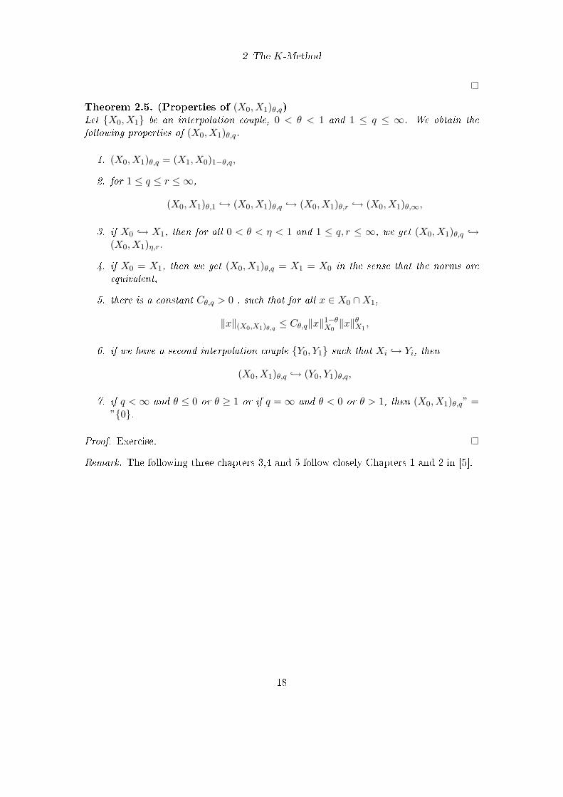
Theorem 2.5. (Properties of (X0, X1)θ,q)Let X0, X1 be an interpolation couple, 0 < θ < 1 and 1 ≤ q ≤ ∞. We obtain the
following properties of (X0, X1)θ,q.
1. (X0, X1)θ,q = (X1, X0)1−θ,q,
2. for 1 ≤ q ≤ r ≤ ∞,
(X0, X1)θ,1 → (X0, X1)θ,q → (X0, X1)θ,r → (X0, X1)θ,∞,
3. if X0 → X1, then for all 0 < θ < η < 1 and 1 ≤ q, r ≤ ∞, we get (X0, X1)θ,q →(X0, X1)η,r.
4. if X0 = X1, then we get (X0, X1)θ,q = X1 = X0 in the sense that the norms are
equivalent,
5. there is a constant Cθ,q > 0 , such that for all x ∈ X0 ∩X1,
‖x‖(X0,X1)θ,q≤ Cθ,q‖x‖1−θ
X0‖x‖θX1
,
6. if we have a second interpolation couple Y0, Y1 such that Xi → Yi, then
(X0, X1)θ,q → (Y0, Y1)θ,q,
7. if q <∞ and θ ≤ 0 or θ ≥ 1 or if q = ∞ and θ < 0 or θ > 1, then (X0, X1)θ,q” =”0.
Proof. Exercise.
Remark. The following three chapters 3,4 and 5 follow closely Chapters 1 and 2 in [5].
18
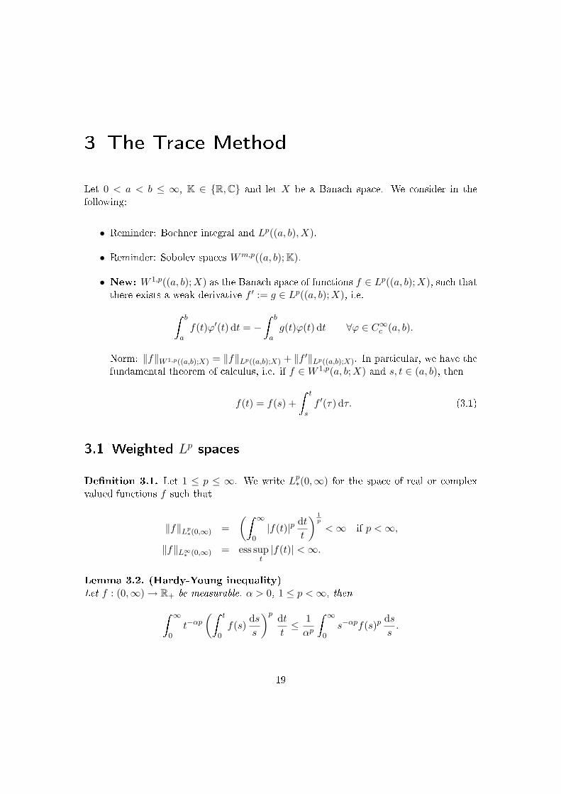
3 The Trace Method
Let 0 < a < b ≤ ∞, K ∈ R,C and let X be a Banach space. We consider in thefollowing:
• Reminder: Bochner integral and Lp((a, b), X).
• Reminder: Sobolev spaces Wm,p((a, b); K).
• New: W 1,p((a, b);X) as the Banach space of functions f ∈ Lp((a, b);X), such thatthere exists a weak derivative f ′ := g ∈ Lp((a, b);X), i.e.
b
af(t)ϕ′(t) dt = −
b
ag(t)ϕ(t) dt ∀ϕ ∈ C∞c (a, b).
Norm: ‖f‖W 1,p((a,b);X) = ‖f‖Lp((a,b);X) + ‖f ′‖Lp((a,b);X). In particular, we have thefundamental theorem of calculus, i.e. if f ∈W 1,p(a, b;X) and s, t ∈ (a, b), then
f(t) = f(s) + t
sf ′(τ) dτ. (3.1)
3.1 Weighted Lp spaces
Denition 3.1. Let 1 ≤ p ≤ ∞. We write Lp∗(0,∞) for the space of real or complexvalued functions f such that
‖f‖Lp∗(0,∞) =
( ∞
0|f(t)|p dt
t
) 1p
<∞ if p <∞,
‖f‖L∞∗ (0,∞) = ess supt|f(t)| <∞.
Lemma 3.2. (Hardy-Young inequality)Let f : (0,∞) → R+ be measurable, α > 0, 1 ≤ p <∞, then
∞
0t−αp
( t
0f(s)
dss
)p dtt≤ 1αp
∞
0s−αpf(s)p
dss.
19
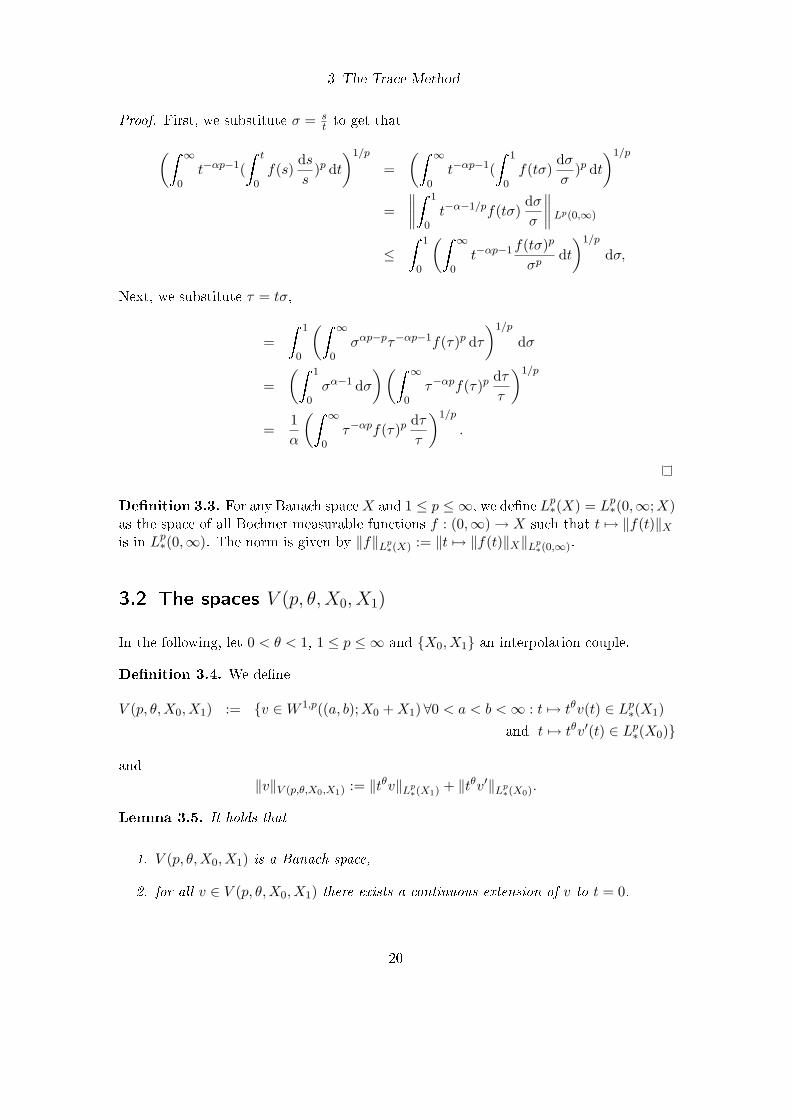
3 The Trace Method
Proof. First, we substitute σ = st to get that
( ∞
0t−αp−1(
t
0f(s)
dss
)p dt)1/p
=( ∞
0t−αp−1(
1
0f(tσ)
dσσ
)p dt)1/p
=∥∥∥∥ 1
0t−α−1/pf(tσ)
dσσ
∥∥∥∥ Lp(0,∞)
≤ 1
0
( ∞
0t−αp−1 f(tσ)p
σpdt)1/p
dσ,
Next, we substitute τ = tσ,
= 1
0
( ∞
0σαp−pτ−αp−1f(τ)p dτ
)1/p
dσ
=( 1
0σα−1 dσ
)( ∞
0τ−αpf(τ)p
dττ
)1/p
=1α
( ∞
0τ−αpf(τ)p
dττ
)1/p
.
Denition 3.3. For any Banach spaceX and 1 ≤ p ≤ ∞, we dene Lp∗(X) = Lp∗(0,∞;X)as the space of all Bochner measurable functions f : (0,∞) → X such that t 7→ ‖f(t)‖Xis in Lp∗(0,∞). The norm is given by ‖f‖Lp
∗(X) := ‖t 7→ ‖f(t)‖X‖Lp∗(0,∞).
3.2 The spaces V (p, θ,X0, X1)
In the following, let 0 < θ < 1, 1 ≤ p ≤ ∞ and X0, X1 an interpolation couple.
Denition 3.4. We dene
V (p, θ,X0, X1) := v ∈W 1,p((a, b);X0 +X1)∀0 < a < b <∞ : t 7→ tθv(t) ∈ Lp∗(X1)and t 7→ tθv′(t) ∈ Lp∗(X0)
and
‖v‖V (p,θ,X0,X1) := ‖tθv‖Lp∗(X1) + ‖tθv′‖Lp
∗(X0).
Lemma 3.5. It holds that
1. V (p, θ,X0, X1) is a Banach space,
2. for all v ∈ V (p, θ,X0, X1) there exists a continuous extension of v to t = 0.
20
3 The Trace Method
Proof. The proof of the rst assertion is given as an exercise. For the second assertion,we use (3.1), the Hölder inequality and the embedding X0 → X0 +X1 to get that for all0 < s < t , 1 < p <∞ and p′ = p
p−1 ,
‖v(t)− v(s)‖X0+X1 ≤ t
s‖τ θ−1/pv′(τ)τ1/p−θ‖X0+X1 dτ
≤( t
s‖τ θ−1/pv′(τ)‖pX0+X1
dτ)1/p( t
sτ (1/p−θ)p′ dτ
)1/p′
≤ C‖v′‖Lp∗(s,t;X1)(1 + p′(1/p− θ))−1/p′(t1+p
′(1/p−θ) − s1+p′(1/p−θ))1/p
′
≤ Cp,θ‖v‖V (θ,p,X0,X1)(t1+p′(1/p−θ) − s1+p
′(1/p−θ))1/p′.
It follows that v : R+ → X0 +X1 is continuous and if we put s = 0 and look at t→ 0 inthe last line, we see that it can be extended continuously to t = 0. The cases p = 1 andp = ∞ are left as an exercise.
3.3 Real interpolation by the trace method and equivalence
Theorem 3.6. Let θ, p and X0, X1 be as above. Then
X := (X0, X1)θ,p = x ∈ X0 +X1 : ∃v ∈ V (p, 1− θ,X1, X0), v(0) = x
and
‖x‖X ∼= infv∈V (p,1−θ,X1,X0),x=v(0)
‖v‖V (p,1−θ,X1,X0) =: ‖x‖TrX
In order to prove this theorem, we want to use the Hardy-Young inequality, through thefollowing lemma.
Lemma 3.7. Let u be a function such that uθ := t 7→ tθu(t) ∈ Lp∗(0, a;X) for some
Banach space X, 0 < a ≤ ∞, 0 < θ < 1 and 1 ≤ p ≤ ∞. Then also the mean value
v(t) :=1t
t
0u(s) ds, t > 0
has this property and ‖vθ‖Lp∗(0,a;X) ≤ 1
1−θ‖uθ‖Lp∗(0,a;X).
Proof. The proof is direct if we use the Hardy-Young inequality, Lemma 3.2, as for1 ≤ p <∞, a
0‖vθ(t)‖pX
dtt
= a
0t(θ−1)p
∥∥∥∥ t
0u(s) ds
∥∥∥∥pX
dtt
≤ a
0t(θ−1)p
( t
0
‖su(s)‖Xs
ds)p dt
t
≤ (1
1− θ)p a
0s(θ−1)p‖su(s)‖pX
dss
= (1
1− θ)p‖uθ‖Lp
∗(0,a;X).
21
3 The Trace Method
The case p = ∞ also follows immediately from the denition.
We can now proceed to the proof of Theorem 3.6.
Proof. First we show that for a given x ∈ X, we can construct a function v ∈ V (p, 1 −θ,X1, X0) such that x is the trace of v in t = 0 and such that ‖x‖TrX ≤ C‖x‖X . Thispart of the proof is devided into four steps.
1. Let x ∈ X. Then for all t > 0 there exist at ∈ X0 and bt ∈ X1 such that x = at+ btand
‖at‖X0 + t‖bt‖X1 ≤ 2K(t, x). (3.2)
It follows that
‖x− bt‖X0+X1 ≤ ‖at‖X0+X1 ≤ C‖at‖X0 ≤ 2CK(t, x) ≤ 2Ctθ‖x‖X
by (2.2). It therefore seems that t 7→ bt would be a candidate for v, but it is notnecessarily dierentiable and it does not necessarily satisfy t1−θbt ∈ Lp(R+;X1) ort1−θb′t ∈ Lp(R+;X0). In the next step, we use bt to construct a suitable candidate.
2. Let
u(t) :=∞∑n=1
b 1n+1
χ( 1n+1
; 1n
](t) =∞∑n=1
(x− a 1n+1
)χ( 1n+1
; 1n
](t)
and let
v(t) =1t
t
0u(s) ds.
Then it still holds that x = limt→0 u(t) = limt→0 v(t) in X0 +X1.
3. We show that v1−θ ∈ Lp∗(R+;X1). Of course, we want to use Lemma 3.7. By (3.2)and from the monotonicity of t 7→ K(t, x), we get
‖t1−θu(t)‖X1 ≤ t−θ∞∑n=1
tχ( 1n+1
, 1n
](t)2(n+ 1)K(
1n+ 1
, x
)≤ 4t−θK(t, x).
It follows that
‖u1−θ‖Lp∗(R+,X1) ≤ 4
( ∞
0(t−θK(t, x))p
dtt
)1/p
= 4‖x‖X , (3.3)
so
‖v1−θ‖Lp∗(R+;X1) ≤ C‖x‖X .
22
3 The Trace Method
4. We show that v′1−θ ∈ Lp∗(R+;X0). We use the following remark, to ensure that we
nd v ∈ W 1,ploc (0,∞, X0 +X1). If on some interval I ⊂ R we have f, g ∈ L1(I; R)
and
f(x)− f(y) = y
xg(s) ds
for almost all x, y ∈ I, then f ∈ W 1,1(I; R) and g is its weak derivative, as forc, d ∈ I and all ϕ ∈ C∞c (I) with supp(ϕ) ∈ [c, d],
d
cϕ′(y)(f(y)−f(c)) dy =
d
c
y
cϕ′(y)g(x) dxdy =
d
c
d
xϕ′(y) dyg(x) dx = −
d
cϕ(x)g(x) dx.
We use this fact on ‖v(t)‖X0+X1 and that, by denition,
v(t) = x− 1t
t
0
∞∑n=1
a 1n+1
χ( 1n+1
, 1n
](s) ds
and
v′(t) =1t2
t
0g(s) ds− 1
tg(t)
holds true almost everywhere for g(t) :=∑∞
n=1 a 1n+1
χ( 1n+1
, 1n
](t) ∈ X0. Again, from
the monotonicity of t 7→ K(t, x), it follows that
‖g(t)‖X0 ≤∞∑n=1
2K(
1n+ 1
, x
)χ( 1
n+1, 1n
](t) ≤ 2K(t, x)
and therefore
‖t1−θv′(t)‖X0 ≤ t1−θ
t2
t
0‖g(s)‖X0 ds+ t−θ‖g(t)‖X0
≤ 4t−θK(t, x).
As in (3.3), it follows that ‖v1−θ‖Lp∗(R+;X0) ≤ C‖x‖X . In conclusion, we see that
v ∈ V (p, 1 − θ,X1, X0), that x = limt→0 v(t) in X0 + X1 and that ‖x‖TrX ≤‖v‖V (p,1−θ,X1,X0) ≤ C‖x‖X .
We now look at the opposite inclusion and assume that x ∈ X0 + X1 is the trace of afunction v ∈ V (p, 1− θ,X1, X0) at t = 0. We can write
x = x− v(t) + v(t) = − t
0v′(s) ds+ v(t), t > 0,
cf. Lemma 3.5. Therefore, we see that
t−θK(t, x) ≤ t1−θ‖1t
t
0v′(s) ds‖X0 + t1−θ‖v(t)‖X1 , t > 0.
23
3 The Trace Method
By Lemma 3.7,
‖x‖X = ‖t−θK(t, x)‖Lp∗(R+) ≤ C‖v′1−θ‖Lp
∗(R+;X0) +‖v1−θ‖Lp∗(R+,X1) ≤ C‖v‖V (p,1−θ,X1,X0).
Remark 3.8. Let x ∈ (X0, X1)θ,p be the trace of a function v ∈ V (p, 1− θ,X1, X0).
1. We can improve the regularity of v in the following way: For any smooth non-negative function ϕ : R+ 7→ R with compact support and
∞0 ϕ(s) ds
s = 1, weset
u(t) = ∞
0ϕ(t
τ)v(τ)
dττ
= ∞
0ϕ(s)v(
t
s)dss.
Then we get u ∈ C∞(R+;X0 ∩X1), u(0) = x and
t 7→ tn−θu(n)(t) ∈ Lp∗(R+;X0), n ∈ N,t 7→ tn+1−θu(n)(t) ∈ Lp∗(R+;X1), n ∈ N ∪ 0,
with norms estimated by c(n)‖v‖V (p,1−θ,X1,X0). The proof is left as an exercise.
2. Let ψ ∈ C∞c ([0,∞)) such that ψ ≡ 1 in (0, 1] or any right neighbourhood of 0. Thenuψ : t 7→ ψ(t)u(t) ∈ V (p, 1 − θ,X1, X0) with trace x at t = 0, where u is chosenas in 1. Moreover, ‖uψ‖V (p,1−θ,X1,X0) ≤ Cψ‖u‖V (p,1−θ,X1,X0) and it has compactsupport. This shows that we could also consider a subset of V (p, 1 − θ,X1, X0)consisting of functions with compact support in order to dene an equivalent tracespace.
Corollary 3.9. Let 1 < p <∞. Then (X0, X1)1−1/p,p is the set of the traces at t = 0 of
the functions u ∈W 1,p(0,∞;X1) ∩ Lp(0,∞;X0).
Proof. Clearly, if θ = 1 − 1/p, u1−θ ∈ Lp∗(R+;Xi) i u ∈ Lp(R+;Xi). The corollaryfollows if we take into account Remark 3.8.
The following example gives us an important motivation to consider the trace method.
Example 3.10. Let Rn+1+ denote the upper half-space (t, x) ∈ R × Rn : t > 0.
Then for 1 < p < ∞, (Lp(Rn),W 1,p(Rn))1−1/p,p is the space of traces of functions
(t, x) 7→ v(t, x) ∈W 1,p(Rn+1+ ) at t = 0.
We close this chapter with a theoretical result on the real interpolation space X =(X0, X1)θ,p which can be derived by the trace method.
Proposition 3.11. Let 0 < θ < 1 and X0, X1 an interpolation couple. For 1 ≤ p <∞,
X0 ∩X1 is dense in X = (X0, X1)θ,p.
24
3 The Trace Method
Proof. Let x ∈ X. By Remark 3.8, x = v(0), where v ∈ C∞(R+;X0 ∩ X1) ∩ V (p, 1 −θ,X1, X0) and t 7→ t2−θv′ ∈ Lp∗(R+, X1). We set
xε := v(ε) ∈ X0 ∩X1, ∀ε > 0
and show that xε → x in X. We dene
zε(t) := (v(ε)− v(t))χ[0,ε](t)
to get xε−x = zε(0), zε ∈W 1,p(a, b;X0) for all 0 < a < b <∞ and z′ε(t) = −v′(t)χ(0,ε)(t).It follows that
limε→0
‖t1−θz′ε(t)‖Lp∗(R+;X0) = 0.
We now show that t 7→ t1−θzε(t) ∈ Lp∗(R+;X1) by using
zε(t) = ∞
tχ(0,ε)(s)v
′(s) ds
and a modied version of the Hardy-Young inequality: For α > 0, p ≥ 1 and positive ϕ,we have that ∞
0tαp(
∞
tϕ(s)
dss
)pdtt≤ 1αp
∞
0sαpϕ(s)p
dss, (3.4)
which follows from Lemma 3.2 by substituting τ = 1t and σ = 1
s . We get that
∞
0(t1−θ‖zε(t)‖X1)
p dtt
≤ ∞
0t(1−θ)p(
∞
tχ(0,ε)(s)s‖v′(s)‖X1
dss
)pdtt
≤ (1
1− θ)p ∞
0χ(0,ε)(s)s
(2−θ)p‖v′(s)‖pX1
dss,
so thatlimε→0
‖t1−θzε(t)‖Lp∗(R+;X1) = 0.
In conclusion, zε → 0 in V (p, 1 − θ,X1, X0) as ε → 0, so ‖xε − x‖TrX → 0 as ε → 0. ByTheorem 3.6, limε→0 ‖xε − x‖X = 0.
25
4 The Reiteration Theorem
In the following, let X0, X1 an interpolation couple. We dene two classes of interme-diate spaces.
Denition 4.1. Let 0 ≤ θ ≤ 1 and let X be a Banach space such that X0∩X1 → X →X0 +X1.
1. We say that X belongs to the class Jθ between X0 and X1 if there exists a constantc > 0 such that
‖x‖X ≤ c‖x‖1−θX0
‖x‖θX1, ∀x ∈ X0 ∩X1.
We write X ∈ Jθ(X0, X1).
2. We say that X belongs to the class Kθ between X0 and X1 if there is a constantk > 0 such that
K(t, x,X0, X1) ≤ ktθ‖x‖X , ∀x ∈ X, t > 0.
In this case we write X ∈ Kθ(X0, X1). If θ ∈ (0, 1), this means that X →(X0, X1)θ,∞.
Proposition 4.2. Let θ ∈ (0, 1) and let X be an intermediate space for X0, X1. Thenthe following statements are equivalent:
1. X ∈ Jθ(X0, X1),
2. (X0, X1)θ,1 → X.
Proof. The implication 2. ⇒ 1. follows directly from Theorem 2.5 (5) with q = 1. Weshow that 1.⇒ 2.. For every x ∈ (X0, X1)θ,1, let u ∈ V (1, 1− θ,X1, X0)∩C∞(R+;X1 ∩X0) such that u(t) → 0 as t→∞ and u(0) = x. We set
v(t) =1t
t
0u(s) ds,
so that t 7→ t2−θv′(t) ∈ L1∗(R+;X1) and t 7→ t1−θv′(t) ∈ L1
∗(R+;X0) follows, similarly asin Remark 3.8, by Lemma 3.7. It still holds that v(0) = x and that v(t) → 0 as t→∞,so
x = − ∞
0v′(t) dt.
26
4 The Reiteration Theorem
Let c be such that ‖y‖X ≤ c‖y‖θX1‖y‖1−θ
X0for every y ∈ X0 ∩X1. Then
‖v′(t)‖X ≤ c‖v′(t)‖θX1‖v′(t)‖1−θ
X0= ct−1‖t2−θv′(t)‖θX1
‖t1−θv′(t)‖1−θX0
.
Now by Hölder's inequality, as 1 = 11/θ + 1
1/(1−θ) ,
‖x‖X ≤ ‖v′‖L1(R+;X) ≤ c∥∥∥t−θ‖t2−θv′(t)‖θX1
t−(1−θ)‖t1−θv′(t)‖1−θX0
∥∥∥ L1(R+).
≤ c‖t2−θv′(t)‖θL1∗(R+,X1)‖t
1−θv′(t)‖1−θL1∗(R+,X0)
≤ c‖x‖(X0,X1)θ,1.
The above proposition shows that for θ ∈ (0, 1), X ∈ Jθ(X0, X1) ∩ Kθ(X0, X1) i(X0, X1)θ,1 → X → (X0, X1)θ,∞.
Example 4.3. Actually, two examples:
1. By Equation (2.2) and by Theorem 2.5, (X0, X1)θ,p ∈ Kθ(X0, X1) ∩ Jθ(X0, X1).
2. The space C1([−1, 1]) lies in
K1/2(C([−1, 1]), C2([−1, 1])) ∩ J1/2(C([−1, 1]), C2([−1, 1])),
but, as we have seen, it is not an interpolation space. The proof is left as anexercise.
The following theorem shows that we can iterate the procedure of interpolating spaces,i.e. the real interpolation spaces of two suitable intermediate spaces is again a realinterpolation space.
Theorem 4.4. (Reiteration Theorem)Let 0 ≤ θ0 < θ1 ≤ 1. We x θ ∈ (0, 1) and set ω = (1 − θ)θ0 + θθ1. Then the following
holds true.
1. If for an interpolation couple X0, X1, there are intermediate spaces Ei ∈ Kθi(X0, X1),
i ∈ 0, 1, then
(E0, E1)θ,p → (X0, X1)ω,p for all 1 ≤ p ≤ ∞.
2. If on the other hand, Ei ∈ Jθi(X0, X1), then
(X0, X1)ω,p → (E0, E1)θ,p.
27
4 The Reiteration Theorem
In conclusion, if Ei ∈ Jθi(X0, X1) ∩Kθi
(X0, X1), then
(E0, E1)θ,p = (X0, X1)ω,p for all 1 ≤ p ≤ ∞,
with equivalence of the respective norms.
Proof. We rst show 1.:Let ki be such that
K(t, e,X0, X1) ≤ kitθi‖e‖Ei , e ∈ Ei, t > 0.
Let e0 ∈ E0 and e1 ∈ E1 be such that e = e0 + e1. It follows that
K(t, e,X0, X1) ≤ K(t, e0, X0, X1) +K(t, e1, X0, X1) ≤ k0tθ0‖e0‖E0 + k1t
θ1‖e1‖E1 .
Taking the inmum, it follows that
K(t, e,X0, X1) ≤ maxk0, k1tθ0(‖e0‖E0 + tθ1−θ0‖e1‖E1)≤ maxk0, k1tθ0K(tθ1−θ0 , e, E0, E1),
so we get
t−ωK(t, e,X0, X1) ≤ maxk0, k1t−θ(θ1−θ0)K(tθ1−θ0 , e, E0, E1).
Setting s = tθ1−θ0 , we can conclude
‖e‖(X0,X1)ω,p≤ maxk0, k1‖s−θK(s, e, E0, E1)‖Lp
∗(0,∞) = maxk0, k1‖e‖(E0,E1)θ,p,
if p <∞ and‖e‖(X0,X1)ω,∞ ≤ maxk0, k1‖e‖(E0,E1)θ,p
.
We now show 2.:By Theorem 3.6 and Remark 3.8, every x ∈ (X0, X1)ω,p is the trace at t = 0 of a functionv ∈ C∞(R+, X0 ∩X1) such that v(∞) = 0, v′1−ω ∈ L
p∗(R+, X0), v′2−ω ∈ L
p∗(R+, X1) and
‖v′1−ω‖Lp∗(R+,X0) + ‖v′2−ω‖Lp
∗(R+,X1) ≤ k‖x‖Tr(X0,X1)ω,p. (4.1)
We now consider the functiong(t) = v(t1/(θ1−θ0))
and show that it belongs to V (p, 1 − θ, E1, E0), so that g(0) = v(0) = x ∈ (E0, E1)θ,pwith the corresponding estimate.First, we look at ‖v′(t)‖Ei , t > 0, i ∈ 0, 1. Let ci such that
‖x‖Ei ≤ ci‖x‖1−θiX0
‖x‖θiX1, x ∈ X0 ∩X1.
We get
‖v′(t)‖Ei ≤ci
t1+θi−ω‖t1−ωv′(t)‖1−θi
X0‖t2−ωv′(t)‖θi
X1.
28
4 The Reiteration Theorem
Now we calculate
1 + θ0 − ω = 1 + θ0 − (1− θ)θ0 − θθ1 = 1− θ(θ1 − θ0)
and1 + θ1 − ω = 1 + θ1 − (1− θ)θ0 − θθ1 = 1 + (1− θ)(θ1 − θ0)
to obtain that‖v′1−θ(θ1−θ0)‖Lp
∗(0,∞,E0) ≤ c0k‖x‖Tr(X0,X1)ω,p(4.2)
and that‖v′1+(1−θ)(θ1−θ0)‖Lp
∗(0,∞,E1) ≤ c1k‖x‖Tr(X0,X1)ω,p(4.3)
by Hölder's inequality and (4.1). We now use
v(t) = − ∞
tv′(s) ds (4.4)
and the second Hardy-Young inequality (3.4) to get that
‖v(1−θ)(θ1−θ0)‖Lp∗(0,∞,E1)
(4.4)
≤( ∞
0t(1−θ)(θ1−θ0)p
( ∞
t‖sv′(s)‖E1
dss
)p dtt
)1/p
(3.4)
≤ 1(1− θ)(θ1 − θ0)
( ∞
0s(1−θ)(θ1−θ0)p+p‖v′(s)‖pE1
dss
)1/p
(4.3)
≤ 1(1− θ)(θ1 − θ0)
c1k‖x‖Tr(X0,X1)ω,p.
With the substitution s = t1/(θ1−θ0), i.e. t = sθ1−θ0 and dt = (θ1 − θ0)s(θ1−θ0)−1 ds, itfollows that
‖g1−θ‖Lp∗(0,∞,E1) =
( ∞
0t(1−θ)p‖v(t1/(θ1−θ0))‖pE1
dtt
)1/p
=( ∞
0s(θ1−θ0)(1−θ)p‖v(s)‖pE1
(θ1 − θ0)dss
)1/p
= (θ1 − θ0)1/p‖v(1−θ)(θ1−θ0)‖Lp∗(0,∞,E1)
≤ (1− θ)−1(θ1 − θ0)1/p−1c1k‖x‖Tr(X0,X1)ω,p.
Similarly, we look at
g′(t) = (θ1 − θ0)−1t(1/(θ1−θ0)−1)v′(t1/(θ1−θ0))
to get that
‖g′1−θ‖Lp∗(0,∞,E0) =
1θ1 − θ0
( ∞
0(t1−θ+1/(θ1−θ0)−1‖v′(t1/(θ1−θ0))‖E0)
p dtt
)1/p
s=t1/(θ1−θ0)
= (θ1 − θ0)1/p−1‖v′1−θ(θ1−θ0)‖Lp∗(0,∞,E0)
(4.2)
≤ c0k(θ1 − θ0)1/p−1‖x‖Tr(X0,X1)ω,p.
29
4 The Reiteration Theorem
In conclusion, we get that g ∈ V (p, 1 − θ, E1, E0), so that x = g(0) ∈ (E0, E1)θ,p byTheorem 3.6 and
‖x‖(E0,E1)θ,p≤ ‖g‖V (p,1−θ,E1,E0) ≤ maxcik(1− θ)−1(θ1 − θ0)1/p−1‖x‖Tr(X0,X1)ω,p
= maxcik(θ1 − θ0)1/p
(θ1 − ω)‖x‖Tr(X0,X1)ω,p
.
Corollary 4.5. From Theorem 4.4 and Example 4.3 we immediately get that for any
0 < θ0 < θ1 < 1, 0 < θ < 1 and 1 ≤ p, q0, q1 ≤ ∞,
((X0, X1)θ0,q0 , (X0, X1)θ1,q1)θ,p = (X0, X1)(1−θ)θ0+θθ1,p.
30
5 Complex Interpolation
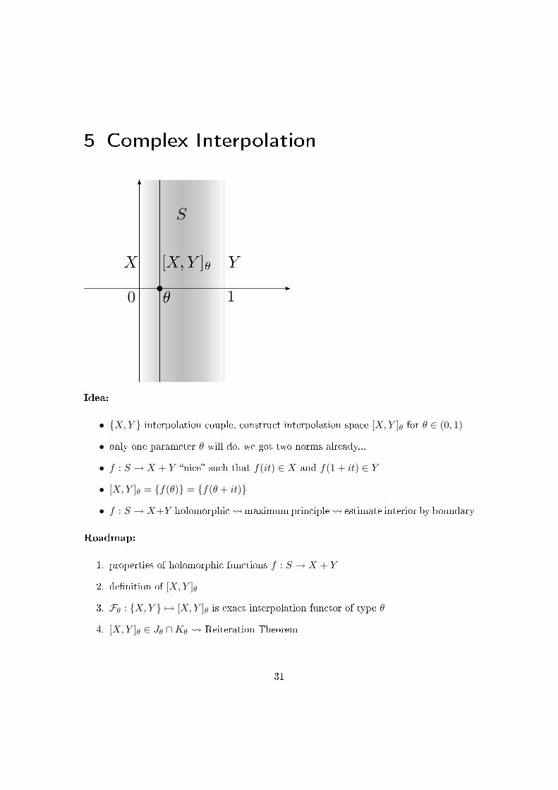
Idea:
• X,Y interpolation couple, construct interpolation space [X,Y ]θ for θ ∈ (0, 1)
• only one parameter θ will do, we got two norms already...
• f : S → X + Y nice such that f(it) ∈ X and f(1 + it) ∈ Y
• [X,Y ]θ = f(θ) = f(θ + it)
• f : S → X+Y holomorphic maximum principle estimate interior by boundary
Roadmap:
1. properties of holomorphic functions f : S → X + Y
2. denition of [X,Y ]θ
3. Fθ : X,Y 7→ [X,Y ]θ is exact interpolation functor of type θ
4. [X,Y ]θ ∈ Jθ ∩Kθ Reiteration Theorem
31
5 Complex Interpolation
5.1 X-valued holomorphic functions
Let X be a complex Banach space. For every set Ω ⊂ C we say that f : Ω → X isholomorphic in S ⊂ Ω, if f is dierentiable in every λ0 in a neighbourhood of S, i.e. thelimit
f ′(λ0) = limλ→λ0
f(λ)− f(λ0)λ− λ0
exists in X.
Proposition 5.1. Let Ω ⊂ C be a bounded open set and f : Ω → X a function which is
holomorphic on Ω and continuous on Ω. Then
‖f(ξ)‖X ≤ max‖f(z)‖X : z ∈ ∂Ω ∀ξ ∈ Ω.
Proof. For every ξ ∈ Ω we can choose x′(ξ) ∈ X ′ in the dual space of X such that‖f(ξ)‖X = 〈f(ξ), x′(ξ)〉 and ‖x′(ξ)‖X′ = 1. We apply the maximum principle for C-valued holomorphic functions to z 7→ 〈f(z), x′(ξ)〉 to get
‖f(ξ)‖X = |〈f(ξ), x′(ξ)〉| ≤ max|〈f(z), x′(ξ)〉|, z ∈ ∂Ω≤ max‖f(z)‖X , z ∈ ∂Ω.
Following the idea above, we want to consider holomorphic functions on the strip
S := x+ iy ∈ C : 0 ≤ x ≤ 1.
Also for this set, the maximum principle holds.
Proposition 5.2. Let f : S → X be holomorphic onS and continuous and bounded on
S. Then
‖f(ξ)‖X ≤ maxsupt∈R
‖f(it)‖X , supt∈R
‖f(1 + it)‖X.
Proof. Let ε ∈ (0, 1) and ξ0 = x0 + it0 ∈ S such that
‖f(ξ0)‖ ≥ (1− ε)‖f‖C(S,X).
We set fδ(ξ) := eδ(ξ−ξ0)2f(ξ), ξ = x+ it, so that fδ(ξ0) = f(ξ0) and
lim|t|→∞
eδ(x+it−ξ0)2f(ξ) = lim|t|→∞
e−δt2+2δ(it)(x−ξ0)+δ(x−ξ0)2f(ξ)
= lim|t|→∞
e−δt(t−2t0)eδRe(x−ξ0)2f(ξ)
= 0.
32
5 Complex Interpolation
We can now apply the maximum principle, Proposition 5.1, to fδ on every domain [0, 1]×[−M,M ], M > 0. By the above calculation, for large M , only the vertical boundarieswill be relevant.
‖fδ(ξ)‖ ≤ maxsupt∈R
‖fδ(it)‖, supt∈R
‖fδ(1 + it)‖
≤ maxeδRe(1−ξ0)2 , eδRe ξ20 supt∈R
e−δt(t−2t0)maxsupt∈R
‖f(it)‖, supt∈R
‖f(1 + it)‖.
It is easy to show that supt∈R e−δt(t−2t0) = eδt
20 is reached in t = t0, so that in conclusion,
for every ε ∈ (0, 1) there exists a suciently small δ such that
(1− ε)‖f‖C(S,X) ≤ ‖f(ξ0)‖ = ‖fδ(ξ0)‖≤ (1 + ε) maxsup
t∈R‖f(it)‖, sup
t∈R‖f(1 + it)‖.
Theorem 5.3. (Three lines theorem)
Let f : S → X be holomorphic onS and continuous and bounded on S. Then for all
0 < θ < 1, we have
‖f(θ)‖X ≤ (supt∈R
‖f(it)‖X)1−θ(supt∈R
‖f(1 + it)‖X)θ.
Proof. In the following, we use the abbreviations M0 := supt∈R ‖f(it)‖X and M1 :=supt∈R ‖f(1+it)‖X and we consider the function ϕ(z) = eλzf(z) where λ = log(M0/M1).By the maximum principle on S, Proposition 5.2,
‖f(θ)‖X = |e−λθ|‖ϕ(θ)‖θ‖ϕ(θ)‖1−θ
≤ (M1
M0)θ maxeλitM0, e
λ+λitM1θ maxeλitM0, eλ+λitM11−θ
= (M1
M0)θM θ
0M1−θ0
= M1−θ0 M θ
1 .
5.2 The spaces [X, Y ]θ and basic properties
Denition 5.4. The space G(X,Y ) is dened as the space of all functions f : S → X+Ysuch that
1. f is holomorphic inS and continuous and bounded on S with values in X + Y .
33
5 Complex Interpolation
2. It holds that t 7→ f(it) ∈ Cb(R;X), t 7→ f(1 + it) ∈ Cb(R;Y ) and
‖f‖G(X,Y ) = maxsupt∈R
‖f(it)‖X , supt∈R
‖f(1 + it)‖Y <∞.
G0(X,Y ) is a subspace of G(X,Y ) which imposes the additional properties
lim|t|→∞
‖f(it)‖X = 0, lim|t|→∞
‖f(1 + it)‖Y = 0.
In the exercises, we show that both G(X,Y ) and G0(X,Y ) are Banach spaces, continu-ously embedded in Cb(S,X + Y ).
We only cite the following technical lemma. (The reason is: the proof is dicult)
Lemma 5.5. The linear hull of the set of functions z 7→ eδz2+λza, δ > 0, λ ∈ R,
a ∈ X ∩ Y , is dense in G0(X,Y ).
Denition 5.6. (Complex Interpolation Spaces)For every θ ∈ [0, 1], we set
[X,Y ]θ := f(θ) : f ∈ G(X,Y ),‖x‖[X,Y ]θ := inf
f∈G(X,Y ),f(θ)=x‖f‖G(X,Y ).
We see that [X,Y ]θ is a Banach space from the fact that it is isomorphic to the quotientspace G(X,Y )/Nθ, where Nθ is the closed subspace of functions f ∈ G(X,Y ), satisfyingf(θ) = 0.
Proposition 5.7. (Properties of [X,Y ]θ)
1. If θ ∈ (0, 1), it holds that [X,Y ]θ = [Y,X]1−θ.
2. The space [X,Y ]θ can be dened equivalently from the space G0(X,Y ).
3. If X = Y , then [X,X]θ = X.
4. For every t ∈ R and f ∈ G(X,Y ), f(θ + it) ∈ [X,Y ]θ for every θ ∈ (0, 1) and
‖f(θ + it)‖[X,Y ]θ = ‖f(θ)‖[X,Y ]θ .
5. For every θ ∈ (0, 1), we get that [X,Y ]θ is an intermediate space of X,Y , i.e.
X ∩ Y → [X,Y ]θ → X + Y.
6. For every θ ∈ (0, 1), X ∩ Y is dense in [X,Y ]θ.
Proof.
34
5 Complex Interpolation
1. Follows directly from the denition (reect fs)
2. For every f ∈ G(X,Y ) and δ > 0, we can dene fδ(z) = eδ(z−θ)2f(z). We already
know this function, that fδ(θ) = f(θ) and that it lies in G0(X,Y ). By denition,
‖fδ‖G(X,Y ) ≤ maxeδθ2 , eδ(1−θ)2‖f‖G(X,Y ),
from δ → 0, we see
inff∈G(X,Y ),f(θ)=x
‖f‖G(X,Y ) = inff∈G0(X,Y ),f(θ)=x
‖f‖G(X,Y ).
3. This follows from the maximum principle. For x ∈ [X,X]θ, we have
‖x‖X = ‖f(θ)‖Xm.p.≤ ‖f‖G(X,X).
Taking the inf gives ‖x‖X ≤ ‖x‖[X,X]θ . On the other hand, the constant functioncx : z 7→ x, z ∈ S is in G(X,X), so that for every x ∈ X, ‖x‖X = ‖cx‖G(X,X) ≥‖x‖[X,X]θ .
4. Let g(z) = f(z + it). We see directly that g ∈ G(X,Y ) and that ‖g‖G(X,Y ) =‖f‖G(X,Y ). It follows that f(θ + it) = g(θ) ∈ [X,Y ]θ and that the norm doesn'tchange.
5. Let x ∈ X ∩ Y . Again, the constant function cx(z) = x belongs to G(X,Y ) and
‖cx‖G(X,Y ) ≤ max‖x‖X , ‖x‖Y ,
so that x = cx(θ) ∈ [X,Y ]θ and ‖x‖[X,Y ]θ ≤ ‖x‖X∩Y .On the other hand, if x = f(θ) ∈ [X,Y ]θ, then
‖x‖X+Y ≤ ‖f(θ)‖X+Ym.p.≤ maxsup
t∈R‖f(it)‖X+Y , sup
t∈R‖f(1 + it)‖X+Y
≤ Cmaxsupt∈R
‖f(it)‖X , supt∈R
‖f(1 + it)‖Y
= C‖f‖G(X,Y ).
Taking the inmum, we get ‖x‖X+Y ≤ C‖x‖[X,Y ]θ .
6. This follows directly from Lemma 5.5. For every x ∈ [X,Y ]θ, there is a functionf ∈ G0(X,Y ) such that f(θ) = x, by 2. By Lemma 5.5, there is a sequence offunctions given by
fn(z) =mn∑i=1
µieδiz
2+λizai ∈ X ∩ Y
such that fn → f in G0(X,Y ). Setting xn = fn(θ), we have ‖x − xn‖[X,Y ]θ =‖f(θ)− fn(θ)‖[X,Y ]θ ≤ ‖f − fn‖G0(X,Y ).
35
5 Complex Interpolation
Proposition 5.8. We let V (X,Y ) the linear hull of the functions z 7→ ϕ(z)x, S → X∩Y ,where ϕ ∈ G0(C,C) and x ∈ X ∩ Y . For every x ∈ X ∩ Y , we get
‖x‖[X,Y ]θ = inff∈V (X,Y ),f(θ)=x
‖f‖G(X,Y ).
Proof. We can approximate the norm of x by choosing for every ε > 0 a function f0 ∈G0(X,Y ) such that x = f0(θ) and ‖f0‖G(X,Y ) ≤ ‖x‖[X,Y ]θ + ε. We dene a functionr ∈ G(C,C) by
r(z) =z − θ
z + θ, z ∈ S
and set
f1(z) =f0(z)− e(z−θ)
2x
r(z), z ∈ S.
It follows that f1 ∈ G0(X,Y ), as f0 ∈ G0(X,Y ), z 7→ e(z−θ)2x ∈ G0(X,Y ) and |r(z)| ≤
1, r(z) 6= 0 if z 6= 0 and r′(θ) 6= 0. By Lemma 5.5, it follows that there exists anapproximating function
f2(z) =n∑i=1
µieδiz
2+λizxi
with δi > 0, λi ∈ R and xi ∈ X ∩ Y such that ‖f1 − f2‖G(X,Y ) ≤ ε. We now set
f(z) = e(z−θ)2x+ r(z)f2(z), z ∈ S.
It follows that f ∈ V (X,Y ) and that
‖f‖G(X,Y ) ≤ ‖f0‖G(X,Y ) + ‖f − f0‖G(X,Y )
≤ ‖x‖[X,Y ]θ + ε+ ‖e(·−θ)2x+ rf1 − f0‖G(X,Y ) + ‖r(f2 − f1)‖G(X,Y )
≤ ‖x‖[X,Y ]θ + 2ε.
5.3 The complex interpolation functor
Theorem 5.9. For every θ ∈ (0, 1),
Fθ : C′2 → C′1, X,Y 7→ [X,Y ]θ
is an exact interpolation functor of type θ, where C′i denotes the categories containing
complex Banach spaces and complex interpolation couples.
36
5 Complex Interpolation
Proof. Let X,Y , X,Y be complex interpolation couples and T ∈ L(X,X, Y, Y ).For every x ∈ [X,Y ]θ, let f ∈ G(X,Y ) such that f(θ) = x. We set
g(z) =
(‖T‖L(X,X)
‖T‖L(Y,Y )
)z−θTf(z), z ∈ S.
It follows that g ∈ G(X,Y ) and that
‖g(it)‖X ≤ ‖T‖1−θL(X,X)
‖T‖θL(Y,Y )‖f(it)‖X ,
‖g(1 + it)‖Y ≤ ‖T‖1−θL(X,X)
‖T‖θL(Y,Y )‖f(1 + it)‖Y .
Therefore, ‖g‖G(X,Y ) ≤ ‖T‖1−θL(X,X)
‖T‖θL(Y,Y )‖f‖G(X,Y ) and so Tx = g(θ) ∈ [X,Y ]θ. We
have the estimate
‖Tx‖[X,Y ]θ≤ ‖g‖G(X,Y ) ≤ ‖T‖1−θ
L(X,X)‖T‖θL(Y,Y )
‖f‖G(X,Y ),
so that by taking the inmum over f , we get ‖T‖L([X,Y ]θ,[X,Y ]θ) ≤ ‖T‖1−θL(X,X)
‖T‖θL(Y,Y ).
Following the ideas for Theorem 5.9, we can prove the following result.
Theorem 5.10. Let X,Y , X,Y again be interpolation couples. For every z ∈ Slet Tz ∈ L(X ∩ Y,X + Y ) be such that z 7→ Tzx is in G(X,Y ) for every x ∈ X ∩ Y .Moreover, assume that Tit ∈ L(X,X) and that T1+it ∈ L(Y, Y ). Assume further that the
following suprema are nite:
M0 := supt∈R
‖Tit‖L(X,X), M1 := supt∈R
‖T1+it‖L(Y,Y ).
In this case, for every θ ∈ (0, 1), we get
‖Tθx‖[X,Y ]θ≤M1−θ
0 M θ1 ‖x‖[X,Y ]θ ,
so that Tθ extends to an operator in L([X,Y ]θ, [X,Y ]θ).
Proof. The proof is an exercise, using the proof of Theorem 5.9 and Proposition 5.8.
5.4 The space [X, Y ]θ is of class Jθ and of class Kθ.
Corollary 5.11. For every θ ∈ (0, 1) we have
‖y‖[X,Y ]θ ≤ ‖y‖1−θX ‖y‖θY , y ∈ X ∩ Y,
i.e. [X,Y ]θ ∈ Jθ(X,Y ).
37
5 Complex Interpolation
Proof. The idea is the same as for real interpolation spaces. We consider the operatorsTyλ = λy, T ∈ L(C,C, X,Y ) and use Theorem 5.9, i.e. the exactness of theinterpolation functor, to get
‖y‖[X,Y ]θ = ‖Ty‖L(C,[X,Y ]θ) ≤ ‖y‖1−θX ‖y‖θY .
To prove that [X,Y ]θ ∈ Kθ(X,Y ) needs more work. The main idea is to use a Poissonintegral formula for Banach-space valued holomorphic functions on the strip S.
Theorem 5.12. For θ ∈ (0, 1), the spaces [X,Y ]θ are in the class Kθ(X,Y ).
Proof. We do not give a detailed proof, but name the basic steps and ingredients.
1. Preliminary observation: for a ∈ [X,Y ]θ, in order to estimate
K(t, a,X, Y ) = infa=x+y
‖x‖X + t‖y‖Y ,
we split a and therefore f ∈ G(X,Y ) with a = f(θ) into f = fX + fY , wherefX : S → X, fY : S → Y , recovering estimates for fX and fY in terms of theboundary values f(it), f(1 + it).
2. The Poisson formula: The Dirichlet problem on the open unit ball D, given by
∆u = 0, in D,
u(λ) = h(λ), on ∂D, (5.1)
can be solved by the Poisson formula
u(ξ) =12π
|λ|=1
h(λ)1− |ξ|2
|ξ − λ|2dλ. (5.2)
If h is continuous, u is unique. Therefore if f is holomorphic on D and boundedon ∂D, it satises (5.2) with u = f and h = f |∂D.
3. The solution formula (5.2) transfers from D to S: By the Riemannian MappingTheorem, this will work for all connected open subsets of C. If there is a conformalmap ϕ : Ω → D, then the Dirichlet problem (5.1) is equivalent to the Dirichletproblem
∆v = 0, in Ω,v(ω) = (h ϕ)(ω), on ∂Ω
and v = u ϕ. In particular,
ξ(z) =eπiz − i
eπiz + i, z ∈ S,
38
5 Complex Interpolation
is a conformal map from S to D. The Poisson formula for S is thus given by
v(z) = ∞
−∞eπ(y−t) sin(πx)
[h(it)
sin2(πx) + (cos(πx)− eπ(y−t))2
+h(1 + it)
sin2(πx) + (cos(πx) + eπ(y−t))2
]dt, (5.3)
where z = x+ iy ∈S and it is satised by every function f ∈ G(C,C) with v and
h replaced by f .
4. It follows from the Hahn-Banach theorem, that equation (5.3) also holds in X + Yfor f ∈ G(X,Y ), as for every z′ ∈ (X + Y )′, the function fz′ : z 7→ 〈f(z), z′〉 isholomorphic and satises (5.3). In particular, we can write f = fX + fY , where
fX(z) = ∞
−∞eπ(y−t) sin(πx)
f(it)sin2(πx) + (cos(πx)− eπ(y−t))2
dt, (5.4)
fY (z) = ∞
−∞eπ(y−t) sin(πx)
f(1 + it)sin2(πx) + (cos(πx) + eπ(y−t))2
dt. (5.5)
5. The two kernels in (5.4) and (5.5) are positive and we have that
∞
−∞eπ(y−t) sin(πx)
[1
sin2(πx) + (cos(πx)− eπ(y−t))2
+1
sin2(πx) + (cos(πx) + eπ(y−t))2
]dt = 1,
from considering f ≡ 1, so that
0 <
∞
−∞eπ(y−t) sin(πx)
1sin2(πx) + (cos(πx)− eπ(y−t))2
dt < 1,
0 <
∞
−∞eπ(y−t) sin(πx)
1sin2(πx) + (cos(πx) + eπ(y−t))2
dt < 1.
It follows that
‖fX(z)‖X ≤ supτ∈R
‖f(iτ)‖X , z ∈ S and
‖fY (z)‖Y ≤ supτ∈R
‖f(1 + iτ)‖Y , z ∈ S.
6. From these estimates we get that for every t > 0, f ∈ G(X,Y ) and f(θ) = a ∈[X,Y ]θ,
K(t, a,X, Y ) ≤ ‖fX(θ)‖X + t‖fY (θ)‖Y ≤ supτ∈R
‖f(iτ)‖X + t supτ∈R
‖f(1 + iτ)‖Y .
39
5 Complex Interpolation
For every f , we can also apply this estimate to the function g : z 7→ tθ−zf(z), whichis also in G(X,Y ) with g(θ) = a, to get that
K(t, a) ≤ tθ supτ∈R
‖f(iτ)‖X + tθ−1t supτ∈R
‖f(1 + iτ)‖Y ≤ 2tθ‖f‖G(X,Y ).
Taking the inmum over f yields the claim.
Corollary 5.13. It follows that for every 0 < θ, θ0, θ1 < 1, 1 ≤ p ≤ ∞, we have
([X,Y ]θ0 , [X,Y ]θ1)θ,p = (X,Y )θ0(1−θ)+θθ1,p
and that
(X,Y )θ,1 → [X,Y ]θ → (X,Y )θ,∞.
Remark 5.14. More reiteration and relations of real and complex interpolation spaces,without proof.
1. In general, it is not true that [X,Y ]θ = (X,Y )θ,p for some p. We will see later thatif X and Y are Hilbert spaces,
[X,Y ]θ = (X,Y )θ,2 for 0 < θ < 1.
2. If X → Y or Y → X, OR if X and Y are reexive and X ∩ Y is dense in X andin Y , then
[[X,Y ]θ0 , [X,Y ]θ1 ]θ = [X,Y ](1−θ)θ0+θθ1
3. If X,Y are reexive, 0 < θ, θ0, θ1 < 1, and 1 < p <∞,
[(X,Y )θ0,p, (X,Y )θ1,p]θ = (X,Y )(1−θ)θ0+θθ1,p.
40
6 Examples
6.1 Complex interpolation of Lp -spaces
Let (Ω, µ) be a measure space with a σ-nite measure µ. For 1 ≤ q ≤ ∞, we use thenotation Lq = Lq(Ω, µ).
Theorem 6.1. Let θ ∈ (0, 1) and 1 ≤ p0, p1 ≤ ∞. Then we have
[Lp0 , Lp1 ]θ = Lp, where1p
=1− θ
p0+
θ
p1,
with coinciding norms.
Proof. Note: see Theorem 1.2.Strategy: We show that
1. for every a ∈ Lp0 ∩ Lp1 , ‖a‖[Lp0 ,Lp1 ]θ ≤ ‖a‖Lp and
2. for every a ∈ Lp0 ∩ Lp1 , ‖a‖Lp ≤ ‖a‖[Lp0 ,Lp1 ]θ ,
so that the identity is an isometry between Lp0 ∩Lp1 with the [Lp0 , Lp1 ]θ-norm and withthe Lp-norm. The claim follows from Lp0 ∩Lp1 being dense both in [Lp0 , Lp1 ]θ and in Lp
and from the fact that [Lp0 , Lp1 ]θ and Lp embed into Lp0 + Lp1 . Let now a ∈ Lp0 ∩ Lp1 .W.l.o.g. (exercise), we say that ‖a‖Lp = 1.
1. For every z ∈ S, we set
f(z)(x) = |a(x)|p(1−zp0
+ zp1
) a(x)|a(x)|
, for x ∈ Ω, if a(x) 6= 0,
f(z)(x) = 0, for x ∈ Ω, if a(x) = 0.
It follows that f ∈ G(Lp0 , Lp1), i.e. f is holomorphic onS and continuous on S
with values in Lp0 +Lp1 , t 7→ f(it) is bounded and continuous with values in Lp1 ,t 7→ f(1 + it) is bounded and continuous with values in Lp1 , since we have
|f(it)(x)| = |a|p/p0 , ‖f(it)‖Lp0 ≤ ‖a‖p/p0Lp ,
|f(1 + it)(x)| = |a|p/p1 , ‖f(1 + it)‖Lp1 ≤ ‖a‖p/p1Lp .
It follows that ‖f‖G(Lp0 ,Lp1 ) = 1 and so since f(θ) = a, we have
‖a‖[Lp0 ,Lp1 ]θ ≤ 1 = ‖a‖Lp .
41
6 Examples
2. We know that
1 = ‖a‖Lp = sup|
Ωa(x)b(x) dx| : b ∈ Lp′0 ∩ Lp′1 ∩ (simple functions), ‖b‖Lp′ = 1
(easy: 1
p′ = 1−θp′0
+ θp′1, where 1
q′ = 1− 1q ). For all b ∈ L
p′0 ∩ Lp′1 with ‖b‖Lp′ = 1, weagain dene
g(z)(x) = |b(x)|p′( 1−z
p′0+ z
p′1) b(x)|b(x)|
, for x ∈ Ω, if b(x) 6= 0,
g(z)(x) = 0, for x ∈ Ω, if b(x) = 0
and we dene for every f ∈ G(Lp0 , Lp1) with f(θ) = a,
F (z) :=
Ωf(z)(x)g(z)(x) dx, z ∈ S.
It follows that F is holomorphic, by the following argument. From the denition, g
is holomorphic on S with values in Lp′0 ∩ Lp′1 , as in particular, b ∈ L
p′0p′( 1−z
p′0+ z
p′1)∩
Lp′1p
′( 1−zp′0
+ zp′1
). It follows that g(z) ∈ Lp
′0 ∩ Lp′1 is in the dual of Lp0 + Lp1 for all
z ∈ S. It follows that
limh→0
F (z + h)− F (z)h
= limh→0
〈f(z + h), g(z + h)− g(z)〉h
+ limh→0
〈f(z + h)− f(z), g(z)〉h
= 〈f(z), g′(z)〉+ 〈f ′(z), g(z)〉,
where 〈, 〉 is the dual pairing for Lp0 +Lp1 . Moreover, F is continuous and boundedon S, so that by the maximum principle 5.2, for every z ∈ S,
F (z) ≤ maxsupt∈R
|F (it)|, supt∈R
|F (1 + it)|,
where
|F (it)| ≤ ‖f(it)‖Lp0‖g(it)‖Lp′0
= ‖f(it)‖Lp0‖b‖p′/p′0Lp′ = ‖f(it)‖Lp0 ,
|F (1+ it)| ≤ ‖f(1+ it)‖Lp1‖g(1+ it)‖Lp′1
= ‖f(1+ it)‖Lp1‖b‖p′/p′1Lp′ = ‖f(1+ it)‖Lp1 ,
so that|F (z)| ≤ ‖f‖G(Lp0 ,Lp1 ), z ∈ S.
It follows that
|
Ωa(x)b(x) dx| = |F (θ)| ≤ ‖f‖G(Lp0 ,Lp1 ).
Taking the sup over b and then the inf over f gives
‖a‖Lp ≤ ‖a‖[Lp0 ,Lp1 ]θ .
42
6 Examples
6.2 Real interpolation of Lp-spaces
Again, let (Ω, µ) be a measure space with a σ-nite measure µ. For 1 ≤ q ≤ ∞, weuse the notation Lq = Lq(Ω, µ). Now, we may consider real- as well as complex-valuedfunctions. As a roadmap for this section, we will
• dene Lorentz spaces Lp,q = Lp,q(Ω, µ)
• show that (Lp0 , Lp1)θ,q = Lp,q, where 1p = 1−θ
p0+ θ
P1
• prove the Marcinkiewicz Theorem
6.2.1 Lorentz spaces
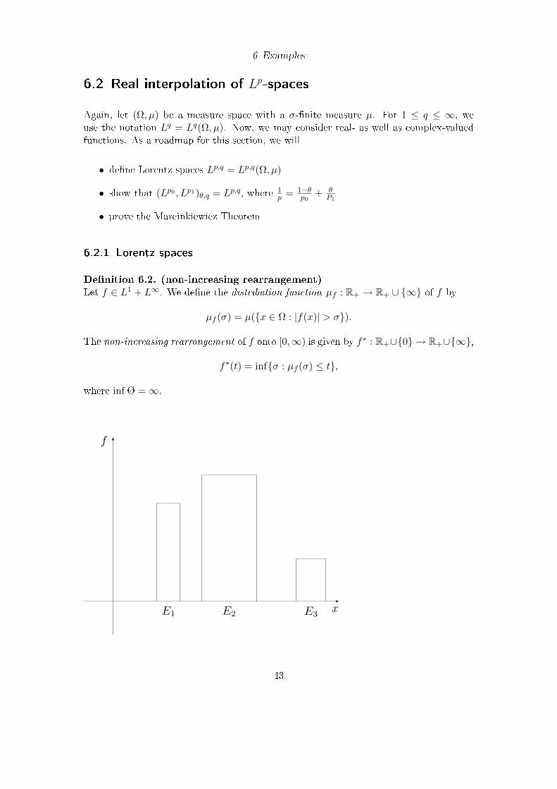
Denition 6.2. (non-increasing rearrangement)Let f ∈ L1 + L∞. We dene the distribution function µf : R+ → R+ ∪ ∞ of f by
µf (σ) = µ(x ∈ Ω : |f(x)| > σ).
The non-increasing rearrangement of f onto [0,∞) is given by f∗ : R+∪0 → R+∪∞,
f∗(t) = infσ : µf (σ) ≤ t,
where inf Ø = ∞.
43
6 Examples
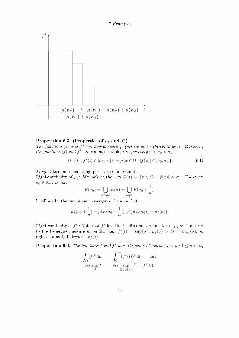
Proposition 6.3. (Properties of µf and f∗)The functions µf and f∗ are non-increasing, positive and right-continuous. Moreover,
the functions |f | and f∗ are equimeasurable, i.e. for every 0 < σ0 < σ1,
|t > 0 : f∗(t) ∈ [σ0, σ1]| = µx ∈ Ω : |f(x)| ∈ [σ0, σ1]. (6.1)
Proof. Clear: non-increasing, positive, equimeasurable.Right-continuity of µf : We look at the sets E(σ) = x ∈ Ω : |f(x)| > σ. For everyσ0 ∈ R+, we have
E(σ0) =⋃σ>σ0
E(σ) =⋃n∈N
E(σ0 +1n
).
It follows by the monotone convergence theorem that
µf (σ0 +1n
) = µ(E(σ0 +1n
)) µ(E(σ0)) = µf (σ0).
Right-continuity of f∗ : Note that f∗ itself is the distribution function of µf with respectto the Lebesgue measure m on R+, i.e. f∗(t) = supσ : µf (σ) > t = mµf
(σ), soright-continuity follows as for µf .
Proposition 6.4. The functions f and f∗ have the same Lp-norms, i.e. for 1 ≤ p <∞,Ω|f |p dµ =
∞
0(f∗(t))p dt and
ess supΩf = ess sup
R+∪0f∗ = f∗(0).
44
6 Examples
Proof. Exercise.
Denition 6.5. (Lorentz spaces)For 1 ≤ p, q ≤ ∞, we dene the Lorentz spaces by
Lp,q(Ω, µ) :=
f ∈ L1 + L∞ : ‖f‖Lp,q =
( ∞
0(t1/pf∗(t))q
dtt
)1/q
<∞
for q <∞ and by
Lp,∞(Ω, µ) :=f ∈ L1 + L∞ : ‖f‖Lp,∞ = sup
t>0t1/pf∗(t) <∞
otherwise. The Lp,∞-spaces are also called Marcinkiewicz spaces. Note that Lp,p = Lp
by Proposition 6.4.
6.2.2 Lorentz spaces and the K-functional
Theorem 6.6. For 0 < θ < 1 and 1 ≤ q ≤ ∞, we have that
(L1, L∞)θ,q = L1
1−θ,q.
Proof. We prove the theorem in two steps:
1. We show that
K(t, f, L1, L∞) = t
0f∗(s) ds (6.2)
for all t > 0. Note that historically, the Lorentz spaces were used before thisconnection to real interpolation spaces was discovered. In the following, let t > 0and
Et = x ∈ Ω : |f(x)| > f∗(t),Dt = x ∈ Ω : |f(x)| = f∗(t),
so that µ(Et) ≤ t ≤ µ(Et ∪Dt). From (6.1) and Proposition 6.4, we get that forevery y ∈ Dt - which we need if µ(Dt) 6= 0 - ,
t
0f∗(s) ds =
Et
|f(x)|dµ+ (t− µ(Et))|f(y)|. (6.3)
Rigorously, this can be seen from the following argument. We may write
(χEtf)∗(s) = infσ : µ(x ∈ Ω : |χEt(x)| · |f(x)| > σ) ≤ s= infσ : µ(x ∈ Ω : |f(x)| > σ ∩ Et) ≤ s= infσ : µ(x ∈ Ω : |f(x)| > max(σ, f∗(t))) ≤ s. (6.4)
45
6 Examples
In the case s ≥ µ(Et), if f∗(t) > 0, we get (χEtf)∗(s) = 0, as
µ(x ∈ Ω : |f(x)| > f∗(t)) = µ(Et) ≤ s,
otherwise if f∗(t) = 0, then (χEtf)∗(s) = f∗(s). In the case s < µ(Et), we seefrom the last line in (6.4) that (χEtf)∗(s) = f∗(s). If f∗(t) = 0, then (6.3) followsbecause |f(y)| = 0. If f∗(t) 6= 0, then
t
0f∗ =
µ(Et)
0f∗ +
t
µ(Et)f∗ =
Et
|f |+ t
µ(Et)f∗
by Proposition 6.4. Moreover, we have f∗(s) = f∗(t) = |f(y)| for every s ∈[µ(Et), t] as clearly f∗(t) ≤ f∗(s) ≤ f∗(µ(Et)) and by denition,
f∗(µ(Et)) = infσ > 0 : µx : |f(x)| > σ ≤ µx : |f(x)| > |f∗(t)| ≤ f∗(t).
This gives (6.3).It follows that for a decomposition f = f1 + f∞ with f1 ∈ L1 and f∞ ∈ L∞, wehave
t
0f∗(s) ds ≤
Et
|f1|dµ+ (t− µ(Et))|f1(y)|
+ µ(Et) supx∈Et
|f∞(x)|+ (t− µ(Et))|f∞(y)|
≤ ‖f1‖L1 + t‖f∞‖L∞ .
For the other inequality, we may choose the following decomposition of f ,
f1(x) =
f(x)− f(x)
|f(x)|f∗(t) for x ∈ Et,
0 otherwise.
and
f∞ = f − f1.
First, we show that
‖f1‖L1 = µ(Et)
0f∗(s)− f∗(t) ds.
This follows from Proposition 6.4 if f∗(t) = 0. Otherwise,
‖f1‖L1 =
Ω|χEtf1| =
µ(Et)
0f∗1 (s) ds
by (6.4). On Et, we have f1 = (|f | − f∗(t))ei arg f , so that
|f1| = (|f | − f∗(t))χEt .
46
6 Examples
Since |f1|∗ = f∗1 , we get
f∗1 = infσ : µ(x : χEt(|f | − f∗(t))) ≤ s= infσ : µ(x ∈ Et : |f | > σ + f∗(t)) ≤ s
|f |>f∗(t) only on Et= infσ : µ(x : |f | > σ + f∗(t)) ≤ s= infσ > f∗(t) : µ(x : |f | > σ) ≤ s − f∗(t). (6.5)
Now if σ ≤ f∗(t), then
µ(x : |f | > σ) ≥ µ(x : |f | > f∗(t)) = µ(Et) > s,
so that from (6.5) we see that
f∗1 (s) = infσ : µ(x : |f | > σ) ≤ s − f∗(t) = f∗(s)− f∗(t).
It follows that
‖f1‖L1 = µ(Et)
0f∗(s)− f∗(t) ds ≤
t
0f∗(s) ds− tf∗(t)
and that|f∞(x)| ≤ |f∗(t)χEt(x)‖ ≤ f∗(t), x ∈ Ω,
so that
K(t, f, L1, L∞) ≤ ‖f1‖L1 + t‖f∞‖L∞ = t
0f∗(s) ds.
2. From (6.2), the claim follows fairly directly. Note that t0 f
∗(s) ds ≥ tf∗(t), as f∗
is non-increasing, so that for q <∞, we have
‖f‖(L1,L∞)θ,q =[ ∞
0t−θqKq(t, f)
dtt
]1/q
≥[ ∞
0t(1−θ)q(f∗(t))q
dtt
]1/q
= ‖f‖L
11−θ
,q ,
and for q = ∞,
supt>0
|t−θK(t, f)| ≥ supt>0
|t1−θf∗(t)| = ‖f‖L
11−θ
,∞ .
On the other hand, by the Hardy-Young inequality, Lemma 3.2, we have
‖t−θK(t, f)‖qLq∗
= ∞
0t−θq
( t
0sf∗(s)
dss
)q dtt
≤ 1θq
∞
0s(1−θ)q(f∗(s))q
dss
=1θq‖f‖q
L1
1−θ,q
47
6 Examples
and also
supt>0
|t−θK(t, f)| ≤ t−θ( t
0
dss1−θ
)sups>0
(s1−θf∗(s)) =1θ‖f‖
L1
1−θ,∞ .
Theorem 6.7. For 1 < p0 < p1 <∞, 0 < θ < 1 and 1 ≤ q ≤ ∞ we have
(Lp0 , Lp1 )θ,q = Lp,q, where1p
=1− θ
p0+
θ
p1.
In particular, if p0 < q < p1 and θ = p1q
(p0−qp0−p1
), then
(Lp0 , Lp1)θ,q = Lq.
Moreover, for 1 < p0 < p1 <∞, 0 < θ < 1 and 1 ≤ q0 ≤ q1 ≤ ∞, we have
(Lp0,q0 , Lp1,q1)θ,q = Lp,q
for p as above.
Proof. By Theorem 6.6, we know that Lp = (L1, L∞)1−1/p,p, so Lp ∈ J1−1/p∩K1−1/p(L1, L∞).
We can therefore apply the Reiteration Theorem 4.4 to get
(Lp0 , Lp1)θ,q = (L1, L∞)ω,q,
where ω = (1− θ)(1− 1/p0) + θ(1− 1/p1). By Theorem 6.6, (L1, L∞)ω,q = Lp,q, where1p = 1− ω = 1−θ
p0+ θ
p1. The same argument yields the third statement.
6.2.3 The Marcinkiewicz Theorem
Denition 6.8. Let (Ω, µ) and (Λ, ν) be two σ-nite measure spaces. A linear operatorT : L1(Ω, µ) + L∞(Ω, µ) → L1(Λ, ν) + L∞(Λ, ν) is called of weak type (p, q), if there isan M > 0 such that
supσ>0
σ(νy ∈ Λ : |Tf(y)| > σ)1/q = supt>0
t1/q(Tf)∗(t) ≤M‖f‖Lp(Ω,µ).
for all f ∈ Lp(Ω, µ), i.e. the restriction of T to Lp(Ω, µ) is bounded from Lp(Ω, µ) toLq,∞(Λ, ν).T is said to be of strong type (p, q) if its restriction to Lp(Ω, µ) is bounded from Lp(Ω, µ)to Lq(Λ, ν).
Clearly, every operator of strong type (p, q) is also of weak type (p, q).
48
6 Examples
Theorem 6.9. Let T : L1(Ω, µ)+L∞(Ω, µ) → L1(Λ, ν)+L∞(Λ, ν) be of weak type (p0, q0)and (p1, q1) with constants M0,M1, respectively and 1 < p0, p1 < ∞, 1 < q0, q1 < ∞,
q0 6= q1 and p0 ≤ q0, p1 ≤ q1. For 0 < θ < 1 let
1p
=1− θ
p0+
θ
p1,
1q
=1− θ
q0+θ
q1.
Then T is of strong type (p, q) and there is a constant C, independent of θ, such that
‖Tf‖Lq(Λ,ν) ≤ CM1−θ0 M θ
1 ‖f‖Lp(Ω,µ)
for all f ∈ Lp(Ω, µ).
Proof. For i = 0, 1 , T is bounded from Lpi(Ω, µ) to Lqi,∞(Λ, ν) with norm Mi. Sincereal interpolation is exact of type θ, Theorem 2.4, it follows that
‖T‖L((Lp0 ,Lp1 )θ,p,(Lq0,∞,Lq1,∞)θ,p) ≤M1−θ
0 M θ1 .
By Theorem 6.7, (Lp0 , Lp1)θ,p = Lp,p = Lp(Ω, µ) and (Lq0,∞, Lq1,∞)θ,p = Lq,p(Λ, ν).Since pi ≤ qi, also p ≤ q, so that Lq,p → Lq,q = Lq(Λ, ν) by Theorem 2.5. This yieldsthe claim.
6.3 Hölder spaces
Reminder: f ∈ C1(Ω) ⇔ f : Ω ⊂ Rn → R is continuously dierentiable and ‖f‖C1(Ω) :=‖f‖∞ +
∑ni=1 ‖Dif‖∞ <∞.
Denition 6.10. For θ ∈ (0, 1), we dene the Hölder space Cθ(Ω) for every open setΩ ⊂ Rn, n ∈ N, as the space of bounded and uniformly θ-Hölder continuous functions fwith the norm
‖f‖Cθ(Ω) = ‖f‖∞ + [f ]Cθ = ‖f‖∞ + supx,y∈Ω,x 6=y
|f(x)− f(y)||x− y|θ
.
Theorem 6.11. For θ ∈ (0, 1), we have that
(C(Rn), C1(Rn))θ,∞ = Cθ(Rn)
with equivalence of norms.
Proof. For convenience, we may write C,C1 etc. in the following. First we show that(C,C1)θ,∞ → Cθ: Clearly, for every f ∈ C1, ‖f‖∞ ≤ ‖f‖C1 . For every decompositionf = f0 + f1, f0 ∈ C, f1 ∈ C1, we have ‖f‖∞ ≤ ‖f0‖∞ + ‖f1‖∞, so
‖f‖∞ ≤ K(1, f, C,C1) ≤ ‖f‖(C,C1)θ,∞ .
49
6 Examples
Moreover, if x 6= y, we have that
|f(x)− f(y)| ≤ |f0(x)− f0(y)|+ |f1(x)− f1(y)| ≤ 2‖f0‖∞ + ‖f1‖C1 |x− y|.
Taking the inmum over these decompositions gives
|f(x)− f(y)| ≤ 2K(|x− y|, f, C,C1) ≤ 2|x− y|θ‖f‖(C,C1)θ,∞
by (2.2), so that f must be θ-Hölder continuous and ‖f‖Cθ = ‖f‖∞+[f ]θ ≤ 3‖f‖(C,C1)θ,∞ .
Now we show that Cθ → (C,C1)θ,∞: Let f ∈ Cθ. We want to decompose f into a C-and a C1-part with good estimates. Let ϕ ∈ C∞ such that ϕ ≥ 0, suppϕ ⊂ B1 and‖ϕ‖L1 = 1. For every t > 0, we consider
f1,t(x) =1tn
Rn
f(y)ϕ(x− y
t) dy,
f0,t(x) = f(x)− f1,t(x). (6.6)
It follows that f0,t(x) = 1tn
Rn(f(x)− f(x− z))ϕ( zt ) dz, so
‖f0,t‖∞ ≤ [f ]Cθ
1tn
Rn
|y|θϕ(y
t) dy = tθ[f ]Cθ
Rn
|w|θϕ(w) dw.
It also follows that ‖f1,t‖∞ ≤ ‖f‖∞. It remains to look at the derivatives, for i = 1, . . . , n,
Dif1,t(x) =1
tn+1
Rn
f(y)(Diϕ)(x− y
t) dy.
Since ϕ has compact support, we have
Rn Diϕ(x−yt ) dy = 0. We get that
Dif1,t(x) =1
tn+1
Rn
(f(x− z)− f(x))(Diϕ)(z
t) dz, (6.7)
so that
‖Dif1,t‖∞ ≤ 1tn+1
Rn
|f(x− z)− f(x)||z|θ
|z|θ(Diϕ)(z
t) dz
= tθ−1[f ]Cθ
Rn
|w|θ(Diϕ)(w) dw.
For 0 < t ≤ 1, it follows that
t−θK(t, f) ≤ t−θ(‖f0,t‖∞ + t‖f1,t‖C1) ≤ C‖f‖Cθ .
For t > 1 , we set f0,t = f and f1,t = 0 to immediately get that
t−θK(t, f) ≤ t−θ‖f‖∞ ≤ ‖f‖∞.
It follows that f ∈ (C,C1)θ,∞ and that ‖f‖(C,C1)θ,∞ ≤ C‖f‖Cθ , with C depending onlyon the choice of ϕ.
50
6 Examples
Remark 6.12. The following results are mostly taken from [4], Chapter 2: 1. followsimmediately, 2., 3., 4, could also be an exercise:
1. By Reiteration, Theorem 4.4:
(Cα, Cβ)θ,∞ = ((C,C1)α,∞, (C,C1)β,∞)θ,∞ = (C,C1)ω,∞ = Cω,
where α, β ∈ (0, 1) and ω = (1− θ)α+ θβ.
2. It holds that
”(C,C1)1,∞” = Lip(Rn),
where Lip(Rn) is the space of Lipschitz continuous and bounded functions,
‖f‖Lip(Rn) = ‖f‖∞ + supx 6=y
|f(x)− f(y)||x− y|
.
3. C1 is not dense in Cθ.
4. For any interval I ⊂ R, X a Banach space, 0 < θ < 1,
(C(I;X), C1(I,X))θ,∞ = Cθ(I;X).
5. Let m ∈ N and θ ∈ (0, 1). If θm is not an integer,
(C,Cm)θ,∞ = Cθm.
6. In the situation of 3., if θm = 1, then
(C,Cm)θ,∞ = C1,
where for every 0 < α < 2, Cα is given by
Cα = f ∈ C : [f ]Cα = supx 6=y
|f(x)− 2f(x+y2 ) + f(y)||x− y|α
<∞,
‖f‖Cα = ‖f‖∞ + [f ]Cα .
For α 6= 1, these spaces are equivalent to the Cα's.
6.4 Slobodeckii spaces
Dilemma I: How to dene Wα,p(Rn) for α /∈ N, 1 ≤ p <∞ and n ∈ N?
1. Wα,p = (Lp,W 1,p)α,p for 0 < α < 1.
51
6 Examples
2. Wα,p is the set of functions f ∈ Lp, such that
[f ]α,p =(
Rn×Rn
|f(x)− f(y)|p
|x− y|αp+ndxdy
)1/p
<∞,
endowed with the norm ‖f‖Wα,p = ‖f‖Lp + [f ]Wα,p .
Theorem 6.13. The two denitions above coincide.
Dilemma II: How to dene Wα,p(Ω) for open sets Ω ⊂ Rn?
1. as in 1. above.
2. Wα,p(Ω) is the space of functions which are restrictions of functions in Wα,p(Rn)to Ω.
Theorem 6.14. The two denitions above coincide if Ω is a domain with uniformly
C1-boundary.
Denition 6.15. On an open set Ω ⊂ Rn, for α ∈ (0, 1), the (Sobolev-)Slobodeckii spacesWαp (Ω) are dened by
Wαp (Ω) = (Lp(Ω),W 1,p(Ω))α,p.
Proof. of Theorem 6.13. It works similarly as the proof for Hölder spaces, Theorem 6.11.First we show that Wα
p →Wα,p, dened as in 2.:
Note that for every f1 ∈W 1,p and h ∈ Rn\0, we have that (exercise)(Rn
(|f1(x+ h)− f1(x)|
|h|
)pdx)1/p
≤ ‖|Df1|‖Lp .
For all f ∈ (Lp,W 1,p)α,p and h ∈ Rn, we set f0,h ∈ Lp and f1,h ∈ W 1,p such thatf = f0,h + f1,h and
‖f0,h‖Lp + |h|‖f1,h‖W 1,p ≤ 2K(|h|, f).
Moreover,
|f(x+ h)− f(x)|p
|h|αp+n≤ 2p−1
(|f0,h(x+ h)− f0,h(x)|p
|h|αp+n+|f1,h(x+ h)− f1,h(x)|p
|h|αp+n
)and so
Rn
|f(x+ h)− f(x)|p
|h|αp+ndx ≤ 2p−1
Rn
(|f0,h(x+ h)− f0,h(x)|p
|h|αp+n+|f1,h(x+ h)− f1,h(x)|p
|h|αp+n
)dx
≤ 2p‖f0,h‖pLp
|h|αp+n+ 2p−1 |h|p‖|Df1,h|‖pLp
|h|αp+n
≤ Cp|h|−αp−n(‖f0,h‖Lp + |h|‖f1,h‖W 1,p)p
≤ Cp|h|−αp−nK(|h|, f)p.
52
6 Examples
Therefore,
[f ]pα,p =
Rn×Rn
|f(x+ h)− f(x)|p
|h|αp+ndxdh
≤ Cp
Rn
|h|−αp−nK(|h|, f)p dh
= Cp,n
∞
0
K(r, f)p
rαp+1dr
= Cp,n‖f‖p(Lp,W 1,p)α,p.
From the embedding (Lp,W 1,p)α,p → Lp + W 1,p = Lp we also get that ‖f‖Lp ≤C‖f‖(Lp,W 1,p)α,p
, so that in conclusion,
‖f‖Wα,p ≤ C‖f‖(Lp,W 1,p)α,p.
We now check the other embedding: For every f ∈ Wα,p, we dene f0,t and f1,t as in(6.6). It follows that
‖f0,t‖pLp =
Rn
(Rn
|f(x)− f(y)| 1tnϕ(x− y
t) dy
)pdx
≤
Rn×Rn
|f(x)− f(y)|p 1tnϕ(x− y
t) dy dx
from the Hölder inequality applied to
|f(x)− f(y)|(t−nϕ(x− y
t))1/p · (t−nϕ(
x− y
t))1−1/p.
We get that
∞
0t−αp‖f0,t‖pLp
dtt≤
∞
0
(Rn×Rn
t−αp|f(x)− f(y)|p 1tnϕ(x− y
t) dy dx
)dtt
=
Rn×Rn
|f(x)− f(y)|p( ∞
0t−αp
1tnϕ(x− y
t)dtt
)dy dx
=
Rn×Rn
|f(x)− f(y)|p( ∞
|x−y|t−αp
1tnϕ(x− y
t)dtt
)dy dx
≤ ‖ϕ‖∞αp+ n
Rn×Rn
|f(x)− f(y)|p
|x− y|αp+ndy dx
= C[f ]pα,p.
By using (6.7), we get that
∞
0t(1-α)p‖Dif1,t‖pLp
dtt≤Cp−1i ‖Diϕ‖∞αp+ n
[f ]pα,p,
53
6 Examples
where Ci =
Rn |Diϕ(y)|dy. We also see directly that ‖f1,t‖Lp ≤ ‖f‖Lp‖ϕ‖L1 = ‖f‖Lp ,so 1
0t(1−α)p‖f1,t‖pLp
dtt≤ 1
(1− α)p‖f‖pLp .
It follows that
t−αK(t, f, Lp,W 1,p) ≤ t−α‖f0,t‖Lp + t1−α‖f1,t‖W 1,p ∈ Lp∗(0, 1)
and that its norm is estimated by C‖f‖Wα,p . Again, this suces to get that f ∈(Lp,W 1,p)α,p.
6.5 Functions on domains
This section follows parts of Chapters 3,4 and 5 in [1], in particular, pages 147-152.
Denition 6.16. A domain Ω ⊂ Rn satises the uniform Cm-regularity condition ifthere exists a locally nite open cover Uj of ∂Ω and a corresponding sequence Φj ofm-Dieomorphisms taking Uj onto the unit ball B1(0) with inverses Ψj = Φ−1
j such that
1. for some nite R, every intersection of R+ 1 of the sets Uj is empty,
2. for some δ > 0,
Ωδ = x ∈ Ω : dist(x, ∂Ω) < δ ⊂ ∪jΨj(B1/2(0)),
3. for each j, Φj(Uj ∩ Ω) = y ∈ B1(0) : yn > 0,
4. there is a nite constant M > 0, such that for every j, ‖Φj‖Cm(Uj) ≤ M and‖Ψj‖Cm(B1(0)) ≤M .
Proof. Of Theorem 6.14. We use that for every uniform C1-domain Ω, there is anextension operator E, such that
E ∈ L(Lp(Ω), Lp(Rn)), E ∈ L(W 1,p(Ω),W 1,p(Rn)), (6.8)
and E ∈ L(Wα,p(Ω),Wα,p(Rn)). Here,Wα,p(Rn) is given as in Dilemma I.2 andWα,p(Ω)is given as the space of functions which are restrictions of functions in Wα,p(Rn) to Ω.This operator can be constructed similarly as before, rst for the half-space, then bylocalization. However, in order to get that E ∈ L(Wα,p(Ω),Wα,p(Rn)), we take functionsfrom W 1,p(Rn
+) and extend by exact reection, not as in the proof of Theorem 6.19 forcontinuously dierentiable functions.
From (6.8), it follows that E ∈ L(Wαp (Ω),Wα
p (Rn)) as real interpolation is exact oftype θ. For every f ∈ Wα,p(Ω), we have that Ef ∈ Wα,p(Rn) = Wα
p (Rn). Moreover,the restriction operator R : f ∈ Lp(Rn) 7→ f |Ω clearly belongs to L(Lp(Rn), Lp(Ω)) ∩
54
6 Examples
L(W 1,p(Rn),W 1,p(Ω)) and thus to L(Wαp (Rn),Wα
p (Ω)). It follows that R(E(f)) belongsto Wα
p (Ω) and we have the estimate
‖f‖Wαp (Ω) ≤ CE‖E(f)‖Wα
p (Rn) ≤ CE,α,p‖E(f)‖Wα,p(Rn) ≤ C‖f‖Wα,p(Ω).
On the other hand, for f ∈Wαp (Ω), we know that Ef ∈Wα,p(Rn) and so R(Ef) = f ∈
Wα,p(Ω) and‖f‖Wα,p(Ω) ≤ ‖E(f)‖Wα
p (Rn) ≤ ‖f‖Wαp (Ω).
Remark. In the same way, we get that for Ω ⊂ Rn with a uniformly C1-boundary,
(C(Ω), C1(Ω))θ,∞ = Cθ(Ω).
55
7 Function Spaces from Fourier Analysis
Reminder I:
• S(Rn) Schwartz space, S ′(Rn) the dual space of S(Rn)
• Fourier transform:
(Fϕ)(ξ) = ϕ(ξ) =1
(2π)n/2
Rn
e−i(x·ξ)ϕ(x) dx,
and F ,F−1 : S(Rn) → S(Rn), S ′(Rn) → S ′(Rn), F ∈ L(L2(Rn)) unitary, F :Lp → Lp
′if 1 ≤ p ≤ 2.
• Dα(Fϕ)(ξ) = (−i)|α|F(xαϕ(x)) and ξα(Fϕ)(ξ) = (−i)|α|F(Dαϕ(x)).
Denition 7.1. (Bessel potential spaces)Let 1 < p <∞ and s ∈ R, we dene
Hs,p(Rn) :=f ∈ S ′(Rn) : ‖f‖Hs,p(Rn) := ‖F−1(1 + |ξ|2)
s2Ff‖Lp(Rn) <∞
.
Remark 7.2. Hopefully, we will be able to show that Hθm,p = [Lp,Wm,p]θ.
Reminder II: Sobolev spaces: 1 ≤ p ≤ ∞, k ∈ N,
W k,p(Rn) :=
f ∈ Lp(Rn) : ‖f‖Wk,p(Rn) :=∑|α|≤k
‖Dαf‖Lp(Rn) <∞
.
Question: If 1 < p <∞, k ∈ N, then Hk,p(Rn) = W k,p(Rn)?
1. k = 0: Lp(Rn) = H0,p(Rn) = W 0,p(Rn)
2. p = 2: true, using Plancherel
3. p 6= 2: also true, using Mikhlin multiplier theorem
We immediately see 1., we look at 2. and 3. in the following.
Note that for any multi-index |α| ≤ k and ξ ∈ Rn,
|ξα| ≤ |ξ||α| ≤ (1 + |ξ|2)k2 (7.1)
56
7 Function Spaces from Fourier Analysis
and that for every f ∈ Hk,2, we automatically have f ∈ L2. It follows that
‖f‖Wk,2 ≤∑|α|≤k
‖FDαf‖L2 ≤∑|α|≤k
‖ξαFf‖L2 ≤ C‖F−1(1 + |ξ|2)k2Ff‖L2 = C‖f‖Hk,2 .
(7.2)Conversely, let ρ : R → [0, 1], ρ ∈ C∞(R) and ρ(s) = −ρ(−s) such that
ρ(t) =
0,1,
t ≤ 12
t ≥ 0, so that
(1 + |ξ|2)k2
1 +∑n
i=1 ρk(ξi)ξki
→ 1|ξ|→0,∞
.
It follows that
(1 + |ξ|2)k2 ≤ Cn,k
(1 +
n∑i=1
ρk(ξi)ξki
). (7.3)
We get that
‖f‖Hk,2 = ‖(1 + |ξ|2)k2Ff(ξ)‖L2
= ‖ (1 + |ξ|2)k2
1 +∑n
i=1 ρk(ξi)ξki
(1 +
n∑i=1
ρk(ξi)ξki
)Ff(ξ)‖L2
≤ Cn,k
(‖Ff‖L2 +
n∑i=1
‖ρk(ξi)ξki Ff(ξ)‖L2
)
≤ Cn,k
(‖Ff‖L2 +
n∑i=1
‖(−i)kF(∂k
∂ixkf)(x)‖L2
)≤ C‖f‖Wk,2 .
Now we look at the case p 6= 2 and introduce a preliminary concept, without proofs.
Denition 7.3. Let 1 ≤ p ≤ ∞ and m ∈ L∞(Rn; C). Then m is called a Fourier
multiplier, m ∈ Mp, if there is a constant c > 0, such that for all f ∈ S(Rn),
‖F−1mFf‖Lp ≤ c‖f‖Lp ,
so that the operator
Tm : S(Rn) → C0(Rn), f 7→ F−1mFf
can be extended to a bounded operator on Lp.
Theorem 7.4. (Mikhlin-Hörmander)
Let 1 < p < ∞. Then m ∈ Cbn2 c+1(Rn\0) is a Fourier multiplier in Mp if there is a
constant cm > 0 such that
|ξ||β||Dβm(ξ)| ≤ cm
for all ξ ∈ Rn\0 and multi-indices |β| ≤⌊n2
⌋+ 1.
57
7 Function Spaces from Fourier Analysis
Proof. For example, [3], Theorem 6.1.6 for a proof and a more general version of thetheorem.
Theorem 7.5. Let 1 < p < ∞, k ∈ N0, s ∈ R. Then Hs,p(Rn) is a Banach space and
we have
W k,p(Rn) = Hk,p(Rn).
Proof. The idea is as in the case p = 2, only we use Theorem 7.4, too. We know that
‖f‖Wk,p =∑|α|≤k
‖Dα(F−1Ff)‖Lp =∑|α|≤k
‖F−1(ξαFf(ξ))‖Lp .
It follows that ‖f‖Wk,p ≤ C‖f‖Hk,p , if we can show that
‖F−1(ξαFf(ξ))‖Lp ≤ Cn,k‖F−1(1 + |ξ|2)k2Ff‖Lp
for all α. We dene
mα,k(ξ) =ξα
(1 + |ξ|2)k2
for |α| ≤ k and show that it is a Fourier multiplier. For |α| = 0, we have |mα,k(ξ)| ≤ 1by (7.1). If |α| = 1, we get
|ξ|∣∣∣∣ ∂∂ξj ξα
(1 + |ξ|2)k/2
∣∣∣∣ = |ξ|
∣∣∣∣∣αjξα11 · · · · · ξαj−1
j · · · · · ξαnn (1 + |ξ|2)k/2 − ξjk(1 + |ξ|2)k/2−1
(1 + |ξ|2)k
∣∣∣∣∣=
|ξ|(1 + |ξ|2)k/2
∣∣∣∣αj − ξjk
(1 + |ξ|2)
∣∣∣∣ ≤ 2k.
By more similar calculations and induction, the claim can be proved. It follows that
‖F−1ξαFf‖Lp = ‖F−1mα,k(1 + |ξ|2)k/2Ff‖Lp
= ‖F−1mα,kFF−1(1 + |ξ|2)k/2Ff‖Lp
≤ Cn,k‖F−1(1 + |ξ|2)k/2Ff‖Lp
for every f ∈ Lp.For the converse estimate, we dene
mρ,k(ξ) =(1 + |ξ|2)k/2
1 +∑n
i=1 ρk(ξi)ξki
and show that it is a Fourier multiplier. For |α| = 0, we have |mρ,k(ξ)| ≤ Cn,k by (7.3).For |α| = 1, we use the notation 1 +
∑ni=1 ρ
k(ξi)ξki =: ρ, (1 + |ξ|2) =: Mξ and calculate:
|ξ|∣∣∣∣ ∂∂ξj mρ,k(ξ)
∣∣∣∣ = |ξ|
∣∣∣∣∣∣ξjkMk/2−1ξ ρ−M
k/2ξ [kρk−1(ξj)ρ′(ξj)ξkj + ρk(ξj)kξk−1
j ]
ρ2
∣∣∣∣∣∣≤ Cn,k|ξ|
Mk/2−1ξ
ρ2k∣∣∣M (k+1)/2
ξ −Mξ
(Ck +M
(k−1)/2ξ
)∣∣∣≤ Cn,kM
1/2ξ
Mk/2−1ξ
ρ2M
k/2+1/2ξ ≤ Cn,km
2ρ,k(ξ) ≤ Cn,k.
58
7 Function Spaces from Fourier Analysis
Again, we could calculate similarly for |α| > 1 and use induction to get the claim. Wenow use that ξ 7→ ρk(ξj)(−i)k is a Fourier multiplier for every 1 ≤ j ≤ n, to get that
‖f‖Hk,p ≤ ‖F−1mρ,kρkFf‖Lp ≤ Cm‖F−1ρkFf‖Lp
≤ C(‖f‖Lp + ‖F−1(n∑i=1
ρk(ξi)ξki )Ff‖Lp)
= C(‖f‖Lp + ‖F−1(n∑i=1
ρk(ξi)(−i)kF(∂ki f))‖Lp)
≤ C(‖f‖Lp +n∑i=1
‖∂ki f‖Lp) ≤ C‖f‖Wk,p .
We will come back to Bessel potential spaces, but now want to dene and consider Besovspaces.
Denition 7.6. A sequence of functions (ϕj)j∈N ⊂ C∞c (Rn) is called dyadic partition of
unity, if and only if
1. suppϕj ⊂ Aj , j ∈ N, where
A0 = B2(0),Aj = x ∈ Rn : 2j−1 < |x| < 2j+1, j 6= 0,
2.∑∞
j=0 ϕj(x) = 1,
3. for all multi-indices γ = (γ1, ..., γn) ∈ Nn0 , there is a constant cγ , such that
2j|γ||Dγϕj(x)| ≤ cγ .
Example: If ϕ ∈ S(Rn), suppϕ ⊂ B2(0) and ϕ(x) = 1 for |x| ≤ 1, then setting ϕ0 = ϕand ϕj(x) = ϕ(2−jx)− ϕ(2−j+1x) for j 6= 0 yields a dyadic partition of unity.
Denition 7.7. (Besov spaces)Let s ∈ R, 1 ≤ p, q ≤ ∞ and (ϕj)j∈N a dyadic partion of unity. Then the Besov spacesBsp,q(Rn) are the spaces of all functions f ∈ S ′(Rn) such that
‖f‖Bsp,q(Rn) :=
(∑∞
j=0 2jsq‖F−1ϕiFf‖qLp(Rn)
)1/q, q <∞
supj∈N02js‖F−1ϕFf‖Lp(Rn), q = ∞
<∞.
Remark 7.8. We will show that (Lp,Wm,p)θ,q = Bθmp,q , so that in particular, Bs
p,p = W sp .
Proposition 7.9. Bsp,q(Rn) is a Banach space and choosing two dierent dyadic parti-
tions yields equivalent norms.
59
7 Function Spaces from Fourier Analysis
Proof. Exercise.
In order to get interpolation results for Besov spaces, we start from the following type ofspaces.
Denition 7.10. Let X be a Banach space, σ ∈ R and 1 ≤ p ≤ ∞. Then lσp (X) is thespace of sequences (xj)j∈N ⊂ X such that
‖x‖lσp (X) :=
(∑∞
j=0 2jσp‖xj‖pX)1/p
, p <∞supj∈N0
2jσ‖xj‖X , p = ∞<∞.
Remark 7.11. It is a Banach space. If X = C and σ = 0, then lσp (X) = lp. Moreover, if1 ≤ r ≤ p ≤ ∞, then lσr → lσp .
Proof. Exercise.
Theorem 7.12. Let X be a Banach space, s0, s1 ∈ R, s0 6= s1, 1 ≤ p0, p1, p ≤ ∞ and
0 < θ < 1. Then we get
(ls0p0(X), ls1p1(X))θ,p = lsp(X),
where s = (1− θ)s0 + θs1.
Proof. Use Theorem 2.5.6 and show that
(ls0∞, ls1∞)θ,p → lsp → (ls01 , l
s11 )θ,p (7.4)
to get that
lsp → (ls01 , ls11 )θ,p → (ls0p0 , l
s1p1)θ,p → (ls0∞, l
s1∞)θ,p → lsp.
We now rst show the rst embedding in (7.4). We know that
K(t, x, ls0∞, ls1∞) = inf
x=x0+x1(supj
2js0‖x0j‖X + t sup
j2js1‖x1
j‖X)
for all x ∈ ls0∞ + ls1∞ = lmin(s0,s1)∞ . We look at
x0j =
xj, 2js0 ≤ t2js1 ,0, otherwise.
and x1 = x− x0,
to see that
K(t, x, ls0∞, ls1∞) ≤ 2 sup
jmin(2js0 , t2js1)‖xj‖X .
On the other hand, clearly,
supj
min(2js0 , t2js1)‖xj‖ ≤ supj
(2js0‖x0j‖X + t2js1‖x1
j‖X)
60
7 Function Spaces from Fourier Analysis
for all decompositions x = x0 + x1, so that
K(t, x, ls0∞, ls1∞) ∼ sup
jmin(2js0 , t2js1)‖xj‖X .
Wlog, we assume that s0 > s1, since we could consider (ls1p1 , ls0p0)1−θ,q instead. We treat the
case when p < ∞ and use the decomposition (0,∞) = ∪∞k=−∞[2(k−1)(s0−s1), 2k(s0−s1)).For x ∈ (ls0∞, l
s1∞)θ,p,
‖x‖p(l
s0∞ ,ls1∞)θ,p
=∞∑
k=−∞
2k(s0−s1)
2(k−1)(s0−s1)t−θpK(t, x, ls0∞(X), ls1∞(X))p
dtt
≥∞∑
k=−∞2−θpk(s0−s1) sup
jmin(2js0p, 2kp(s0−s1)2js1p)‖xj‖pX
2k(s0−s1)
2(k−1)(s0−s1)
dtt
≥ C
∞∑k=−∞
2−θpk(s0−s1) min(2ks0p, 2kp(s0−s1)2ks1p)‖xk‖pX(s0 − s1) ln(2)
= C
∞∑k=0
2kps‖xk‖pX = C‖x‖plsp
The case p = ∞ follows analogously.Now we show the second embedding in (7.4). Again, we may assume that s0 > s1.Analogously to the l∞-situation, we see that
K(t, x, ls01 , ls11 ) ∼
∞∑j=0
min(2js0 , t2js1)‖xj‖X .
For p <∞ and x ∈ lsp, we calculate
‖x‖p(l
s01 ,l
s11 )θ,p
≤∞∑
k=−∞
2k(s0−s1)
2(k−1)(s0−s1)2−θp(k−1)(s0−s1)
∞∑j=0
min(2js0 , 2k(s0−s1)+js1)‖xj‖X
p dtt
≤ C2θp(s0−s1)∞∑
k=−∞2kps
∞∑j=0
min(2(j−k)s0 , 2(j−k)s1)‖xj‖X
p
= C
∞∑k=−∞
2kps
k∑j=−∞
2(j−k)s0‖xj‖X +∞∑
j=k+1
2(j−k)s1‖xj‖X
p .
61
7 Function Spaces from Fourier Analysis
For every t0, t1 such that s0 > t0 > s > t1 > s1, we have
k∑j=−∞
2(j−k)s0‖xj‖X ≤ 2−ks0
k∑j=−∞
2j(s0−t0)p′
1/p′ k∑j=−∞
2jt0p‖xj‖pX
1/p
≤ C2−kt0
k∑j=−∞
2jt0p‖xj‖pX
1/p
,
∞∑j=k+1
2(j−k)s1‖xj‖X ≤ 2−ks1
∞∑j=k+1
2j(s1−t1)p′
1/p′ ∞∑j=k+1
2jt1p‖xj‖pX
1/p
≤ C2−kt1
∞∑j=k+1
2jt1p‖xj‖pX
1/p
,
so that
‖x‖p(l
s01 ,l
s11 )θ,p
≤ C
∞∑k=−∞
2kps
2−kt0pk∑
j=−∞2jt0p‖xj‖pX + 2−kt1p
∞∑j=k+1
2jt1p‖xj‖pX
≤ C
∞∑j=−∞
2jsp‖xj‖pX = C‖x‖plsp .
This proves the theorem.
We now summarize several results on real and complex interpolation of Besov and Besselpotential spaces in the following theorem, and then set out to give a proof for the realpart, 1.-4. and some arguments for the complex part, 5. and 6.
Theorem 7.13. Let 0 < θ < 1, s, s0 6= s1 ∈ R, 1 ≤ p, p0, p1, q, q0, q1 ≤ ∞ and
sθ = (1− θ)s0 + θs1,1pθ
=1− θ
p0+
θ
p1,
1qθ
=1− θ
q0+θ
q1.
Then we get
1. (Bs0p,q0 , B
s1p,q1)θ,q = Bsθ
p,q,
2. (Bs0p0,q0 , B
s1p1,q1)θ,pθ
= Bsθpθ,qθ
, pθ = qθ,q0, q1 6= 1
3. (Hs0,p,Hs1,p)θ,q = Bsθp,q, 1 < p <∞,
4. (Hs,p0 ,Hs,p1)θ,pθ= Hs,pθ , 1 < p0, p1 <∞,
5. [Bs0p0,q0 , B
s1p1,q1 ]θ = Bsθ
pθ,qθ,
62
7 Function Spaces from Fourier Analysis
6. [Hs0,p0 ,Hs1,p1 ]θ = Hsθ,pθ , 1 < p0, p1 <∞.
Let (ψi)i be a dyadic partition of unity. To show 1., by looking at the map
Sψ : Bsp,q → lsq(L
p), f 7→ (F−1ψjFf)j ,
we get the idea that we can interpolate Bsp,q as the we interpolate lsq(L
p) by Theorem7.12. The following notion is helpful.
Denition 7.14. An object X in a category is called a retract of another object Y , ifthere are morphisms S : X → Y and R : Y → X in the category, such that R S = idX .In this case, the map R is called retraction, and S is called coretraction.
Clearly, the following holds true.
Lemma 7.15. If X0, X1 is a retract of Y0, Y1 in C2 with retraction R and coretrac-
tion S, then for every interpolation functor F , F(X0, X1) is a retract of F(Y0, Y1)with retraction F(R) = R and coretraction S.
Proposition 7.16. The space Bsp,q is a retract of lsq(L
p) with the coretraction S and the
retraction
Rϕ : lsq(Lp) → Bs
p,q, (xj)j 7→∞∑j=0
F−1ϕjFxj .
Proof. Clearly, Sψ ∈ L(Bsp,q, l
sq(L
p)). On the other hand,
‖Rϕ(xj)j‖Bsp,q
=
∞∑j=0
2jsq‖F−1ψjF(∞∑k=0
F−1ϕkFxj)‖qLp
1/q
≤ c
∞∑j=0
2jsq‖xj‖qLp
1/q
if we use that ψjϕj−1, ψjϕj and ψjϕj+1 are Fourier multipliers on Lp. Clearly,
RϕSψf =∞∑j=0
F−1ϕjψjFf =∞∑j=0
F−1ψjFf = f.
Theorem 7.13.1 now follows from Theorem 7.12 and Proposition 7.16.Next, we want to show 2.
Proposition 7.17. For 1 < q0, q1 ≤ ∞ and an interpolation couple X0, X1, we have
(ls0q0 (X0), ls1q1 (X1))θ,qθ = lsθqθ
((X0, X1)θ,qθ).
63
7 Function Spaces from Fourier Analysis
Proof. Unpopular but elementary exercise.
We get that by this Proposition and Theorem 6.7,
(Bs0p0,q0 , B
s1p1,q1)θ,pθ
= (ls0q0 (Lp0), ls1,q1(L
p1))θ,pθ= lsθ
qθ((Lp0 , Lp1)θ,pθ
) = lsθqθ
(Lpθ) = Bsθqθ,pθ
,
which is 2.In order to show 3., we use the following embeddings.
Proposition 7.18. For 1 < p <∞ and s ∈ R, we have
Bsp,1 → Hs,p → Bs
p,∞, (7.5)
and in particular,
B0p,1 → Lp → B0
p,∞. (7.6)
Proof. We note that (7.5) follows from (7.6) if we use that the operator Jσ = F−1(1 +|ξ|2)σ/2F is an isomorphism from Hs,p to Hs−σ,p and from Bs
p,q to Bs−θp,q . For the rst
embedding in (7.6), let f ∈ B0p,1. We can write
f =∞∑j=0
F−1ϕjFf,
to see that
‖f‖Lp ≤∞∑j=0
‖F−1ϕjFf‖Lp = ‖f‖B0p,1.
For the second embedding, let (ϕj)j as in the example above Denition 7.7. For f ∈ S,we get
F−1ϕjFf(x) = (2π)−n
Rn
eix·ξϕj(ξ)
Rn
e−iyξf(y) dy dξ
= (2π)−n
Rn
f(x− z)
Rn
eizξϕj(ξ) dξ dz
= 2(j−1)n(2π)−n
Rn
f(x− z)
Rn
eiz2j−1ηϕj(2j−1η) dη dz
= 2(j−1)n(2π)−n/2
Rn
f(x− z)F−1ϕ1(2j−1z) dz.
It follows that
‖F−1ϕjFf‖Lp ≤ C2(j−1)n‖f‖Lp
Rn
|F−1ϕ1(2j−1z)|dz
= C‖f‖Lp‖F−1ϕ1‖L1 .
In conclusion,‖f‖B0
p,∞= sup
j∈N0
‖F−1ϕjFf‖Lp ≤ C‖f‖Lp ,
which shows the second embedding in (7.6).
64
7 Function Spaces from Fourier Analysis
By 1., the above Proposition and Theorem 2.5.6, we have
Bsθp,q = (Bs0
p,1, Bs1p,1)θ,q → (Hs0.p,Hs1,p)θ,q → (Bs0
p,∞, Bs1p,∞)θ,q = Bsθ
p,q.
This proves 3. Note that in particular, Bθkp,q = (Lp,W k,p)θ,q by Theorem 7.5, so that
Bsp,p = W s,p if s /∈ Z.
Regarding 4., we know that (Lp0 , Lp1)θ,pθ= Lpθ by Theorem 6.7. The claim follows if
we again use the fact that Js : Hs,p → Lp is an isomorphism.For 5., the idea is to use Proposition 7.16 and the complex interpolation result
[ls0q0 (X0), ls1q1 (X1)]θ = lsθqθ
([X0, X1]θ).
For 6., we have to work much harder. The idea is to show that Hs,p is a retract ofthe space Lp(ls2), which involves dening the Fourier transform for Hilbert space-valuedfunctions and a corresponding Mikhlin multiplier theorem and then use the Riesz-Thorin-type result
[Lp0(X0), Lp1(X1)]θ = Lpθ([X0, X1]θ).
Reminder: Sobolev embedding theorem:
W k,p → Lq, k − n
p≥ −n
q, k − n
p> 0.
Remark, without proof: We have
Bsp,p → Hs,p → Bs
p,2, 1 < p ≤ 2,
but
Bsp,2 → Hs,p → Bs
p,p, 2 ≤ p <∞. (7.7)
For Besov and Bessel potential spaces, we get the following embedding results.
Theorem 7.19. Assume that
s− n
p= s1 −
n
p1,
then
Bsp,q → Bs1
p1,q1 1 ≤ p ≤ p1 ≤ ∞, 1 ≤ q ≤ q1 ≤ ∞, s, s1 ∈ R,
and
Hs,p → Hs1,p1 , 1 < p ≤ p1 <∞, s, s1 ∈ R.
In particular, W s,p →W s1,p1 .
Proof. We prove the rst embedding directly and then use interpolation to get the second.It suces to show the estimate
‖F−1ϕkFf‖Lp1 ≤ C2nk(1p− 1
p1)‖F−1ϕkFf‖Lp (7.8)
65
7 Function Spaces from Fourier Analysis
to get that
‖f‖Bs1p1,q1
=
( ∞∑k=0
2ks1q1‖F−1ϕkFf‖q1Lp1
)1/q1
≤ C
( ∞∑k=0
2ksq‖F−1ϕkFf‖qLp
)1/q
≤ C‖f‖Bsp,q,
as q1 ≥ q. We show (7.8).
Reminder: Young's inequality. Let k ∈ Lρ, f ∈ Lp, 1 < p < ρ′, 1p1
= 1p −
1ρ′ , then
‖k ∗ f‖Lp1 ≤ ‖k‖Lρ‖f‖Lp .
Proof: Riesz-Thorin....
We write: F−1ϕkFf = F−1(ϕk · f) = ϕk ∗ f ∈ Lp and
F−1ϕkFf =∞∑j=0
F−1ϕkϕjFf
=k+1∑j=k−1
F−1ϕjϕkFf
=k+1∑j=k−1
ϕj ∗ (ϕk ∗ f).
By Young's inequality,
‖F−1ϕkFf‖Lp1 ≤k+1∑j=k−1
‖ϕj‖Lρ‖F−1ϕkFf‖Lp . (7.9)
We now estimate ‖ϕj‖Lρ . Note that by the example above Denition 7.6, we can writeϕj(x) = ϕ(2−jx)− ϕ(2−j+1x). It follows that
ϕj(ξ) =
Rn
eix·ξϕ(2−jx) dx−
Rn
eix·ξϕ(2−j+1x) dx
= 2jnϕ(2jξ)− 2(j−1)nϕ(2j−1ξ).
We directly get
‖ϕj‖Lρ ≤(
Rn
(2jnϕ(2jξ))ρ dρ)1/ρ
+(
Rn
(2(j−1)nϕ(2(j−1)ξ))ρ dρ)1/ρ
= 2jn(1−1/ρ)‖ϕ‖Lρ + 2(j−1)n(1−1/ρ)‖ϕ‖Lρ
≤ 2 · 2jn(1/p−1/p1)‖ϕ‖Lρ .
66
7 Function Spaces from Fourier Analysis
This implies (7.8) via (7.9).
It remains to prove the second embedding. It suces to consider the case s1 = 0 and thenapply the isomorphism Js1 . For every 1 < p ≤ p1, by denition, we see that Bs
p,q → Brp,q
if s ≥ r. If we set
s = s− n
p− n
p1
and moreover use the rst embedding and (7.6), we get
Bsp,1 → Bs
p1,1 → B0p1,1 → Lp1 .
Now choose 0 < θ < 1 and s′ < s. We can then dene s′′, p′1 and p′′1 via
s = (1− θ)s′ + θs′′,
s′ − n
p= − n
p′1,
s′′ − n
p= − n
p′′1,
to get
Bs′p,1 → Lp
′1 ,
Bs′′p,1 → Lp
′′1 .
By 7.13.1, Theorem 2.5.6 and Theorem 6.7, this implies
Bsp,∞ = (Bs′
p,1, Bs′′p,1)θ,∞ → (Lp
′1 , Lp
′′1 )θ,∞ → Lp1,∞.
From (7.5), it follows thatHs,p → Bs
p,∞ → Lp1,∞.
Now choose again θ and 1 < q′1 < p1. Dene q′ by s− n
q′ = − nq′1, so that 1 < q′ ≤ q′1. We
can then dene q′′ and q′′1 via
1p
=1− θ
q′+
θ
q′′,
1p1
=1− θ
q′1+
θ
q′′1
and obtain s− nq′′ = − n
q′′1. As above, we can get the inclusions
Hs,q′ → Lq′1,∞,
Hs,q′′ → Lq′′1 ,∞,
and therefore, by Theorem 7.13.4, Theorem 2.5.6 and Theorem 6.7,
Hs,p = (Hs,q′ ,Hs,q′′)θ,p → (Lq′1,∞, Lq
′′1 ,∞)θ,p = Lp1,p.
Since p ≤ p1, we have Lp1,p → Lp1,p1 = Lp1 , which proves the claim.
67
8 A Trace Theorem
We consider the trace operator
T : S(Rn) → S(Rn−1),
given by
Tf(x′) = f(0, x′), x′ = (x2, . . . , xn).
We want to show the following.
Theorem 8.1. Let 1 < p < ∞, 1 ≤ q ≤ ∞, s > 1/p. Then T can be extended to a
bounded operator
T : Bsp,q(Rn) → Bs−1/p
p,q (Rn−1), (8.1)
T : Hs,p(Rn) → Bs−1/pp,p (Rn−1). (8.2)
Proof. First note that S(Rn) is dense in Hs,p(Rn) and Bsp,q(Rn) as long as 1 ≤ p, q <∞,
s ∈ R+. We know that S is dense in Lp. Given f ∈ Hs,p, we can approximate in Lp bygn and therefore we can approximate in Hs,p by J−sgn ∈ S. Density in Bs
p,q then followsfrom Theorem 7.13.3. Thus, in the following, we consider functions in S(Rn) and showthe norm estimates.
The Theorem holds for all s > 1/p. We will only give a proof for 1 > s > 1/p, which isthe crucial part.
We split the proof into several steps. Step 2 is the crucial one. Its proof will be givenfurther below, in a seperate theorem. Step 1 is a trace theorem we may obtain fromthe trace method. The remaining steps are concerned with using interpolation resultssuitably.
Step 1. As an exercise, we deduce from the trace method, that W1−1/pp (Rn−1) is the
space of functions which are traces of W 1,p(Rn), i.e. T : H1,p(Rn) → B1−1/pp,p (Rn−1) is
bounded and onto.
Step 2. We show below that T : B1/pp,1 (Rn) → Lp(Rn−1) is bounded.
Step 3. From 1 and 2, we can now deduce (8.1). We set 0 < θ < 1 such that s = (1−θ)+ θp .
Then by Theorem 7.13.1,
Bsp,q(Rn) = (B1
p,1(Rn), B1/pp,1 (Rn))θ,q
T→ (B1−1/pp,p (Rn−1), Lp(Rn−1))θ,q = B(1−θ)(1−1/p)
p,q (Rn).
68
8 A Trace Theorem
It remains to calculate (1− θ)(1− 1/p) = s− θp − (1− θ)1
p = s− 1p .
Step 4. By the embedding (7.7), we immediately get (8.2) if 2 ≤ p <∞:
Hs,p(Rn) → Bsp,p(Rn) T→ Bs−1/p
p,p (Rn−1).
Step 5. It remains to show (8.2) in the case 1 < p ≤ 2. We know that
T : Hs0,2(Rn) → Bs0−1/22,2 (Rn−1), s0 > 1/2,
T : H1,p1(Rn) → Bs−1/p1p1,p1 (Rn−1), 1 < p1 <∞.
From the complex embeddings, Theorem 7.8.5 and 7.8.6, for 1p = 1−θ
2 + θp1
and s =(1− θ)s0 + θ, we get
T : Hs,p(Rn) = [Hs0,2(Rn),H1,p1(Rn)]θT→ [Bs0−1/2
2,2 (Rn−1), B1−1/p1p1,p1 (Rn−1)]θ
= B(1−θ)(s0−1/2)+θ(1−1/p1)
11−θ2 + θ
p1
, 11−θ2 + θ
p1
(Rn−1)
= Bs−1/pp,p (Rn−1).
Now if s > 1/p and 1 < p ≤ 2, we can choose p1, 1 < p1 < p, so that
s0 =s− θ
1− θ>
1/p− θ
1− θ=
1−θ2 + θ
p1− θ
1− θ
>
1−θ2 + θ
p − θ
1− θ
p≤2≥
12 − θ
1− θ
= 1− 1/21− θ
>12.
To really show the theorem, it now remains to show Step 2. We will give an equivalentcharacterization of Bs
p,q(Rn) for s > 0, which helps. We dene the modulus of continuity
byωmp (t, f) = sup
|y|<t‖∆m
y f‖Lp ,
where ∆my is the m-th order dierence operator
∆my f(x) =
m∑k=0
(mk
)(−1)kf(x+ ky).
Interesting for us is the rst order:
∆1yf(x) = f(x)− f(x+ y), ω1
p(t, f) = sup|y|<t
‖f(x)− f(x+ y)‖Lp .
The following holds.
69
8 A Trace Theorem
Theorem 8.2. Let s > 0, m,N ∈ N0, such that m +N > s and 0 ≤ N < s. Then for
1 ≤ p, q ≤ ∞,
‖f‖Bsp,q(Rn) ∼ ‖f‖Lp +
n∑j=1
( ∞
0(tN−sωmp (t,
∂Nf
∂xNj))q
dtt
)1/q
.
The proof follows the proof in [3], Theorem 6.2.5. Before we go into the details, we needto consider some more facts about Fourier multipliers, in particular, because we wouldlike to cover the cases p = 1,∞.
Theorem 8.3. We let 1 ≤ p ≤ ∞ and consider the space Mp of all Fourier multipliers
ρ ∈ S ′(Rn) with norm ‖ρ‖Mp = ‖Tρ‖L(Lp), where Tρf = F−1ρFf . Then the following
holds true.
1. We have Mp = Mp′ with equal norms.
2. ρ ∈ M∞ i
|F−1ρFf(0)| ≤ C‖f‖∞for all f ∈ S(Rn).
3. If ρ ∈ Mp0 ∩Mp1 , 1 ≤ p0, p1 ≤ ∞, then
‖ρ‖Mpθ≤ ‖ρ‖1−θ
Mp0‖ρ‖θMp1
.
4. In particular, if 1 ≤ p < q ≤ 2, then
M1 → Mp → Mq → M2.
5. Let a : Rn → Rm be a surjective ane transformation. Then the map a dened by
(aρ)(x) = ρ(a(x))
is isometric from Mp(Rm) to Mp(Rn) (the space of Fourier multipliers which are
functions on Rn). If m = n, then a is bijective.
6. Let L > n2 be an integer and ρ ∈ L2(Rn,C) and Dαρ ∈ L2 for |α| = L. Then for
1 ≤ p ≤ ∞, ρ ∈ Mp and
‖ρ‖Mp ≤ C‖ρ‖1−θL2 ( sup
|α|=L‖Dαρ‖L2)θ,
where θ = n2L .
7. We have M2 = L∞ and for every ρ1, ρ2 ∈ Mp, ρ = ρ1ρ2 ∈ L∞ and
‖ρ‖Mp ≤ ‖ρ1‖Mp‖ρ2‖Mp .
70
8 A Trace Theorem
Proof. for 1.: For f ∈ Lp, g ∈ Lp′ and ρ ∈ Mp we have
Rn
|F−1ρFg(x) · f(x)|dx =
Rn
ρ ∗ g · f(x) dx
=
Rn
ρ ∗ f · g(x) dx
= ‖F−1ρFf‖Lp‖g‖Lp′
≤ ‖ρ‖Mp‖f‖Lp‖g‖Lp′ .
The second statement follows from the fact that the translation operators commute withTρ .The third statement is a consequence of the Riesz-Thorin theorem. It directly impliesthe fourth statement.Regarding 5.: Ok to see: Mp isometrically invariant under non-singular linear coordinatetransforms. After that, choose coordinates in a good way and look at the integrals (See[3], p. 134).Proof of 6.: From 4. and 2. we may deduce that it suces to show the estimate in thecase p = 1, where
‖ρ‖M1 =
Rn
|ρ(x)|dx.
We consider rst |x|>t
|ρ(x)| dx ≤|x|>t
|x|−L|x|L|ρ(x)|dx
≤ Ct−L+n/2 sup|α|=L
‖Dαρ‖L2 .
Then we see |x|<t
|ρ(x)|dx ≤ Ctn/2‖ρ‖L2 .
We can choose t such that ‖ρ‖L2 = t−L sup|α|=L ‖Dαρ‖L2 to get
‖ρ‖Mp ≤ ‖ρ‖M1 ≤ C‖ρ‖1−θL2 ( sup
|α|=L‖Dαρ‖L2)θ.
Proof of 7.: Clearly, if ρ ∈ L∞, then ρ ∈ M2 with equal norm. Conversely, if ρ ∈ M2,then
sup‖f‖2=1
‖F−1ρFf‖L2 = supf∈L2
‖ρf‖L2 = ‖ρ‖L∞‖f‖L2 .
We turn now to the proof of Theorem 8.2. We reduce it to the case where 0 ≤ s < 1and let m = 1, N = 0. As an exercise, one can consider the situation when additionally,p = q.
71
8 A Trace Theorem
With this simplication, it remains to prove that
‖f‖Bsp,q∼ ‖f‖Lp + n
( ∞
0(t−s sup
|y|<t‖f(·)− f(·+ y)‖Lp)q
dtt
)1/q
.
We can immediately guess that the proof requires nding the right Fourier multipliersin order to move from one norm to the other. The rst observation is, however, thatinstead of the right hand side, we may consider equivalently the norm
‖f‖Lp + n
( ∞∑i=−∞
(2is sup|y|<2−i
‖∆1yf‖Lp)q
)1/q. (8.3)
The basic argument is that ω1p = ωp is monotonely increasing in t. We set (0,∞) =
∪i∈Z(2−i, 2−i+1) to get
∞
0t−sqωqp(t, f)
dtt
=∞∑
i=−∞
2−i+1
2−i
t−sqωqp(t, f)dtt.
The integral on the right hand side can then easily be estimated from above and frombelow by
2−sq−12isqωqp(2−i, f) ≤
2−i+1
2−i
t−sq−1ωqp(t, f) dt ≤ 2sq2(i−1)sqωqp(2−i+1, f).
We now assume f ∈ Bsp,q and want to estimate f in the Norm in (8.3). Note that for
xed 0 6= y ∈ Rn, we can write
f(x+ y) = F−1Ff(x+ y) =
Rn
Rn
ei(x+y)·ηe−iξ·ηf(ξ) dηdξ
= F−1eiy·Ff(x)
and set ρy(ξ) = 1− eiξ·y to get
f(x)− f(x+ y) =∞∑k=0
F−1ϕkFf(x)−F−1ϕkFf(x+ y)
=∞∑k=0
F−1ϕk · ρyFf(x).
We must now consider the multipliers ϕk and ρy to show the estimate
‖F−1(ϕk · ρy · Ff)‖Lp ≤ Cmin(1, |y|2k)‖F−1(ϕk · Ff)‖Lp . (8.4)
Since |F−1ρyFf(0)| = f(y) ≤ ‖f‖L∞ , we have ‖ρy‖M1 = 1. As an exercise, we can showthat ry ∈ M1, where ry(ξ) = 1
y·ξρy(ξ). From Theorem 8.3.6, we get that
‖( y|y|, ·)ϕ(·)‖M1 < C,
72
8 A Trace Theorem
which implies
‖(y, ·)ϕ(2−k·)‖M1(Rn) = ‖y · ϕ(2−k·)‖M1(R) < C|y|2k,
if we use the calculation
|F−1y · ϕ(2−k·)Ff(0)| =
R
Ryξϕ(2−kξ)e−iξηf(η) dηdξ
x=2−kξ= 2k
R
Ry2kxϕ(x)e−i2
kxηf(η) dxdη
z=2kη= 2k
R
Ryxϕ(x)e−izxf(2−kz) dxdz
≤ 2k‖f‖L∞
RF(y · ϕ(·))(z) dz
≤ C2k‖f‖L∞ .
In conclusion, we have
‖F−1ρyϕkFf‖Lp ≤ C‖F−1ϕkFf‖Lp
as well as
‖F−1ρyϕkFf‖Lp ≤ ‖F−1ρy(·)1
(y, ·)FF−1(y, ·)(ϕ(2−k·)− ϕ(2−k+1·))Ff‖Lp
≤ C|y|2k‖F−1ϕkFf‖Lp ,
so that in conclusion, we get (8.4). The remaining step in the proof of the rst inclusionis to see why this estimate is helpful, in particular, why the case |y|2k < 1 is important.We get that
2isωp(2−i, f) ≤ C2is∞∑k=0
sup|y|<2−i
‖F−1ρyϕkFf‖Lp
≤ C
∞∑k=0
2(i−k)s min(1, 2−i+k)2sk‖F−1ϕkFf‖Lp .
The right hand side is a convolution of the two sequences bk = 2ks min(1, 2−k), andak = 2sk‖F−1ϕkFf‖Lp , k ∈ Z, where ak = 0 for k < 0. We can use that
∞∑k=−∞
bk =∞∑
k=−∞2sk min(1, 2−k) <∞
to get ( ∞∑i=−∞
(2isωp(2−i, f))q)1/q
≤ C
( ∞∑k=0
aqk
)1/q
= C‖f‖Bsp,q.
73
8 A Trace Theorem
It remains to prove the converse estimate, by using a similar technique. We set
ρjk(ξ) = ρ(2−kej)(ξ),
where ej is the jth unit vector. The crucial part is to prove the estimate
‖F−1ϕkFf‖Lp ≤ C
n∑j=1
‖F−1ρjkFf‖Lp . (8.5)
It then follows that
‖f‖Bsp,q
≤ ‖f‖Lp + C
∞∑k=1
(2ksn∑j=1
‖F−1ρjkFf‖Lp)q
1/q
≤ ‖f‖Lp + C
n∑j=1
( ∞∑k=1
(2ks sup|y|<2−k
‖f(·)− f(·+ y)‖Lp)q)1/q
≤ ‖f‖Lp + Cn
( ∞
0(t−sωp(t, f))q
dtt
)1/q
.
In order to prove (8.5), we use the following construction: For n ≥ 2 there exist functionsχj ∈ S(Rn), such that
n∑j=1
χj = 1 on suppϕ1 = B2(0)\B1/2(0),
suppχj ⊂ ξ ∈ Rn||ξj | ≥1
3√n
for 1 ≤ j ≤ n. Idea, why this is true: consider k ∈ S(R) satisfying supp k = ξ ∈ R||ξ| ≥1
3√n and taking positive values. Choose l ∈ S(Rn−1) such that supp l = ξ ∈ Rn−1||ξ| ≤
3 taking positive values. Then with ξj = (ξ1, . . . , ξj−1, ξj+1, . . . , ξn), the function
χj(ξ) =k(ξj)l(ξj)∑nj=1 k(ξj)l(ξj)
works.By Theorem 8.3.5, we see that
m : ξ 7→ χj(ξ)ϕ1(ξ)1
eiξj − 1
is a map in L2 and similarly, its derivatives, as we only need to consider the last multiplier
74
8 A Trace Theorem
for 0 < 13√n≤ ξj ≤ 2 < 2π. It follows that m ∈ Mp, 1 ≤ p ≤ ∞ and so
‖F−1ϕkFf‖Lp ≤ C‖F−1ϕ1(2−k·)Ff‖Lp
≤ C
n∑j=1
‖F−1m(2−k)FF−1ρjkFf‖Lp
≤ C
n∑j=1
‖F−1ρjkFf‖Lp .
Now that we have a new characterization of the Besov norm from Theorem 8.2, we aremuch closer to proving Step 2 in the Trace Theorem 8.1.
We need the estimate‖Tf‖Lp(Rn−1) ≤ C‖f‖
B1/pp,1 (Rn)
(8.6)
for all f ∈ S(Rn). From the Embedding Theorem 7.19, we know that B1/ppq (R) → L∞(R)
for every 1 ≤ q ≤ ∞. It follows that
|Tf(x′)| ≤ C‖f(·, x′)‖B
1/pp,1 (R)
(8.7)
for all x′ ∈ Rn−1. To deduce (8.6) from this, we use the following characterization givenin [1, Theorem 7.47], which is not trivial and is shown by taking the Bs
p,q(Rn) norm fromreal interpolation: for 0 < s < 1, 1 < p <∞, 1 ≤ q <∞,
‖ · ‖Bsp,q∼ ‖ · ‖Lp +
∞
0[t−sω1
p(·, t)]qdtt∼ ‖ · ‖Lp +
Rn
[|h|−s‖∆hf‖Lp(Rn)]q dh|h|n
.
We now take the p-th power of both sides of (8.7), integrate over Rn−1 and take the1/p-th root to get that by the Minkowski inequality,
‖Tf‖Lp(Rn−1)
≤ C
(Rn−1
R|f(x1, x
′)|p dx1 dx′)1/p
+ C
(Rn−1
( ∞
0t−1/pω1
p(f(·, x′), t) dtt
)p)1/p
≤ C‖f‖Lp(Rn) + C
(Rn−1
(R|h1|−1/p‖∆h1f(·, x′)‖Lp(R)
dh1
|h1|
)p)1/p
M.I.≤ C‖f‖Lp(Rn) + C
R|h1|−1/p
(Rn−1
R|f(x1, x
′)− f(x1 + h1, x′)|p dx1 dx′
)1/p dh1
|h1|t=±h1
≤ C‖f‖Lp(Rn) + C
∞
0t−1/p
(Rn−1
R|f(x1, x
′)− f(x1 + t, x′)|p dx1 dx′)1/p dt
t
≤ C‖f‖Lp(Rn) + C
∞
0t−1/p sup
|y|≤t‖∆yf‖Lp(Rn)
dtt
≤ C‖f‖B
1/pp,1 (Rn)
,
which proves the claim.
75
9 More Spaces
In this last chapter and in the last lecture, we want to briey introduce and considera few function spaces which have not appeared before, but which are at the same timesomehow related to our previous topics. There is no time for proofs, but they can befound in the references.
9.1 Quasi-norms
In contrast to a norm, a quasi-norm does not fulll the triangle inequality, but thefollowing more general condition. There exists a constant C > 0, such that for everyelements x, y of the quasi-normed space (X, ‖ · ‖),
‖x+ y‖ ≤ C(‖x‖+ ‖y‖).
Typical examples of quasi-normed spaces are the Lp-spaces, when 0 < p < 1, which aredened as in the p ≥ 1-case.
We have met a quasi-norm in Section 6.2. For 1 ≤ p, q, p0, p1 ≤ ∞, and 0 < θ <1 appropriately, the spaces (Lp,q, ‖ · ‖Lp,q) are quasi-Banach spaces, whereas (Lp,q, ‖ ·‖(Lp1 ,Lp0 )θ,q
) are Banach spaces. We showed that they have equivalent quasi-norms.
Remark 9.1. For quasi-Banach spaces, theK-method still works as before, giving a quasi-Banach space as the interpolation space. One can choose 0 < q ≤ ∞ as interpolationparameter, [7, Remark 2, p. 27].
9.2 Semi-norms and Homogeneous Spaces
In contrast to a norm ‖ · ‖, a semi-norm [·] does not satisfy
‖x‖ = 0 ⇒ x = 0.
Typical examples of semi-normed function spaces are those which only care about theproperties of (higher order) derivatives of a function. These spaces are called homoge-
neous.
76
9 More Spaces
Example 9.2. For a domain Ω ⊂ Rn, m ∈ N, 1 ≤ q <∞, we set
Dm,q(Ω) = f ∈ L1loc(Ω) : Dlf ∈ Lq(Ω), |l| = m.
It follows that Dm,q(Ω) → Wm,qloc (Ω) by Poincare Inequality. If Ω is a local Lipschitz
domain, thenDm,q(Ω) →Wm,q
loc (Ω).
We look at the semi-norm
[f ]Dm,q =
∑|l|=m
Ω|Dlf |q
1/q
.
We have that [f ]Dm,q = 0 if and only if f is a polynomial of degree at most m − 1,f ∈ Pm−1, D
m,q modulo Pm−1 is a Banach space.
Example 9.3. In the Fourier analysis context, we can dene homogeneous Besov andBessel potential spaces, see [3, Section 6.3]. We choose ϕ ∈ S(Rn), such that
suppϕ = B2(0)\B 12(0),
ϕ(ξ) > 0,12< |ξ| < 2,
∞∑k=−∞
ϕ(2−kξ) = 1, ξ 6= 0.
We dene ϕk(ξ) = ϕ(2−kξ) for all k ∈ Z.
1. Then we consider for all f ∈ S′(Rn),
[f ]Bsp,q
=
( ∞∑k=−∞
2skq‖F−1ϕkFf‖qLp
)1/q
.
The space of all f ∈ S ′, for which [f ]Bsp,q
is nite is called the homogeneous Besov
space Bsp,q. We have that [·]Bs
p,qis a semi-norm and that [f ]Bs
p,q= 0 if and only if
suppFf = 0, which happens if and only if f is a polynomial.We have that Bs
p,q = Lp ∩Bsp,q if s > 0 and that
[f ]Bsp,q∼
N∑j=1
( ∞
0(tN−sωmp (t,
∂Nf
∂xNj))q
dtt
)1/q
as in Theorem 8.2.
77
9 More Spaces
2. Similarly, the homogeneous Bessel potential spaces Hs,p are dened. We set f ∈Hs,p for f ∈ S ′, if
[f ]Hs,p = ‖∞∑
k=−∞F−1(|ξ|sϕk)Ff‖Lp <∞,
meaning that the sum on the right hand side converges to an Lp-function. Then(Hs,p, [·]Hs,p) is also a semi-normed space and [f ]Hs,p = 0 if and only if f is apolynomial.It follows that Hs,p = Lp ∩Hs,p if s > 0 and that
[f ]HN,p ∼n∑j=1
‖∂Nf
∂xNj‖Lp , 1 < p <∞,
if f vanishes in a neighbourhood of the origin.
Interpolation and embedding results from the usual (inhomogeneous) spaces mostly carryover to homogeneous spaces, e.g. Theorem 7.13 and Theorem 7.19.
9.3 Orlicz Spaces LA
Orlicz spaces can be considered as a type of generalization of Lp-spaces. We only give avery brief introduction here following [1, Chapter 8] and also refer to [2, Section 4.8].
Idea: f ∈ Lp if|f(x)|p dx <∞, f ∈ LA if
A(|f(x)|dx <∞.
Problem: If mp = 1, p > 1, then for a good domain Ω ⊂ Rn,
Wm,p(Ω) → Lq(Ω), p ≤ q <∞, but Wm,p(Ω) * L∞(Ω),
so there is no optimal target Lp-space for the embedding.
Denition 9.4. Let a : [0,∞) → R be a function such that
1. a(0) = 0, a(t) > 0 if t > 0 and limt→∞ a(t) = ∞,
2. a is nondecreasing,
3. a is right continuous.
Then the function A : [0,∞) → R, given by
A(t) = t
0a(τ) dτ
is called an N−function.
78
9 More Spaces
It follows that A is continuous, strictly increasing and convex, that limt→0A(t)t = 0 and
limt→∞A(t)t = ∞ and that A(·)
· is strictly increasing.
Examples: A(t) = tp and A(t) = e(tp) − 1 if 1 < p < ∞, A(t) = et − t − 1 and
A(t) = (1 + t) log(1 + t)− t.
Denition 9.5. Let Ω ⊂ Rn be a domain and A an N -function. The Orlicz class KA(Ω)consists of all equivalence classes [f ] modulo equality a.e. on Ω of measurable functionsf , such that
ΩA(|f(x)|) dx <∞.
The set KA(Ω) is convex, but it may not be a vector space.
Denition 9.6. (and Theorem) The Orlicz space LA(Ω) is the linear hull of KA(Ω).The function
‖f‖LA(Ω) = infk > 0 :
ΩA
(|f(x)|k
)dx ≤ 1
is a norm on LA(Ω). It is called the Luxemburg norm. (LA, ‖ · ‖LA
) is a Banach space.
Next, we look at some basic results.
Denition 9.7. Given a as in Denition 9.4 above, we consider
a(s) = supa(t)≤s
t
and A(s) = s0 a(σ) dσ. We have that a also satises 1. - 3. in Denition 9.4 and
a(t) = supa(s)≤t
s,
so that A is also an N -function. A and A are said to be complementary.
For A and B given N -functions, we say that B dominates A globally if there exists aconstant C > 0 such that
A(t) ≤ B(Ct), for all t ≥ 0. (9.1)
We say that B dominates A near innity if there exists a constant t0 > 0 such that (9.1)is satised for all t ≥ t0.
Examples: For 1 < p < ∞, 1p + 1
p′ = 1, the functions A and A given by A(t) = tp
p and
A(s) = sp′
p′ are complementary N -functions, as well as the functions B and B given by
B(t) = et − t− 1 and B(s) = (1 + s) log(1 + s)− s.
79
9 More Spaces
Denition 9.8. Hölder Inequality: If A and A are complementary N -functions, then∣∣∣∣Ωu(x)v(x) dx
∣∣∣∣ ≤ 2‖u‖LA‖v‖LA
.
Embedding: We have thatLB(Ω) → LA(Ω)
if either B dominates A globally or B dominates A near innity and µ(Ω) <∞.
Theorem 9.9. Let Ω ⊂ Rn be a suitable bounded domain. Let mp = n and p > 1 and
set
A(t) = e(tp/(p−1)) − 1 = e(t
n/(n−m)) − 1.
Then the embedding
Wm,p(Ω) → LA(Ω)
holds true.
More: Orlicz-Sobolev spaces, trace theorems, interpolation.
Lp(x)(Ω)-spaces: For a function p : Ω → R, 1 ≤ p(x) < ∞ and λ > 0 considerΩ |
f(x)λ |p(x) dx. Luxemburg norm Lp(x)(Ω).
9.4 Hardy Spaces
Hardy spaces are complex Banach spaces of holomorphic functions, endowed with anLp-type norm, usually dened on the unit disc or on the half plane. We consider thelatter case, following the rst part of [2, Section 5.6].
Denition 9.10. Let C+ = x + iy : x ∈ R, y > 0 be the upper complex half plane.The Hardy space Hp(C+) is the Banach space of holomorphic functions F on C+ withnite norm
‖F‖Hp(C+) =
supy>0
(∞−∞ |F (x+ iy)|p) dx
)1/p, 1 ≤ p <∞,
supz∈C+|F (z)|, p = ∞.
We know: There is a unique solution u for the Dirichlet problem on C+ if f ∈ L1+L∞(R):
∆u = 0, in C+,
limt+iy→x
u(t, y) = f(x), on ∂C+.
It can be shown: if F ∈ Hp(C+), then its boundary value f satises f ∈ Lp(R; C).Moreover, if F1 and F2 are functions in H1(C+) which have the same real part fR at theboundary, then by Cauchy-Riemann they can only dier by an imaginary constant, which
80
9 More Spaces
must be zero for F1 − F2 ∈ H1. This implies: H1 as a real Banach space is isometricallyisomorphic to the space R(H1) of functions fR ∈ L1 which are real parts of boundaryfunctions of functions F ∈ H1, where the norm is ‖fR‖R(H1) = ‖F‖H1 .
Philosophy: R(H1) ⊂ L1, but nicer than L1.
Theorem 9.11. If 0 < θ < 1, 1 ≤ q ≤ ∞, and θ = 1− 1/p, then
(R(H1), L∞)θ,q = Lp,q.
9.5 The Space BMO
BMO means: bounded mean oscillation.
On a domain Ω ⊂ Rn, we consider the mean value fA of a function f ∈ L1loc(Ω) on a
(Lebesgue) measurable set A with 0 < µ(A) <∞,
fA =1
µ(A)
Af dµ.
Denition 9.12. The space BMO(Ω) is the space of functions f ∈ L1loc(Ω) which satisfy
[f ]BMO = sup0<µ(A)<∞
1µ(A)
A|f(x)− fA|dx <∞,
where [·]BMO is a semi-norm and [f ]BMO = 0 implies that f is constant.
The following holds true:
• if µ(Ω) <∞, then L∞(Ω) → BMO(Ω) → L1(Ω).
• if Ω is a bounded Lipschitz domain, then BMO(Ω) is contained in every Lp(Ω),1 ≤ p <∞.
• if Ω is a bounded Lipschitz domain, then for 0 < θ < 1, 1 ≤ q ≤ ∞, we have
(L1(Ω), BMO(Ω))θ,q = L1
1−θ,q(Ω).
• BMO(R) modulo constants is isomomorphic to R(H1)′, [2, Theorem 6.17].
81
Bibliography
[1] R. A. Adams and J. J. F. Fournier. Sobolev Spaces, volume 140 of Pure and Applied
Mathematics (Amsterdam). Elsevier/Academic Press, Amsterdam, 2003.
[2] Colin Bennett and Robert Sharpley. Interpolation of operators, volume 129 of Pureand Applied Mathematics. Academic Press Inc., Boston, MA, 1988.
[3] J. Bergh and J. Löfström. Interpolation Spaces. Springer, 1976.
[4] Alessandra Lunardi. Analytic semigroups and optimal regularity in parabolic problems.Progress in Nonlinear Dierential Equations and their Applications, 16. BirkhäuserVerlag, Basel, 1995.
[5] Alessandra Lunardi. Interpolation theory. Appunti. Scuola Normale Superiore diPisa (Nuova Serie). [Lecture Notes. Scuola Normale Superiore di Pisa (New Series)].Edizioni della Normale, Pisa, second edition, 2009.
[6] Luc Tartar. An introduction to Sobolev spaces and interpolation spaces, volume 3 ofLecture Notes of the Unione Matematica Italiana. Springer, Berlin, 2007.
[7] H. Triebel. Interpolation Theory, Function Spaces, Dierential Operators. JohannAmbrosius Barth, Heidelberg, 1995.
Credits
I would like to thank Moritz Egert, David Meert, Hannes Meinlschmidt and Jonas Sauerfor their critical proof-reading and kind suggestions.
Moreover, I would like to thank Prof. Dr. Dorothee Haroske for allowing me to use herlecture notes on Reelle Interpolationstheorie.
82