Multiple Regression11.1 Inference for Multiple Regression

© 2012 W.H. Freeman and Company

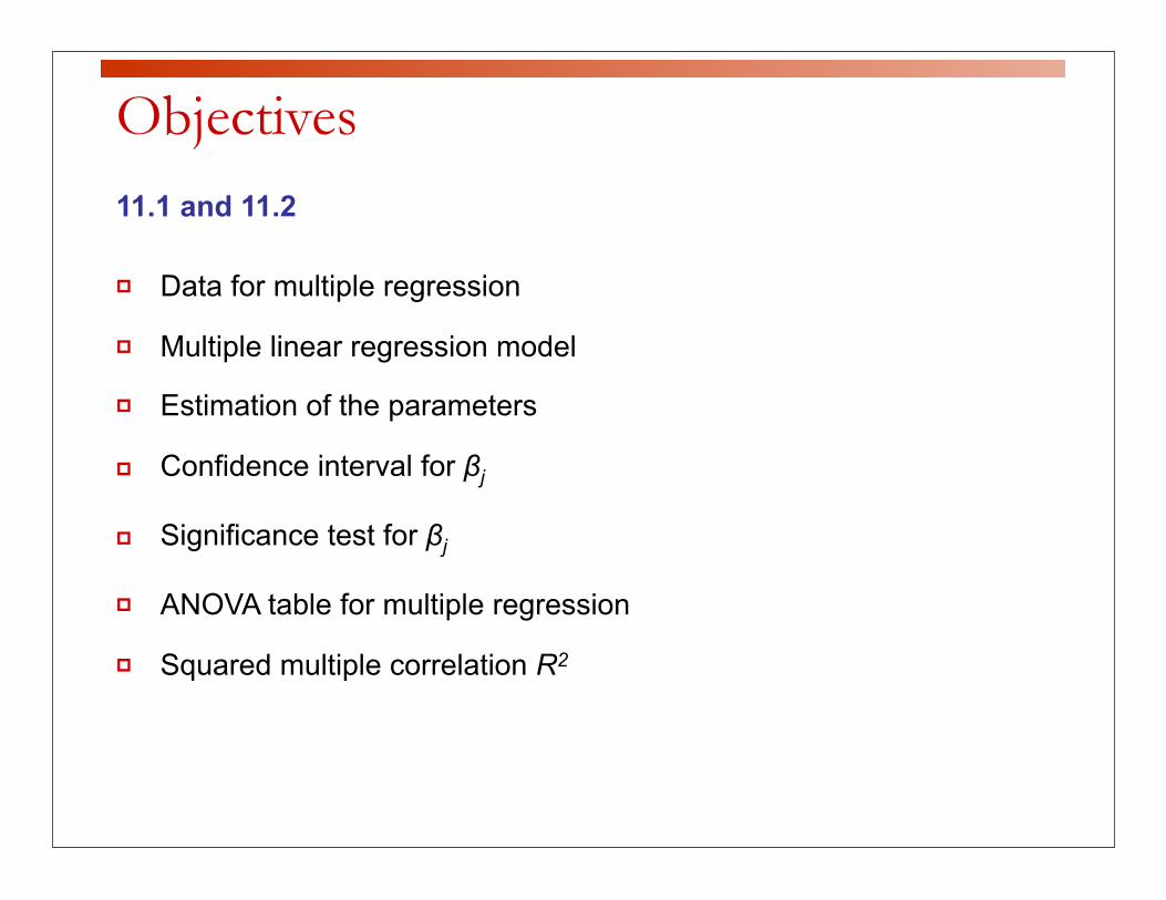
Objectives11.1 and 11.2

Data for multiple regression

Multiple linear regression model

Estimation of the parameters

Confidence interval for βj

Significance test for βj

ANOVA table for multiple regression

Squared multiple correlation R2

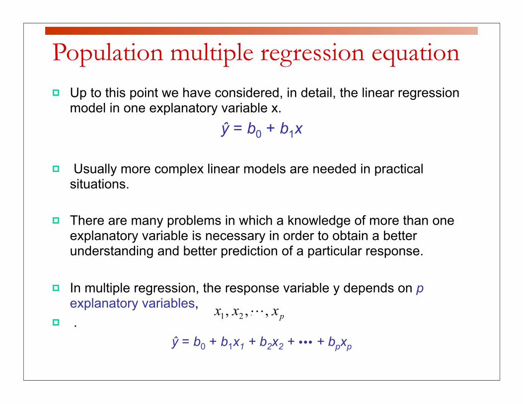
Population multiple regression equation Up to this point we have considered, in detail, the linear regression

model in one explanatory variable x.ŷ = b0 + b1x

Usually more complex linear models are needed in practical situations.

There are many problems in which a knowledge of more than one explanatory variable is necessary in order to obtain a better understanding and better prediction of a particular response.

In multiple regression, the response variable y depends on p explanatory variables,

.ŷ = b0 + b1x1 + b2x2 + + bpxp

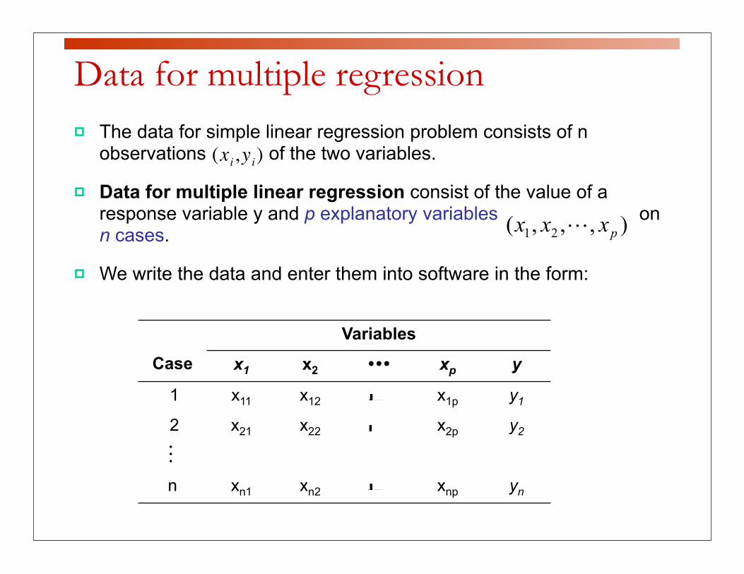
Data for multiple regression The data for simple linear regression problem consists of n

observations of the two variables.

Data for multiple linear regression consist of the value of a response variable y and p explanatory variables on n cases.

We write the data and enter them into software in the form:

Variables

Case x1 x2 xp y

1 x11 x12 x1p y1

2 x21 x22 x2p y2

n xn1 xn2 xnp yn

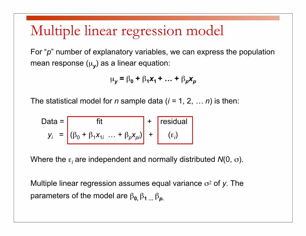
For “p” number of explanatory variables, we can express the population mean response (µy) as a linear equation:

µy = β0 + β1x1 + … + βpxp

The statistical model for n sample data (i = 1, 2, … n) is then:

Data = fit + residual

yi = (β0 + β1x1i … + βpxpi) + (εi)

Where the εi are independent and normally distributed N(0, σ).

Multiple linear regression assumes equal variance σ2 of y. The parameters of the model are β0, β1 … βp.

Multiple linear regression model

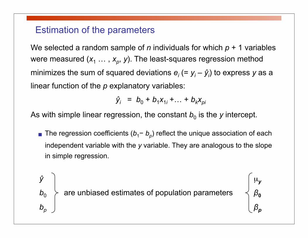
We selected a random sample of n individuals for which p + 1 variables were measured (x1 … , xp, y). The least-squares regression method

minimizes the sum of squared deviations ei (= yi – ŷi) to express y as a

linear function of the p explanatory variables:

ŷi = b0 + b1x1i +… + bkxpi

As with simple linear regression, the constant b0 is the y intercept.

■ The regression coefficients (b1− bp) reflect the unique association of each

independent variable with the y variable. They are analogous to the slope in simple regression.

ŷ µy

b0 are unbiased estimates of population parameters β0

bp βp

Estimation of the parameters

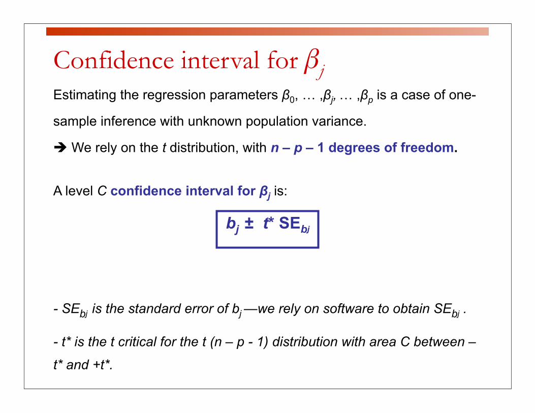
Confidence interval for βjEstimating the regression parameters β0, … ,βj, … ,βp is a case of one-

sample inference with unknown population variance.

We rely on the t distribution, with n – p – 1 degrees of freedom.

A level C confidence interval for βj is:

bj ± t* SEbj

- SEbj is the standard error of bj —we rely on software to obtain SEbj .

- t* is the t critical for the t (n – p - 1) distribution with area C between –

t* and +t*.

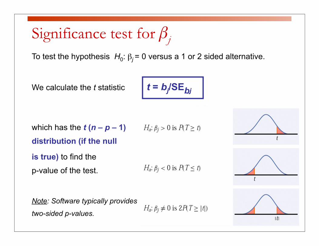
Significance test for βjTo test the hypothesis H0: βj = 0 versus a 1 or 2 sided alternative.

We calculate the t statistic t = bj/SEbj

which has the t (n – p – 1) distribution (if the null

is true) to find the

p-value of the test.

Note: Software typically provides

two-sided p-values.

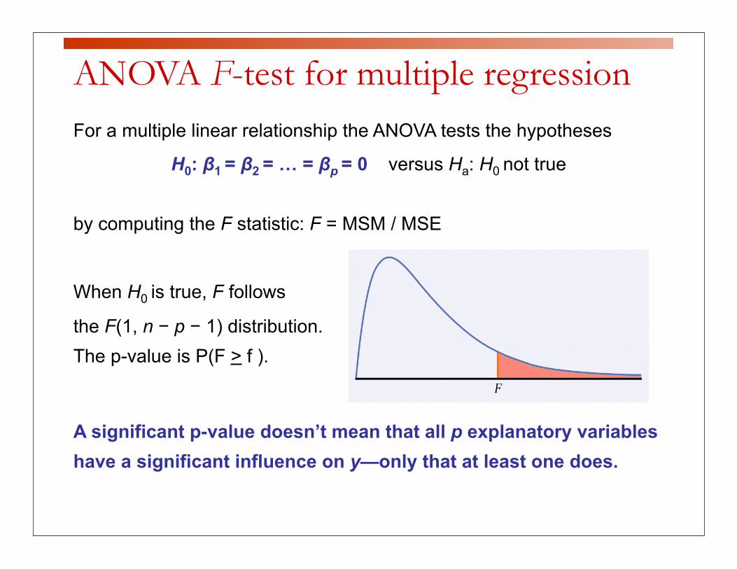
For a multiple linear relationship the ANOVA tests the hypotheses

H0: β1 = β2 = … = βp = 0 versus Ha: H0 not true

by computing the F statistic: F = MSM / MSE

When H0 is true, F follows

the F(1, n − p − 1) distribution. The p-value is P(F > f ).

A significant p-value doesn’t mean that all p explanatory variables have a significant influence on y—only that at least one does.

ANOVA F-test for multiple regression

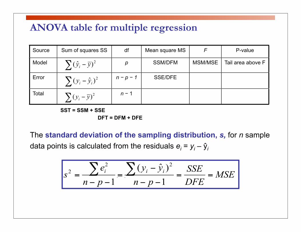
ANOVA table for multiple regression

Source Sum of squares SS df Mean square MS F P-value

Model p SSM/DFM MSM/MSE Tail area above F

Error n − p − 1 SSE/DFE

Total n − 1

SST = SSM + SSEDFT = DFM + DFE

The standard deviation of the sampling distribution, s, for n sample data points is calculated from the residuals ei = yi – ŷi

s is an unbiased estimate of the regression standard deviation σ.

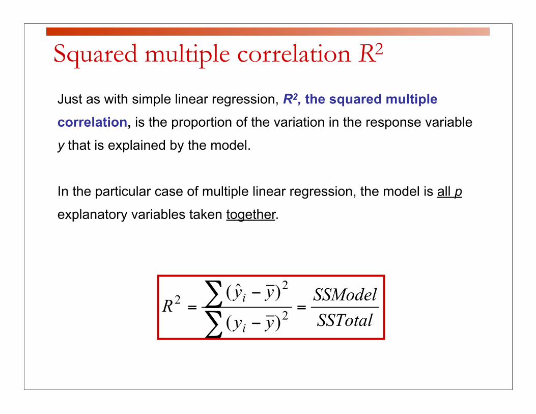
Squared multiple correlation R2

Just as with simple linear regression, R2, the squared multiple correlation, is the proportion of the variation in the response variable

y that is explained by the model.

In the particular case of multiple linear regression, the model is all p

explanatory variables taken together.

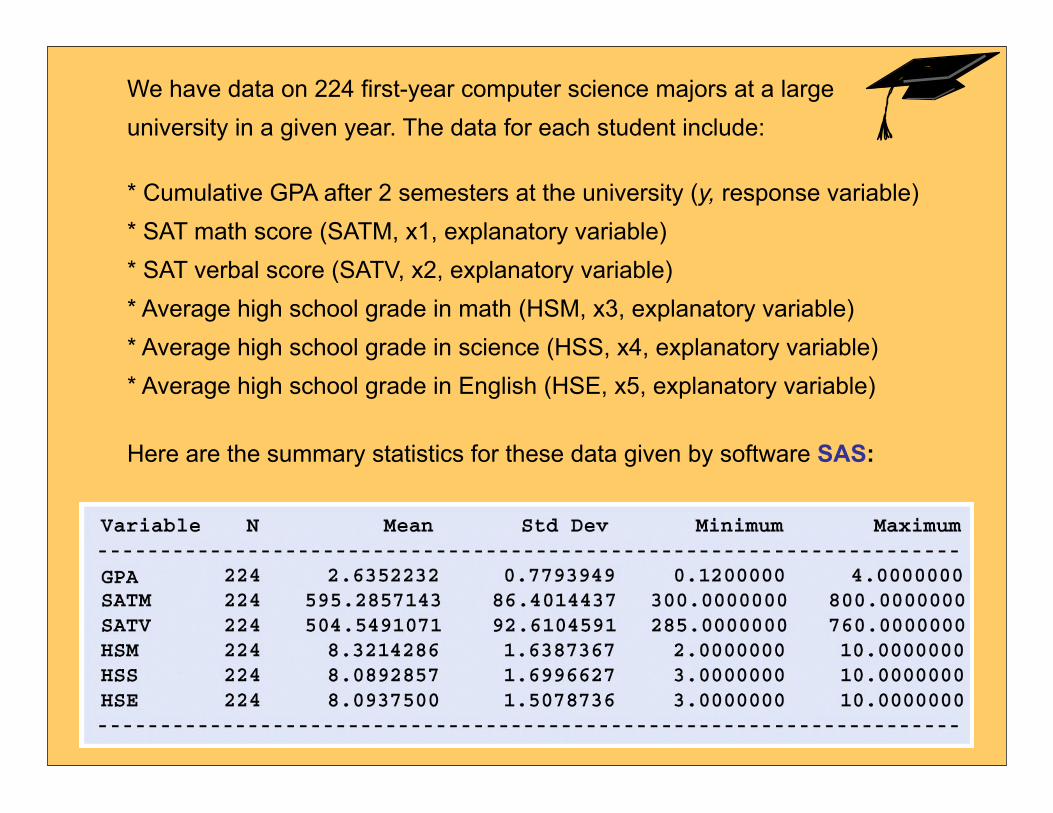
We have data on 224 first-year computer science majors at a large university in a given year. The data for each student include:

* Cumulative GPA after 2 semesters at the university (y, response variable)* SAT math score (SATM, x1, explanatory variable)* SAT verbal score (SATV, x2, explanatory variable)* Average high school grade in math (HSM, x3, explanatory variable)* Average high school grade in science (HSS, x4, explanatory variable)* Average high school grade in English (HSE, x5, explanatory variable)

Here are the summary statistics for these data given by software SAS:

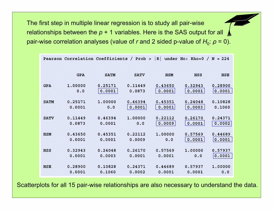
The first step in multiple linear regression is to study all pair-wise relationships between the p + 1 variables. Here is the SAS output for all pair-wise correlation analyses (value of r and 2 sided p-value of H0: ρ = 0).

Scatterplots for all 15 pair-wise relationships are also necessary to understand the data.

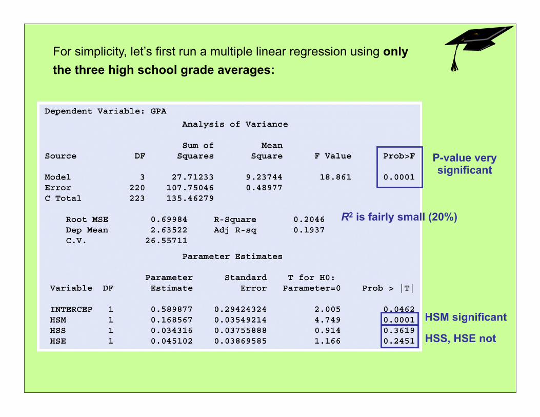
For simplicity, let’s first run a multiple linear regression using only the three high school grade averages:

P-value very significant

R2 is fairly small (20%)

HSM significant

HSS, HSE not

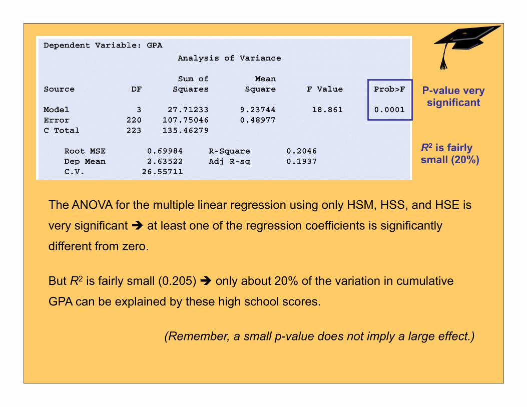
The ANOVA for the multiple linear regression using only HSM, HSS, and HSE is

very significant at least one of the regression coefficients is significantly

different from zero.

But R2 is fairly small (0.205) only about 20% of the variation in cumulative

GPA can be explained by these high school scores.

(Remember, a small p-value does not imply a large effect.)

P-value very significant

R2 is fairly small (20%)

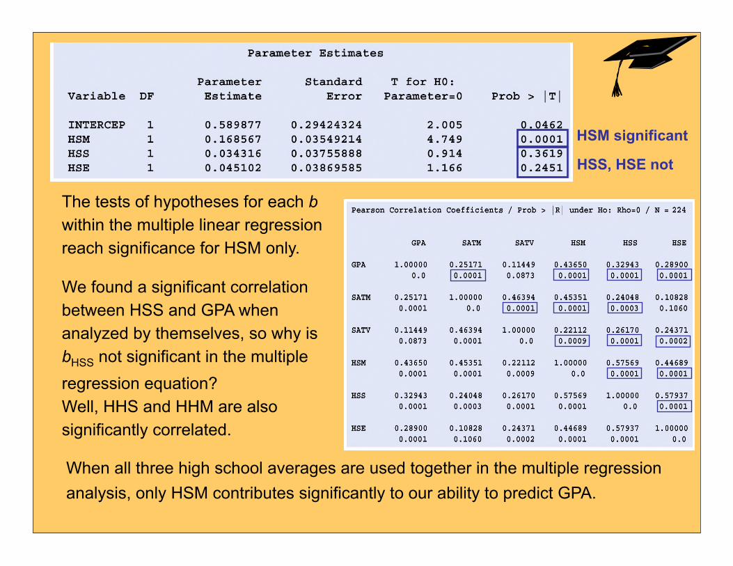
The tests of hypotheses for each b within the multiple linear regression reach significance for HSM only.

We found a significant correlation between HSS and GPA when analyzed by themselves, so why is bHSS not significant in the multiple regression equation?Well, HHS and HHM are also significantly correlated.

HSM significant

HSS, HSE not

When all three high school averages are used together in the multiple regression analysis, only HSM contributes significantly to our ability to predict GPA.

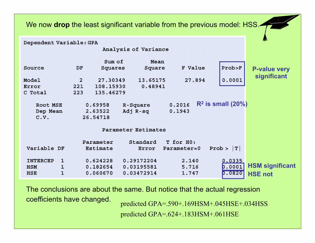
P-value very significant

R2 is small (20%)

HSM significantHSE not

We now drop the least significant variable from the previous model: HSS.

The conclusions are about the same. But notice that the actual regression coefficients have changed.

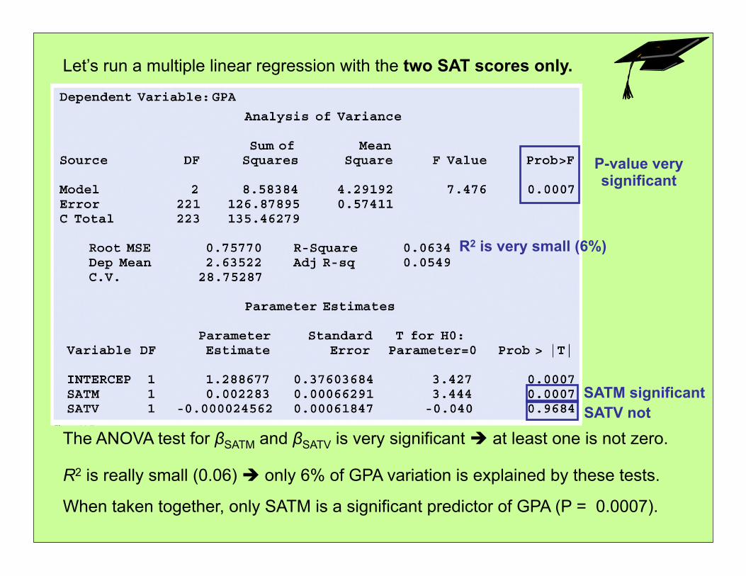
P-value very significant

R2 is very small (6%)

SATM significantSATV not

Let’s run a multiple linear regression with the two SAT scores only.

The ANOVA test for βSATM and βSATV is very significant at least one is not zero.

R2 is really small (0.06) only 6% of GPA variation is explained by these tests.

When taken together, only SATM is a significant predictor of GPA (P = 0.0007).

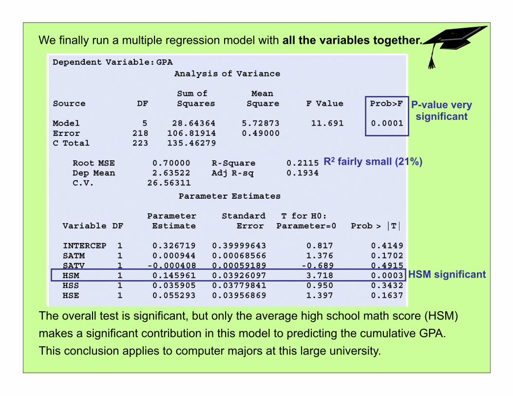
We finally run a multiple regression model with all the variables together.

The overall test is significant, but only the average high school math score (HSM) makes a significant contribution in this model to predicting the cumulative GPA.This conclusion applies to computer majors at this large university.

P-value very significant

R2 fairly small (21%)

HSM significant

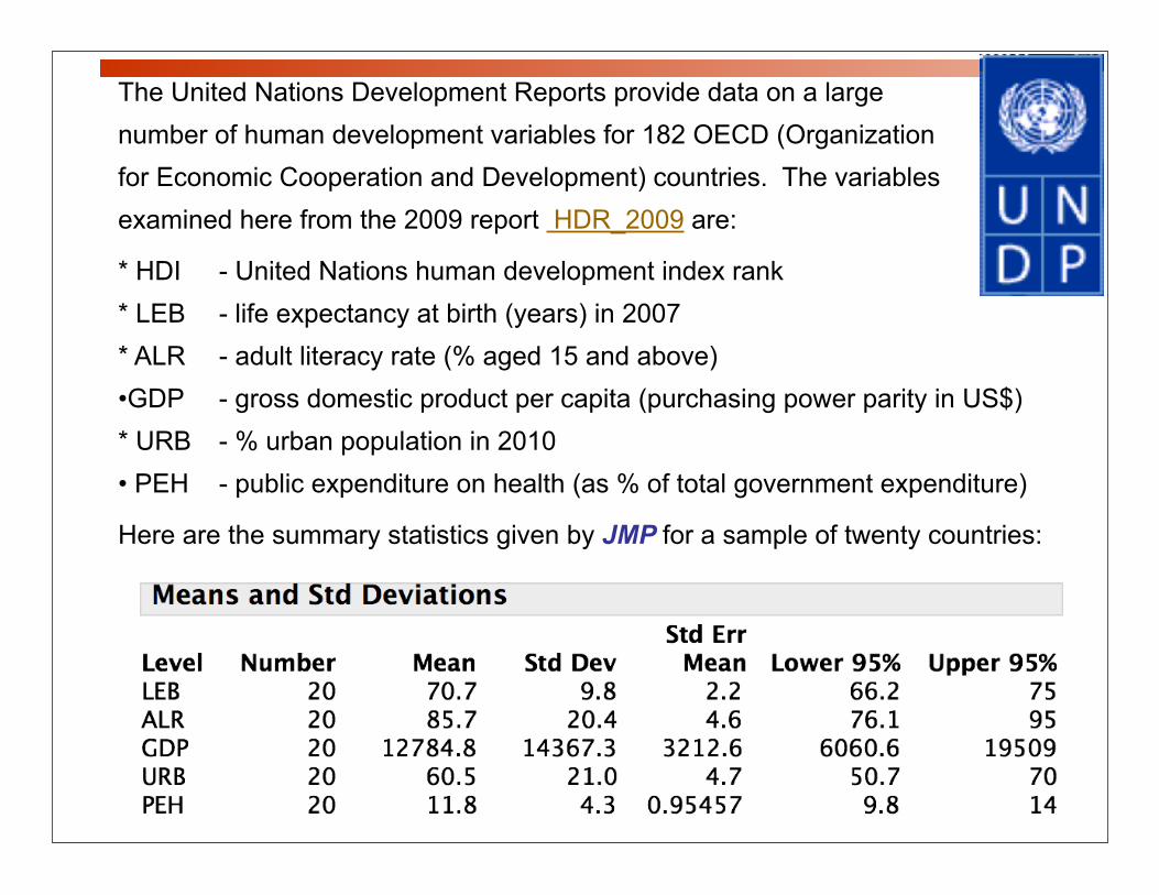
The United Nations Development Reports provide data on a large number of human development variables for 182 OECD (Organization for Economic Cooperation and Development) countries. The variables examined here from the 2009 report HDR_2009 are:

* HDI - United Nations human development index rank* LEB - life expectancy at birth (years) in 2007* ALR - adult literacy rate (% aged 15 and above)•GDP - gross domestic product per capita (purchasing power parity in US$)* URB - % urban population in 2010• PEH - public expenditure on health (as % of total government expenditure)

Here are the summary statistics given by JMP for a sample of twenty countries:

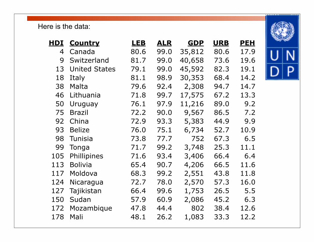
Here is the data:

HDI Country LEB ALR GDP URB PEH4 Canada 80.6 99.0 35,812 80.6 17.99 Switzerland 81.7 99.0 40,658 73.6 19.6

13 United States 79.1 99.0 45,592 82.3 19.118 Italy 81.1 98.9 30,353 68.4 14.238 Malta 79.6 92.4 2,308 94.7 14.746 Lithuania 71.8 99.7 17,575 67.2 13.350 Uruguay 76.1 97.9 11,216 89.0 9.275 Brazil 72.2 90.0 9,567 86.5 7.292 China 72.9 93.3 5,383 44.9 9.993 Belize 76.0 75.1 6,734 52.7 10.998 Tunisia 73.8 77.7 752 67.3 6.599 Tonga 71.7 99.2 3,748 25.3 11.1

105 Phillipines 71.6 93.4 3,406 66.4 6.4113 Bolivia 65.4 90.7 4,206 66.5 11.6117 Moldova 68.3 99.2 2,551 43.8 11.8124 Nicaragua 72.7 78.0 2,570 57.3 16.0127 Tajikistan 66.4 99.6 1,753 26.5 5.5150 Sudan 57.9 60.9 2,086 45.2 6.3172 Mozambique 47.8 44.4 802 38.4 12.6178 Mali 48.1 26.2 1,083 33.3 12.2

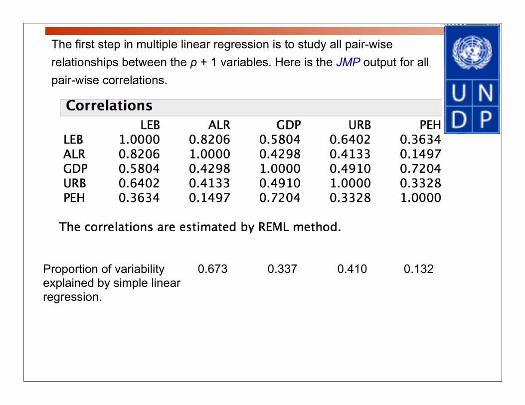
The first step in multiple linear regression is to study all pair-wise relationships between the p + 1 variables. Here is the JMP output for all pair-wise correlations.

Proportion of variability 0.673 0.337 0.410 0.132explained by simple linearregression.

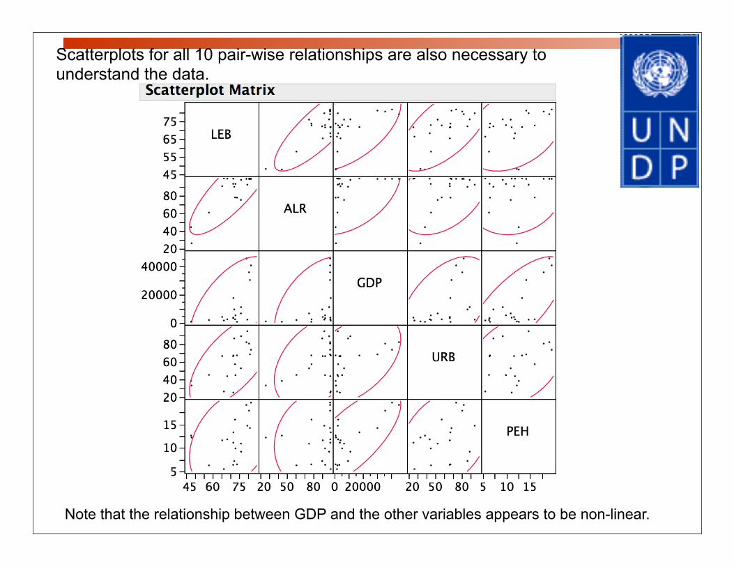
Scatterplots for all 10 pair-wise relationships are also necessary to understand the data.

Note that the relationship between GDP and the other variables appears to be non-linear.

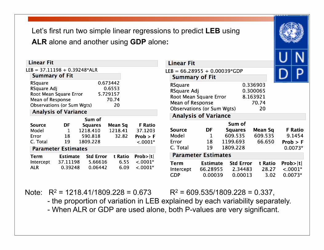
Let’s first run two simple linear regressions to predict LEB using ALR alone and another using GDP alone:

Note: R2 = 1218.41/1809.228 = 0.673 R2 = 609.535/1809.228 = 0.337, - the proportion of variation in LEB explained by each variability separately. - When ALR or GDP are used alone, both P-values are very significant.

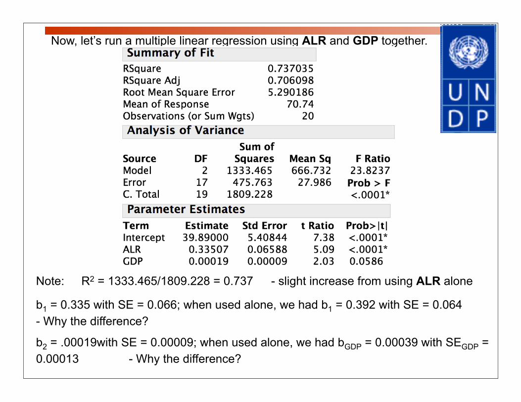
Now, let’s run a multiple linear regression using ALR and GDP together.

Note: R2 = 1333.465/1809.228 = 0.737 - slight increase from using ALR alone

b1 = 0.335 with SE = 0.066; when used alone, we had b1 = 0.392 with SE = 0.064- Why the difference?

b2 = .00019with SE = 0.00009; when used alone, we had bGDP = 0.00039 with SEGDP = 0.00013 - Why the difference?

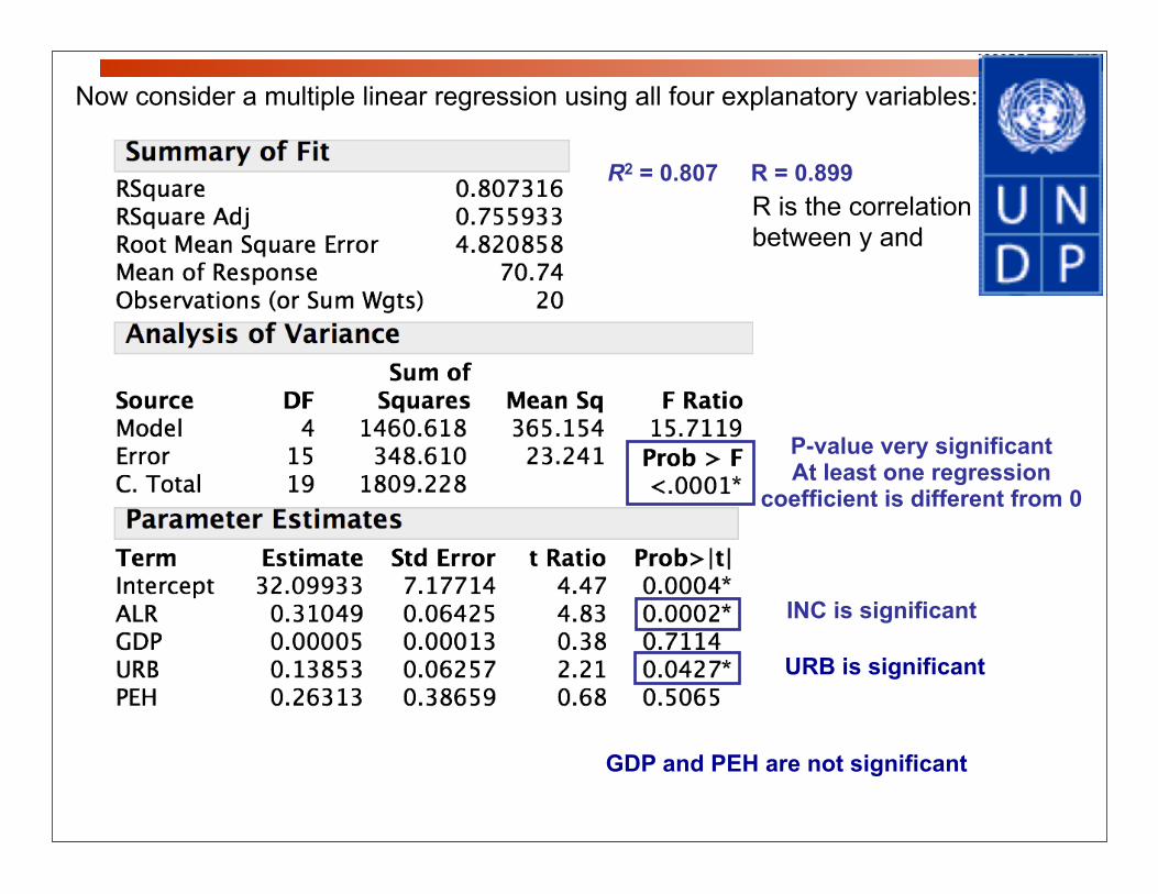
Now consider a multiple linear regression using all four explanatory variables:

P-value very significantAt least one regression

coefficient is different from 0

R2 = 0.807 R = 0.899

INC is significant

R is the correlation between y and

URB is significant

GDP and PEH are not significant

P-value very significant

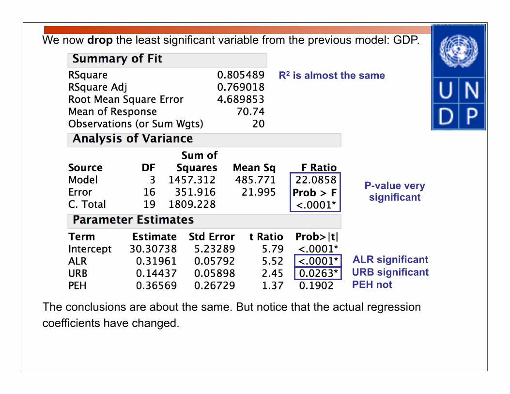
R2 is almost the same

ALR significant

PEH not

We now drop the least significant variable from the previous model: GDP.

The conclusions are about the same. But notice that the actual regression coefficients have changed.

URB significant

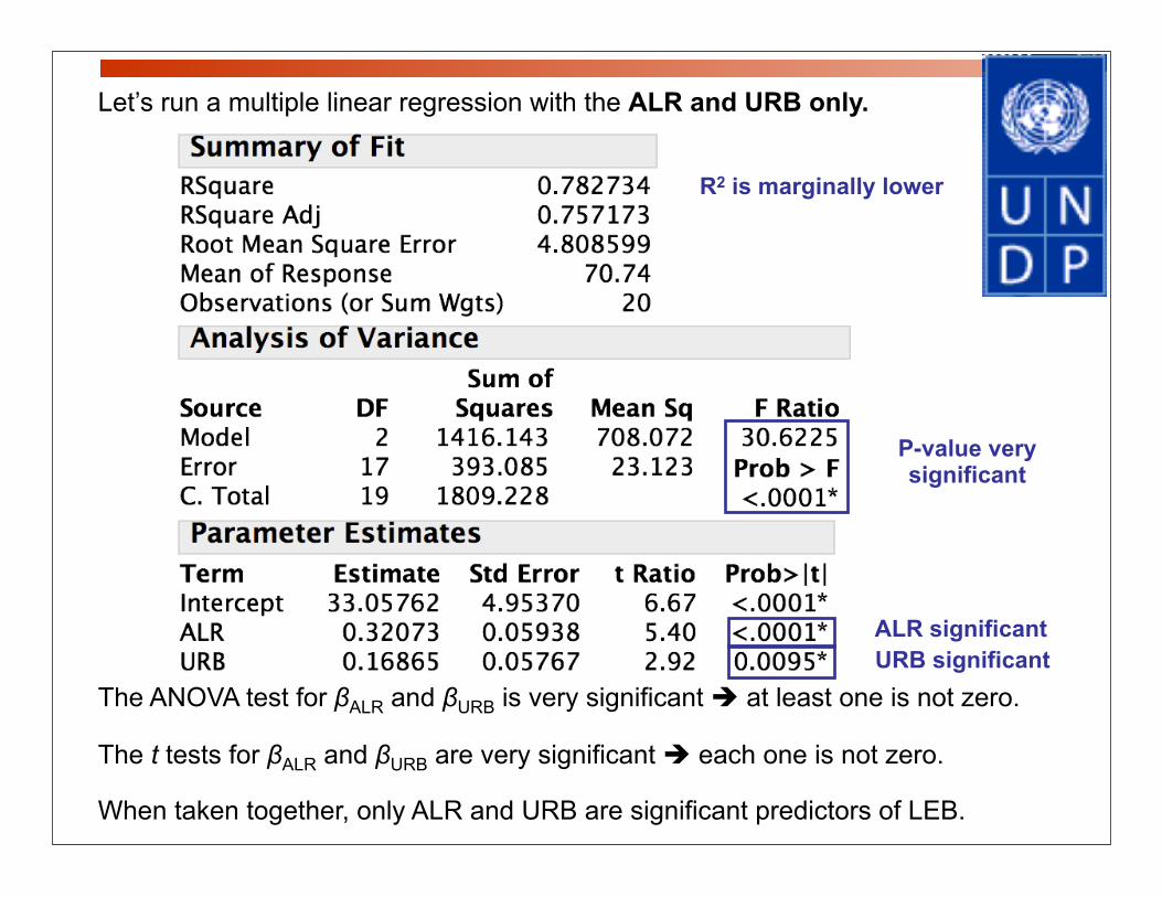
The ANOVA test for βALR and βURB is very significant at least one is not zero.

The t tests for βALR and βURB are very significant each one is not zero.

When taken together, only ALR and URB are significant predictors of LEB.

P-value very significant

R2 is marginally lower

ALR significantURB significant

Let’s run a multiple linear regression with the ALR and URB only.