Multiple Regression

S Vijay Ganesh

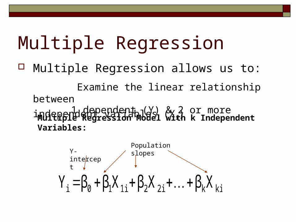
Multiple Regression Multiple Regression allows us to:

Examine the linear relationship between 1 dependent (Y) & 2 or more independent variables (Xi)

kik2i21i10i XβXβXββY

Multiple Regression Model with k Independent Variables:

Y-interceptPopulation slopes

Multiple Regression

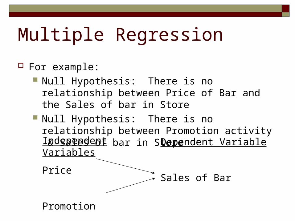
For example: Null Hypothesis: There is no relationship between Price of

Bar and the Sales of bar in Store Null Hypothesis: There is no relationship between

Promotion activity & Sales of bar in Store

Independent Variables

Price

Promotion

Dependent Variable

Sales of Bar

Multiple Regression

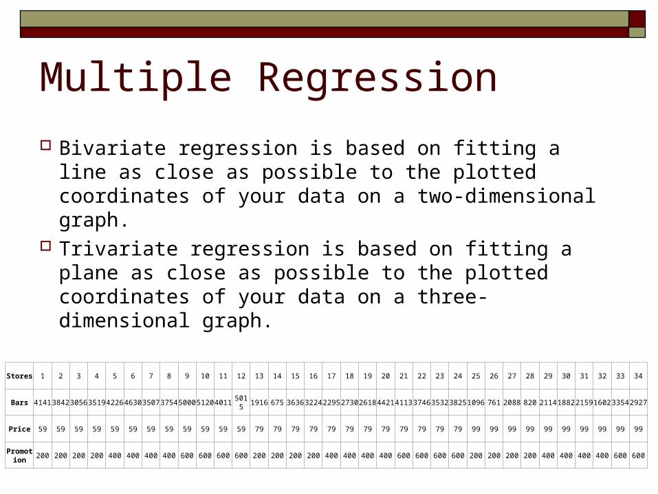
Bivariate regression is based on fitting a line as close as possible to the plotted coordinates of your data on a two-dimensional graph.

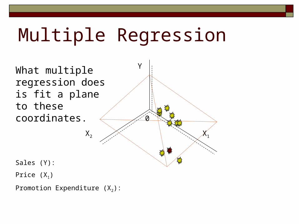
Trivariate regression is based on fitting a plane as close as possible to the plotted coordinates of your data on a three-dimensional graph.

Stores 1 2 3 4 5 6 7 8 9 10 11 12 13 14 15 16 17 18 19 20 21 22 23 24 25 26 27 28 29 30 31 32 33 34

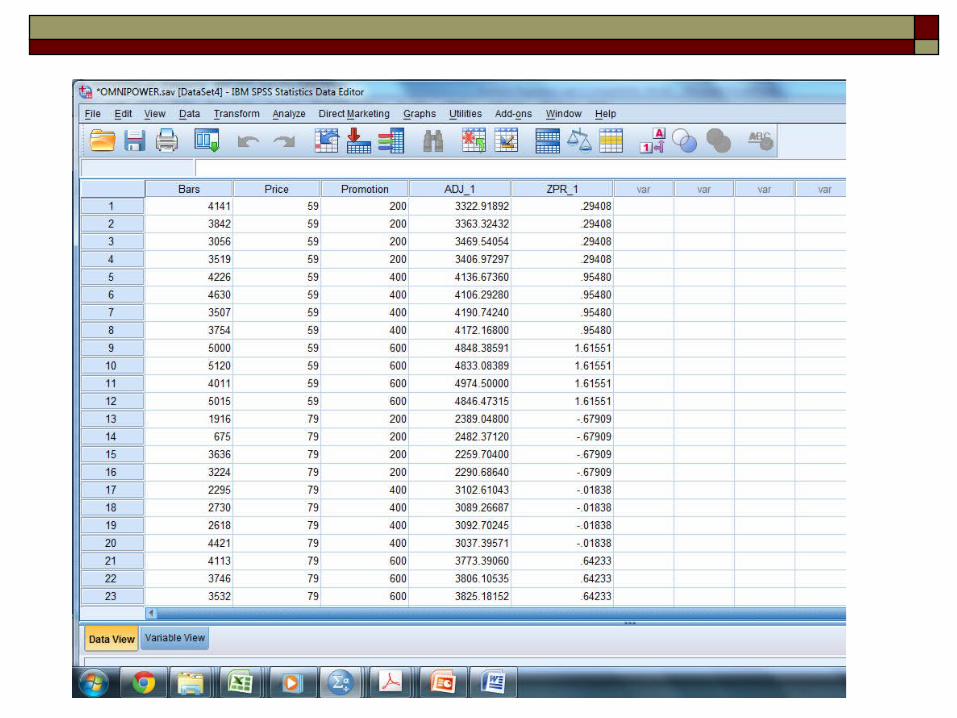
Bars 4141 3842 3056 3519 4226 4630 3507 3754 5000 5120 4011 5015 1916 675 3636 3224 2295 2730 2618 4421 4113 3746 3532 3825 1096 761 2088 820 2114 1882 2159 1602 3354 2927

Price 59 59 59 59 59 59 59 59 59 59 59 59 79 79 79 79 79 79 79 79 79 79 79 79 99 99 99 99 99 99 99 99 99 99

Promotion

200 200 200 200 400 400 400 400 600 600 600 600 200 200 200 200 400 400 400 400 600 600 600 600 200 200 200 200 400 400 400 400 600 600

Multiple Regression

Sales (Y):

Price (X1)

Promotion Expenditure (X2):

Y

X1X2

0

What multiple regression does is fit a plane to these coordinates.

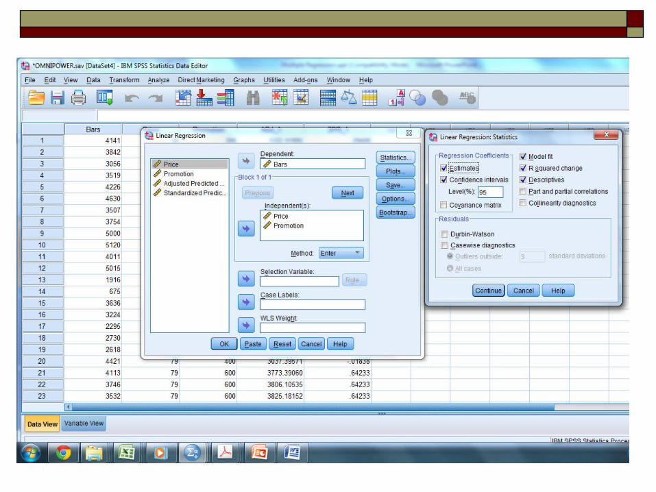
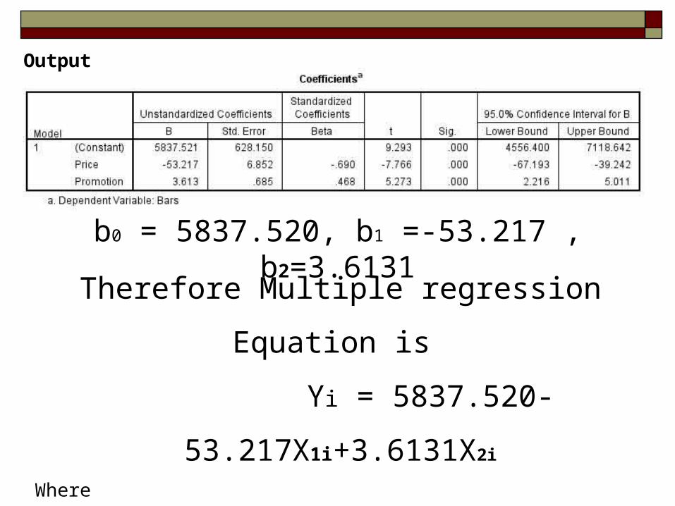
Output

b0 = 5837.520, b1 =-53.217 , b2=3.6131

Therefore Multiple regression Equation is

Yi = 5837.520-53.217X1i+3.6131X2i

Where

Yi= Predicated Monthly Sales of Bar for Store i

X1i= Price of Bar ( in Cent) for Store i

X2i=Monthly in Store Promotional Expenditure ( in Dollar) for Store i

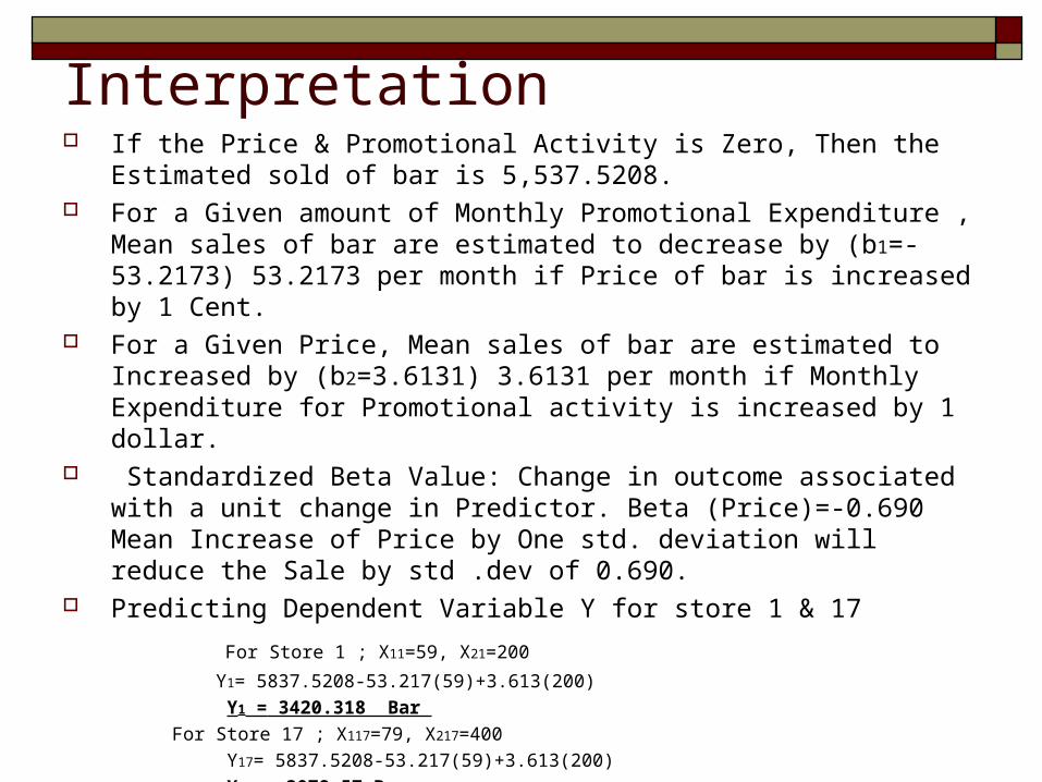
Interpretation If the Price & Promotional Activity is Zero, Then the Estimated sold of

bar is 5,537.5208. For a Given amount of Monthly Promotional Expenditure , Mean sales of

bar are estimated to decrease by (b1=-53.2173) 53.2173 per month if Price of bar is increased by 1 Cent.

For a Given Price, Mean sales of bar are estimated to Increased by (b2=3.6131) 3.6131 per month if Monthly Expenditure for Promotional activity is increased by 1 dollar.

Standardized Beta Value: Change in outcome associated with a unit change in Predictor. Beta (Price)=-0.690 Mean Increase of Price by One std. deviation will reduce the Sale by std .dev of 0.690.

Predicting Dependent Variable Y for store 1 & 17

For Store 1 ; X11=59, X21=200

Y1= 5837.5208-53.217(59)+3.613(200)

Y1 = 3420.318 Bar

For Store 17 ; X117=79, X217=400

Y17= 5837.5208-53.217(59)+3.613(200)

Y17 = 3078.57 Bar

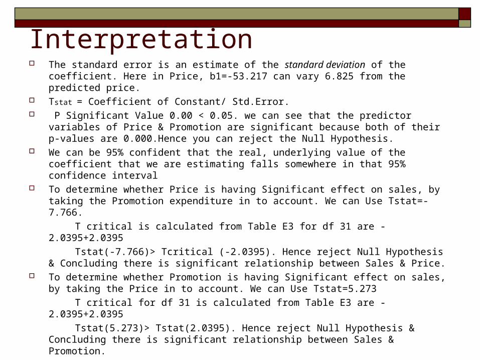
Interpretation The standard error is an estimate of the standard deviation of the coefficient. Here

in Price, b1=-53.217 can vary 6.825 from the predicted price. Tstat = Coefficient of Constant/ Std.Error. P Significant Value 0.00 < 0.05. we can see that the predictor variables of Price

& Promotion are significant because both of their p-values are 0.000.Hence you can reject the Null Hypothesis.

We can be 95% confident that the real, underlying value of the coefficient that we are estimating falls somewhere in that 95% confidence interval

To determine whether Price is having Significant effect on sales, by taking the Promotion expenditure in to account. We can Use Tstat=-7.766.

T critical is calculated from Table E3 for df 31 are -2.0395+2.0395

Tstat(-7.766)> Tcritical (-2.0395). Hence reject Null Hypothesis & Concluding there is significant relationship between Sales & Price.

To determine whether Promotion is having Significant effect on sales, by taking the Price in to account. We can Use Tstat=5.273

T critical for df 31 is calculated from Table E3 are -2.0395+2.0395

Tstat(5.273)> Tstat(2.0395). Hence reject Null Hypothesis & Concluding there is significant relationship between Sales & Promotion.

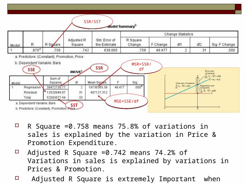
SSRSSRSSESSE

SSTSSTMSE=SSE/dfMSE=SSE/df

MSR=SSR/dfMSR=SSR/df

R Square =0.758 means 75.8% of variations in sales is explained by the variation in Price & Promotion Expenditure.

Adjusted R Square =0.742 means 74.2% of Variations in sales is explained by variations in Prices & Promotion.

Adjusted R Square is extremely Important when you are comparing two or more regression Model that predict same dependent variable but have a different Independent Variable.

SSR/SSTSSR/SST

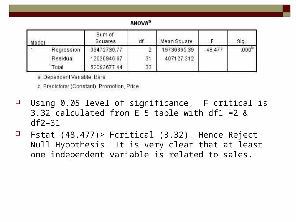
Using 0.05 level of significance, F critical is 3.32 calculated from E 5 table with df1 =2 & df2=31

Fstat (48.477)> Fcritical (3.32). Hence Reject Null Hypothesis. It is very clear that at least one independent variable is related to sales.

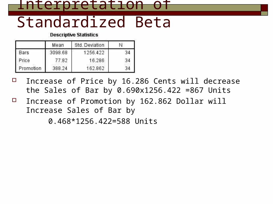
Increase of Price by 16.286 Cents will decrease the Sales of Bar by 0.690x1256.422 =867 Units

Increase of Promotion by 162.862 Dollar will Increase Sales of Bar by

0.468*1256.422=588 Units

Interpretation of Standardized Beta

Thank you