Chapter 6 Multiple Regression

Timothy Hanson

Department of Statistics, University of South Carolina

Stat 704: Data Analysis I

1 / 25

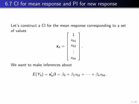
6.7 CI for mean response and PI for new response

Let’s construct a CI for the mean response corresponding to a setof values

xh =

1xh1xh2

...xhk

.We want to make inferences about

E (Yh) = x′hβ = β0 + β1xh1 + · · ·+ βkxhk .

2 / 25

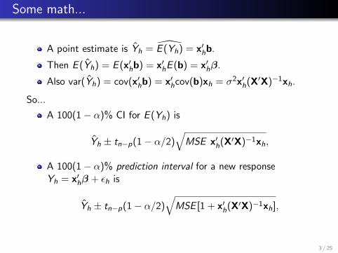
Some math...

A point estimate is Yh = E (Yh) = x′hb.

Then E (Yh) = E (x′hb) = x′hE (b) = x′hβ.

Also var(Yh) = cov(x′hb) = x′hcov(b)xh = σ2x′h(X′X)−1xh.

So...

A 100(1− α)% CI for E (Yh) is

Yh ± tn−p(1− α/2)√MSE x′h(X′X)−1xh,

A 100(1− α)% prediction interval for a new responseYh = x′hβ + εh is

Yh ± tn−p(1− α/2)√MSE [1 + x′h(X′X)−1xh],

3 / 25

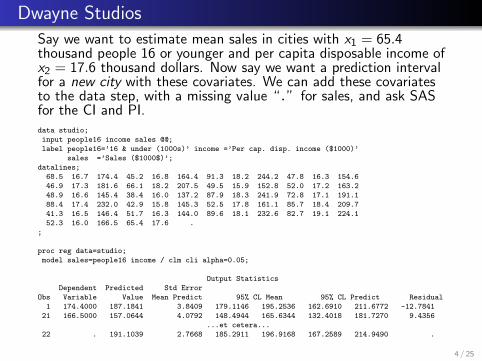
Dwayne Studios

Say we want to estimate mean sales in cities with x1 = 65.4thousand people 16 or younger and per capita disposable income ofx2 = 17.6 thousand dollars. Now say we want a prediction intervalfor a new city with these covariates. We can add these covariatesto the data step, with a missing value “.” for sales, and ask SASfor the CI and PI.data studio;

input people16 income sales @@;

label people16=’16 & under (1000s)’ income =’Per cap. disp. income ($1000)’

sales =’Sales ($1000$)’;

datalines;

68.5 16.7 174.4 45.2 16.8 164.4 91.3 18.2 244.2 47.8 16.3 154.6

46.9 17.3 181.6 66.1 18.2 207.5 49.5 15.9 152.8 52.0 17.2 163.2

48.9 16.6 145.4 38.4 16.0 137.2 87.9 18.3 241.9 72.8 17.1 191.1

88.4 17.4 232.0 42.9 15.8 145.3 52.5 17.8 161.1 85.7 18.4 209.7

41.3 16.5 146.4 51.7 16.3 144.0 89.6 18.1 232.6 82.7 19.1 224.1

52.3 16.0 166.5 65.4 17.6 .

;

proc reg data=studio;

model sales=people16 income / clm cli alpha=0.05;

Output Statistics

Dependent Predicted Std Error

Obs Variable Value Mean Predict 95% CL Mean 95% CL Predict Residual

1 174.4000 187.1841 3.8409 179.1146 195.2536 162.6910 211.6772 -12.7841

21 166.5000 157.0644 4.0792 148.4944 165.6344 132.4018 181.7270 9.4356

...et cetera...

22 . 191.1039 2.7668 185.2911 196.9168 167.2589 214.9490 .

4 / 25

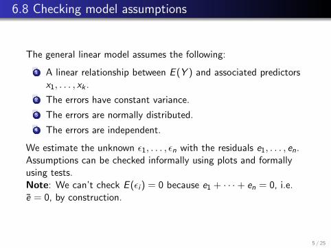
6.8 Checking model assumptions

The general linear model assumes the following:

1 A linear relationship between E (Y ) and associated predictorsx1, . . . , xk .

2 The errors have constant variance.

3 The errors are normally distributed.

4 The errors are independent.

We estimate the unknown ε1, . . . , εn with the residuals e1, . . . , en.Assumptions can be checked informally using plots and formallyusing tests.Note: We can’t check E (εi ) = 0 because e1 + · · ·+ en = 0, i.e.e = 0, by construction.

5 / 25

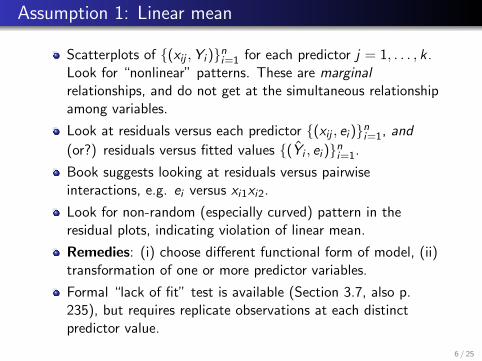
Assumption 1: Linear mean

Scatterplots of {(xij ,Yi )}ni=1 for each predictor j = 1, . . . , k .Look for “nonlinear” patterns. These are marginalrelationships, and do not get at the simultaneous relationshipamong variables.

Look at residuals versus each predictor {(xij , ei )}ni=1, and

(or?) residuals versus fitted values {(Yi , ei )}ni=1.

Book suggests looking at residuals versus pairwiseinteractions, e.g. ei versus xi1xi2.

Look for non-random (especially curved) pattern in theresidual plots, indicating violation of linear mean.

Remedies: (i) choose different functional form of model, (ii)transformation of one or more predictor variables.

Formal “lack of fit” test is available (Section 3.7, also p.235), but requires replicate observations at each distinctpredictor value.

6 / 25

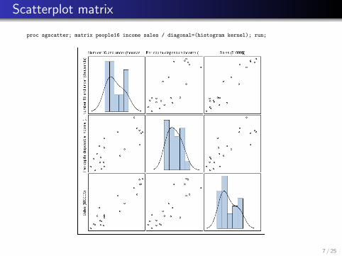
Scatterplot matrix

proc sgscatter; matrix people16 income sales / diagonal=(histogram kernel); run;

7 / 25

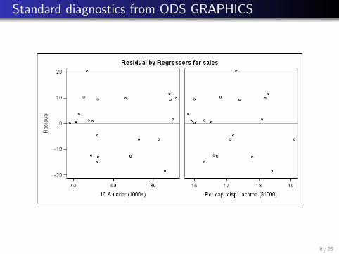
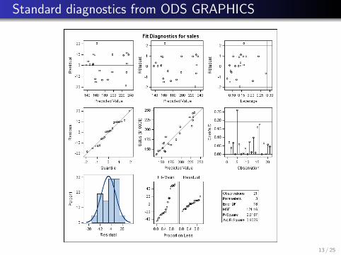
Standard diagnostics from ODS GRAPHICS

8 / 25

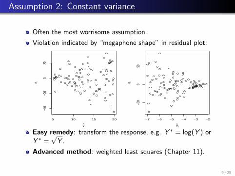
Assumption 2: Constant variance

Often the most worrisome assumption.

Violation indicated by “megaphone shape” in residual plot:

5 10 15 20

−40

−20

020

Yi

e i

−7 −6 −5 −4 −3 −2

−50

050

Yie i

Easy remedy: transform the response, e.g. Y ∗ = log(Y ) orY ∗ =

√Y .

Advanced method: weighted least squares (Chapter 11).

9 / 25

Non-constant variance

Breusch-Pagan test (pp. 118–119): tests whether the logerror variance increases or decreases linearly with thepredictor(s). Where Yi ∼ N(x′iβ, σ

2i ), set

log σ2i = α0 + α1xi1 + · · ·αkxik and testH0 : α1 = · · · = αk = 0, i.e. log σ2i = α0. Requires largesamples & assumes normal errors.

Brown-Forsythe test (pp. 116–117): Robust to non-normalerrors. Requires user to break data into groups and test forconstancy error variance across groups (not natural forcontinuous data).

Graphical methods have advantage of checking for generalviolations, not just violation of a specific type.

10 / 25

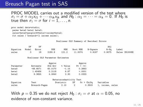
Breusch Pagan test in SAS

PROC MODEL carries out a modified version of the test whereσi = σ + α1xi1 + · · ·αikxik and H0 : α1 = · · · = αk = 0. If H0 istrue then σi = σ for i = 1, . . . , n.

proc model data=studio;

parms beta0 beta1 beta2;

sales=beta0+people16*beta1+income*beta2;

fit sales / breusch=(1 income sales);

Nonlinear OLS Summary of Residual Errors

DF DF Adj

Equation Model Error SSE MSE Root MSE R-Square R-Sq Label

sales 3 18 2180.9 121.2 11.0074 0.9167 0.9075 Sales ($1000$)

Nonlinear OLS Parameter Estimates

Approx Approx

Parameter Estimate Std Err t Value Pr > |t|

beta0 -68.8571 60.0170 -1.15 0.2663

beta1 1.45456 0.2118 6.87 <.0001

beta2 9.3655 4.0640 2.30 0.0333

Heteroscedasticity Test

Equation Test Statistic DF Pr > ChiSq Variables

sales Breusch-Pagan 2.10 2 0.3503 1, income, sales

With p = 0.35 we do not reject H0 : σi = σ at α = 0.05, noevidence of non-constant variance.

11 / 25

Assumption 3: errors are normally distributed

Caution: your estimate of ε, given by e = Y−Xb, is only as goodas the model for your mean! Changing the mean can drasticallychange the residuals e and any residual plots or formal tests basedon them. Diagnostics include...

Q-Q plot of e1, . . . , en.

Formal test for normality: Shapiro-Wilk (Section 3.5),essentially based on the correlation coefficient r for expectedversus observed in normal Q-Q plot.

Remedy: transformation of Y and or any of x1, . . . , xk ,nonparametric methods (e.g. additive models), robustregression (least sum of absolute distances), medianregression.

12 / 25

Standard diagnostics from ODS GRAPHICS

13 / 25

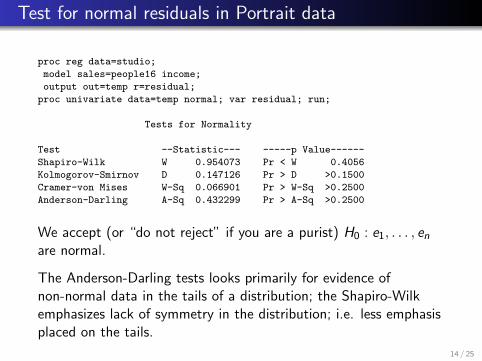
Test for normal residuals in Portrait data

proc reg data=studio;

model sales=people16 income;

output out=temp r=residual;

proc univariate data=temp normal; var residual; run;

Tests for Normality

Test --Statistic--- -----p Value------

Shapiro-Wilk W 0.954073 Pr < W 0.4056

Kolmogorov-Smirnov D 0.147126 Pr > D >0.1500

Cramer-von Mises W-Sq 0.066901 Pr > W-Sq >0.2500

Anderson-Darling A-Sq 0.432299 Pr > A-Sq >0.2500

We accept (or “do not reject” if you are a purist) H0 : e1, . . . , enare normal.

The Anderson-Darling tests looks primarily for evidence ofnon-normal data in the tails of a distribution; the Shapiro-Wilkemphasizes lack of symmetry in the distribution; i.e. less emphasisplaced on the tails.

14 / 25

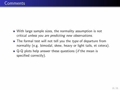
Comments

With large sample sizes, the normality assumption is notcritical unless you are predicting new observations.

The formal test will not tell you the type of departure fromnormality (e.g. bimodal, skew, heavy or light tails, et cetera).

Q-Q plots help answer these questions (if the mean isspecified correctly).

15 / 25

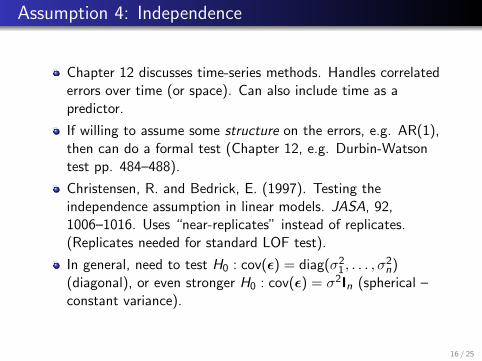
Assumption 4: Independence

Chapter 12 discusses time-series methods. Handles correlatederrors over time (or space). Can also include time as apredictor.

If willing to assume some structure on the errors, e.g. AR(1),then can do a formal test (Chapter 12, e.g. Durbin-Watsontest pp. 484–488).

Christensen, R. and Bedrick, E. (1997). Testing theindependence assumption in linear models. JASA, 92,1006–1016. Uses “near-replicates” instead of replicates.(Replicates needed for standard LOF test).

In general, need to test H0 : cov(ε) = diag(σ21, . . . , σ2n)

(diagonal), or even stronger H0 : cov(ε) = σ2In (spherical –constant variance).

16 / 25

Another example

Problems 6.15, 6.16, 6.17

Y = patient satisfaction (100 point scale)

x1 = age in years

x2 = illness severity (an index)

x3 = anxiety level (an index)

Let’s analyze these data with SAS...

17 / 25

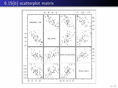
6.15(b) scatterplot matrix

18 / 25

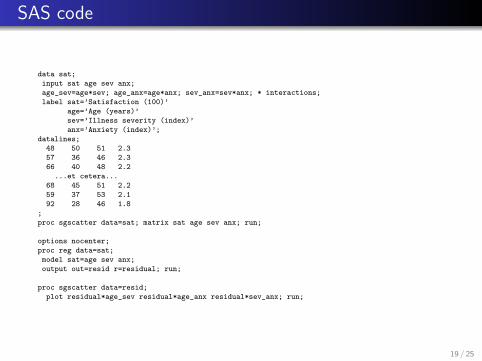
SAS code

data sat;

input sat age sev anx;

age_sev=age*sev; age_anx=age*anx; sev_anx=sev*anx; * interactions;

label sat=’Satisfaction (100)’

age=’Age (years)’

sev=’Illness severity (index)’

anx=’Anxiety (index)’;

datalines;

48 50 51 2.3

57 36 46 2.3

66 40 48 2.2

...et cetera...

68 45 51 2.2

59 37 53 2.1

92 28 46 1.8

;

proc sgscatter data=sat; matrix sat age sev anx; run;

options nocenter;

proc reg data=sat;

model sat=age sev anx;

output out=resid r=residual; run;

proc sgscatter data=resid;

plot residual*age_sev residual*age_anx residual*sev_anx; run;

19 / 25

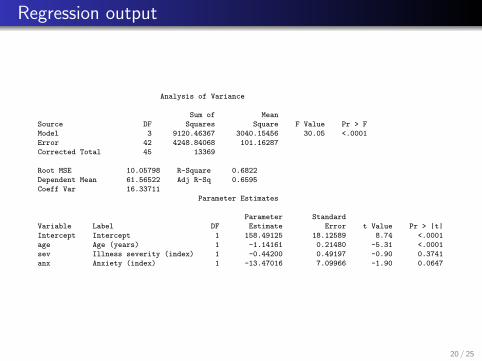
Regression output

Analysis of Variance

Sum of Mean

Source DF Squares Square F Value Pr > F

Model 3 9120.46367 3040.15456 30.05 <.0001

Error 42 4248.84068 101.16287

Corrected Total 45 13369

Root MSE 10.05798 R-Square 0.6822

Dependent Mean 61.56522 Adj R-Sq 0.6595

Coeff Var 16.33711

Parameter Estimates

Parameter Standard

Variable Label DF Estimate Error t Value Pr > |t|

Intercept Intercept 1 158.49125 18.12589 8.74 <.0001

age Age (years) 1 -1.14161 0.21480 -5.31 <.0001

sev Illness severity (index) 1 -0.44200 0.49197 -0.90 0.3741

anx Anxiety (index) 1 -13.47016 7.09966 -1.90 0.0647

20 / 25

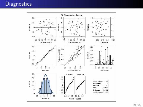
Diagnostics

21 / 25

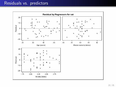
Residuals vs. predictors

22 / 25

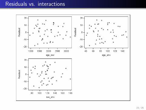
Residuals vs. interactions

23 / 25

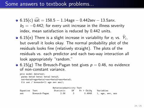
Some answers to textbook problems...

6.15(c) sat = 158.5− 1.14age− 0.442sev− 13.5anx.b2 = −0.442; for every unit increase in the illness severityindex, mean satisfaction is reduced by 0.442 units.

6.15(e) There is a slight increase in variability for ei vs. Yi ,but overall it looks okay. The normal probability plot of theresiduals looks fine (relatively straight). The plots of theresiduals vs. each predictor and each two-way interaction alllook appropriately “random.”

6.15(g) The Breusch-Pagan test gives p = 0.46, no evidenceof non-constant variance.proc model data=sat;

parms beta0 beta1 beta2 beta3;

sat=beta0+age*beta1+sev*beta2+anx*beta3;

fit sat / breusch=(1 age sev anx);

Heteroscedasticity Test

Equation Test Statistic DF Pr > ChiSq Variables

sat Breusch-Pagan 2.56 3 0.4648 1, age, sev, anx

24 / 25

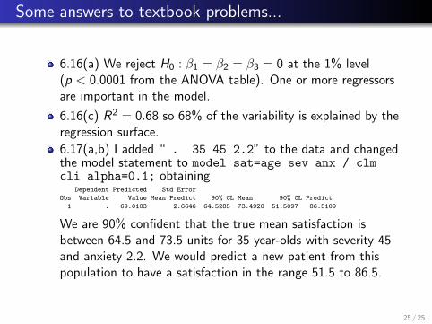
Some answers to textbook problems...

6.16(a) We reject H0 : β1 = β2 = β3 = 0 at the 1% level(p < 0.0001 from the ANOVA table). One or more regressorsare important in the model.

6.16(c) R2 = 0.68 so 68% of the variability is explained by theregression surface.

6.17(a,b) I added “ . 35 45 2.2” to the data and changedthe model statement to model sat=age sev anx / clmcli alpha=0.1; obtaining

Dependent Predicted Std Error

Obs Variable Value Mean Predict 90% CL Mean 90% CL Predict

1 . 69.0103 2.6646 64.5285 73.4920 51.5097 86.5109

We are 90% confident that the true mean satisfaction isbetween 64.5 and 73.5 units for 35 year-olds with severity 45and anxiety 2.2. We would predict a new patient from thispopulation to have a satisfaction in the range 51.5 to 86.5.

25 / 25