1

Research MethodResearch Method

Lecture 2 (Ch3)Lecture 2 (Ch3)

Multiple linear Multiple linear regressionregression

©

2

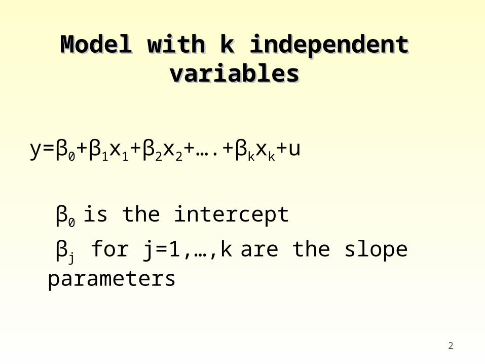
Model with k independent Model with k independent variablesvariables

y=β0+β1x1+β2x2+….+βkxk+u

β0 is the intercept

βj for j=1,…,k are the slope parameters

3

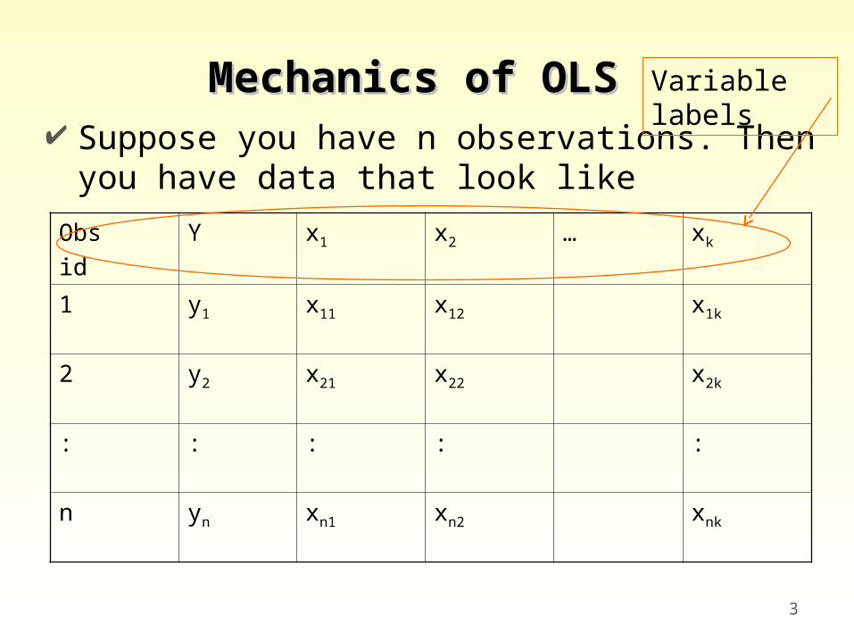
Mechanics of OLSMechanics of OLS Suppose you have n observations. Then you

have data that look like

Obs id

Y x1 x2 … xk

1 y1 x11 x12 x1k

2 y2 x21 x22 x2k

: : : : :

n yn xn1 xn2 xnk

Variable labels

4

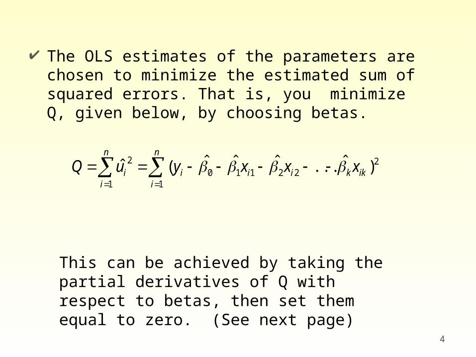
The OLS estimates of the parameters are chosen to minimize the estimated sum of squared errors. That is, you minimize Q, given below, by choosing betas.

222

1110

1

2 )ˆ...ˆˆˆ(ˆ ikki

n

iii

n

ii xxxyuQ

This can be achieved by taking the partial derivatives of Q with respect to betas, then set them equal to zero. (See next page)

5

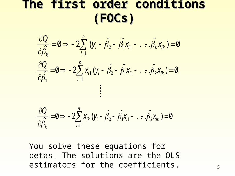
The first order conditions The first order conditions (FOCs)(FOCs)

0)ˆ...ˆˆ(20ˆ 11

101

1

ikki

n

iii xxyx

Q

0)ˆ...ˆˆ(20ˆ 11

10

0

ikki

n

ii xxy

Q

0)ˆ...ˆˆ(20ˆ 11

10

ikki

n

iiik

k

xxyxQ

……

.

You solve these equations for betas. The solutions are the OLS estimators for the coefficients.

6

Most common method to solve for the FOCs is to use matrix notation. We will use this method later.

For our purpose, more useful representation of the estimators are given in the next slide.

7

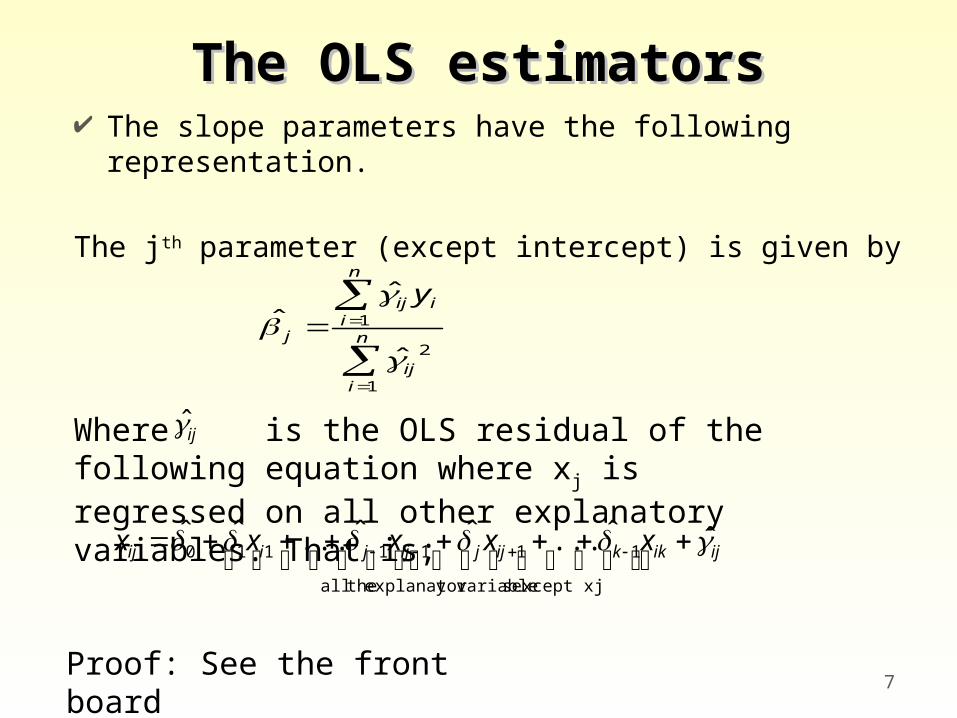
The OLS estimatorsThe OLS estimators The slope parameters have the following

representation.

The jth parameter (except intercept) is given by

n

iij

n

iiij

j

y

1

2

1

ˆ

ˆˆ

ijikkijjijjiij xxxxx ˆˆ...ˆˆ...ˆˆ

except xj sy variableexplanator theall

1111110

Where is the OLS residual of the following equation where xj is regressed on all other explanatory variables. That is;

Proof: See the front board

ij

8

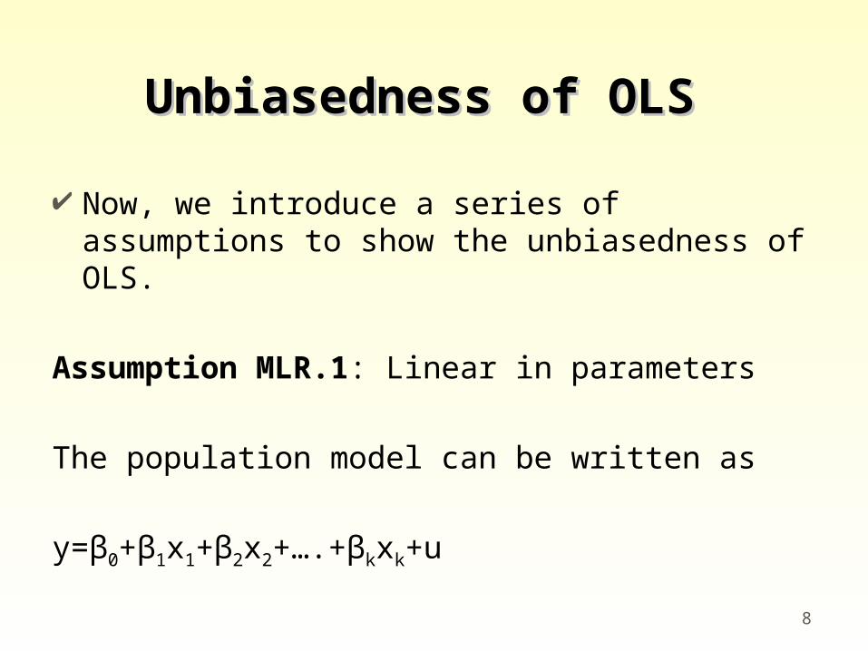
Unbiasedness of OLSUnbiasedness of OLS

Now, we introduce a series of assumptions to show the unbiasedness of OLS.

Assumption MLR.1: Linear in parameters

The population model can be written as

y=β0+β1x1+β2x2+….+βkxk+u

9

Assumption MLR.2: Random sampling

We have a random sample of n observations {xi1 xi2…xik, yi}, i=1,…,n following the population model.

10

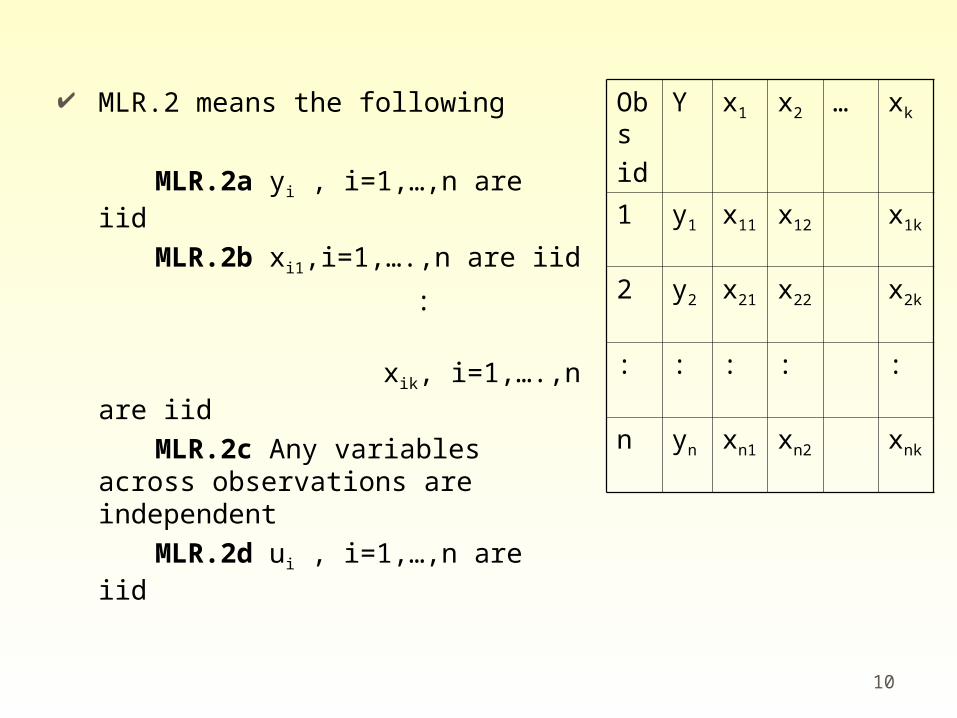
MLR.2 means the following

MLR.2a yi , i=1,…,n are iid

MLR.2b xi1,i=1,….,n are iid

: xik, i=1,….,n are iid

MLR.2c Any variables across observations are independent

MLR.2d ui , i=1,…,n are iid

Obs id

Y x1 x2 … xk

1 y1 x11 x12 x1k

2 y2 x21 x22 x2k

: : : : :

n yn xn1 xn2 xnk

11

Assumption MLR.3: No perfect collinearity

In the sample and in the population, none of the independent variables are constant, and there are no exact linear relationships among the independent variables.

12

Assumption MLR.4: Zero conditional mean

E(u|x1,x2,…,xk)=0

13

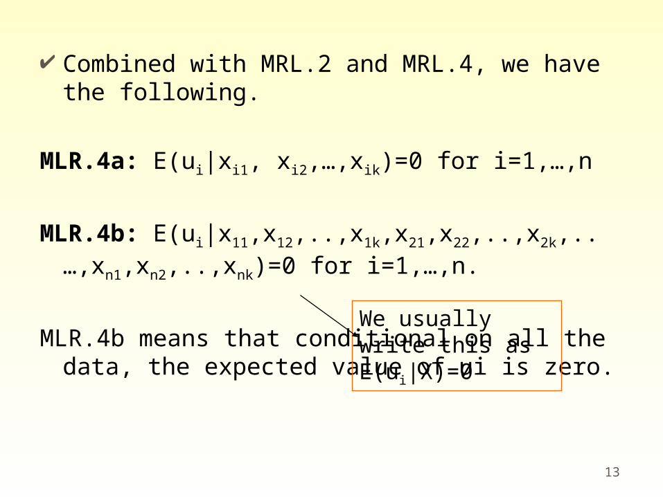
Combined with MRL.2 and MRL.4, we have the following.

MLR.4a: E(ui|xi1, xi2,…,xik)=0 for i=1,…,n

MLR.4b: E(ui|x11,x12,..,x1k,x21,x22,..,x2k,..…,xn1,xn2,..,xnk)=0 for i=1,…,n.

MLR.4b means that conditional on all the data, the expected value of ui is zero.

We usually write this as E(ui|X)=0

14

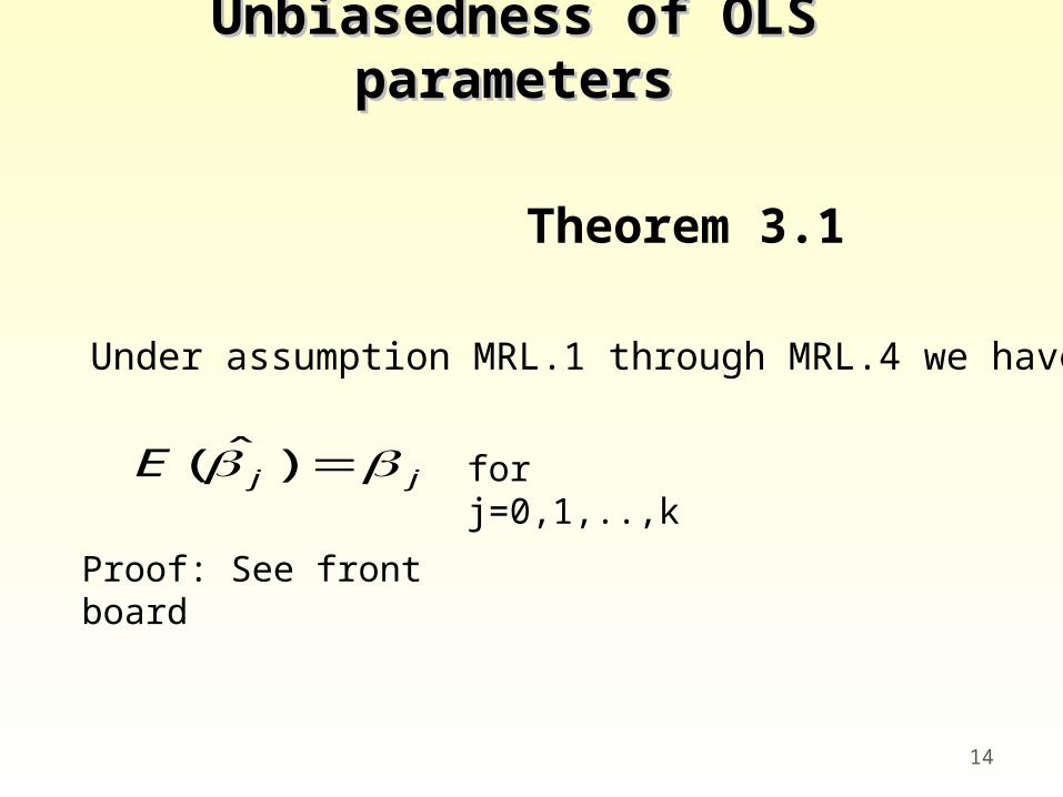
Unbiasedness of OLS Unbiasedness of OLS parametersparameters

Theorem 3.1

Under assumption MRL.1 through MRL.4 we have

jjE )ˆ( for j=0,1,..,k

Proof: See front board

15

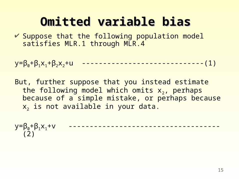
Omitted variable biasOmitted variable bias Suppose that the following population model

satisfies MLR.1 through MLR.4

y=β0+β1x1+β2x2+u -----------------------------(1)

But, further suppose that you instead estimate the following model which omits x2, perhaps because of a simple mistake, or perhaps because x2 is not available in your data.

y=β0+β1x1+v ------------------------------------(2)

16

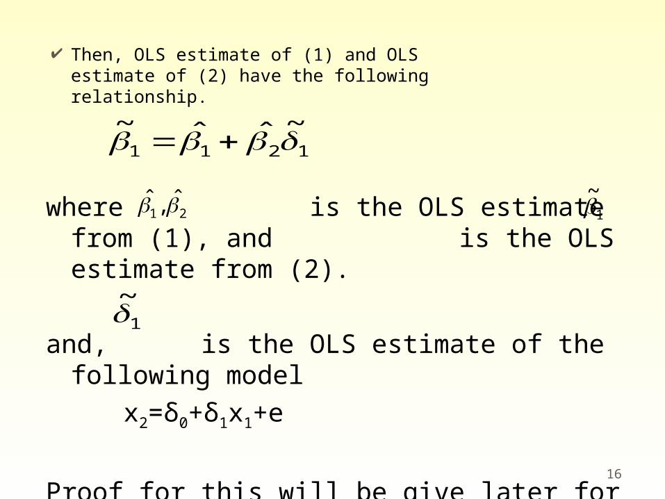
Then, OLS estimate of (1) and OLS estimate of (2) have the following relationship.

21ˆ,ˆ where is the OLS estimate from (1),

and is the OLS estimate from (2).

and, is the OLS estimate of the following model

x2=δ0+δ1x1+e

Proof for this will be give later for a general case.

1

~

1211

~ˆˆ~

1

~

17

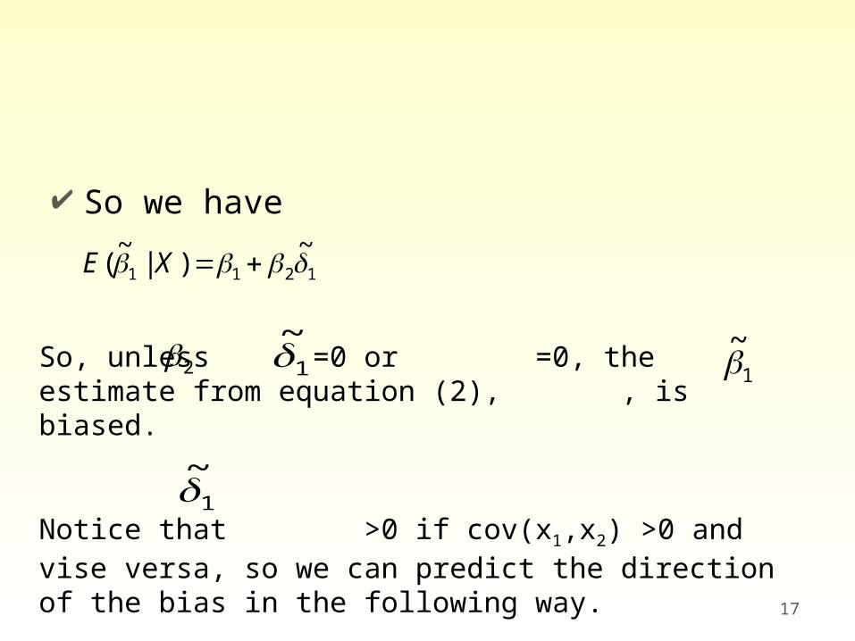
So we have

1211

~)|

~( XE

So, unless =0 or =0, the estimate from equation (2), , is biased.

Notice that >0 if cov(x1,x2) >0 and vise versa, so we can predict the direction of the bias in the following way.

2 1

~

1

~

1

~

18

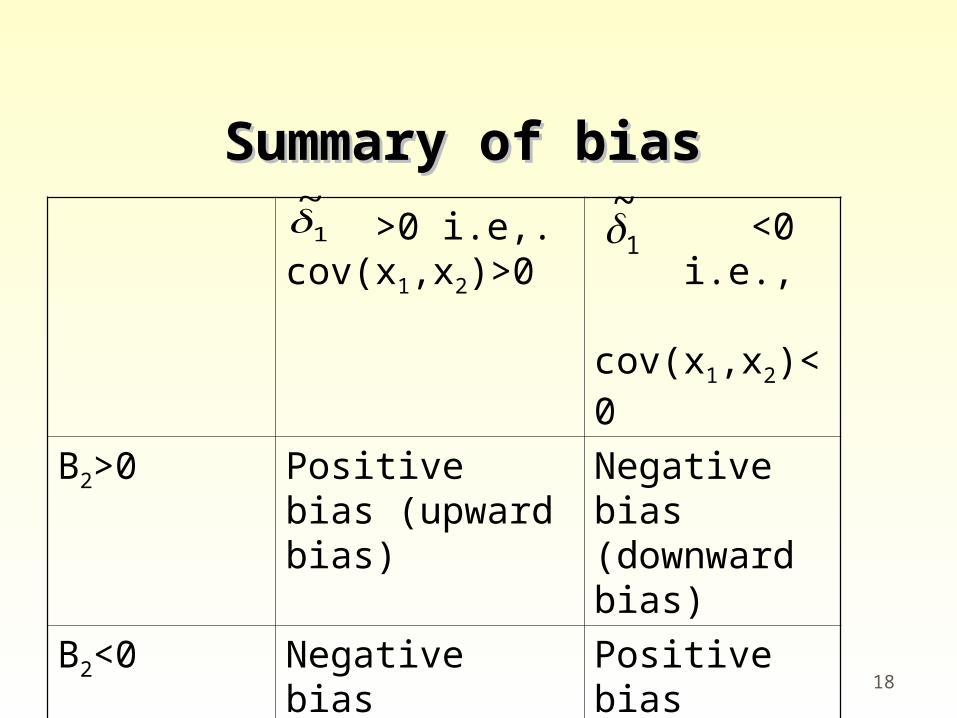
Summary of biasSummary of bias

>0 i.e,. cov(x1,x2)>0

<0 i.e., cov(x1,x2)<0

Β2>0 Positive bias (upward bias)

Negative bias (downward bias)

Β2<0 Negative bias (downward bias)

Positive bias (upward bias)

1

~1

~

19

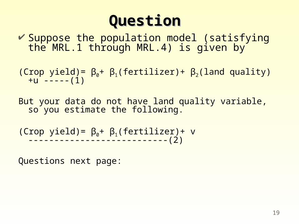
QuestionQuestion Suppose the population model (satisfying the

MRL.1 through MRL.4) is given by

(Crop yield)= β0+ β1(fertilizer)+ β2(land quality)+u -----(1)

But your data do not have land quality variable, so you estimate the following.

(Crop yield)= β0+ β1(fertilizer)+ v ---------------------------(2)

Questions next page:

20

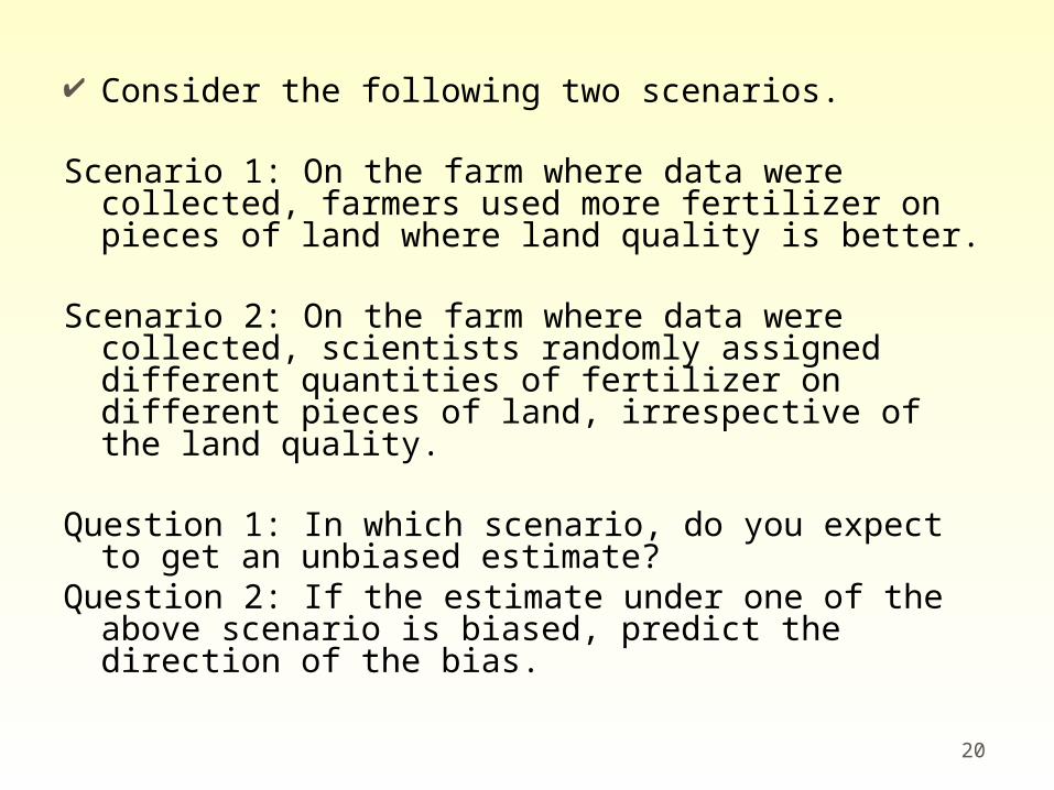
Consider the following two scenarios.

Scenario 1: On the farm where data were collected, farmers used more fertilizer on pieces of land where land quality is better.

Scenario 2: On the farm where data were collected, scientists randomly assigned different quantities of fertilizer on different pieces of land, irrespective of the land quality.

Question 1: In which scenario, do you expect to get an unbiased estimate?

Question 2: If the estimate under one of the above scenario is biased, predict the direction of the bias.

21

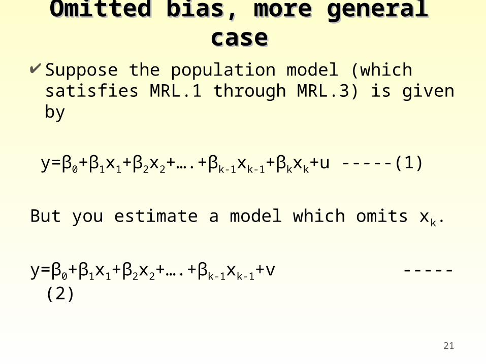
Omitted bias, more general Omitted bias, more general casecase

Suppose the population model (which satisfies MRL.1 through MRL.3) is given by

y=β0+β1x1+β2x2+….+βk-1xk-1+βkxk+u -----(1)

But you estimate a model which omits xk.

y=β0+β1x1+β2x2+….+βk-1xk-1+v -----(2)

22

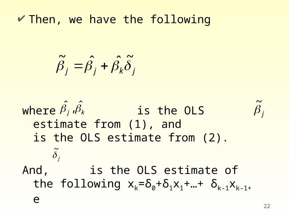
Then, we have the following

jkjj ~ˆˆ~

where is the OLS estimate from (1), and is the OLS estimate from (2).

And, is the OLS estimate of the following xk=δ0+δ1x1+…+ δk-1xk-1+ e

j~

kj ˆ,ˆj~

23

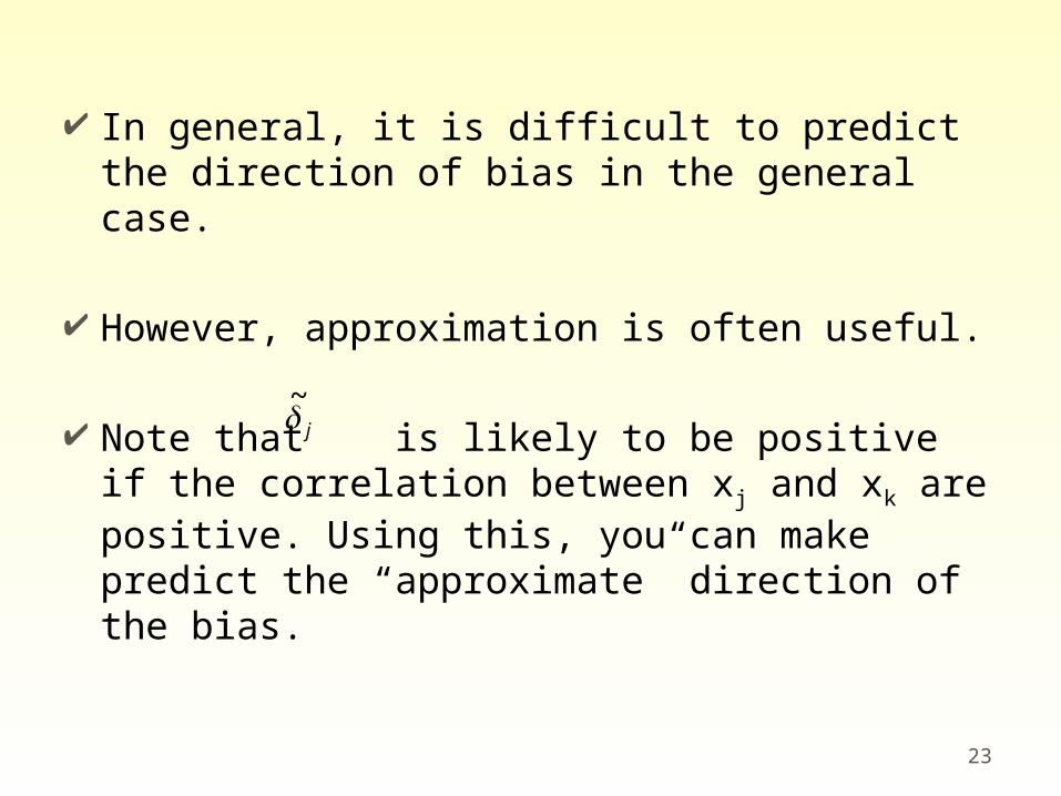
In general, it is difficult to predict the direction of bias in the general case.

However, approximation is often useful.

Note that is likely to be positive if the correlation between xj and xk are positive. Using this, you can make predict the “approximate” direction of the bias.

j~

24

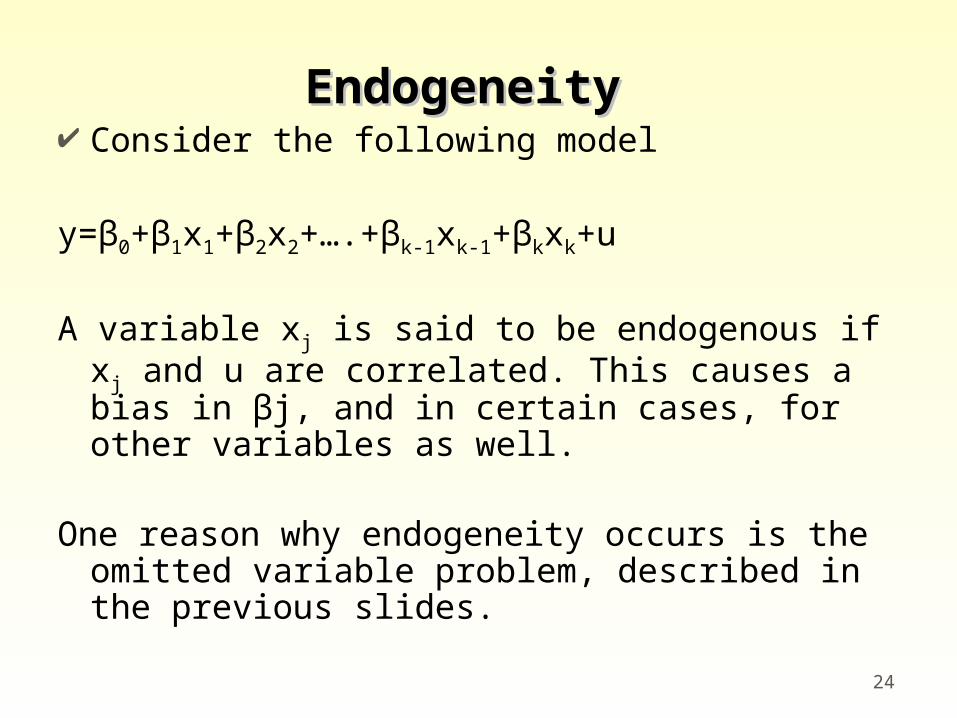
EndogeneityEndogeneity Consider the following model

y=β0+β1x1+β2x2+….+βk-1xk-1+βkxk+u

A variable xj is said to be endogenous if xj and u are correlated. This causes a bias in βj, and in certain cases, for other variables as well.

One reason why endogeneity occurs is the omitted variable problem, described in the previous slides.

25

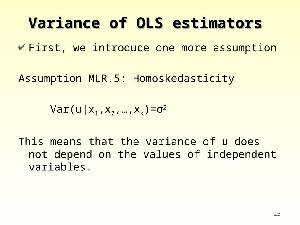
Variance of OLS estimatorsVariance of OLS estimators

First, we introduce one more assumption

Assumption MLR.5: Homoskedasticity

Var(u|x1,x2,…,xk)=σ2

This means that the variance of u does not depend on the values of independent variables.

26

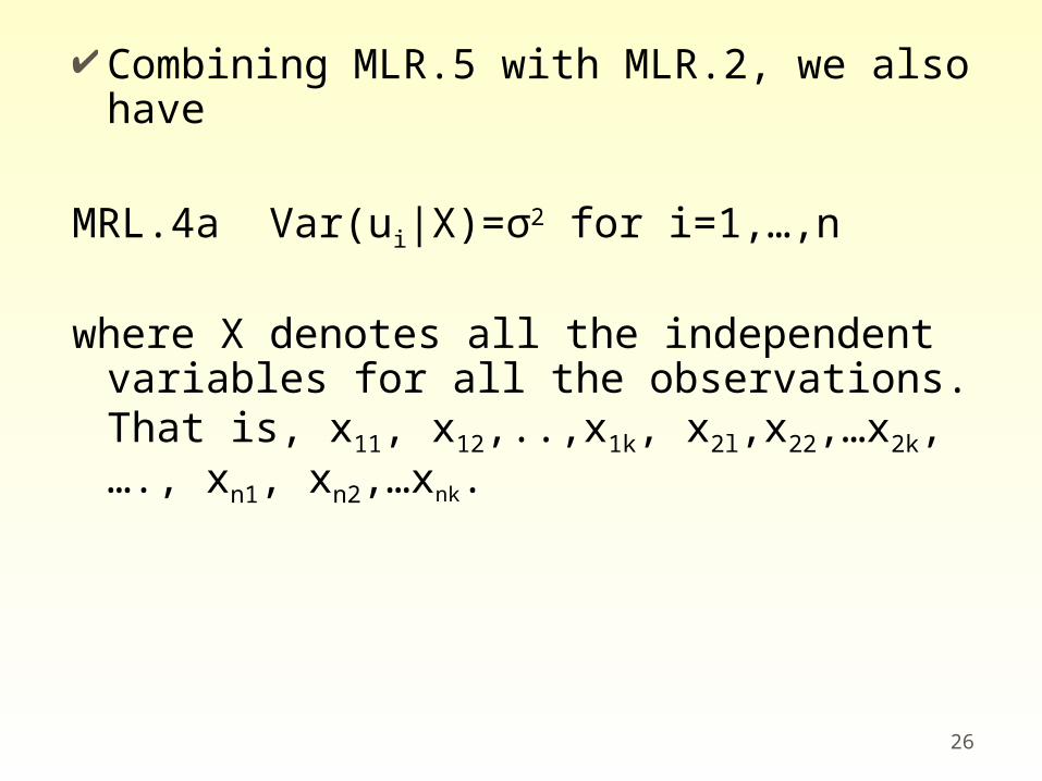
Combining MLR.5 with MLR.2, we also have

MRL.4a Var(ui|X)=σ2 for i=1,…,n

where X denotes all the independent variables for all the observations. That is, x11, x12,..,x1k, x2l,x22,…x2k,…., xn1, xn2,…xnk.

27

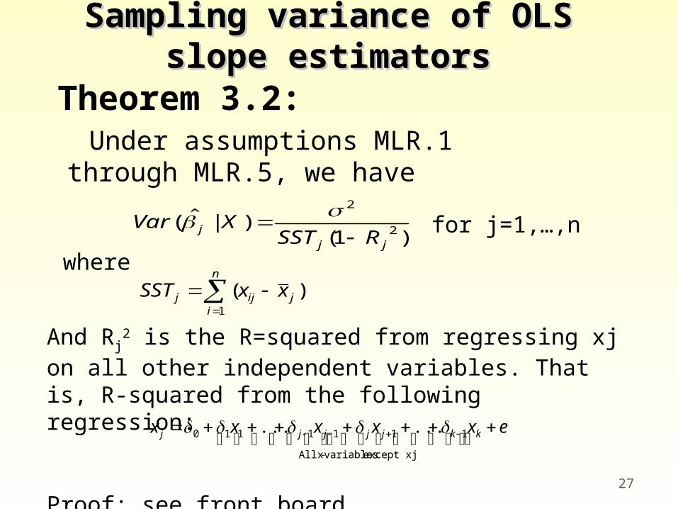
Sampling variance of OLS Sampling variance of OLS slope estimatorsslope estimators

Theorem 3.2: Under assumptions MLR.1 through

MLR.5, we have

)1()|ˆ( 2

2

jj

jRSST

XVar

)(1

n

ijijj xxSST

where

And Rj2 is the R=squared from regressing xj on all other

independent variables. That is, R-squared from the following regression:

Proof: see front board

for j=1,…,n

exxxxx kkjjjjj except xj variables- xAll

1111110 ......

28

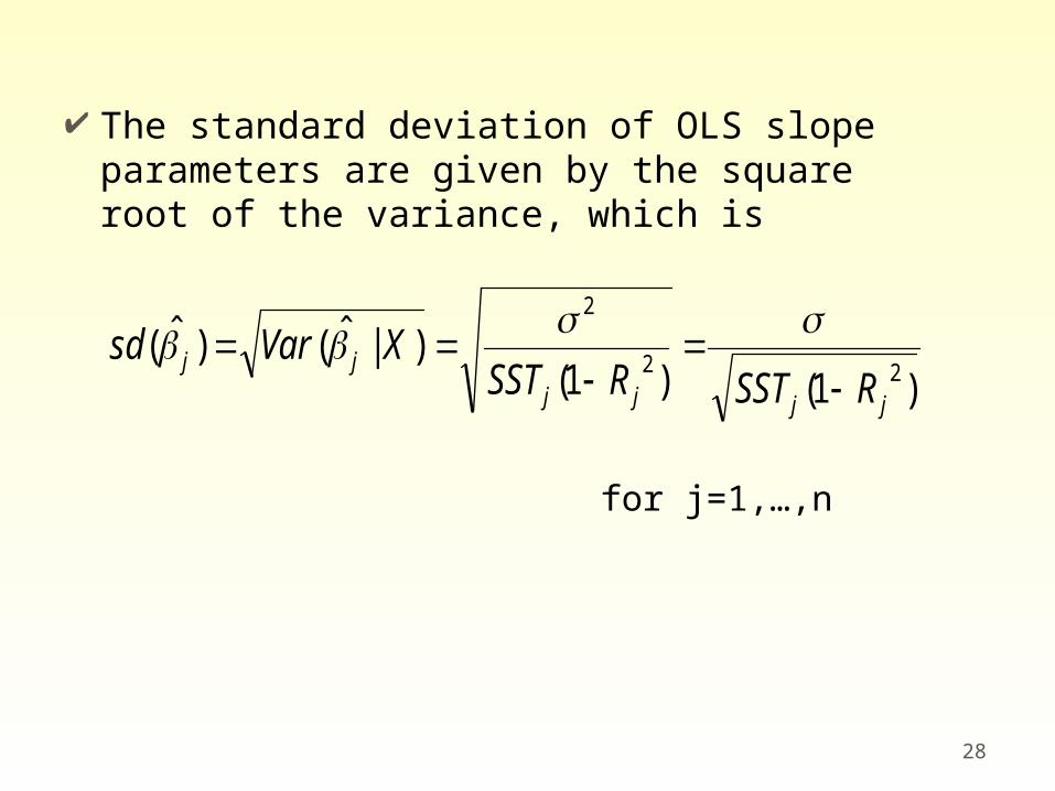
The standard deviation of OLS slope parameters are given by the square root of the variance, which is

)1()1()|ˆ()ˆ(

22

2

jjjj

jjRSSTRSST

XVarsd

for j=1,…,n

29

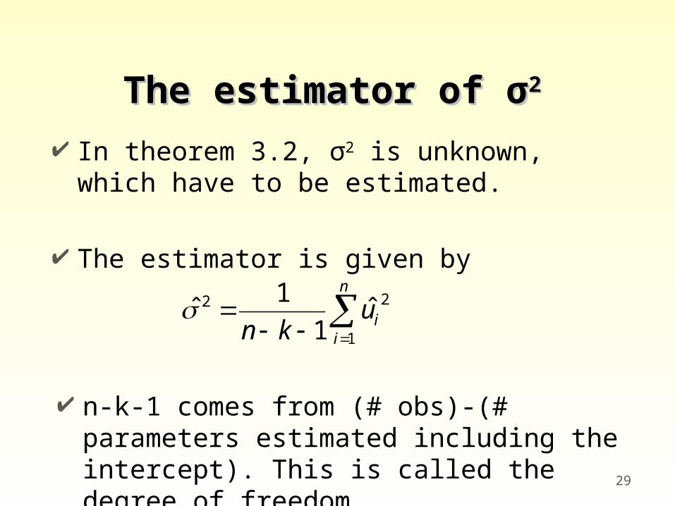
In theorem 3.2, σ2 is unknown, which have to be estimated.

The estimator is given by

n

iiukn 1

22 ˆ1

1

n-k-1 comes from (# obs)-(# parameters estimated including the intercept). This is called the degree of freedom.

The estimator of The estimator of σσ22

30

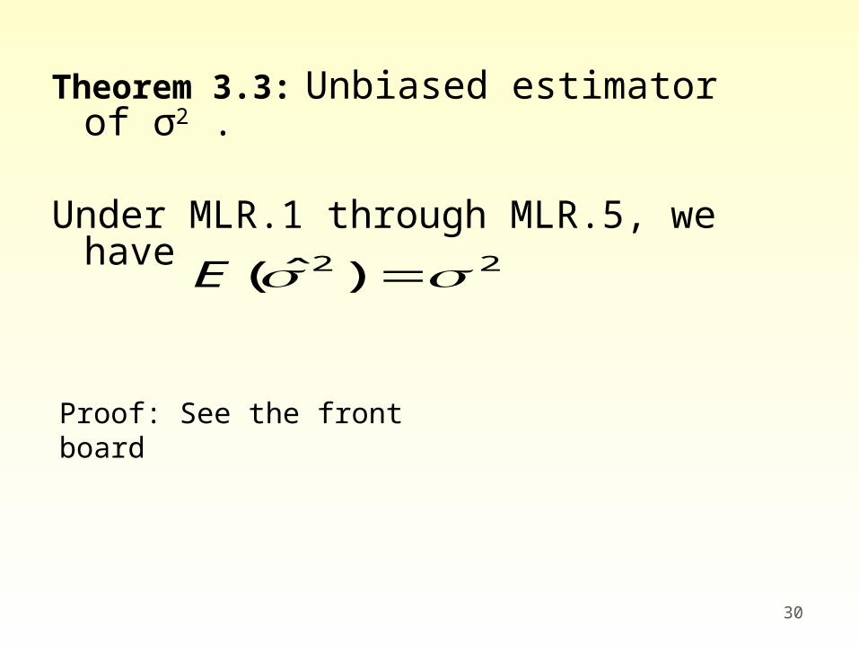
Theorem 3.3: Unbiased estimator of σ2 .

Under MLR.1 through MLR.5, we have 22 )ˆ( E

Proof: See the front board

31

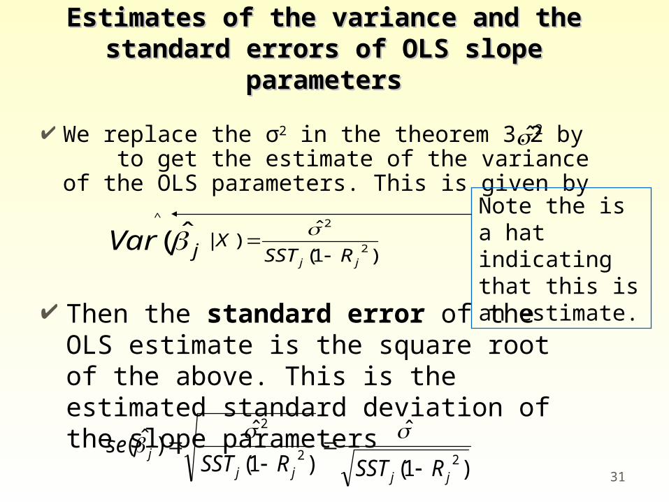
Estimates of the variance and the Estimates of the variance and the standard errors of OLS slope standard errors of OLS slope

parametersparameters

We replace the σ2 in the theorem 3.2 by to get the estimate of the variance of the OLS parameters. This is given by

)1(

ˆ)| 2

2^

ˆ(jj RSST

XjVar

Note the is a hat indicating that this is an estimate.

Then the standard error of the OLS estimate is the square root of the above. This is the estimated standard deviation of the slope parameters

)1(

ˆ

)1(

ˆ)ˆ(

22

2

jjjj

jRSSTRSST

se

2

32

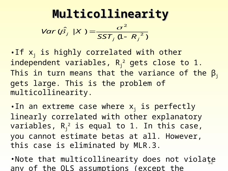
MulticollinearityMulticollinearity

)1()|ˆ( 2

2

jj

jRSST

XVar

•If xj is highly correlated with other independent variables, Rj2 gets

close to 1. This in turn means that the variance of the βj gets large. This is the problem of multicollinearity.

•In an extreme case where xj is perfectly linearly correlated with other explanatory variables, Rj

2 is equal to 1. In this case, you cannot estimate betas at all. However, this case is eliminated by MLR.3.

•Note that multicollinearity does not violate any of the OLS assumptions (except the perfect multicollinearity case), and should not be over-emphasized. You can reduce variance by increasing the number of observations.

33

Gauss-Markov theoremGauss-Markov theoremTheorem 3.4

Under Assumption MLR.1 through MRL.5, OLS estimates of beta parameters are the best linear unbiased estimators.

This theorem means that among all the possible unbiased estimators of the beta parameters, OLS estimators have the smallest variances.