Corresponds to Chapter 11 of Tamhane & Dunlop · 2019-04-11 · Multiple Linear Regression...
45
Multiple Linear Regression Corresponds to Chapter 11 of Tamhane & Dunlop Slides prepared by Elizabeth Newton (MIT) with some slides by Roy Welsch (MIT).
Transcript of Corresponds to Chapter 11 of Tamhane & Dunlop · 2019-04-11 · Multiple Linear Regression...
Multiple Linear Regression
Corresponds to Chapter 11 ofTamhane & Dunlop
Slides prepared by Elizabeth Newton (MIT)with some slides by Roy Welsch (MIT).
Linear Regression
Review:Linear Model: y=Xβ + ε
y~N(Xβ, σ2I)Least squares: =(X’X)X’y
= fitted value of y = X =X(X’X)-1X’y=Hy
e = error = residuals = y- = y-Hy=(I-H)y
βy
y
β
2

Properties of the Hat matrix
• Symmetric: H’=H• Idempotent: HH=H• Trace(H) = sum(diag(H)) = k+1 = number of
columns in the X matrix• 1’H=vector of 1’s (hence y and have same
mean)• 1’(I-H) = vector of 0’s (hence mean of residuals
is 0).• What is H when X is only a column of 1’s?
y
3
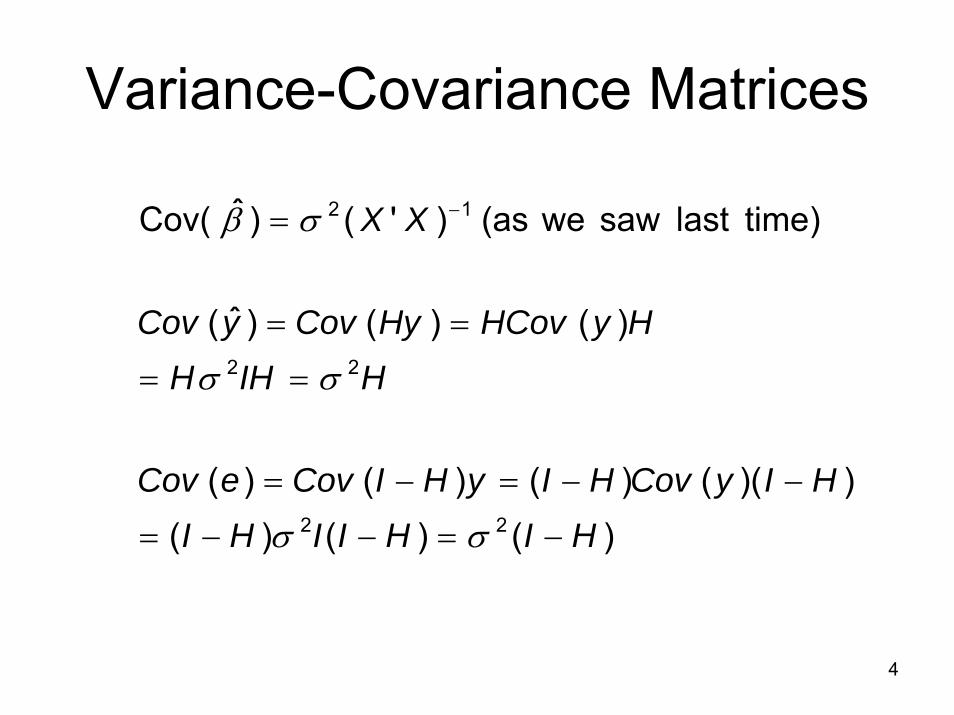
Variance-Covariance Matrices
)()()())(()()()(
)()()ˆ(
time) lastsaw we(as )'()ˆCov(
22
22
12
HIHIIHIHIyCovHIyHICoveCov
HIHHHyHCovHyCovyCov
XX
−=−−=
−−=−=
==
==
= −
σσ
σσ
σβ
4
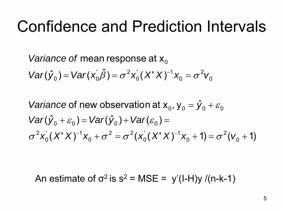
Confidence and Prediction Intervals
)1()1)'(()'()()ˆ()ˆ(
ˆ y, xat nobservationew of
)'()ˆ()ˆ(
xat response mean
02
01'
022
01'
02
0000
0000
02
01'
02'
00
0
+=+=+
=+=+
+=
===
−−
−
vxXXxxXXx
VaryVaryVaryVariance
vxXXxxVaryVar
ofVariance
σσσσ
εεε
σσβ
An estimate of σ2 is s2 = MSE = y’(I-H)y /(n-k-1)
5
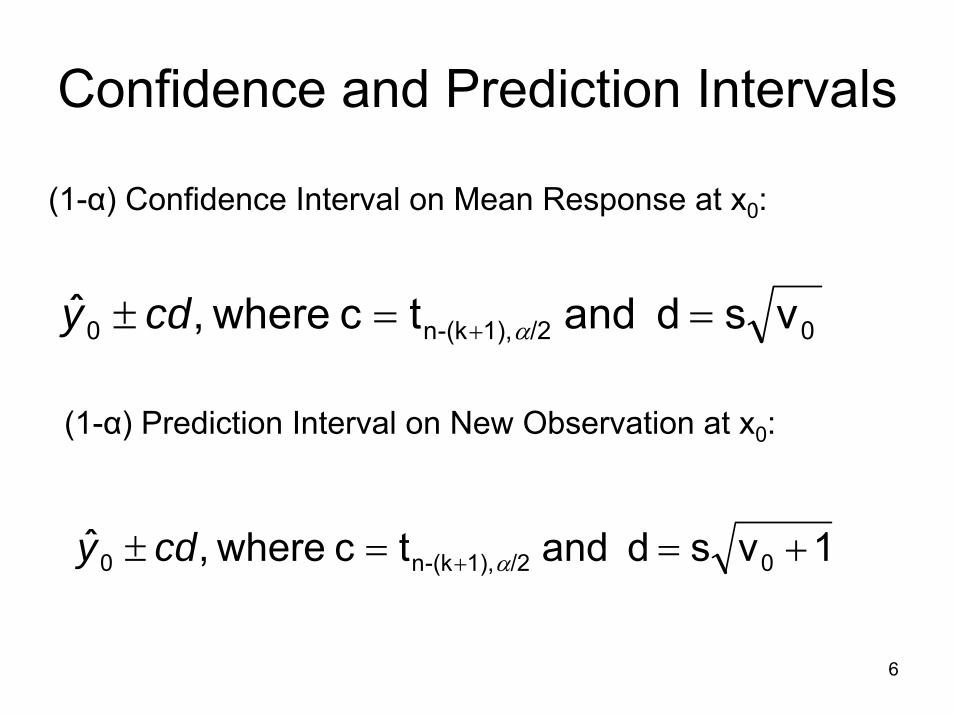
Confidence and Prediction Intervals
(1-α) Confidence Interval on Mean Response at x0:
0/2 1),(k-n0 vsd and tc where,ˆ ==± + αcdy
(1-α) Prediction Interval on New Observation at x0:
1vsd and tc where,ˆ 0/2 1),(k-n0 +==± + αcdy
6
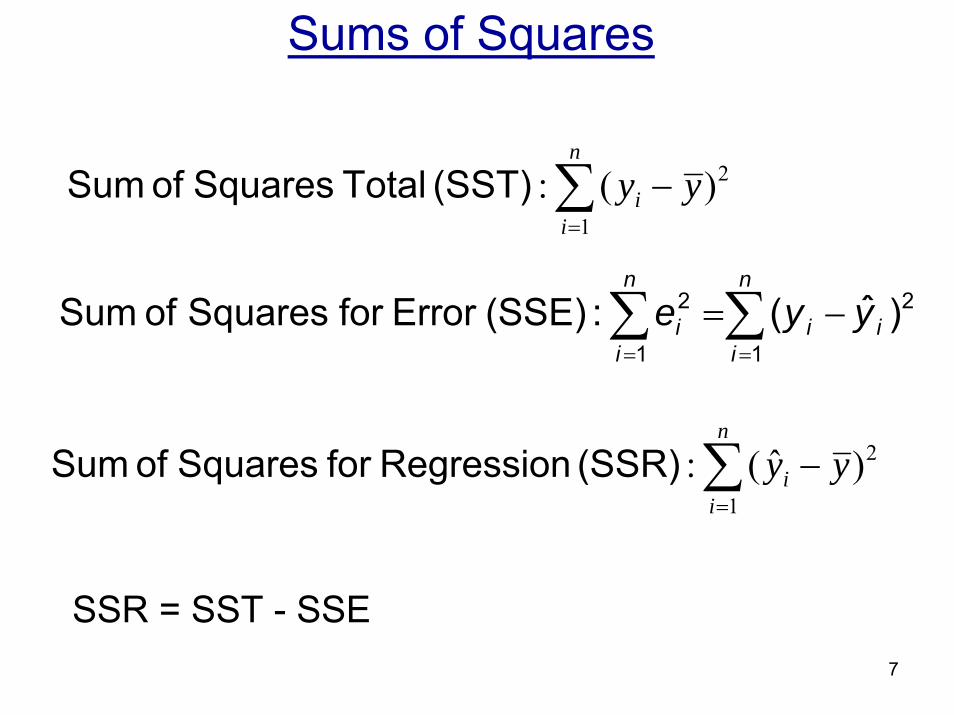
Sums of Squares
∑=
−n
ii yy
1
2)(: (SST) Total Squares of Sum
∑∑==
−=n
iii
n
ii yye
1
2
1
2 )ˆ(: (SSE) Error for Squares of Sum
∑=
−n
ii yy
1
2)ˆ(: (SSR) Regression for Squares of Sum
SSR = SST - SSE7
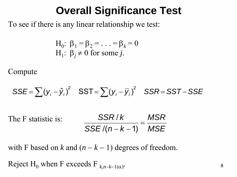
Overall Significance TestTo see if there is any linear relationship we test:
H0: β1 = β2 = . . . = βk = 0H1: βj ≠ 0 for some j.
Compute
The F statistic is:
with F based on k and (n − k − 1) degrees of freedom.
Reject H0 when F exceeds F k,n−k−1(α).
SSESSTSSRyyyySSE iiii −=−=−= ∑∑ )(SST )ˆ( 22
MSEMSR
knSSEkSSR
=−− )1/(
/
8
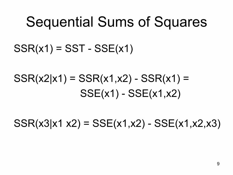
Sequential Sums of Squares
SSR(x1) = SST - SSE(x1)
SSR(x2|x1) = SSR(x1,x2) - SSR(x1) =SSE(x1) - SSE(x1,x2)
SSR(x3|x1 x2) = SSE(x1,x2) - SSE(x1,x2,x3)
9
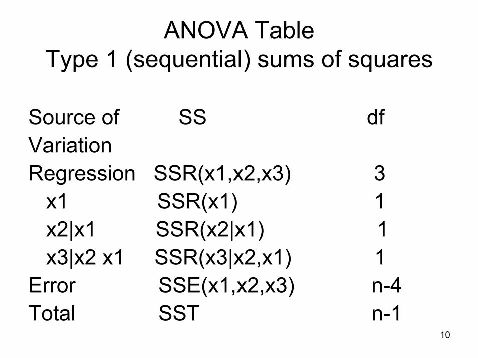
ANOVA TableType 1 (sequential) sums of squares
Source of SS dfVariationRegression SSR(x1,x2,x3) 3
x1 SSR(x1) 1x2|x1 SSR(x2|x1) 1x3|x2 x1 SSR(x3|x2,x1) 1
Error SSE(x1,x2,x3) n-4Total SST n-1
10
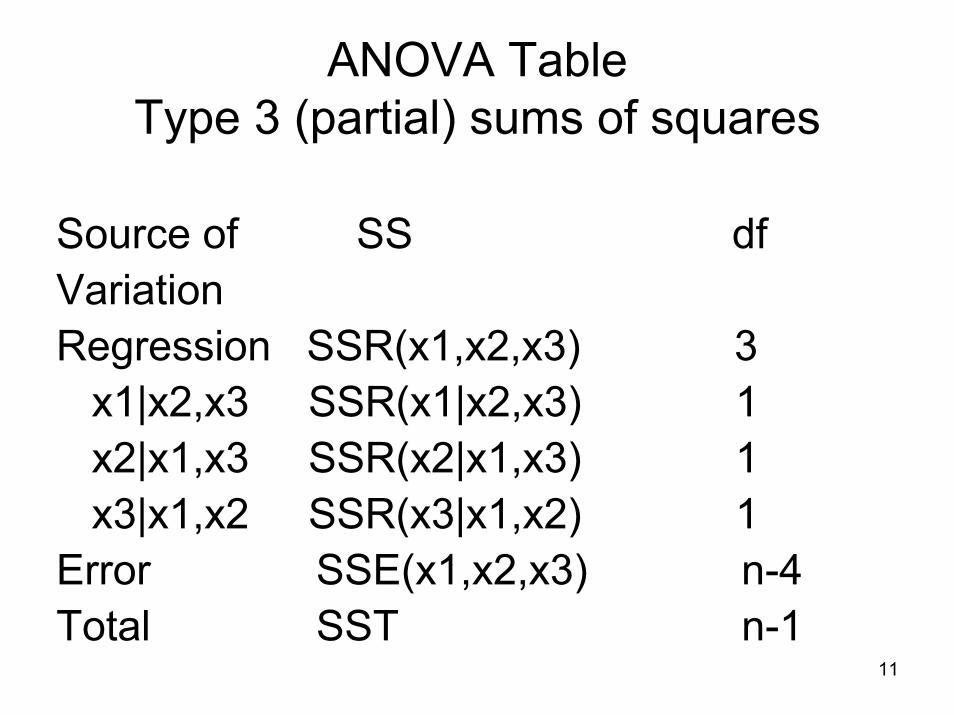
ANOVA TableType 3 (partial) sums of squares
Source of SS dfVariationRegression SSR(x1,x2,x3) 3
x1|x2,x3 SSR(x1|x2,x3) 1x2|x1,x3 SSR(x2|x1,x3) 1x3|x1,x2 SSR(x3|x1,x2) 1
Error SSE(x1,x2,x3) n-4Total SST n-1
11
12
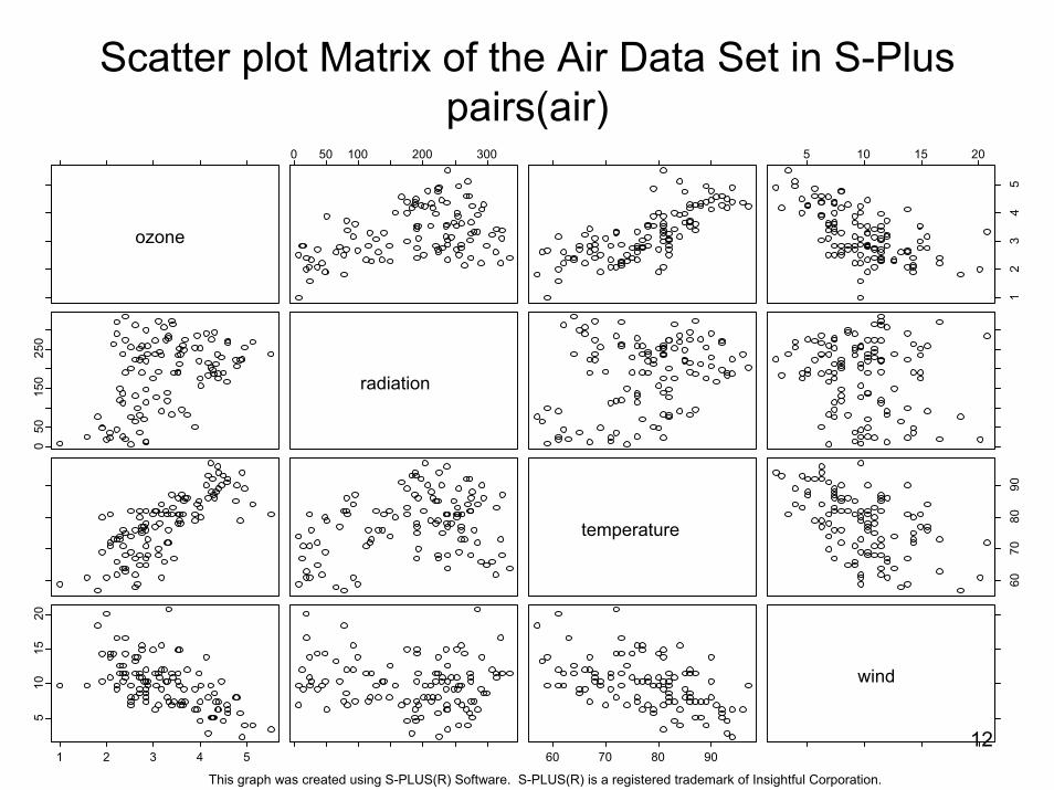
Scatter plot Matrix of the Air Data Set in S-Plus pairs(air)
ozone
0 50 100 200 300 5 10 15 20
12
34
5
050
150
250
radiation
temperature
6070
8090
1 2 3 4 5
510
1520
60 70 80 90
wind
This graph was created using S-PLUS(R) Software. S-PLUS(R) is a registered trademark of Insightful Corporation.
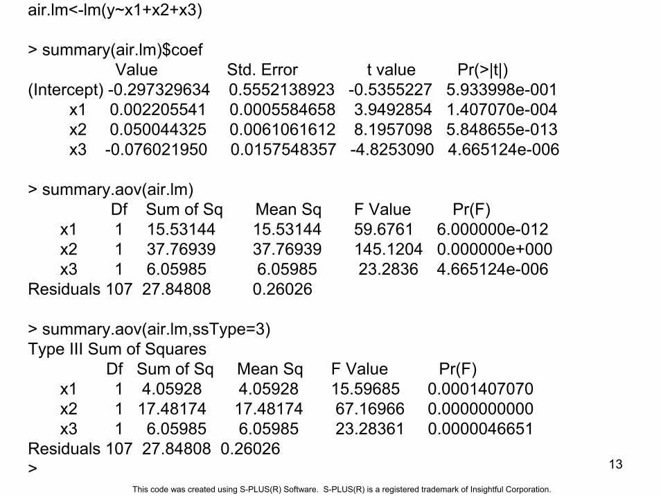
air.lm<-lm(y~x1+x2+x3)
> summary(air.lm)$coefValue Std. Error t value Pr(>|t|)
(Intercept) -0.297329634 0.5552138923 -0.5355227 5.933998e-001x1 0.002205541 0.0005584658 3.9492854 1.407070e-004x2 0.050044325 0.0061061612 8.1957098 5.848655e-013x3 -0.076021950 0.0157548357 -4.8253090 4.665124e-006
> summary.aov(air.lm)Df Sum of Sq Mean Sq F Value Pr(F)
x1 1 15.53144 15.53144 59.6761 6.000000e-012x2 1 37.76939 37.76939 145.1204 0.000000e+000x3 1 6.05985 6.05985 23.2836 4.665124e-006
Residuals 107 27.84808 0.26026
> summary.aov(air.lm,ssType=3)Type III Sum of Squares
Df Sum of Sq Mean Sq F Value Pr(F) x1 1 4.05928 4.05928 15.59685 0.0001407070x2 1 17.48174 17.48174 67.16966 0.0000000000x3 1 6.05985 6.05985 23.28361 0.0000046651
Residuals 107 27.84808 0.26026 > 13
This code was created using S-PLUS(R) Software. S-PLUS(R) is a registered trademark of Insightful Corporation.
Polynomial Models
y=β0 + β1x + β2x2 … + βkxk
Problems:Powers of x tend to be large in magnitudePowers of x tend to be highly correlated
Solutions:Centering and scaling of x variablesOrthogonal polynomials (poly(x,k) in S-Plus,
see Seber for methods of generating)
14
15
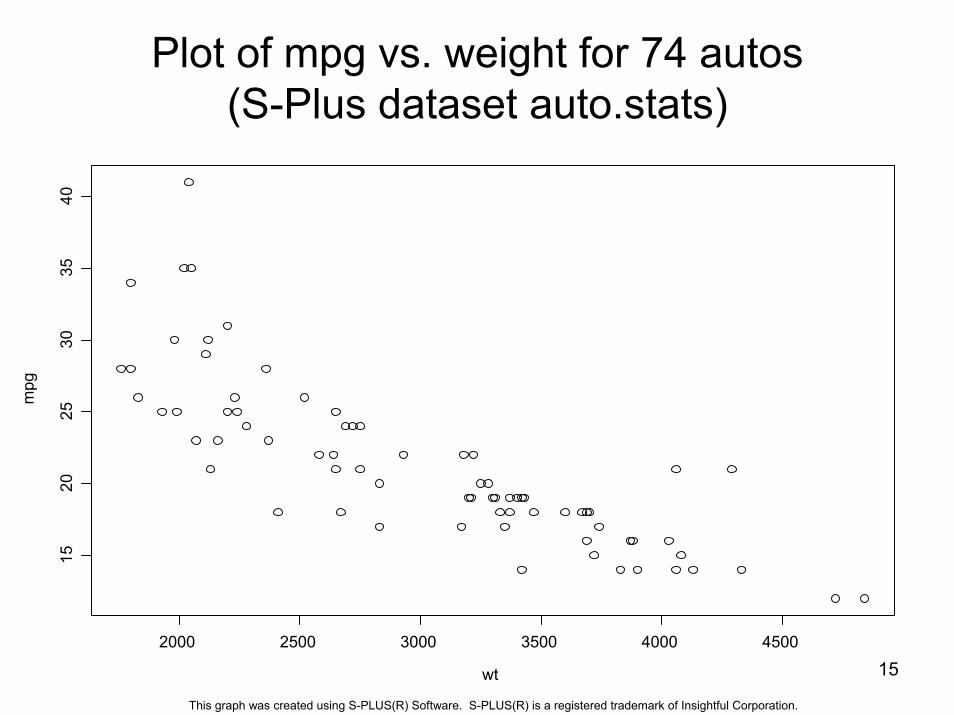
Plot of mpg vs. weight for 74 autos(S-Plus dataset auto.stats)
wt
mpg
2000 2500 3000 3500 4000 4500
1520
2530
3540
This graph was created using S-PLUS(R) Software. S-PLUS(R) is a registered trademark of Insightful Corporation.
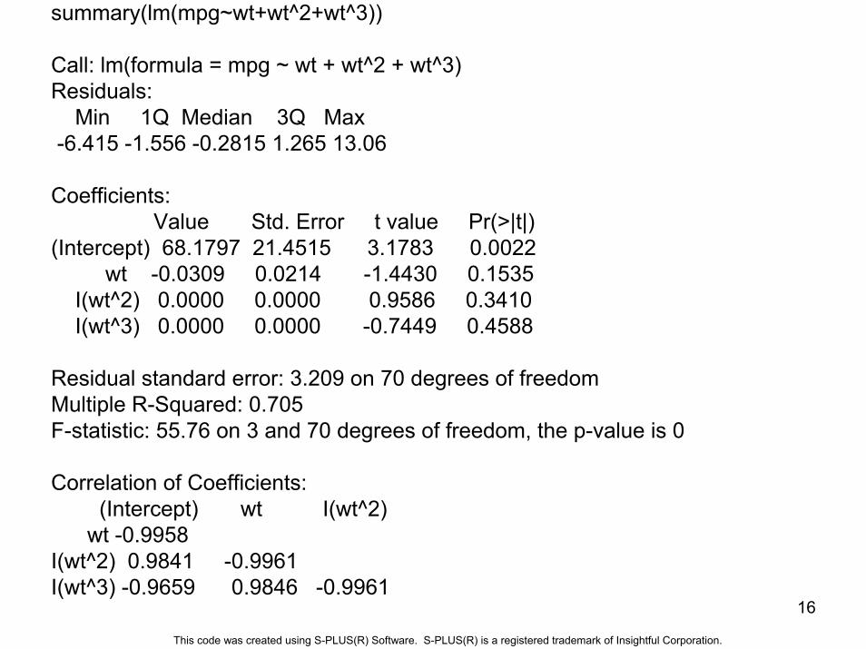
summary(lm(mpg~wt+wt^2+wt^3))
Call: lm(formula = mpg ~ wt + wt^2 + wt^3)Residuals:
Min 1Q Median 3Q Max -6.415 -1.556 -0.2815 1.265 13.06
Coefficients:Value Std. Error t value Pr(>|t|)
(Intercept) 68.1797 21.4515 3.1783 0.0022wt -0.0309 0.0214 -1.4430 0.1535
I(wt^2) 0.0000 0.0000 0.9586 0.3410I(wt^3) 0.0000 0.0000 -0.7449 0.4588
Residual standard error: 3.209 on 70 degrees of freedomMultiple R-Squared: 0.705 F-statistic: 55.76 on 3 and 70 degrees of freedom, the p-value is 0
Correlation of Coefficients:(Intercept) wt I(wt^2)
wt -0.9958 I(wt^2) 0.9841 -0.9961 I(wt^3) -0.9659 0.9846 -0.9961
16
This code was created using S-PLUS(R) Software. S-PLUS(R) is a registered trademark of Insightful Corporation.
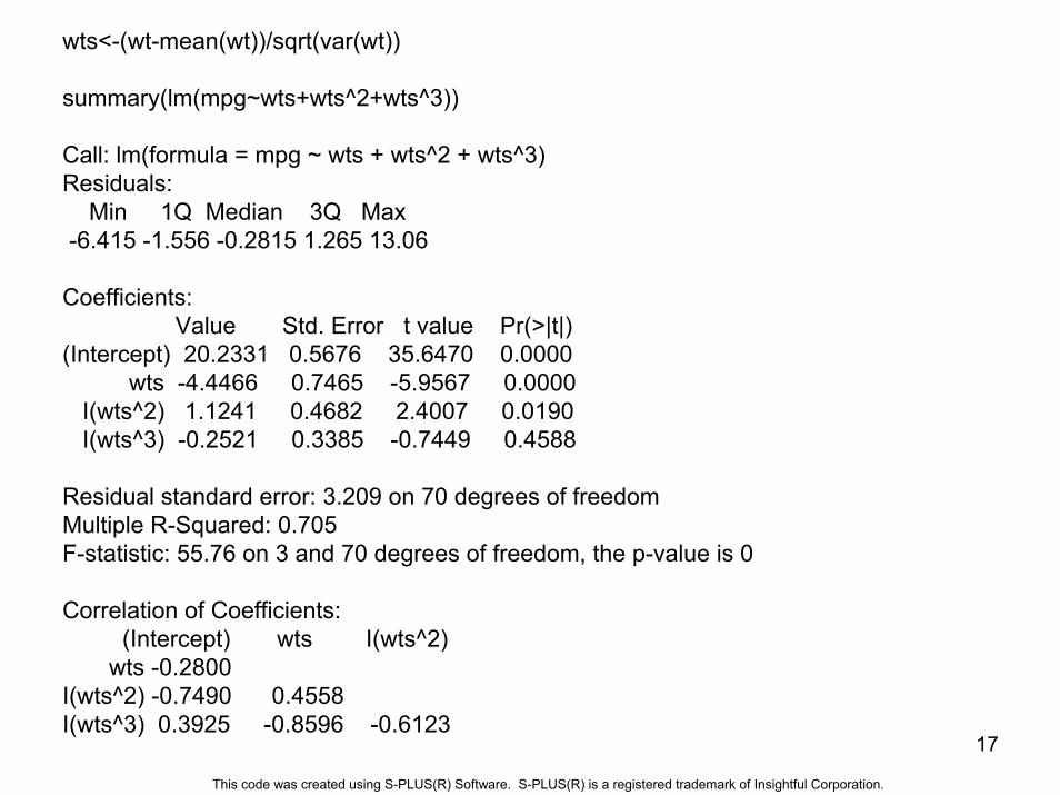
wts<-(wt-mean(wt))/sqrt(var(wt))
summary(lm(mpg~wts+wts^2+wts^3))
Call: lm(formula = mpg ~ wts + wts^2 + wts^3)Residuals:
Min 1Q Median 3Q Max -6.415 -1.556 -0.2815 1.265 13.06
Coefficients:Value Std. Error t value Pr(>|t|)
(Intercept) 20.2331 0.5676 35.6470 0.0000wts -4.4466 0.7465 -5.9567 0.0000
I(wts^2) 1.1241 0.4682 2.4007 0.0190I(wts^3) -0.2521 0.3385 -0.7449 0.4588
Residual standard error: 3.209 on 70 degrees of freedomMultiple R-Squared: 0.705 F-statistic: 55.76 on 3 and 70 degrees of freedom, the p-value is 0
Correlation of Coefficients:(Intercept) wts I(wts^2)
wts -0.2800 I(wts^2) -0.7490 0.4558 I(wts^3) 0.3925 -0.8596 -0.6123
17
This code was created using S-PLUS(R) Software. S-PLUS(R) is a registered trademark of Insightful Corporation.
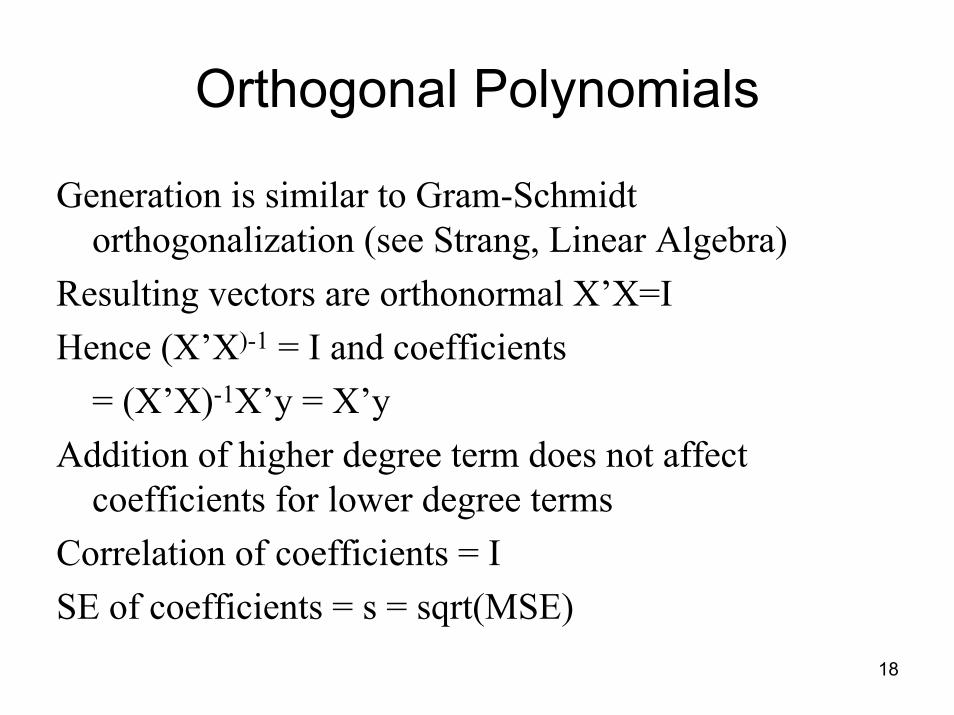
Orthogonal Polynomials
Generation is similar to Gram-Schmidt orthogonalization (see Strang, Linear Algebra)
Resulting vectors are orthonormal X’X=IHence (X’X)-1 = I and coefficients
= (X’X)-1X’y = X’yAddition of higher degree term does not affect
coefficients for lower degree termsCorrelation of coefficients = ISE of coefficients = s = sqrt(MSE)
18
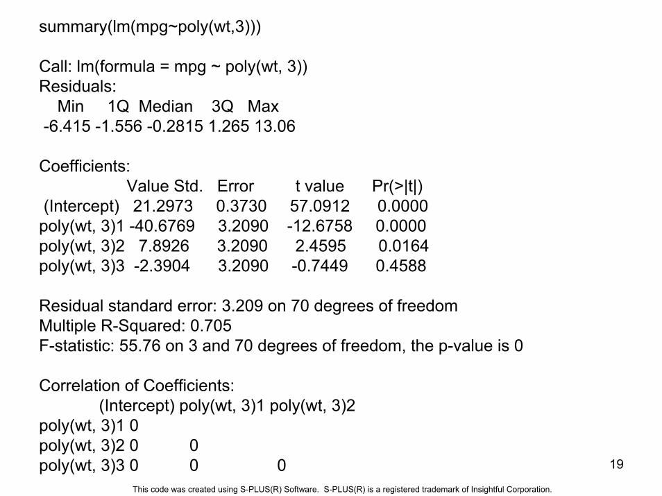
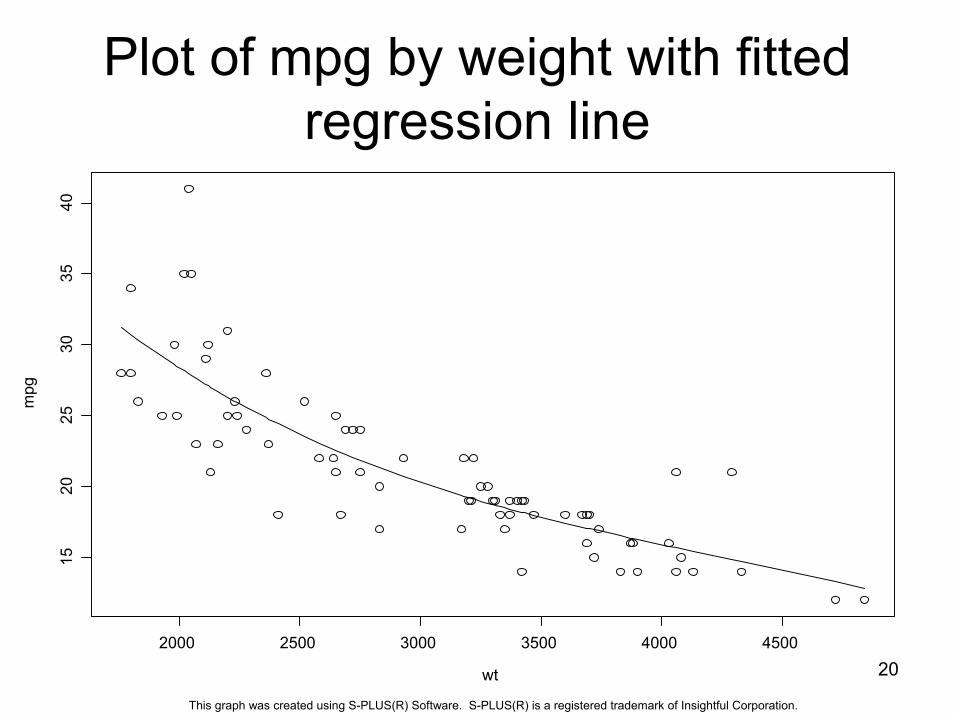
summary(lm(mpg~poly(wt,3)))
Call: lm(formula = mpg ~ poly(wt, 3))Residuals:
Min 1Q Median 3Q Max -6.415 -1.556 -0.2815 1.265 13.06
Coefficients:Value Std. Error t value Pr(>|t|)
(Intercept) 21.2973 0.3730 57.0912 0.0000poly(wt, 3)1 -40.6769 3.2090 -12.6758 0.0000poly(wt, 3)2 7.8926 3.2090 2.4595 0.0164poly(wt, 3)3 -2.3904 3.2090 -0.7449 0.4588
Residual standard error: 3.209 on 70 degrees of freedomMultiple R-Squared: 0.705 F-statistic: 55.76 on 3 and 70 degrees of freedom, the p-value is 0
Correlation of Coefficients:(Intercept) poly(wt, 3)1 poly(wt, 3)2
poly(wt, 3)1 0 poly(wt, 3)2 0 0 poly(wt, 3)3 0 0 0 19
This code was created using S-PLUS(R) Software. S-PLUS(R) is a registered trademark of Insightful Corporation.
20
Plot of mpg by weight with fitted regression line
wt
mpg
2000 2500 3000 3500 4000 4500
1520
2530
3540
This graph was created using S-PLUS(R) Software. S-PLUS(R) is a registered trademark of Insightful Corporation.
Indicator Variables
• Sometimes we might want to fit a model with a categorical variable as a predictor. For instance, automobile price as a function of where the car is made (Germany, Japan, USA).
• If there are c categories, we need c-1 indicator (0,1) variables as predictors. For instance j=1 if car is made in Japan, 0 otherwise, u=1 if car is made in USA, 0 otherwise.
• If there are just 2 categories and no other predictors, we could just do a t-test for difference in means.
21
22
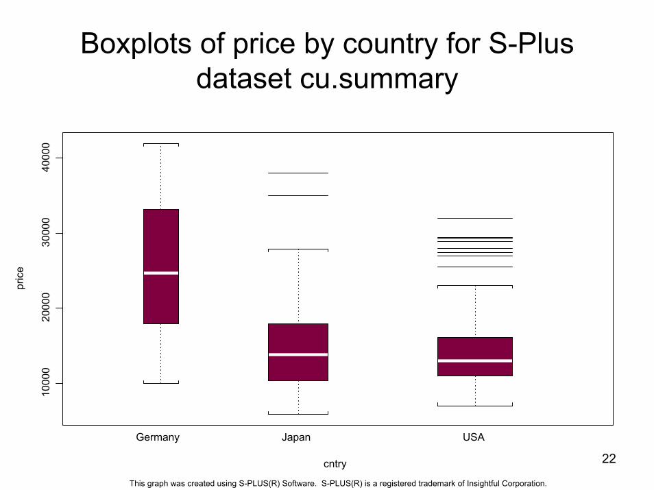
Boxplots of price by country for S-Plus dataset cu.summary
1000
020
000
3000
040
000
pric
e
Germany Japan USA
cntry
This graph was created using S-PLUS(R) Software. S-PLUS(R) is a registered trademark of Insightful Corporation.
23
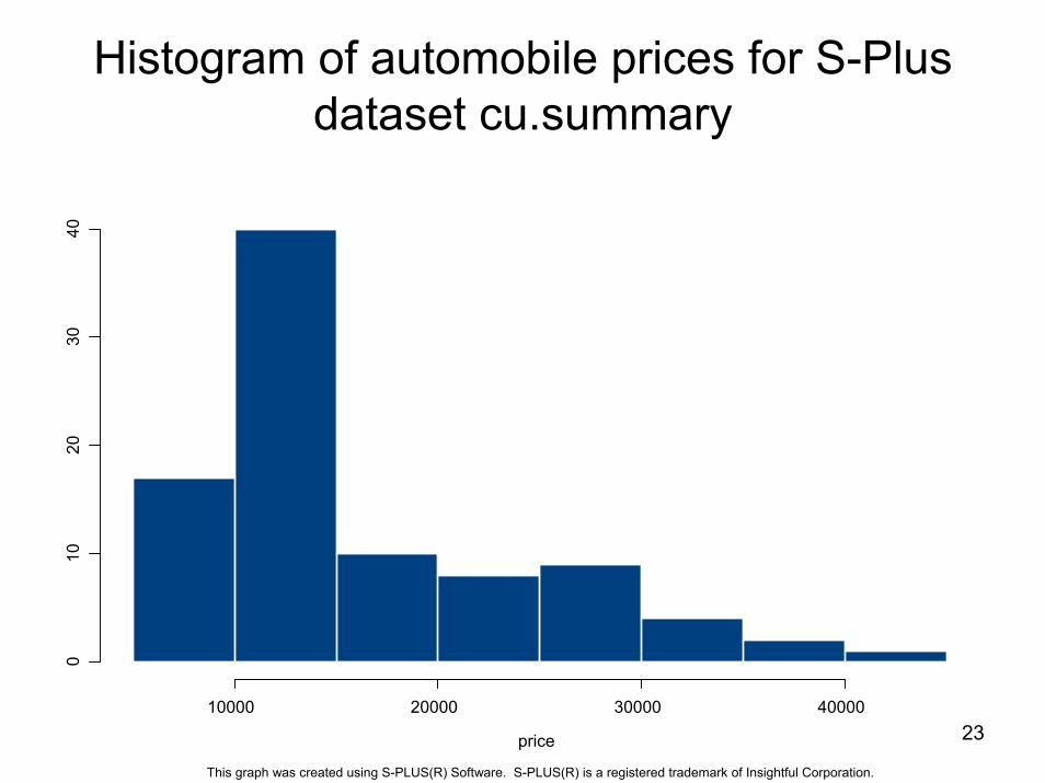
Histogram of automobile prices for S-Plus dataset cu.summary
10000 20000 30000 40000
010
2030
40
price
This graph was created using S-PLUS(R) Software. S-PLUS(R) is a registered trademark of Insightful Corporation.
24
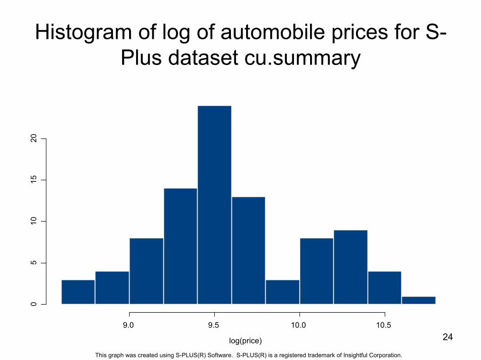
Histogram of log of automobile prices for S-Plus dataset cu.summary
9.0 9.5 10.0 10.5
05
1015
20
log(price)
This graph was created using S-PLUS(R) Software. S-PLUS(R) is a registered trademark of Insightful Corporation.
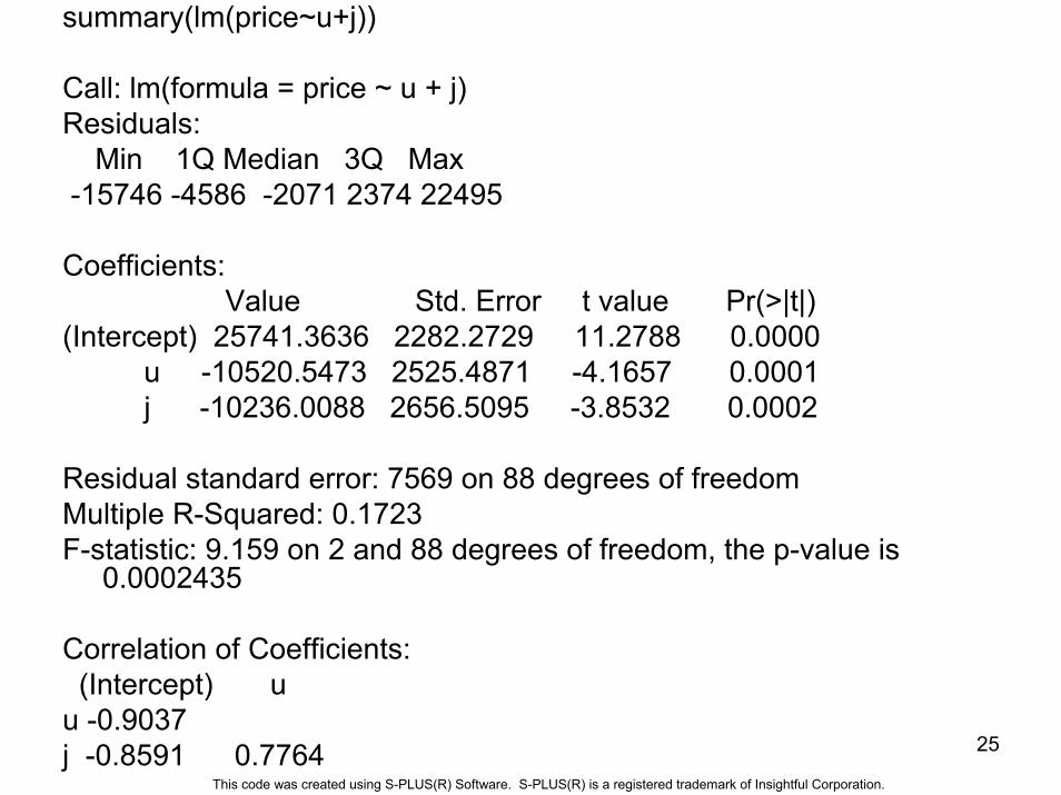
summary(lm(price~u+j))
Call: lm(formula = price ~ u + j)Residuals:
Min 1Q Median 3Q Max -15746 -4586 -2071 2374 22495
Coefficients:Value Std. Error t value Pr(>|t|)
(Intercept) 25741.3636 2282.2729 11.2788 0.0000u -10520.5473 2525.4871 -4.1657 0.0001j -10236.0088 2656.5095 -3.8532 0.0002
Residual standard error: 7569 on 88 degrees of freedomMultiple R-Squared: 0.1723 F-statistic: 9.159 on 2 and 88 degrees of freedom, the p-value is
0.0002435
Correlation of Coefficients:(Intercept) u
u -0.9037 j -0.8591 0.7764 25
This code was created using S-PLUS(R) Software. S-PLUS(R) is a registered trademark of Insightful Corporation.
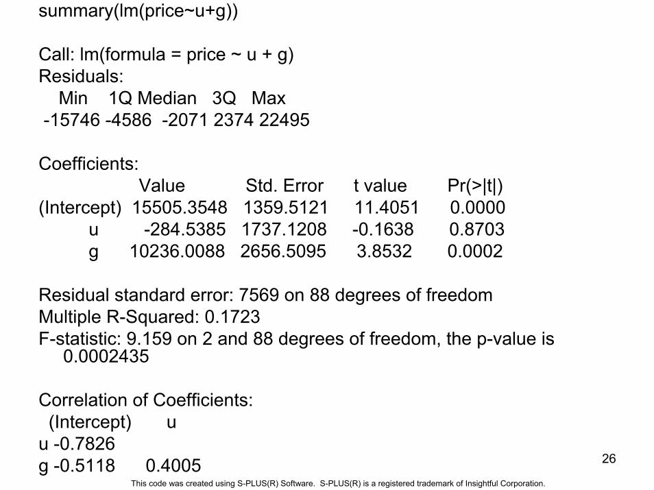
summary(lm(price~u+g))
Call: lm(formula = price ~ u + g)Residuals:
Min 1Q Median 3Q Max -15746 -4586 -2071 2374 22495
Coefficients:Value Std. Error t value Pr(>|t|)
(Intercept) 15505.3548 1359.5121 11.4051 0.0000u -284.5385 1737.1208 -0.1638 0.8703g 10236.0088 2656.5095 3.8532 0.0002
Residual standard error: 7569 on 88 degrees of freedomMultiple R-Squared: 0.1723 F-statistic: 9.159 on 2 and 88 degrees of freedom, the p-value is
0.0002435
Correlation of Coefficients:(Intercept) u
u -0.7826 g -0.5118 0.4005 26
This code was created using S-PLUS(R) Software. S-PLUS(R) is a registered trademark of Insightful Corporation.
Regression DiagnosticsGoal: identify remarkable observations and unremarkable
predictors.
Problems with observations:OutliersInfluential observations
Problems with predictors:A predictor may not add much to model.A predictor may be too similar to another predictor (collinearity).Predictors may have been left out.
27
28
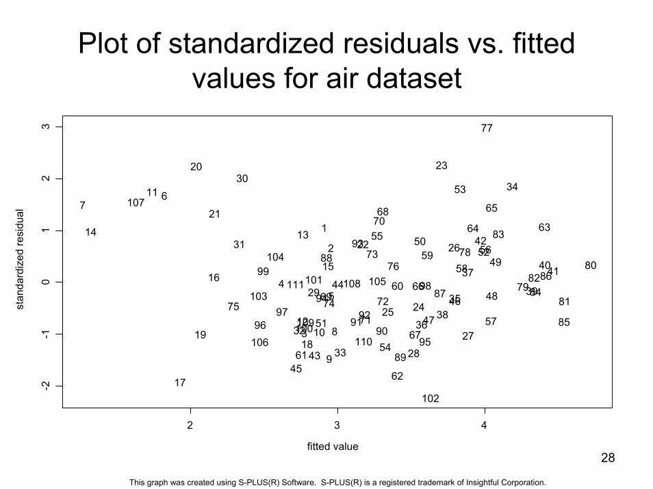
Plot of standardized residuals vs. fitted values for air dataset
fitted value
stan
dard
ized
resi
dual
2 3 4
-2-1
01
23
1
2
3
45
67
8
9
10
11
12
1314
1516
17
1819
20
21
22
23
2425
26
2728
29
30
31
32
33
34
35
36
37
38
39
4041
42
43
44
45
46
47
48
49
50
51
52
53
54
5556
57
5859
60
61
62
6364
65
66
67
68
69
70
71
72
73
7475
76
77
78
79
80
81
82
83
84
85
8687
88
89
909192
93
94
9596
97
9899
100
101
102
103
104
105
106
107
108
109
110
111
This graph was created using S-PLUS(R) Software. S-PLUS(R) is a registered trademark of Insightful Corporation.
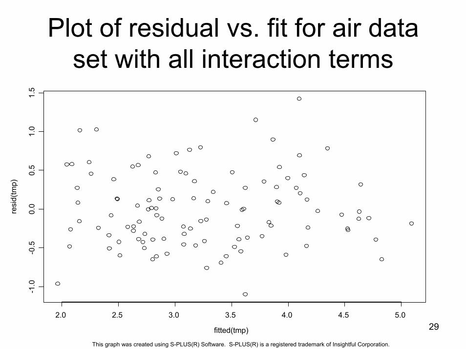
Plot of residual vs. fit for air data set with all interaction terms
fitted(tmp)
resi
d(tm
p)
2.0 2.5 3.0 3.5 4.0 4.5 5.0
-1.0
-0.5
0.0
0.5
1.0
1.5
This graph was created using S-PLUS(R) Software. S-PLUS(R) is a registered trademark of Insightful Corporation.
29
30
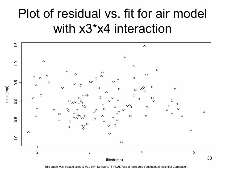
Plot of residual vs. fit for air model with x3*x4 interaction
fitted(tmp)
resi
d(tm
p)
2 3 4 5
-1.0
-0.5
0.0
0.5
1.0
1.5
This graph was created using S-PLUS(R) Software. S-PLUS(R) is a registered trademark of Insightful Corporation.
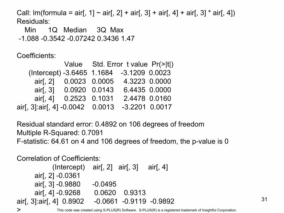
Call: lm(formula = air[, 1] ~ air[, 2] + air[, 3] + air[, 4] + air[, 3] * air[, 4])Residuals:
Min 1Q Median 3Q Max -1.088 -0.3542 -0.07242 0.3436 1.47
Coefficients:Value Std. Error t value Pr(>|t|)
(Intercept) -3.6465 1.1684 -3.1209 0.0023 air[, 2] 0.0023 0.0005 4.3223 0.0000 air[, 3] 0.0920 0.0143 6.4435 0.0000 air[, 4] 0.2523 0.1031 2.4478 0.0160
air[, 3]:air[, 4] -0.0042 0.0013 -3.2201 0.0017
Residual standard error: 0.4892 on 106 degrees of freedomMultiple R-Squared: 0.7091 F-statistic: 64.61 on 4 and 106 degrees of freedom, the p-value is 0
Correlation of Coefficients:(Intercept) air[, 2] air[, 3] air[, 4]
air[, 2] -0.0361 air[, 3] -0.9880 -0.0495 air[, 4] -0.9268 0.0620 0.9313
air[, 3]:air[, 4] 0.8902 -0.0661 -0.9119 -0.9892 >
31
This code was created using S-PLUS(R) Software. S-PLUS(R) is a registered trademark of Insightful Corporation.
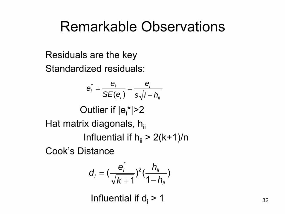
Remarkable Observations
Residuals are the keyStandardized residuals:
Outlier if |ei*|>2Hat matrix diagonals, hii
Influential if hii > 2(k+1)/nCook’s Distance
ii
i
i
ii his
eeSE
ee−
==)(
*
)1
()1
( 2*
ii
iiii h
hked
−+=
Influential if di > 1 32
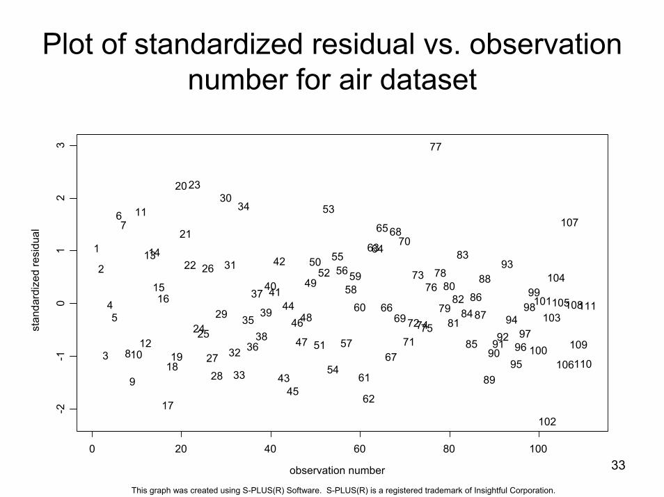
33
Plot of standardized residual vs. observation number for air dataset
observation number
stan
dard
ized
resi
dual
0 20 40 60 80 100
-2-1
01
23
1
2
3
45
67
8
9
10
11
12
1314
1516
17
1819
20
21
22
23
2425
26
2728
29
30
31
32
33
34
35
36
37
38
39
4041
42
43
44
45
46
47
48
49
50
51
52
53
54
5556
57
5859
60
61
62
6364
65
66
67
68
69
70
71
72
73
7475
76
77
78
79
80
81
82
83
84
85
8687
88
89
909192
93
94
959697
9899
100
101
102
103
104
105
106
107
108
109
110
111
This graph was created using S-PLUS(R) Software. S-PLUS(R) is a registered trademark of Insightful Corporation.
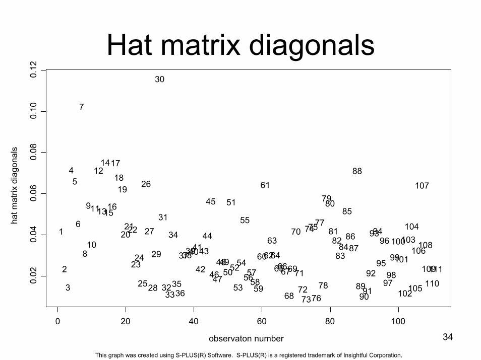
34
Hat matrix diagonals
observaton number
hat m
atrix
dia
gona
ls
0 20 40 60 80 100
0.02
0.04
0.06
0.08
0.10
0.12
1
2
3
45
6
7
8
9
10
11
12
13
14
1516
17
1819
202122
2324
25
26
27
28
29
30
31
3233
34
3536
3738394041
42
43
44
45
4647
484950
51
52
53
54
55
56575859
60
61
62
63
64656667
68
69
70
71
7273
7475
76
77
78
7980
8182
8384
85
8687
88
899091
92
9394
95
96
9798
99
100
101
102
103104
105
106
107
108
109
110111
This graph was created using S-PLUS(R) Software. S-PLUS(R) is a registered trademark of Insightful Corporation.
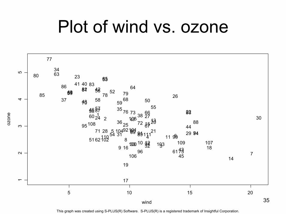
35
Plot of wind vs. ozone
wind
ozon
e
5 10 15 20
12
34
5
12
3
45
6
7
8
910
1112
13
14
15
16
17
18
19
20
21
22
23
2425
26
27
28 29
30
31
3233
34
35
36
37
38
39
404142
43
44
45
46
47
48
49
50
51
52
53
54
55
56
57
58 59
60
61
62
63
64
65
66
67
68
69
70
71
72
73
74
75
76
77
78 79
80
818283
8485
86
87
88
8990 91
92
93
9495
9697
98
99100
101
102103
104
105
106
107
108
109110 111
This graph was created using S-PLUS(R) Software. S-PLUS(R) is a registered trademark of Insightful Corporation.
36
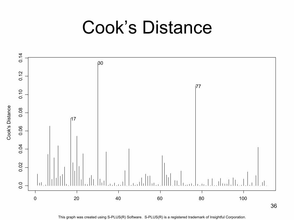
Cook’s DistanceC
ook'
s D
ista
nce
0 20 40 60 80 100
0.0
0.02
0.04
0.06
0.08
0.10
0.12
0.14
17
77
30
This graph was created using S-PLUS(R) Software. S-PLUS(R) is a registered trademark of Insightful Corporation.
37
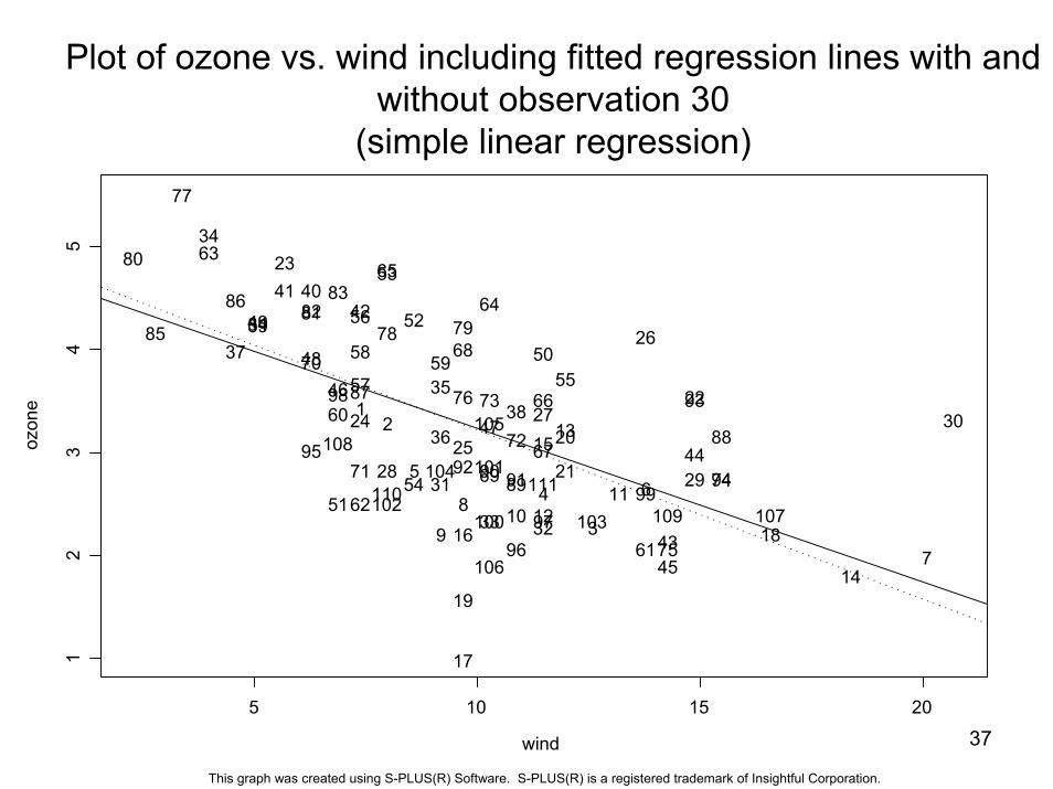
Plot of ozone vs. wind including fitted regression lines with and without observation 30
(simple linear regression)
wind
ozon
e
5 10 15 20
12
34
5
12
3
45
6
7
8
910
1112
13
14
15
16
17
18
19
20
21
22
23
2425
26
27
28 29
30
31
3233
34
35
36
37
38
39
404142
43
44
45
46
47
48
49
50
51
52
53
54
55
56
57
58 59
60
61
62
63
64
65
66
67
68
69
70
71
72
73
74
75
76
77
78 79
80
818283
8485
86
87
88
8990 91
92
93
9495
9697
98
99100
101
102103
104
105
106
107
108
109110 111
This graph was created using S-PLUS(R) Software. S-PLUS(R) is a registered trademark of Insightful Corporation.

Remedies for Outliers
• Nothing?• Data Transformation?• Remove outliers?• Robust Regression – weighted least
squares: b=(X’WX)-1X’Wy• Minimize median absolute deviation
38
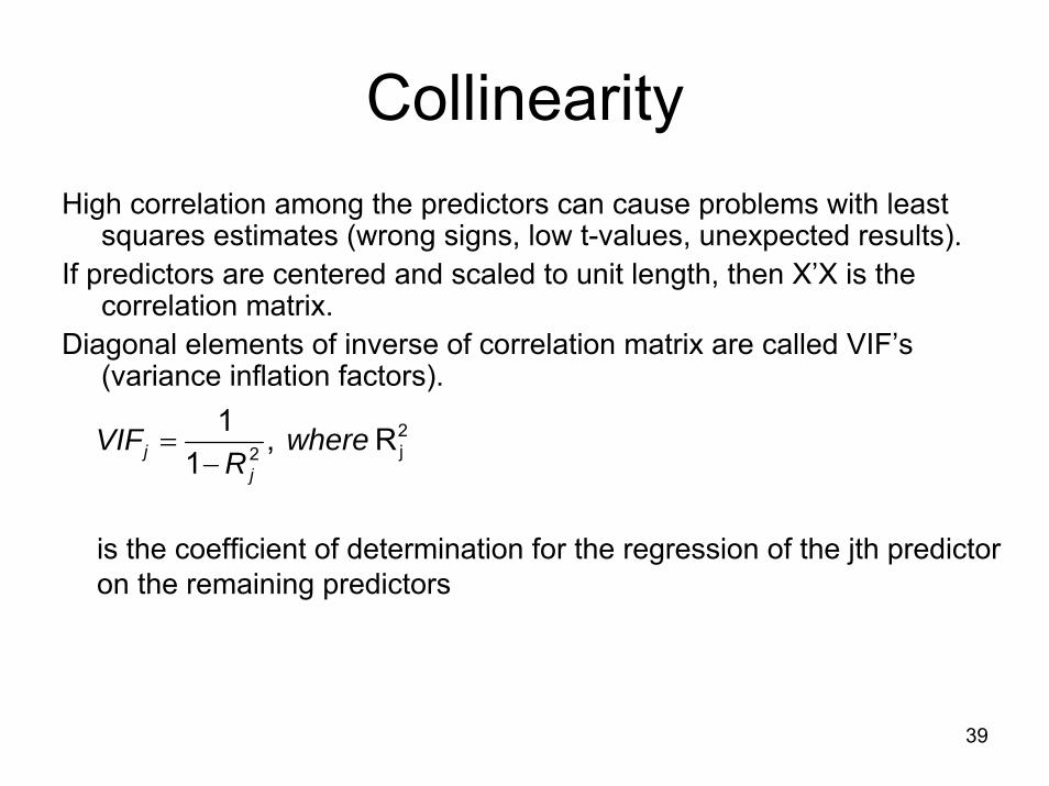
CollinearityHigh correlation among the predictors can cause problems with least
squares estimates (wrong signs, low t-values, unexpected results).If predictors are centered and scaled to unit length, then X’X is the
correlation matrix.Diagonal elements of inverse of correlation matrix are called VIF’s
(variance inflation factors).
R ,1
1 2j2 where
RVIF
jj −=
is the coefficient of determination for the regression of the jth predictor on the remaining predictors
39
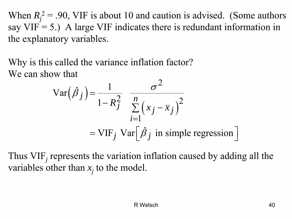
When Rj2 = .90, VIF is about 10 and caution is advised. (Some authors
say VIF = 5.) A large VIF indicates there is redundant information in the explanatory variables.
Why is this called the variance inflation factor?We can show that
Thus VIFj represents the variation inflation caused by adding all thevariables other than xj to the model.
( )( )
2
2 2
1
1ˆVar 1
ˆVIF Var in simple regression
j nj j j
i
j j
R x x
σβ
β=
=− −
⎡ ⎤= ⎣ ⎦
∑
R Welsch 40
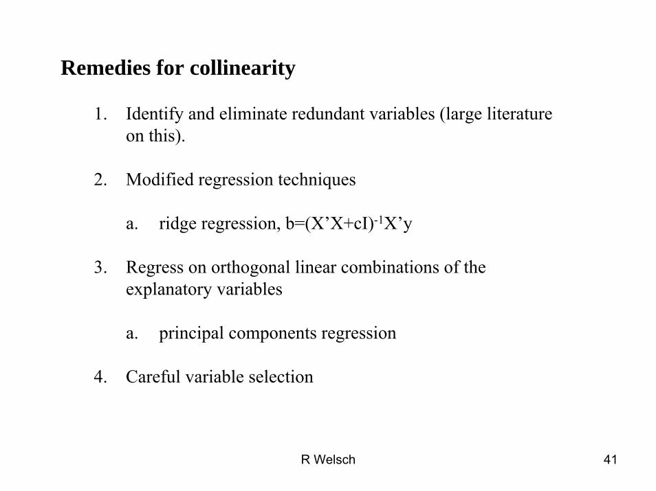
Remedies for collinearity
1. Identify and eliminate redundant variables (large literatureon this).
2. Modified regression techniques
a. ridge regression, b=(X’X+cI)-1X’y
3. Regress on orthogonal linear combinations of theexplanatory variables
a. principal components regression
4. Careful variable selection
R Welsch 41
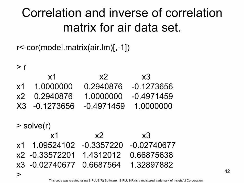
Correlation and inverse of correlation matrix for air data set.
r<-cor(model.matrix(air.lm)[,-1])
> rx1 x2 x3
x1 1.0000000 0.2940876 -0.1273656x2 0.2940876 1.0000000 -0.4971459X3 -0.1273656 -0.4971459 1.0000000
> solve(r)x1 x2 x3
x1 1.09524102 -0.3357220 -0.02740677x2 -0.33572201 1.4312012 0.66875638x3 -0.02740677 0.6687564 1.32897882 > 42
This code was created using S-PLUS(R) Software. S-PLUS(R) is a registered trademark of Insightful Corporation.
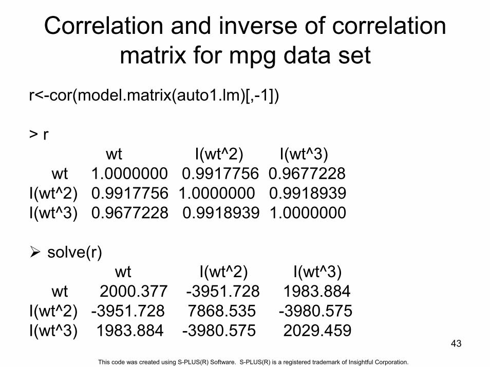
Correlation and inverse of correlation matrix for mpg data set
r<-cor(model.matrix(auto1.lm)[,-1])
> rwt I(wt^2) I(wt^3)
wt 1.0000000 0.9917756 0.9677228I(wt^2) 0.9917756 1.0000000 0.9918939I(wt^3) 0.9677228 0.9918939 1.0000000
solve(r)wt I(wt^2) I(wt^3)
wt 2000.377 -3951.728 1983.884I(wt^2) -3951.728 7868.535 -3980.575I(wt^3) 1983.884 -3980.575 2029.459
43
This code was created using S-PLUS(R) Software. S-PLUS(R) is a registered trademark of Insightful Corporation.
Variable Selection
• We want a parsimonious model – as few variables as possible to still provide reasonable accuracy in predicting y.
• Some variables may not contribute much to the model.
• SSE never will increase if add more variables to model, however MSE=SSE/(n-k-1) may.
• Minimum MSE is one possible optimality criterion. However, must fit all possible subsets (2k of them) and find one with minimum MSE.
44
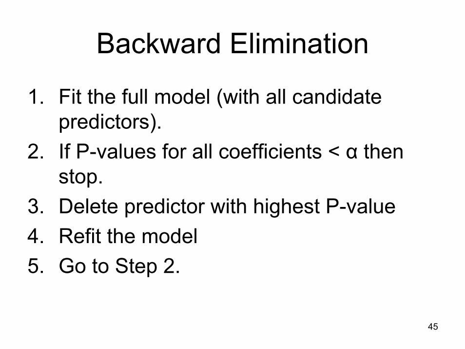
Backward Elimination
1. Fit the full model (with all candidate predictors).
2. If P-values for all coefficients < α then stop.
3. Delete predictor with highest P-value4. Refit the model5. Go to Step 2.
45