Muffin Tins, Green’s Functions, and Nanoscale Transport

[ ] 1−Σ−−= RR HEG

Derek StewartCNF Fall WorkshopCooking Lesson #1

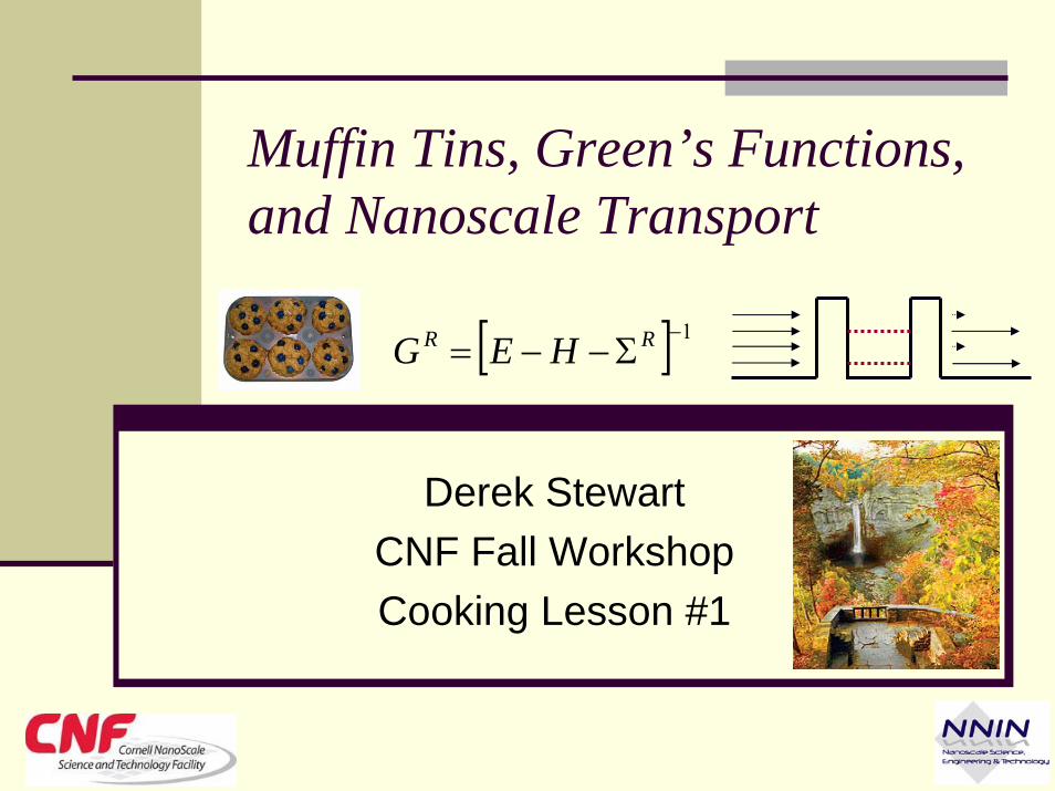
Talk Overview

A more localized approachOrigins: Multiple Scattering Theory & KKR

Linear Muffin Tin Orbitals

Green’s functions and TransportGreen’s Function basics

Tight binding models

Transport

[ ] 1−Σ−−= RR HEG

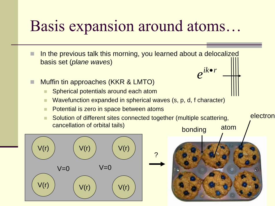
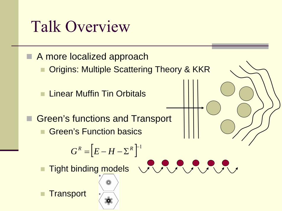
Basis expansion around atoms…In the previous talk this morning, you learned about a delocalized basis set (plane waves)

Muffin tin approaches (KKR & LMTO)Spherical potentials around each atomWavefunction expanded in spherical waves (s, p, d, f character)Potential is zero in space between atomsSolution of different sites connected together (multiple scattering, cancellation of orbital tails)

V(r) V(r)

V(r) V(r)

V(r)

V(r)

V=0 V=0

electron

?

rike •

atombonding

Multiple Scattering Theory (MST)From Point Scatterers to Solids

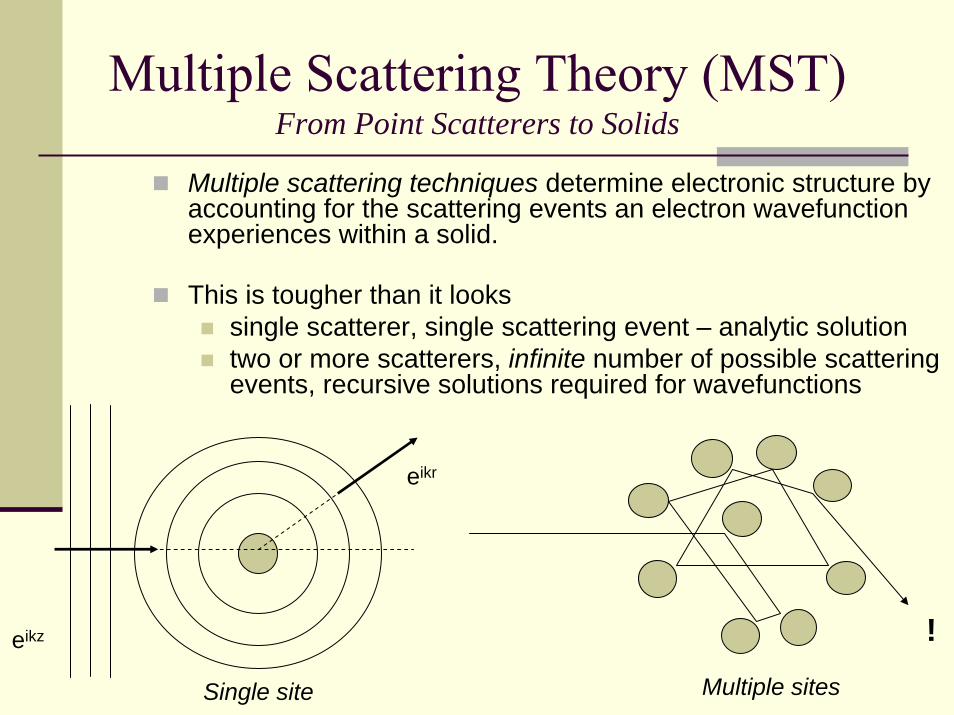
Multiple scattering techniques determine electronic structure by accounting for the scattering events an electron wavefunctionexperiences within a solid.

This is tougher than it lookssingle scatterer, single scattering event – analytic solutiontwo or more scatterers, infinite number of possible scattering events, recursive solutions required for wavefunctions

!

eikr

Multiple sites

eikz

Single site

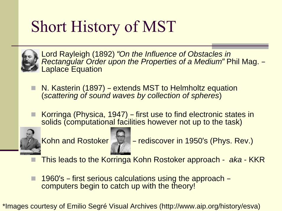
Short History of MSTLord Rayleigh (1892) “On the Influence of Obstacles in Rectangular Order upon the Properties of a Medium” Phil Mag. –Laplace Equation

N. Kasterin (1897) – extends MST to Helmholtz equation (scattering of sound waves by collection of spheres)

Korringa (Physica, 1947) – first use to find electronic states in solids (computational facilities however not up to the task)

Kohn and Rostoker – rediscover in 1950’s (Phys. Rev.)

This leads to the Korringa Kohn Rostoker approach - aka - KKR

1960’s – first serious calculations using the approach –computers begin to catch up with the theory!

*Images courtesy of Emilio Segré Visual Archives (http://www.aip.org/history/esva)

So your system has potential….

[ ] ( ) ( )rErVHorr ψψ =+

-Ho is the free space Hamiltonian-V is the perturbing potential−Ψ is the electron wavefunction

( ) ( ) ( ) ( ) ( ) rdrrrrGrr o ′′′′+= ∫ 3V, rrrrrr ψχψ

We can express the wavefunction at some position as a sum of thefree space wavefunction, χ, with no perturbing potential, and contributions from the perturbing potential, V, at different sites.

In this case, Go is the free electron propagator and describes motionin regions where no scattering from the potential occurs.

Letting Green do the expansion

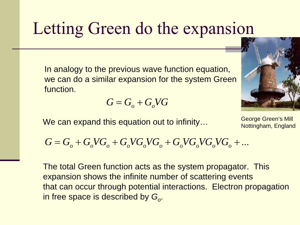
In analogy to the previous wave function equation, we can do a similar expansion for the system Green function.

VGGGG oo +=George Green’s MillNottingham, EnglandWe can expand this equation out to infinity…

...++++= oooooooooo VGVGVGGVGVGGVGGGG

The total Green function acts as the system propagator. Thisexpansion shows the infinite number of scattering events that can occur through potential interactions. Electron propagationin free space is described by Go.

Introducing the T matrix

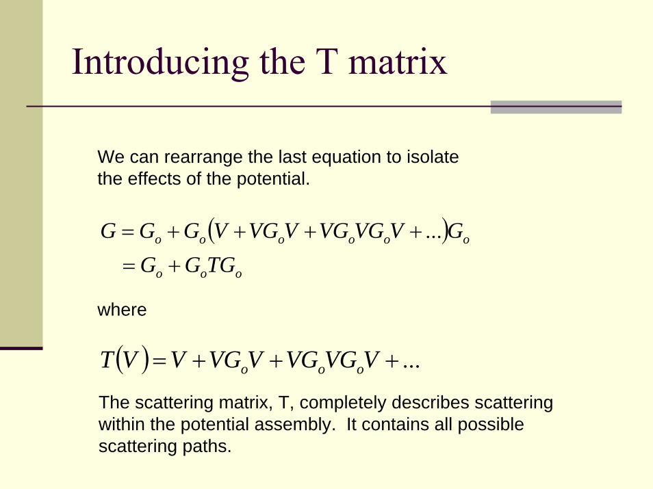
We can rearrange the last equation to isolate the effects of the potential.

( )ooo

oooooo

TGGGGVVGVGVVGVGGG

+=++++=

...

where

( ) ...+++= VVGVGVVGVVT ooo

The scattering matrix, T, completely describes scatteringwithin the potential assembly. It contains all possiblescattering paths.

Multiple Scattering Sites

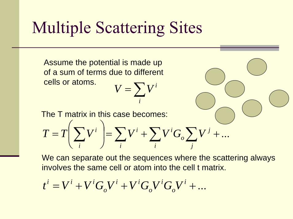
Assume the potential is made upof a sum of terms due to differentcells or atoms.

∑=i

iVV

The T matrix in this case becomes:

...++=⎟⎠

⎞⎜⎝

⎛= ∑∑∑∑

j

jo

i

i

i

i

i

i VGVVVTT

We can separate out the sequences where the scattering alwaysinvolves the same cell or atom into the cell t matrix.

...+++= io

io

iio

iii VGVGVVGVVt

Atomic t matrix uncovered

Solve the radial Schrodinger’s equation for an isolated muffin tin potential and determine the regular andirregular solutions, Z and S.

The atomic t matrix is diagonal in the angular momentumrepresentation.

lill eit δα δsin=

The phase shift, δ, can be found from the atomic wavefunction.

All the possible paths…

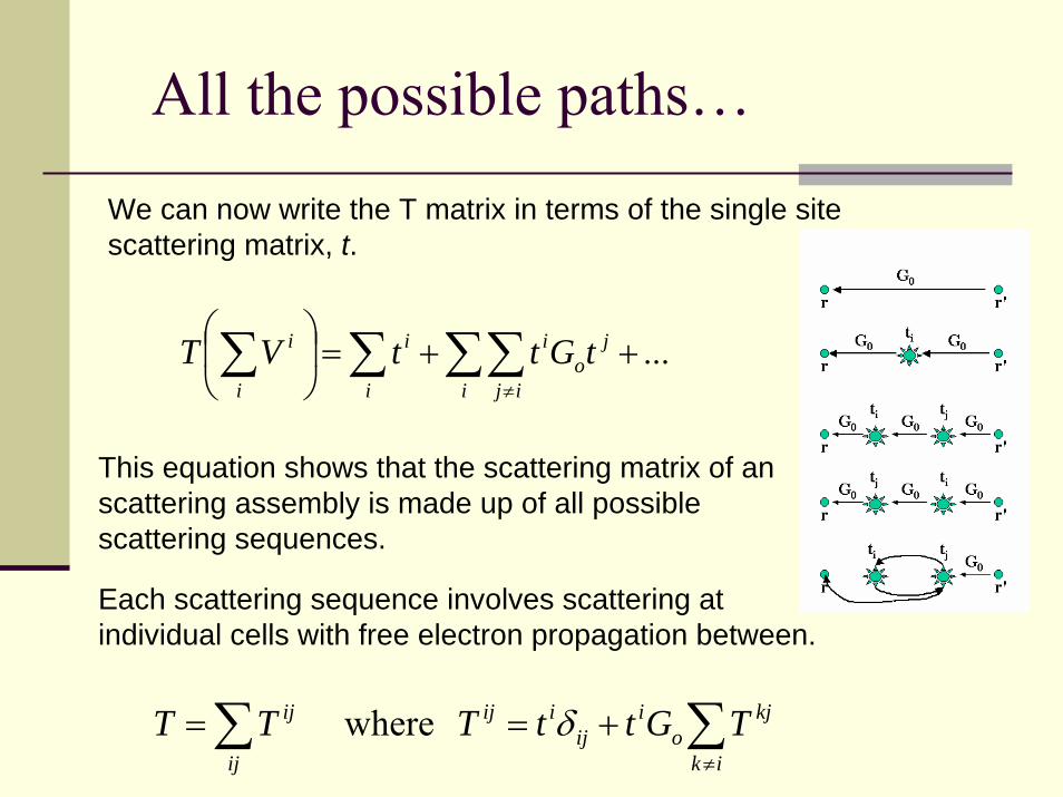
We can now write the T matrix in terms of the single sitescattering matrix, t.

...++=⎟⎠

⎞⎜⎝

⎛ ∑∑∑∑≠i ij

jo

i

i

i

i

i tGttVT

This equation shows that the scattering matrix of an scattering assembly is made up of all possible scattering sequences.

Each scattering sequence involves scattering at individual cells with free electron propagation between.

∑∑≠

+==ik

kjo

iij

iij

ij

ij TGttTTT δ where

Getting the Band Together

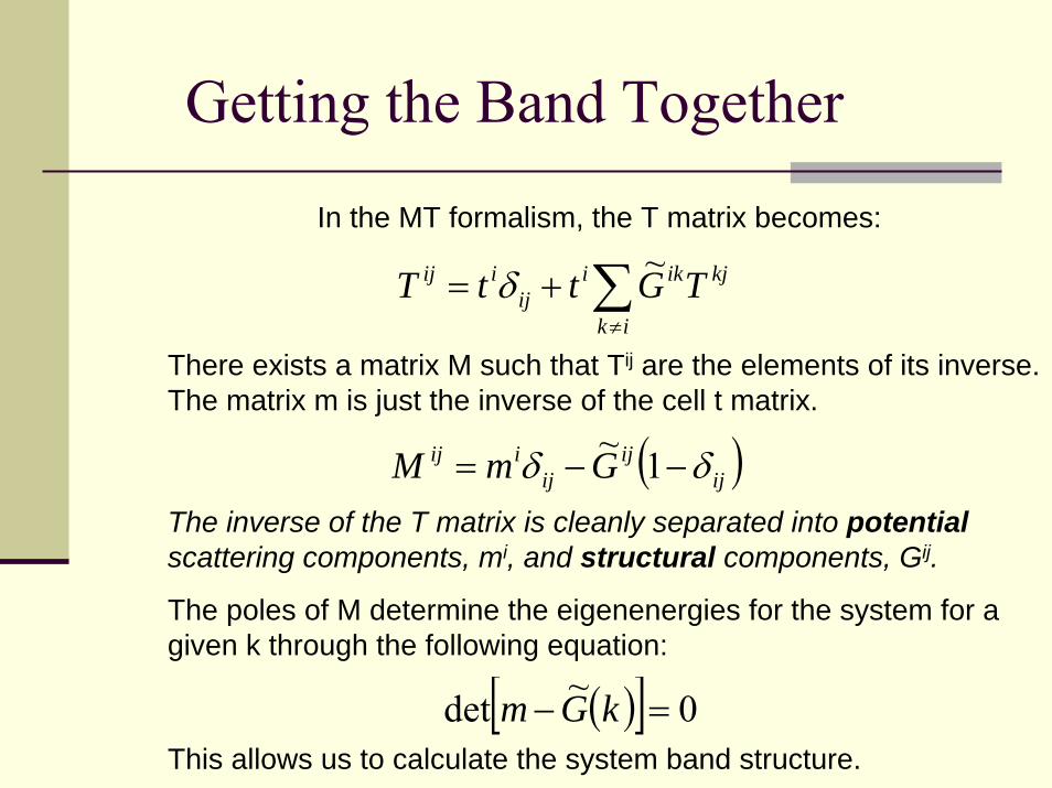
In the MT formalism, the T matrix becomes:

∑≠

+=ik

kjikiij

iij TGttT ~δ

There exists a matrix M such that Tij are the elements of its inverse.The matrix m is just the inverse of the cell t matrix.

( )ijij

ijiij GmM δδ −−= 1~

The inverse of the T matrix is cleanly separated into potentialscattering components, mi, and structural components, Gij.

The poles of M determine the eigenenergies for the system for a given k through the following equation:

( )[ ] 0~det =− kGmThis allows us to calculate the system band structure.

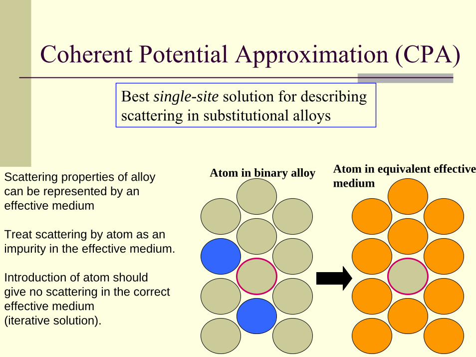
Coherent Potential Approximation (CPA)Best single-site solution for describing scattering in substitutional alloys

Scattering properties of alloycan be represented by an effective medium

Treat scattering by atom as animpurity in the effective medium.

Introduction of atom should give no scattering in the correcteffective medium (iterative solution).

Atom in binary alloy Atom in equivalent effectivemedium

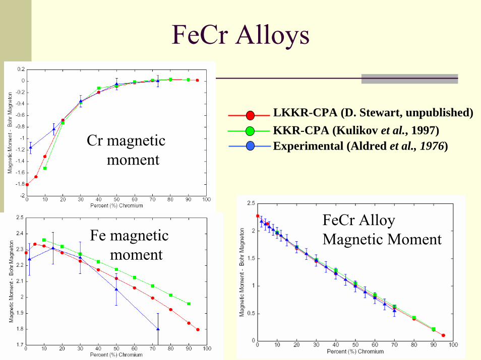
FeCr Alloys

Cr magnetic moment

Fe magnetic moment

LKKR-CPA (D. Stewart, unpublished)KKR-CPA (Kulikov et al., 1997)Experimental (Aldred et al., 1976)

FeCr Alloy Magnetic Moment

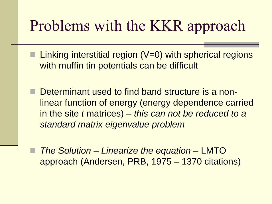
Problems with the KKR approach

Linking interstitial region (V=0) with spherical regions with muffin tin potentials can be difficult

Determinant used to find band structure is a non-linear function of energy (energy dependence carried in the site t matrices) – this can not be reduced to a standard matrix eigenvalue problem

The Solution – Linearize the equation – LMTO approach (Andersen, PRB, 1975 – 1370 citations)

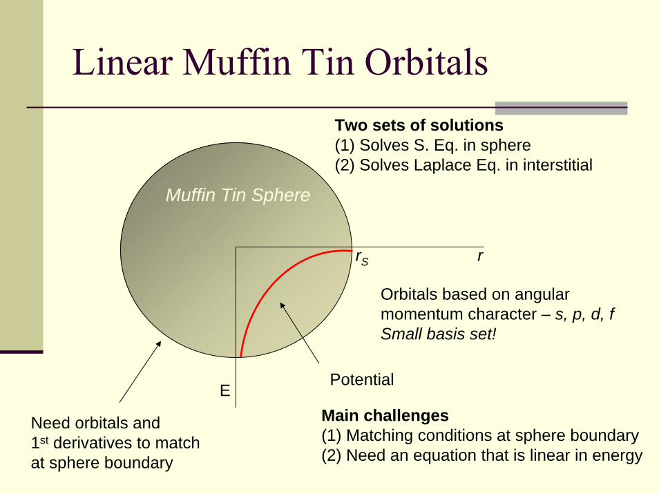
Linear Muffin Tin Orbitals

Muffin Tin Sphere

r

Potential

Two sets of solutions(1) Solves S. Eq. in sphere(2) Solves Laplace Eq. in interstitial

E

rS

Orbitals based on angular momentum character – s, p, d, fSmall basis set!

Main challenges(1) Matching conditions at sphere boundary(2) Need an equation that is linear in energy

Need orbitals and 1st derivatives to match at sphere boundary

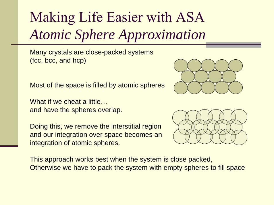
Making Life Easier with ASAAtomic Sphere ApproximationMany crystals are close-packed systems (fcc, bcc, and hcp)

Most of the space is filled by atomic spheres

What if we cheat a little…and have the spheres overlap.

Doing this, we remove the interstitial regionand our integration over space becomes anintegration of atomic spheres.

This approach works best when the system is close packed,Otherwise we have to pack the system with empty spheres to fill space

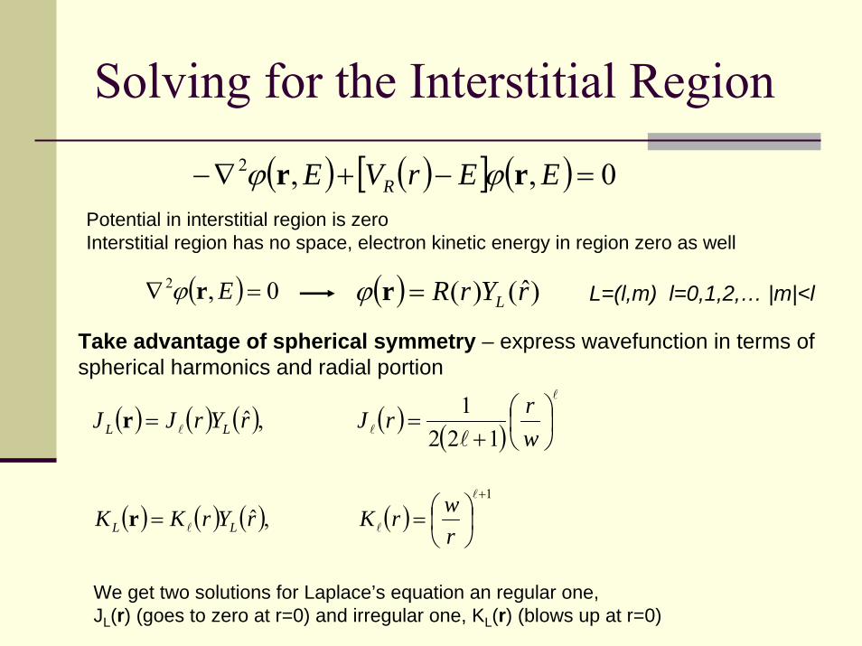
Solving for the Interstitial Region

( ) ( )[ ] ( ) 0,,2 =−+∇− EErVE R rr ϕϕPotential in interstitial region is zeroInterstitial region has no space, electron kinetic energy in region zero as well

( ) )ˆ()( rYrR L=rϕ( ) 0,2 =∇ Erϕ L=(l,m) l=0,1,2,… |m|<l

( ) ( ) ( ) ( ) ( )l

lll

⎟⎠⎞

⎜⎝⎛

+==

wrrJrYrJJ LL 122

1 ,ˆr

Take advantage of spherical symmetry – express wavefunction in terms of spherical harmonics and radial portion

( ) ( ) ( ) ( )1

,ˆ+

⎟⎠⎞

⎜⎝⎛==

l

ll rwrKrYrKK LL r

We get two solutions for Laplace’s equation an regular one, JL(r) (goes to zero at r=0) and irregular one, KL(r) (blows up at r=0)

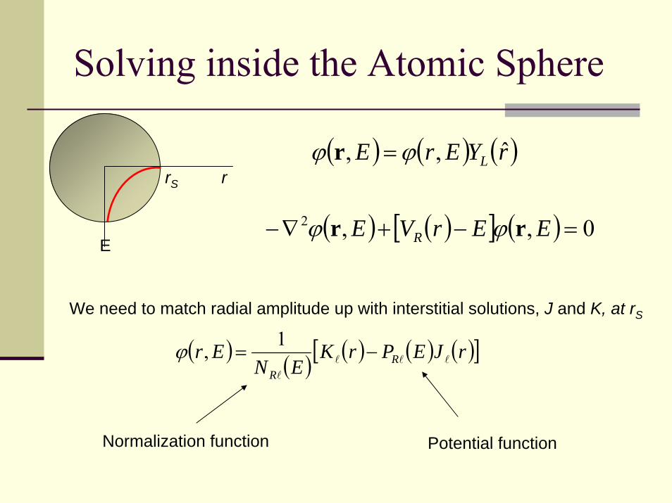
Solving inside the Atomic Sphere

r

E

rS

( ) ( ) ( )rYErE L ˆ,, ϕϕ =r

( ) ( )[ ] ( ) 0,,2 =−+∇− EErVE R rr ϕϕ

We need to match radial amplitude up with interstitial solutions, J and K, at rS

( ) ( ) ( ) ( ) ( )[ ]rJEPrKEN

Er RR

lll

l

−=1,ϕ

Normalization function Potential function

Muffin Tin Orbitals

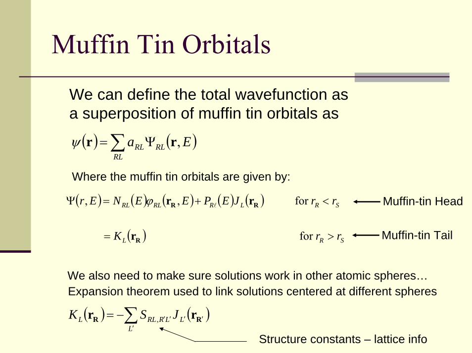
We can define the total wavefunction as a superposition of muffin tin orbitals as

( ) ( )∑ Ψ=RL

RLRL Ea ,rrψ

Where the muffin tin orbitals are given by:

( ) ( ) ( ) ( ) ( )

( ) SRL

SRLRRLRL

rrK

rrJEPEENEr

>=

<+=Ψ

for

for ,,

R

RR

r

rr lϕ Muffin-tin Head

Muffin-tin Tail

We also need to make sure solutions work in other atomic spheres…Expansion theorem used to link solutions centered at different spheres

( ) ( )∑′

′′′′−=L

LLRRLL JSK RR rr ,

Structure constants – lattice info

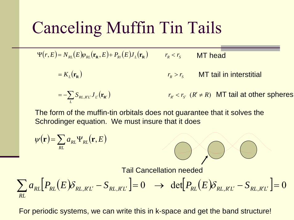
Canceling Muffin Tin Tails( ) ( ) ( ) ( ) ( )

( )

( ) )(

,,

, RRrrJS

rrK

rrJEPEENEr

SRL

LLRRL

SRL

SRLRRLRL

≠′<−=

>=

<+=Ψ

′′′′′′∑ R

R

RR

r

r

rr lϕ MT head

MT tail in interstitial

MT tail at other spheres

The form of the muffin-tin orbitals does not guarantee that it solves theSchrodinger equation. We must insure that it does

( ) ( )∑ Ψ=RL

RLRL Ea ,rrψ

Tail Cancellation needed

( )[ ] ( )[ ] 0det 0 ,,,, =−→=−∑ ′′′′′′′′RL

LRRLLRRLRLLRRLLRRLRLRL SEPSEPa δδ

For periodic systems, we can write this in k-space and get the band structure!

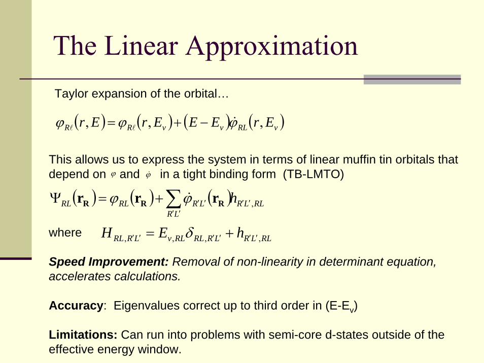
The Linear ApproximationTaylor expansion of the orbital…

( ) ( ) ( ) ( )vRLvvRR ErEEErEr ,,, ϕϕϕ &ll −+=

This allows us to express the system in terms of linear muffin tin orbitals thatdepend on and in a tight binding form (TB-LMTO)

where

Speed Improvement: Removal of non-linearity in determinant equation, accelerates calculations.

Accuracy: Eigenvalues correct up to third order in (E-Ev)

Limitations: Can run into problems with semi-core d-states outside of the effective energy window.

ϕ&ϕ

( ) ( ) ( ) RLLRLR

LRRLRL h ,′′′′

′′∑+=Ψ RRR rrr ϕϕ &

RLLRLRRLRLvLRRL hEH ,,,, ′′′′′′ += δ

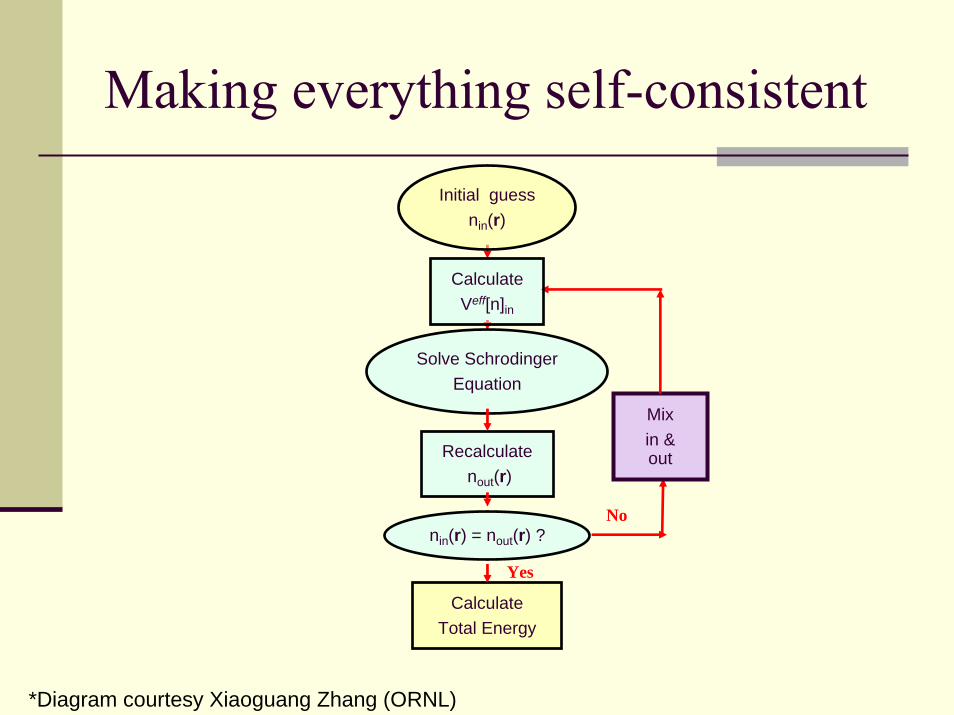
Making everything self-consistent

No

Yes

Mixin & out

Initial guessnin(r)

CalculateVeff[n]in

Solve SchrodingerEquation

Recalculatenout(r)

nin(r) = nout(r) ?

CalculateTotal Energy

*Diagram courtesy Xiaoguang Zhang (ORNL)

Coming up this afternoon

LMTO commandsRunning LMTO calculations

Silicon – role of empty spheresMagnetic properties – NickelDensity of states, band structure, etc

An Introduction to Green’s Functions

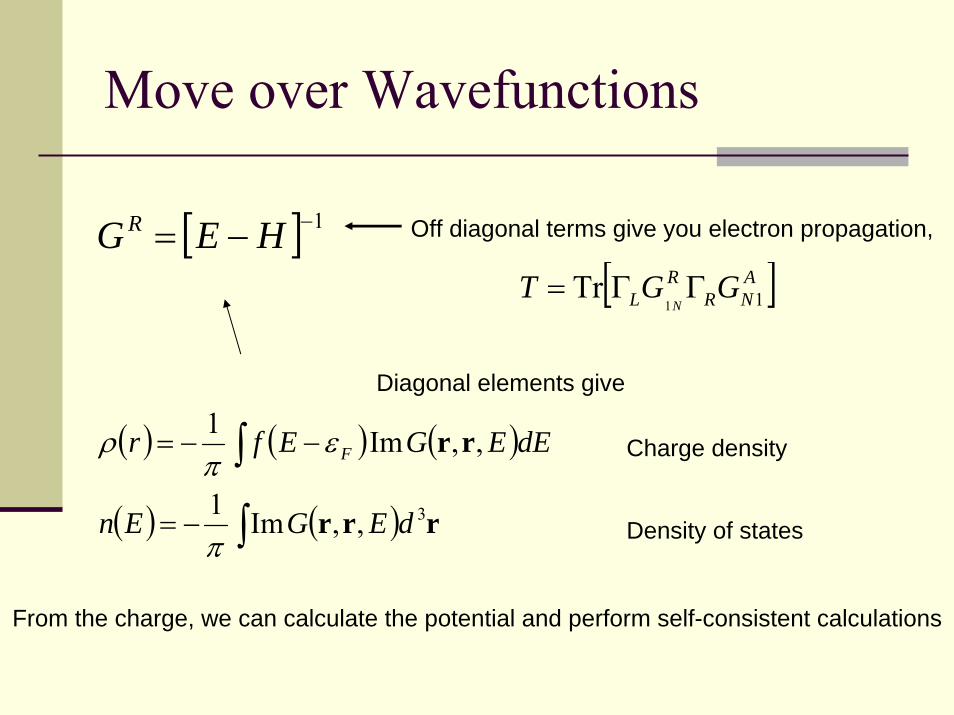
Move over Wavefunctions

[ ] 1−−= HEGR Off diagonal terms give you electron propagation,

[ ]ANR

RL GGT

N 11Tr ΓΓ=

Diagonal elements give

( ) ( ) ( )

( ) ( )∫

∫

−=

−−=

rrr

rr

3,,Im1

,,Im1

dEGEn

dEEGEfr F

π

επ

ρ Charge density

Density of states

From the charge, we can calculate the potential and perform self-consistent calculations

Integration in the Complex Plane

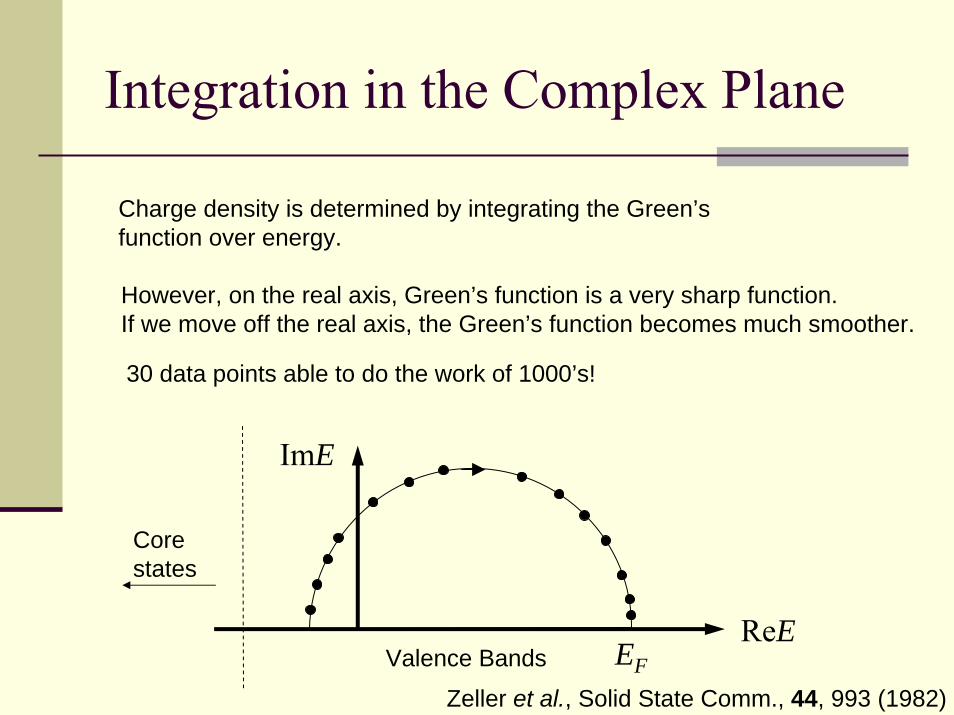
Charge density is determined by integrating the Green’sfunction over energy.

However, on the real axis, Green’s function is a very sharp function.If we move off the real axis, the Green’s function becomes much smoother.

30 data points able to do the work of 1000’s!

ReE

ImE

EF

Corestates

Valence Bands

Zeller et al., Solid State Comm., 44, 993 (1982)

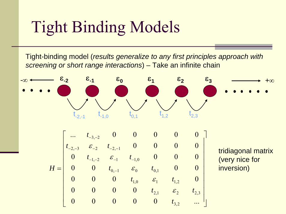
Tight Binding ModelsTight-binding model (results generalize to any first principles approach withscreening or short range interactions) – Take an infinite chain

ε-2 ε-1 ε0 ε1 ε2 ε3-∞ +∞

t-2,-1 t-1,0 t0,1 t1,2 t2,3

⎥⎥⎥⎥⎥⎥⎥⎥⎥

⎦

⎤

⎢⎢⎢⎢⎢⎢⎢⎢⎢

⎣

⎡

= −

−−−−

−−−−−

−−

...000000000

000000000000000000000...

2,3

3,221,2

2,110,1

1,001,0

0,112,1

1,223,2

2,3

ttt

tttt

tttt

t

H

εε

εε

εtridiagonal matrix (very nice for inversion)

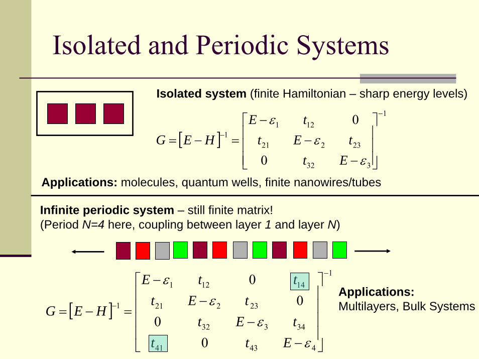
Isolated and Periodic SystemsIsolated system (finite Hamiltonian – sharp energy levels)

[ ]

1

332

23221

1211

0

0 −

−

⎥⎥⎥

⎦

⎤

⎢⎢⎢

⎣

⎡

−−

−=−=

εε

ε

EttEt

tEHEG

Applications: molecules, quantum wells, finite nanowires/tubes

Infinite periodic system – still finite matrix! (Period N=4 here, coupling between layer 1 and layer N)

[ ]

1

44341

34332

23221

14121

1

00

00 −

−

⎥⎥⎥⎥

⎦

⎤

⎢⎢⎢⎢

⎣

⎡

−−

−−

=−=

εε

εε

EtttEt

tEtttE

HEGApplications:Multilayers, Bulk Systems

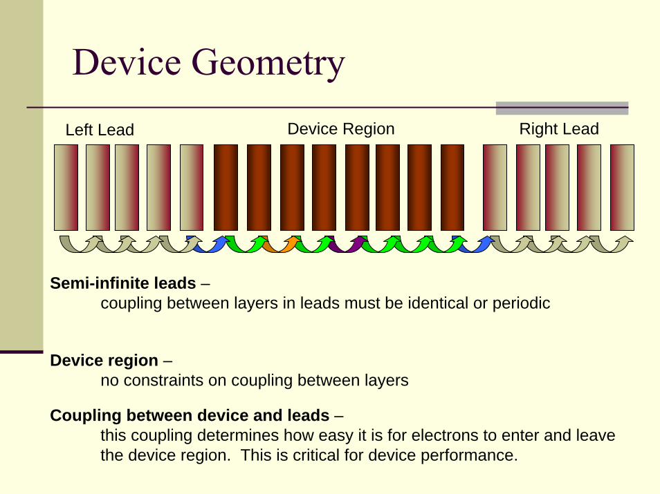
Device GeometryDevice Region Right LeadLeft Lead

Semi-infinite leads –coupling between layers in leads must be identical or periodic

Device region –no constraints on coupling between layers

Coupling between device and leads –this coupling determines how easy it is for electrons to enter and leavethe device region. This is critical for device performance.

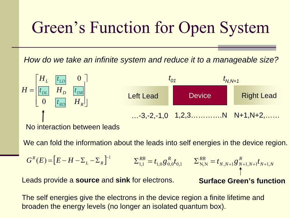
Green’s Function for Open System

How do we take an infinite system and reduce it to a manageable size?

[ ] 1)( −Σ−Σ−−= RLR HEEG

Device Right LeadLeft Lead⎥⎥⎥

⎦

⎤

⎢⎢⎢

⎣

⎡=

RRD

DRDDL

LDL

HttHt

tHH

0

0

No interaction between leads

t01 tN,N+1

1,2,3………….N N+1,N+2,………-3,-2,-1,0

We can fold the information about the leads into self energies in the device region.

NNR

NNNNRBRRB tgttgt ,11,11,NN,1,00,00,11,1 ++++=Σ=Σ

Leads provide a source and sink for electrons.

The self energies give the electrons in the device region a finite lifetime andbroaden the energy levels (no longer an isolated quantum box).

Surface Green’s function

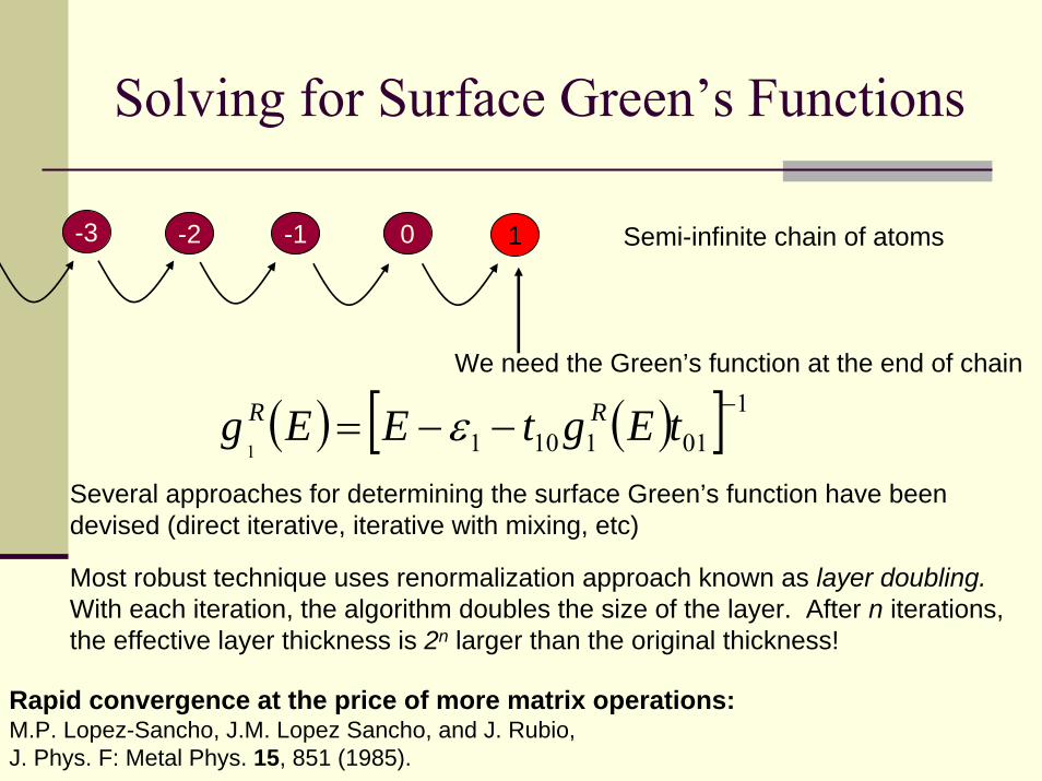
Solving for Surface Green’s Functions

-3 -2 -1 0 1 Semi-infinite chain of atoms

We need the Green’s function at the end of chain

( ) ( )[ ] 10111011

−−−= tEgtEEg RR ε

Several approaches for determining the surface Green’s function have beendevised (direct iterative, iterative with mixing, etc)

Most robust technique uses renormalization approach known as layer doubling. With each iteration, the algorithm doubles the size of the layer. After n iterations, the effective layer thickness is 2n larger than the original thickness!

Rapid convergence at the price of more matrix operations:M.P. Lopez-Sancho, J.M. Lopez Sancho, and J. Rubio, J. Phys. F: Metal Phys. 15, 851 (1985).

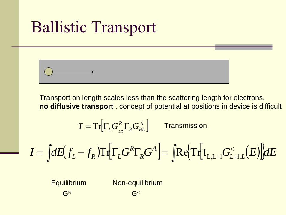
Ballistic Transport

Transport on length scales less than the scattering length for electrons,no diffusive transport , concept of potential at positions in device is difficult

[ ]ARLR

RL GGT

LRΓΓ= Tr Transmission

( ) [ ] ( )[ ] dEEGGGffdEI LLA

RR

LRL ∫∫ <++=ΓΓ−= ,11LL,tTrReTr

Equilibrium Non-equilibriumGR G<

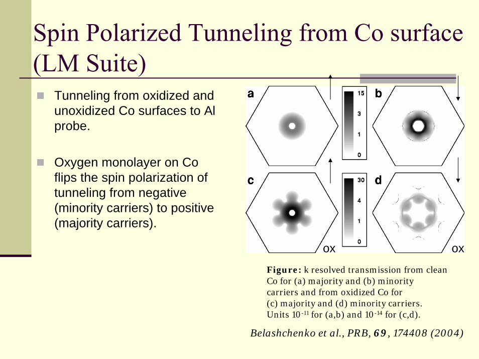
Spin Polarized Tunneling from Co surface (LM Suite)

Tunneling from oxidized and unoxidized Co surfaces to Al probe.

Oxygen monolayer on Co flips the spin polarization of tunneling from negative (minority carriers) to positive (majority carriers).

oxox

Figure: k resolved transmission from clean Co for (a) majority and (b) minoritycarriers and from oxidized Co for (c) majority and (d) minority carriers.Units 10-11 for (a,b) and 10-14 for (c,d).

Belashchenko et al., PRB, 69, 174408 (2004)

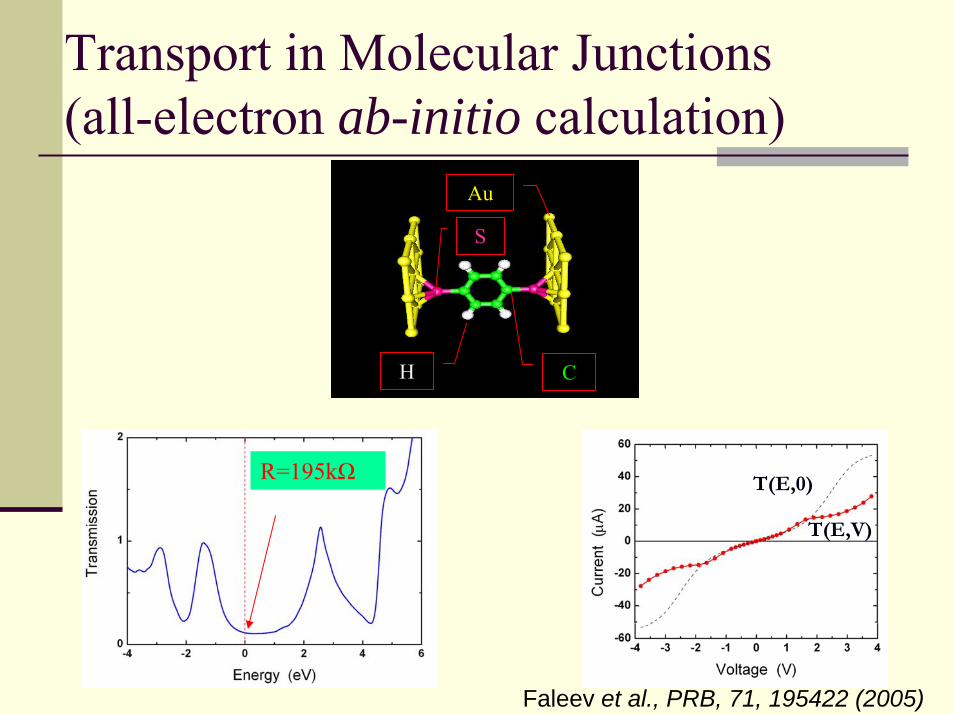
Transport in Molecular Junctions(all-electron ab-initio calculation)

H

Au

S

C

R=195kΩ

T(E,V)

T(E,0)

Faleev et al., PRB, 71, 195422 (2005)

Benefits of Green’s Function Approach

Capable of Handling Open Systems (something periodic DFT codes have trouble with)

System Properties (electronic charge, density of states, etc) without using wavefunctions

Ability to Handle Different Scattering Mechanisms through Self Energy Terms (not discussed here)

Natural Formalism for Transport Calculations