Estimating the International Transport Cost...

The International Gains fromDeclining Transport Costs

Ahmad Lashkaripour

Indiana University

October 2017

Abstract

This paper examines the welfare gains from transport cost re-

duction across six major economies. As a key step, I use detailed

firm-level trade data to estimate the transport cost elasticity, β, (i.e.,

the elasticity at which the unit transport cost varies with unit price)

for a wide range of industries. I estimate that (i) the transport

cost elasticity varies greatly across industries, and (ii) exhibits a

value of β = 0.8 for the average industry, which contrasts with the

widely-assumed but somewhat arbitrary unit elasticity specification.

Under the estimated elasticities, the gains from a 10% increase in

transportation efficiency are 2.34% for the average economy. In com-

parison, assuming a uniform and unit transport cost elasticity for all

industries understates the gains from transport cost reduction by

around 25%.

1 Introduction

The mass reduction in international transport costs is one the most strik-ing economic developments of last few decades. Driven by factors suchas containerization, this mass reduction has not only boosted the share oftrade in world GDP, but it has transformed the anatomy of global trade.Perhaps expectedly, this mass development has attracted the attention

1

of economists and policy-makers alike, with a multitude of quantita-tive models being developed to quantify the welfare consequences ofdeclining transport costs.

From the perspective of a state-of-the-art quantitative trade model, thegains from a reduction in transport costs are governed by two reduced-from elasticities: (i) the trade elasticity, which reflects the rate at whichtrade values decline with transport costs, and (ii) the transport costelasticity, β, which is the rate at which unit transport costs rise withthe unit price of traded goods. Of the two elasticities, the literature hasdevoted considerable attention to estimating and incorporating the roleof the trade elasticity. But the transport cost elasticity is often arbitrarilynormalized to one (i.e., β = 1), leading to the well-known multiplicativeor iceberg transport cost specification.

The widespread normalization of the transport cost elasticity is moti-vated by two considerations. First, under β = 1, the welfare gains fromtransport cost reduction can be calculated based solely on macro-levelimport shares—see Arkolakis et al. (2012); Costinot and Rodríguez-Clare(2013), as well as Donaldson (2018) for an empirical application. To bemore specific, the iceberg specification implied by β = 1, entails that anacross-the-board reduction in transport costs does not distort relativeprices across firms. Hence, one can quantify the resulting welfare effectsbased solely on macro-level import shares, without explicit knowledgeabout micro-level price heterogeneity. Correspondingly, relaxing β = 1,the gains from transport cost reduction depend not only on macro-levelimport shares but also on the entire schedule of firm-level prices.

The second consideration is that we know surprisingly little about theempirical magnitude of the transport cost elasticity. Many studies havechallenged the iceberg specification arising from β = 1;1 but less attentionhas been paid to the actual estimation of β itself. A notable exception isHummels and Skiba (2004), who estimate the economy-wide transportcost elasticity to test the celebrated Alchain-Allen hypothesis.

The aggregate and scant nature of the data employed by Hummels and

1See for example Irarrazabal et al. (2014), Sørensen (2014), and Martin (2012).

2

Skiba (2004), however, exposed them to two basic challenges. First, tomeasure unit prices and transport costs, they had to infer import quanti-ties from data on physical weight. As a result, they estimate β conditionalon the identifying assumption that unit weight is uniform within productcategories. Second, they had to deal with simultaneity between unitprices and transport costs, which is increasingly difficult when dealingwith highly-aggregated data. Perhaps due to these limitations, the esti-mates of Hummels and Skiba (2004) were never fully implemented intosubsequent analyses of global transport cost reduction.

Considering the above background, to credibly quantify the gains fromtransport cost reduction, I employs rich transaction-level trade data toestimate the transport cost elasticity for a wide range of industries. As anintermediate step, I show that the identifying assumption in Hummelsand Skiba (2004) regarding the uniformity of import unit weights isempirically violated. That is, import unit weights vary widely even withinnarrowly-defined categories, and theses variations are systematic: (i)import unit weights increase systematically with unit prices (i.e., valuablemerchandise are heavier), (ii) heavy merchandise are sourced relativelymore from rich countries and relatively less from distant suppliers, and(iii) imported merchandise are becoming lighter over time. Importantly,not accounting for these systematic variations can lead to an omittedvariable bias that attenuates β.

To deal with the simultaneity problem underlying the estimation of β,I employ two strategies that capitalize on the detailed nature of thedata. First, I identify β while conditioning on firm-product-year fixedeffects. Second, I utilize transaction-level information on the identityof exporting firms and importing entities. This information allows meto instrument for shipment-level prices, with the average price paidby an importing entity on alternative routes for goods purchased fromalternative suppliers. This instrument is a remarkably strong predictorof import price levels, and is conceivably orthogonal to route-specificmovements in transportation costs.

Overall, my estimation results suggest that the transport cost elasticityvaries considerably across industries. The estimated transport cost elas-

3

ticity is lowest in the Food and Beverage industries, where it averagesround β = 0.3, and highest in Transportation Equipment and Machinery,where it averages around β = 1. For the average industry I estimate thatβ = 0.8, which rejects the iceberg specification but not as extremely astraditional estimates. Aside from utilizing more detailed data, my higher-than-traditional estimate for β is primarily a consequence of accountingfor the systematic variation in import unit weights.2

In the second stage of my analysis, I plug the micro-estimated transportcost elasticities into a structural model to quantify the gains from trans-port cost reduction for six major economies: Brazil, China, the EuropeanUnion, India, Japan, and the United States. My analysis here involves cal-ibrating a multi-country trade model to match industry-level productionand trade data across 7 regions and 33 industries.

Using the calibrated model, I calculate that (on average) a 10% increasein transportation efficiency leads to 2.34% increase in real per capitaincome with respect to the manufacturing and agricultural sectors. Incomparison, assuming a uniform and unit transport cost elasticity (β = 1),which is standard in the literature, reduces the calculated gains by 25%.There is a simple intuition behind this finding. When β < 1, transportcosts distort the distribution of relative consumer prices. The dominantapproach in the literature neglects this distortion. However, in practice,by mitigating this distortion, transport cost reductions can lead to greater-than-perviously-estimated welfare gains.

The above results contribute to a vibrant empirical literature on the gainsfrom inter- or intra-national transport cost reduction (e.g., Donaldson(2018); Donaldson and Hornbeck (2016); Atkin and Donaldson (2015)).As note earlier, the dominant approach in the literature is to calculatewelfare gains conditional on the unit transport cost elasticity specification,

2There is a simple intuition for why overlooking the variation in import unit weightsattenuates the estimated transport cost elasticity. High-price items are costlier to trans-port due to (i) being heavier and (ii) the greater insurance, packaging and handlingrequirements associated with high-value merchandise. By treating unit weight as uni-form, traditional estimates overlook the former channel, and understate the elasticityof transport cost with respect to unit price. Accounting for both channels, however,transport costs increase near proportionally with unit price, thereby resembling icebergmelt costs.

4

i.e., β = 1. The results presented in this paper suggest that this approachmay systematically understate the corresponding welfare gains.

The present paper is also closely related to a literature that studies thedeterminants of international transport costs (Hummels and Skiba (2004);Clark et al. (2004); Hummels et al. (2009); Blonigen and Wilson (2008); Abeand Wilson (2009)). My contribution to this literature is two-fold. First,this paper is the first to explicitly account for the role of physical weightin international transportation. Second, whereas previous studies havefocused on country-level trade data, I shed new light on the anatomy ofinternational transportation using detailed transaction-level data. Giventhe focus of the paper and in-line with Hummels and Skiba (2004), Iemploy the direct approach of estimating the transport cost elasticityusing data on freight plus insurance rates. Nonetheless, my estimationresults are consistent with those in Irarrazabal et al. (2014), who use anindirect approach to infer the underlying structure of international tradebarriers, which are broadly-defined and includes tariffs, transport cost,and non-tangible red tape barriers among other things.

At a broader level, this paper sheds new light on an ongoing debate aboutthe consequences of micro-level heterogeneity for the welfare gains fromtrade. On one hand, Arkolakis et al. (2012) argue that the incorporation ofmicro-level heterogeneity may be of no consequence for the macro-levelgains from trade. On the other hand, several studies including Melitzand Redding (2015) and Simonovska and Waugh (2014) have challengedthis assertion. From a theoretical point, this paper demonstrates thatmicro-level price heterogeneity is consequential for macro-level welfaregains, except in the knife-edge case were β = 1. Empirically, I show thatwhile this knife-edge assumption holds in certain industries, it is violatedin many others.

Finally, this paper provides a glimpse into an unexplored avenue thatwarrants further research. While often neglected in the literature, I findthat physical weight plays a dominant role in international transportation,and that its role has been evolving rapidly over time. A better under-standing of global trade conceivably requires a better understanding ofthese developments.

5

2 Theoretical Framework

I first present a basic theory that highlights the welfare gains from trans-port cost reduction. To this end, I use a generic trade model that nests animportant class of workhorse quantitative trade models as a special case.This level of generality will allow me to put the dominant approach inthe literature in perspective and to outline its underlying limitations.

Economic Environment and Preferences. The global economy consistsare N countries indexed by j and i, plus K industries index by k. Theutility of the representative consumer in country i can be stated as

Wi = Ui (Qi,1, ..., Qi,K) ,

where Qi,k is a utility aggregator across all firm varieties from variouscountries of origin in industry k. More specifically, Qi,k = Qi,k(qωi,k),where qωi,k denotes the quantity purchased from firm ω in industry k.

Production and Transportation. On the production side, country i ispopulated with Li units of a Hicksian composite factor of production,which is employed in either final good production or transportation. wi

denotes the factor price in country i. Each country is also populatedwith a mass of perfectly competitive firms, indexed by ω. The total costfacing firm ω from industry k in country i is cω,k = cω,k(q; wi), which isincreasing in total output q.

Firm ω collects a factory-gate (f.o.b.) price, pω,k, for its output that isequal to marginal cost. The consumer (c.i.f. ) price for firm ω’s outputin market i, πωi,k, is the sum of the f.o.b. price plus a transportation cost,τωi,k. In particular,

πji,k = pω,k + τωi,k.

The transportation cost, τωi,k is composed of (i) an aggregate cost-shifterthat accounts for factors such as aggregate transportation efficiency, geo-distance, and administrative barriers, plus (ii) a firm-specific term thataccounts for the fact that freight companies charge rates based on the

6

value of transported items. Formally stated,3

τωi,k = tji,k · fk(pω,k, wi),

where fk(., .) is increasing in both arguments. Note that the dependenceof τωi,k on pωi,k accounts for, among other things, scale effects in trans-portation. Specifically, the variation in f.o.b. price affects total salesand therefore shipment scale, which can ultimately alter the unit cost oftransportation.

Following Hummels and Skiba (2004), I hereafter define βk ≡∂ ln τωi,k∂ ln pω,k

asthe international transport cost elasticity in industry k. In the following,I will argue that this elasticity is key to understanding the welfare conse-quences of international trade. But to put βk in perspective, notice thatworkhorse trade models often assume that βk = 1, which delivers thewell-known iceberg transport cost specification: πωi,k =

(1 + tji,k

)pωi,k.4

Equilibrium. Equilibrium is a vector of factory-gate prices, pω,k, con-sumption quantities, qωi,k, and national wage rates, wi, such that(i) the utility of the representative consumer in country i, Ui(qωi,k), ismaximized subject to ∑k ∑j ∑ω∈Ωj,k πωi,kqωi,k = Yi, where Yi denotescountry i’s total expenditure; (ii) f.o.b. price, pωi,k, equals the marginalcost; and (iii) total expenditure equals total factor income, i.e., Yi = wiLi.I will hereafter use Vi(Yi, πωi,k) to denote the indirect utility of countryi’s representative consumer in this trading equilibrium.

The Gains from Transport Cost Reduction. Different variations of theabove model have been used to analyze the welfare consequences of areduction in international transport costs—such a reduction can eitherhave technical origins such as containerization or administrative origins.

3The above transport cost specification has deep roots in the literature and is anal-ogous to the transport cost function introduced by Hummels and Skiba (2004)—seeSection 3.3.

4When βk = 1, the transportation cost function becomes τωi,k = tji,kgk(wi)pωi,k,where g(.) is some increasing function. Taking labor in i as the numeraire (i.e, wi = 1)and supposing that gk(1) = 1, then the c.i.f. price in country i is the f.o.b. price timesand iceberg (ad-valorem) transport cost: πωi,k = pωi,k + tji,k pωi,k =

(1 + tji,k

)pωi,k.

7

Noting that Wi = Vi(Yi, π ji,k

), and choosing labor in country i as the

numeraire, the change in country i’s welfare in response to a reduction ininternational transport costs, d ln tji,k, will be given by:

d ln Wi = −∂ ln Vi

∂ ln Yi∑k

∑j

∑ω∈Ωj,k

λωi,k[sωi,k

(d ln tji,k + βkd ln wj

)+ (1− sωi,k) d ln wj

],

(1)where the above formula is derived using Roy’s identity that ∂Vi/∂πωi,k

∂Vi/∂Yi=

−qωi,k, with λωi,k ≡ πωi,kqωi,k/Yi denoting the share of income spent onfirm ω varieties and sωi,k ≡ τωi,k/πωi,k denoting the variety-specific shareof transport costs in c.i.f. price.

Evaluating the above expression requires credible estimates for the industry-level transport cost elasticity, βk. However, since such estimates are lack-ing, researchers often set βk = 1, which is somewhat arbitrary but leads tothe tractable iceberg (ad-valorem) transport cost specification. Specifically,setting βk = 1, the welfare effects of a change in transportation costs canbe expressed as


∂ ln Yi∑k

∑j

λji,k[d ln

(1 + tji,k

)+ d ln wj

], (2)

where λji,k = ∑ω∈Ωj,kλωi,k denotes the share of country i’s expenditure

on country j varieties in industry k. A well-known special case of theabove formula is the case where the within-industry utility aggregator isalso CES. In that case, d ln λji,k − d ln λii,k = εk

(d ln wj + d ln

(1 + tji,k

)),

where (i) λji,k ≡ λji,k/ei,k is the conditional expenditure share on country jvarieties within industry k, with ei,k denoting the total share of expendi-ture on industry k, and (ii) εk denotes the industry-level trade elasticity.Plugging the CES condition into Equation 2 yields the well-known gains-from-trade formula popularized by Arkolakis et al. (2012):


∂ ln Yi∑k

ei,k

εkd ln λii,k, (3)

Digging deeper, the iceberg assumption (βk = 1) allows the computationof aggregate welfare effects without explicit knowledge about micro-

8

level price heterogeneity. Relaxing the iceberg assumption, however, areduction in aggregate trade costs will alter the distribution of relative c.i.f.prices across firms. Hence, the resulting welfare effects will depend notonly on the macro-level trade shares, but also on the initial distributionof firm-level prices.5

It should be clear by now that the transport cost elasticity, βk, has first-order implications for the welfare gains from trade. But due to a lack ofcredible estimates, the literature has often resorted to the practical butsomewhat arbitrary convention of setting βk = 1. In the following section,I use micro-level data to formally estimate βk across an extensive set ofindustries. Subsequently, in Section 4, I plug the estimated elasticitiesinto a quantitative multi-country trade model calibrated to macro-leveltrade/production data. In addition to delivering more credible estimatesfor the gains from transport cost reduction, the exercise allows me toexamine the limitations of the widely-used iceberg specification.

3 Estimating the Transport Cost Elasticity

To formally estimate the industry-level transport cost elasticity, βk =∂ ln τ∂ ln p ,

I should address two issues. First, my estimation should account for thesystematic variation in import units weights, an issue which has receivedless attention in the prior literature. Second, the identification of βk iscomplicated by the simultaneity between p and τ—an issue that has beenhistorically recognized in light of the seminal Alchian and Allen (1964)hypothesis but requires rich data to circumvent.6

In what follows, I first describe the data set used in my estimation. Then,I highlight the systematic variation in import unit weights (i.e., weightper item). which have been generally neglected in the prior literaturebut are a key driver of international transport costs. Finally, I propose an

5Some derivative of this observation has already been outlined in Irarrazabal et al.(2014) and Martin (2012), among others.

6The simultaneity problem can be stated as follows. The price/value of transportedgoods determines the transportation rate. At the same time, the cost of transportationdetermines the price-mix of traded goods—see Hummels and Skiba (2004) for moredetails.

9

estimation methodology that accounts for both the systematic variationin import unit weights and handles the simultaneity between the unitprice and transport cost.

3.1 Data

I use proprietary transaction-level data on Colombian imports in the2007–2013 period. The data has been collected and made available bythe National Tax Agency. For each import transaction the data identifiesthe exporting firm’s id, the Colombian importing firm’s tax id, the cor-responding 10-digit Harmonized System (HS10) product category, plusthe f.o.b. value, freight cost, insurance charge (all in US dollars), quantityand net weight of the imported goods.7 The detailed structure the Colom-bia data set enables me to conduct my estimation with an extensive setof fixed effects. Nonetheless, I show that all estimation outcomes holdequally in the publicly available but more aggregate US import data. Adetailed description of the US sample is provided in Appendix A. I alsouse export data from Colombia and the US to complement the importdata. The export data for each country has a similar format to that of theimport sample, but does not report freight, insurance, and tariff charges.The Colombia data reports the imported quantities in 1 of 10 differentunits of measurement. Count is the most frequent unit of measurement(see Table 1). In total, there are 17,281,272 data entries with 12,258,450entries reporting quantity in counts—in line with the literature (mostnotably, Hummels and Skiba (2004)) I restrict my main analysis to theseobservations.8

3.2 The Systematic Variation in Import Unit Weights

As an intermediate step in the estimation analysis, I uncover a set ofnew regularities about the systematic variation in import unit weights.Recall that, to overcome data limitations, existing analyses of international

7Colombian imports from 2007 to 2013 include 7,296 distinct HS10 product categories.8When analyzing US import data, Hummels and Skiba (2004) restrict attention to

observations that report quantity in counts and consist of a single invoice.

10

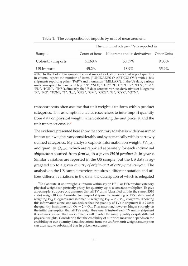
Table 1: The composition of imports by unit of measurement.

The unit in which quantity is reported in

Sample Count of items Kilograms and its derivatives Other Units

Colombia Imports 51.60% 38.57% 9.83%

US Imports 45.2% 18.9% 35.9%Note: In the Colombia sample the vast majority of shipments that report quantityin counts, report the number of items (“UNIDADES O ARTICULOS”) with a fewshipments reporting pairs (“PAR”) and thousands (“MILLAR”). In the US data, variousunits correspond to item count (e.g. “N”, “NO”, “DOZ”, “DPC”, “DPR”, “PCS”, “PRS”,“PK”, “HUN”, “THS”). Similarly, the US data contains various derivatives of kilograms:“K”, “KG”, “TON”, “T”, “kg”, “GRS”, “GM”, “GKG”, “G”, “CYK”, “GTN”.

transport costs often assume that unit weight is uniform within productcategories. This assumption enables researchers to infer import quantityfrom data on physical weight, when calculating the unit price, p, and theunit transport cost, τ.9

The evidence presented here show that contrary to what is widely-assumed,import unit weights vary considerably and systematically within narrowly-defined categories. My analysis exploits information on weight,W s,ωht,and quantity, Qs,ωht, which are reported separately for each individualshipment s sourced from firm ω, in a given HS10 product h, in year t.Similar variables are reported in the US sample, but the US data is ag-gregated up to a given country of origin–port of entry–product–year. Theanalysis on the US sample therefore requires a different notation and uti-lizes different variations in the data; the description of which is relegated

9To elaborate, if unit weight is uniform within say an HS10 or HS6 product category,physical weight can perfectly proxy for quantity up to a constant multiplier. To givean example, suppose one assumes that all TV units (classified within the same HS10code) weigh 10 kgs. Consider two import shipments consisting of TVs: shipment AweighingWA kilograms and shipment B weighingWB = 2×WA kilograms. Knowingthis information alone, one can deduce that the quantity of TVs in shipment B is 2-timesthe quantity in shipment A: QB = 2×QA. This assertion, however, hinges strongly onthe initial assumption that all TVs weigh the same. If instead each TV unit in shipmentB is 2-times heavier, the two shipments will involve the same quantity despite differentphysical weights. Considering that the credibility of our price measure depends on thecredibility of our quantity data, deviations from the uniform unit weight assumptioncan thus lead to substantial bias in price measurement.

11

to Appendix A.10 But one should bear in mind that while I occasionallyreport evidence from both data sets, I present the empirical strategy basedsolely on the transaction-level Colombia data described earlier.

Given the information on total weight and quantity, one can calculate theunit weight associated with shipment s, ωht as:

wgts,ωht =W s,ωht

Qs,ωht.

An elementary analysis of import unit weights uncovers four basic factsthat underlie both samples. Importantly, while I confine my benchmarkanalysis to import transactions reporting quantity in counts, the docu-mented facts apply more broadly. The only exception are import trans-actions that report quantity in some derivative of kilograms. For suchobservations (which constitute less than 19% of US imports, for example)unit weight is by definition “one” and import quantity is exactly equalto import weight: Qs,ωht ≡ Ws,ωht. For the remaining majority of im-port transactions, however, the variation in import unit weights are bothsubstantial and systematic.

FACT 1. Unit weights vary widely even within narrowly defined categories.

Table 2 reports the variation in import unit weights for various levels ofaggregation. Within the median country–product–year cell, the heaviest(95 percentile) item imported by Colombia is 18-times heavier than thelightest (5 percentile) item. The variation in import unit weights remainsignificant even across shipments from the same firm, of the same prod-uct, in the same year. A similar pattern is also visible in the US data,where within the median year–port of entry–product cell, the heaviest (95percentile) imported item weighs 16-times more than the lightest (5thpercentile) item.11

10The US sample reports the quantity (Qs,ωht) and weight (Ws,ωht) of aggregate im-ports from country s to US district ω, in a given HS10 product h, in year t. Therefore,while s indexes individual shipments in the benchmark analysis (conducted on theColombia sample) it denotes exporting country in the US data. Similarly, ω indexes anexporting firm in the benchmark analysis, whereas it indexes the port-of-entry in the USdata.

11Two clarifications about this and others statistic reported in Table 2 with relation

12

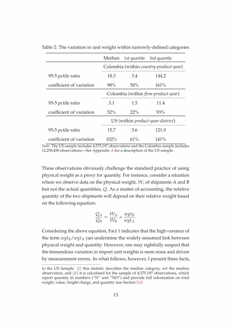
Table 2: The variation in unit weight within narrowly-defined categories

Median 1st quartile 3rd quartile

Colombia (within country-product-year)

95-5 pctile ratio 18.3 3.4 144.2

coefficient of variation 98% 50% 161%

Colombia (within firm-product-year)

95-5 pctile ratio 3.1 1.5 11.4

coefficient of variation 52% 22% 93%

US (within product-year-district)

95-5 pctile ratio 15.7 3.6 121.9

coefficient of variation 102% 61% 141%Note: The US sample includes 4,575,197 observations and the Colombia sample includes12,258,450 observations—See Appendix A for a description of the US sample.

These observations obviously challenge the standard practice of usingphysical weight as a proxy for quantity. For instance, consider a situationwhere we observe data on the physical weight,W , of shipments A and Bbut not the actual quantities, Q. As a matter of accounting, the relativequantity of the two shipments will depend on their relative weight basedon the following equation:

QA

QB=WA

WB× wgtB

wgtA.

Considering the above equation, Fact 1 indicates that the high variance ofthe term wgtB/wgtA can undermine the widely-assumed link betweenphysical weight and quantity. However, one may rightfully suspect thatthe tremendous variation in import unit weights is mere noise and drivenby measurement errors. In what follows, however, I present three facts,

to the US Sample: (i) this statistic describes the median category, not the medianobservation, and (ii) it is calculated for the sample of 4,575,197 observations, whichreport quantity in numbers (“N” and “NO”) and provide full information on totalweight, value, freight charge, and quantity (see Section 3.1)

13

each indicating that the variation in unit weights are systematic.

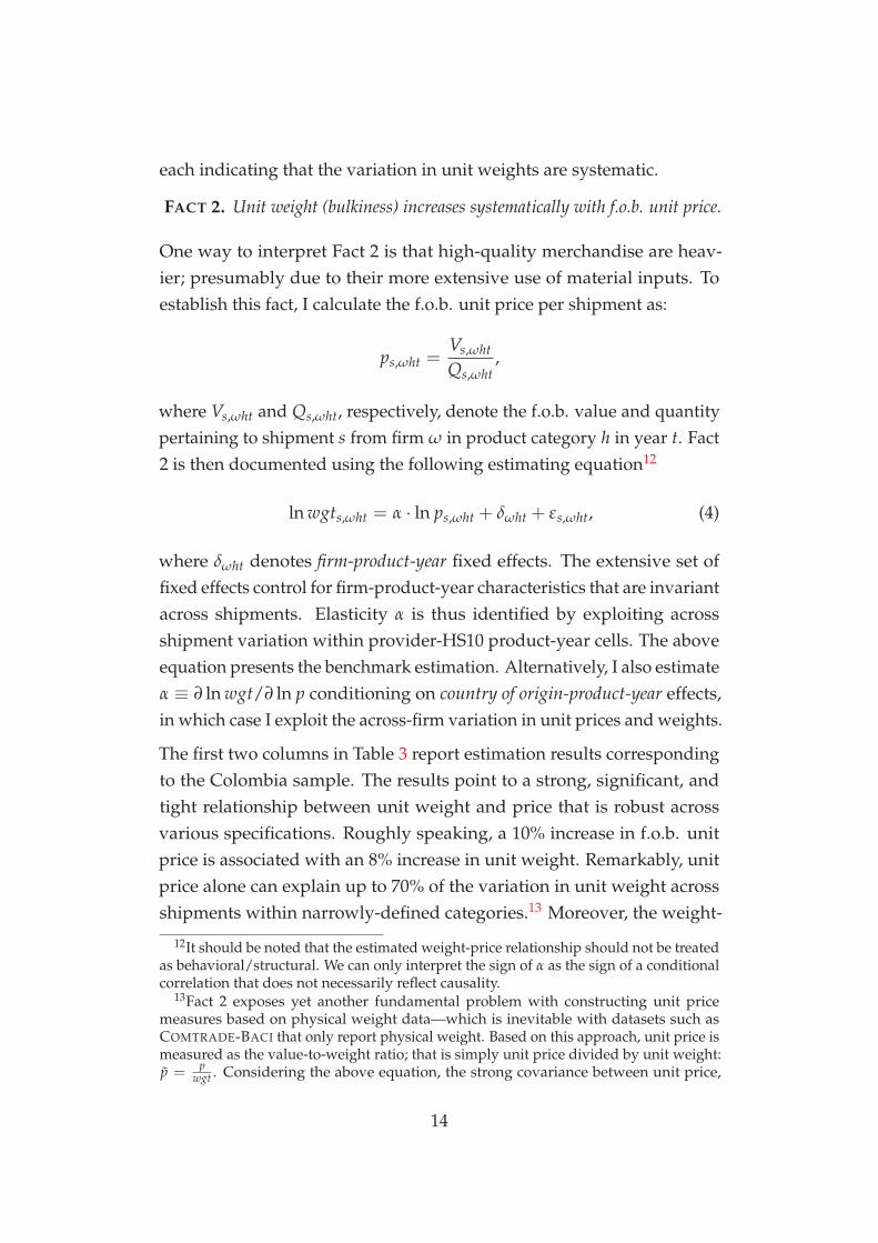
FACT 2. Unit weight (bulkiness) increases systematically with f.o.b. unit price.

One way to interpret Fact 2 is that high-quality merchandise are heav-ier; presumably due to their more extensive use of material inputs. Toestablish this fact, I calculate the f.o.b. unit price per shipment as:

ps,ωht =Vs,ωht

Qs,ωht,

where Vs,ωht and Qs,ωht, respectively, denote the f.o.b. value and quantitypertaining to shipment s from firm ω in product category h in year t. Fact2 is then documented using the following estimating equation12

ln wgts,ωht = α · ln ps,ωht + δωht + εs,ωht, (4)

where δωht denotes firm-product-year fixed effects. The extensive set offixed effects control for firm-product-year characteristics that are invariantacross shipments. Elasticity α is thus identified by exploiting acrossshipment variation within provider-HS10 product-year cells. The aboveequation presents the benchmark estimation. Alternatively, I also estimateα ≡ ∂ ln wgt/∂ ln p conditioning on country of origin-product-year effects,in which case I exploit the across-firm variation in unit prices and weights.

The first two columns in Table 3 report estimation results correspondingto the Colombia sample. The results point to a strong, significant, andtight relationship between unit weight and price that is robust acrossvarious specifications. Roughly speaking, a 10% increase in f.o.b. unitprice is associated with an 8% increase in unit weight. Remarkably, unitprice alone can explain up to 70% of the variation in unit weight acrossshipments within narrowly-defined categories.13 Moreover, the weight-

12It should be noted that the estimated weight-price relationship should not be treatedas behavioral/structural. We can only interpret the sign of α as the sign of a conditionalcorrelation that does not necessarily reflect causality.

13Fact 2 exposes yet another fundamental problem with constructing unit pricemeasures based on physical weight data—which is inevitable with datasets such asCOMTRADE-BACI that only report physical weight. Based on this approach, unit price ismeasured as the value-to-weight ratio; that is simply unit price divided by unit weight:p = p

wgt . Considering the above equation, the strong covariance between unit price,

14

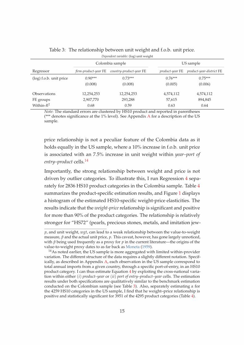
Table 3: The relationship between unit weight and f.o.b. unit price.Dependent variable: (log) unit weight

Colombia sample US sample

Regressor firm-product-year FE country-product-year FE product-year FE product-year-district FE

(log) f.o.b. unit price 0.90*** 0.73*** 0.76*** 0.75***(0.008) (0.008) (0.005) (0.006)

Observations 12,254,253 12,254,253 4,574,112 4,574,112FE groups 2,907,770 293,288 57,615 894,845Within-R2 0.68 0.59 0.63 0.64

Note: The standard errors are clustered by HS10 product and reported in parentheses(*** denotes significance at the 1% level). See Appendix A for a description of the USsample.

price relationship is not a peculiar feature of the Colombia data as itholds equally in the US sample, where a 10% increase in f.o.b. unit priceis associated with an 7.5% increase in unit weight within year–port ofentry–product cells.14

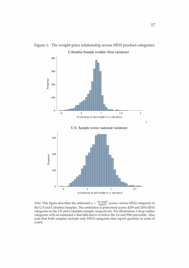
Importantly, the strong relationship between weight and price is notdriven by outlier categories. To illustrate this, I run Regression 4 sepa-rately for 2836 HS10 product categories in the Colombia sample. Table 4summarizes the product-specific estimation results, and Figure 1 displaysa histogram of the estimated HS10-specific weight-price elasticities. Theresults indicate that the weight-price relationship is significant and positivefor more than 90% of the product categories. The relationship is relativelystronger for “HS72” (pearls, precious stones, metals, and imitation jew-

p, and unit weight, wgt, can lead to a weak relationship between the value-to-weightmeasure, p and the actual unit price, p. This caveat, however, has gone largely unnoticed,with p being used frequently as a proxy for p in the current literature—the origins of thevalue-to-weight proxy dates to as far back as Moneta (1959).

14As noted earlier, the US sample is more aggregated with limited within-providervariation. The different structure of the data requires a slightly different notation. Specif-ically, as described in Appendix A, each observation in the US sample correspond tototal annual imports from a given country, through a specific port-of-entry, in an HS10product category. I can thus estimate Equation 4 by exploiting the cross-national varia-tion within either (i) product–year or (ii) port of entry–product–year cells. The estimationresults under both specifications are qualitatively similar to the benchmark estimationconducted on the Colombian sample (see Table 3). Also, separately estimating α forthe 4259 HS10 categories in the US sample, I find that he weight–price relationship ispositive and statistically significant for 3951 of the 4295 product categories (Table 4).

15

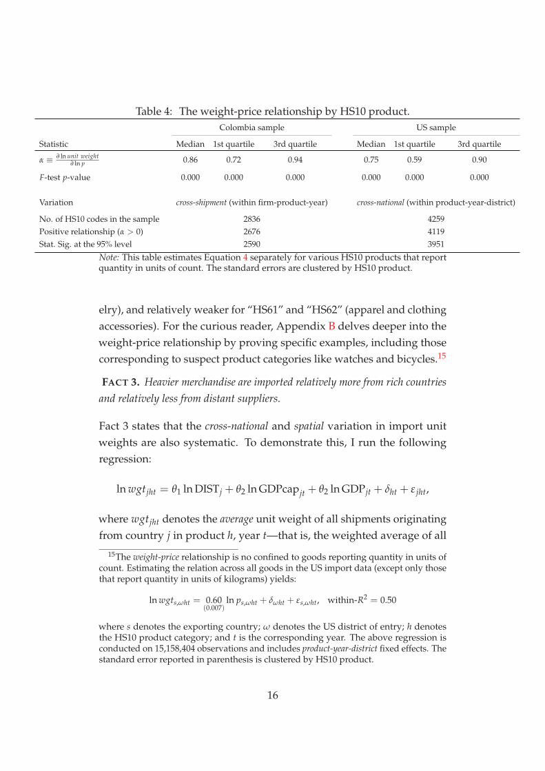
Table 4: The weight-price relationship by HS10 product.Colombia sample US sample

Statistic Median 1st quartile 3rd quartile Median 1st quartile 3rd quartile

α ≡ ∂ ln unit weight∂ ln p 0.86 0.72 0.94 0.75 0.59 0.90

F-test p-value 0.000 0.000 0.000 0.000 0.000 0.000

Variation cross-shipment (within firm-product-year) cross-national (within product-year-district)

No. of HS10 codes in the sample 2836 4259Positive relationship (α > 0) 2676 4119Stat. Sig. at the 95% level 2590 3951

Note: This table estimates Equation 4 separately for various HS10 products that reportquantity in units of count. The standard errors are clustered by HS10 product.

elry), and relatively weaker for “HS61” and “HS62” (apparel and clothingaccessories). For the curious reader, Appendix B delves deeper into theweight-price relationship by proving specific examples, including thosecorresponding to suspect product categories like watches and bicycles.15

FACT 3. Heavier merchandise are imported relatively more from rich countriesand relatively less from distant suppliers.

Fact 3 states that the cross-national and spatial variation in import unitweights are also systematic. To demonstrate this, I run the followingregression:

ln wgtjht = θ1 ln DISTj + θ2 ln GDPcapjt + θ2 ln GDPjt + δht + ε jht,

where wgtjht denotes the average unit weight of all shipments originatingfrom country j in product h, year t—that is, the weighted average of all

15The weight-price relationship is no confined to goods reporting quantity in units ofcount. Estimating the relation across all goods in the US import data (except only thosethat report quantity in units of kilograms) yields:

ln wgts,ωht = 0.60(0.007)

ln ps,ωht + δωht + εs,ωht, within-R2 = 0.50

where s denotes the exporting country; ω denotes the US district of entry; h denotesthe HS10 product category; and t is the corresponding year. The above regression isconducted on 15,158,404 observations and includes product-year-district fixed effects. Thestandard error reported in parenthesis is clustered by HS10 product.

16

17

Figure 1: The weight-price relationship across HS10 product categories.

0

100

200

300

400

Fre

qu

ency

0 .5 1 1.5 2

α (elasticity of unit weight w.r.t. unit price)

Colombia Sample (within−firm variation)

.;

0

100

200

300

Fre

qu

ency

0 .5 1 1.5

α (elasticity of unit weight w.r.t. unit price)

U.S. Sample (cross−national variation)

Note: This figure describes the estimated α =ln weightln price across various HS10 categories in

the U.S and Colombia Samples. The estimation is preformed across 4259 and 2836 HS10categories in the US and Colombia sample, respectively. For illustration, I drop outliercategories with an estimated α that falls above or below the 1st and 99th percentile. Also,note that both samples include only HS10 categories that report quantity in units ofcount.

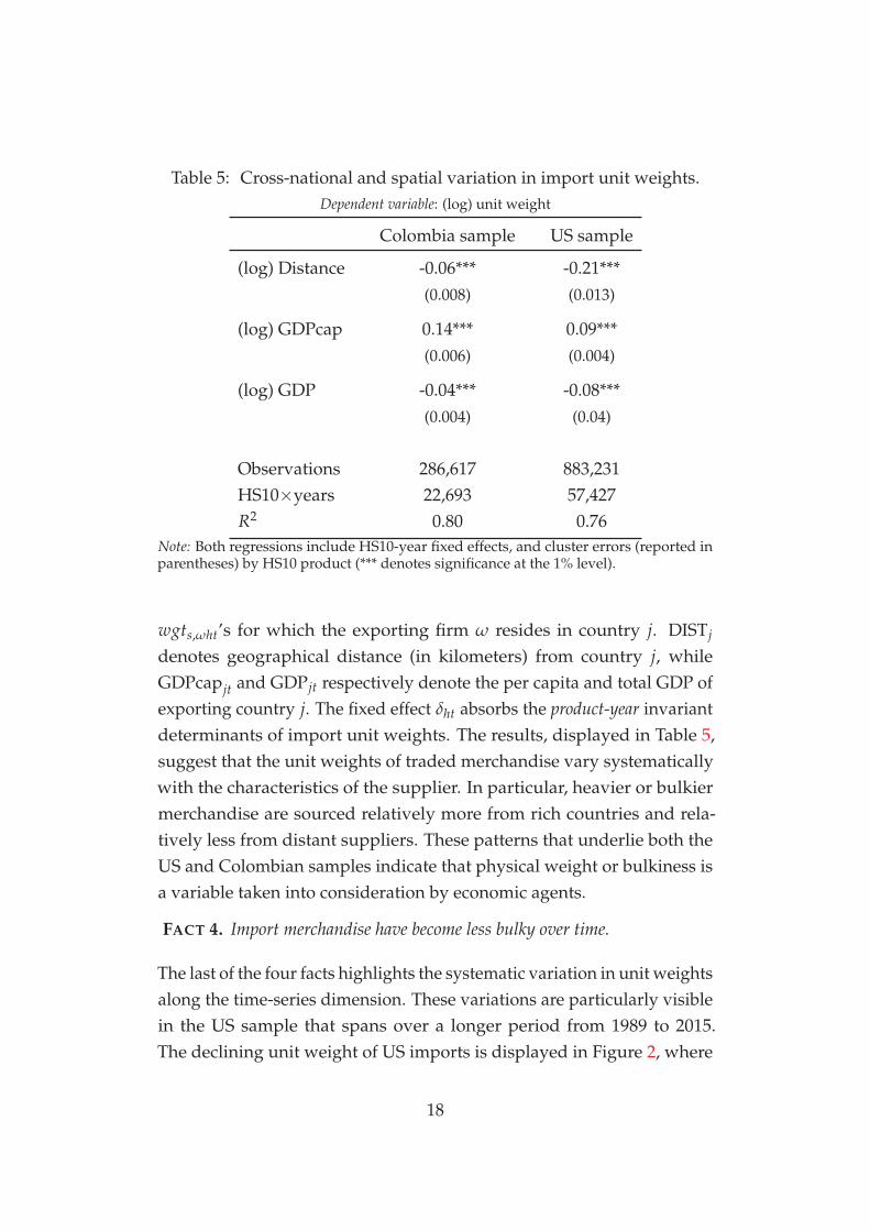
Table 5: Cross-national and spatial variation in import unit weights.Dependent variable: (log) unit weight


(log) Distance -0.06*** -0.21***(0.008) (0.013)

(log) GDPcap 0.14*** 0.09***(0.006) (0.004)

(log) GDP -0.04*** -0.08***(0.004) (0.04)

Observations 286,617 883,231HS10×years 22,693 57,427R2 0.80 0.76

Note: Both regressions include HS10-year fixed effects, and cluster errors (reported inparentheses) by HS10 product (*** denotes significance at the 1% level).

wgts,ωht’s for which the exporting firm ω resides in country j. DISTj

denotes geographical distance (in kilometers) from country j, whileGDPcapjt and GDPjt respectively denote the per capita and total GDP ofexporting country j. The fixed effect δht absorbs the product-year invariantdeterminants of import unit weights. The results, displayed in Table 5,suggest that the unit weights of traded merchandise vary systematicallywith the characteristics of the supplier. In particular, heavier or bulkiermerchandise are sourced relatively more from rich countries and rela-tively less from distant suppliers. These patterns that underlie both theUS and Colombian samples indicate that physical weight or bulkiness isa variable taken into consideration by economic agents.

FACT 4. Import merchandise have become less bulky over time.

The last of the four facts highlights the systematic variation in unit weightsalong the time-series dimension. These variations are particularly visiblein the US sample that spans over a longer period from 1989 to 2015.The declining unit weight of US imports is displayed in Figure 2, where

18

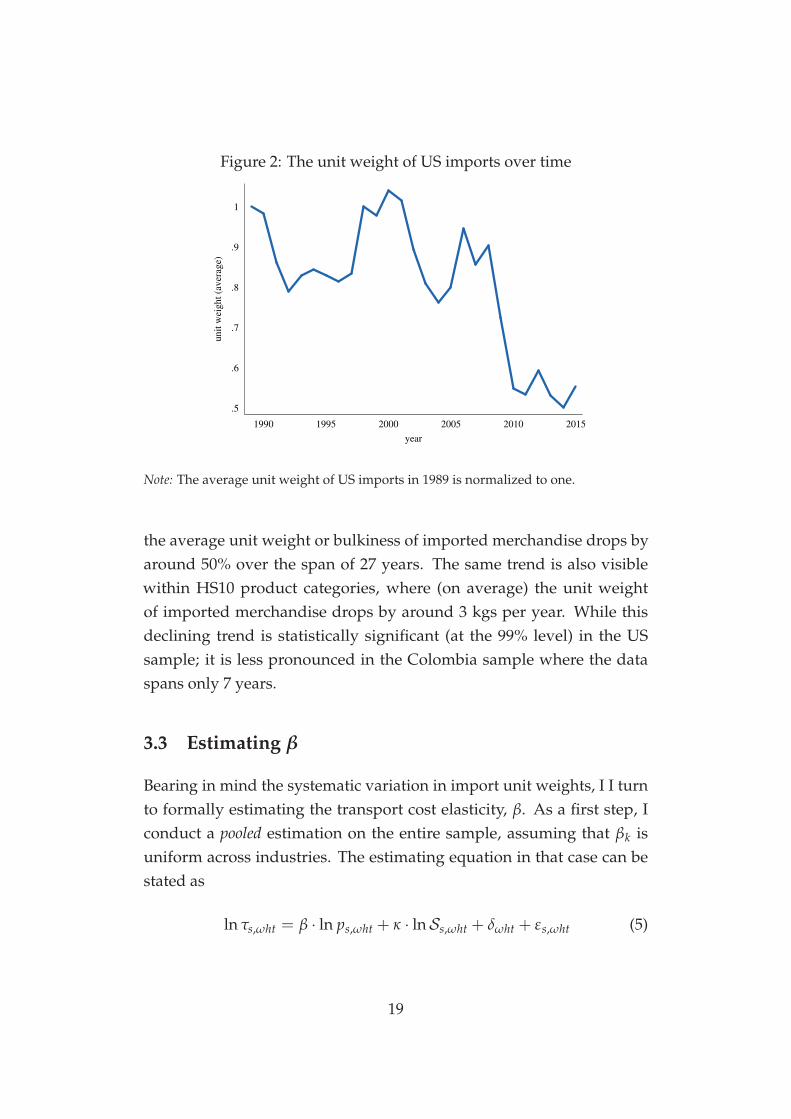
Figure 2: The unit weight of US imports over time

.5

.6

.7

.8

.9

1u

nit

wei

gh

t (a

ver

age)

1990 1995 2000 2005 2010 2015

year

Note: The average unit weight of US imports in 1989 is normalized to one.

the average unit weight or bulkiness of imported merchandise drops byaround 50% over the span of 27 years. The same trend is also visiblewithin HS10 product categories, where (on average) the unit weightof imported merchandise drops by around 3 kgs per year. While thisdeclining trend is statistically significant (at the 99% level) in the USsample; it is less pronounced in the Colombia sample where the dataspans only 7 years.

3.3 Estimating β

Bearing in mind the systematic variation in import unit weights, I I turnto formally estimating the transport cost elasticity, β. As a first step, Iconduct a pooled estimation on the entire sample, assuming that βk isuniform across industries. The estimating equation in that case can bestated as

ln τs,ωht = β · ln ps,ωht + κ · lnSs,ωht + δωht + εs,ωht (5)

19

where τs,ωht and ps,ωht respectively denote the unit transport cost and theunit price associated with observation s, ωht (shipment s–firm ω–producth–year t). The above formulation estimates β controlling for (i) provider-product-year fixed effects, δωht, and (ii) shipment scale, Ss,ωht, sinceinternational transportation may be subject to scale economies.16 Theremaining idiosyncratic error term, εs,ωht, reflects measurement error plusnon-systematic cost-shifters specific to shipment s, ωht.

In my benchmark estimation I fit Equation 5 to the universe of Colombianimport transactions, identifying β using the within firm-product-year vari-ation in τ and p. For comparison, I also estimate β using the country-levelUS import data, which has been used extensively in the prior literature.Given its highly aggregated nature, the US data permits the estimationof β based on only the cross-national variation in τ and p within HS10product categories—the details of which are relegated to Appendix A.

Parametrically, Equation 5 closely resembles the aggregate cost functionestimated by Hummels and Skiba (2004)—labeled as “Equation 10” in theirpaper. However, aside from being based on transaction-level (as opposedto country-level) data and controlling for firm fixed effects, my estimationstrategy differs from Hummels and Skiba (2004) in two key aspects: (i) Iformally control for the systematic variation in import unit weights, and(ii) I utilize detailed information on importer-exporter characteristics tohandle the simultaneity problem underlying the estimation of β. Below, Ielaborate on these two distinctive features.

Accounting for the Variation in Unit Weights. The traditional trans-port cost estimation employed by Hummels and Skiba (2004) and Hum-mels et al. (2009), among others, identifies β conditional on unit weightbeing uniform within product categories. Recall that this identifying

16I control for scale effects using the number of packages in shipment s, ωht. In-tuitively, shipping out ten boxes at once is more cost-efficient than sending out tensingle-box shipments throughout the year. When analyzing the US sample, I subscribeto the estimation strategy proposed by Hummels and Skiba (2004), which is reflectiveof the limited information available in the data set. In particular, I control for scalewith the total weight of all shipments aggregated into a given data entry, and employbilateral distance (DISTs) and the GDP per capita of the origin country as additionalcontrols—see Appendix A for a thorough description.

20

assumption is imposed in face of data limitations, as it allows researchersto infer the import quantity, Qs,ωht, from data on shipment weight,Ws,ωht.Put differently, the uniform unit weight assumption allows researcher toestimates β as the elasticity of transport cost per kg, τ ≡ τ

wgt with respectto the value per kg, p = p

wgt of the traded goods.

The traditional approach can be formally described by re-writing theestimating Equation 5 in terms of τ ≡ τ

wgt and p = pwgt :

ln τs,ωht = β · ln ps,ωht + κ · lnSs,ωht + δωht + (β− 1) ln wgts,ωht︸︷︷︸omitted variable

+εs,ωht

When unit weight is uniform within firm-product-year cells (i.e., wgts,ωht =

wgtωht), the omitted term is absorbed by the fixed effect, δωht, and the tra-ditional approach delivers an unbiased estimate of β. Factually, however,not only is wgt non-uniform, but it is negatively correlated with value perkg, p. As a consequence, the traditional approach suffers from a classicalcase of omitted variable bias that attenuates β.

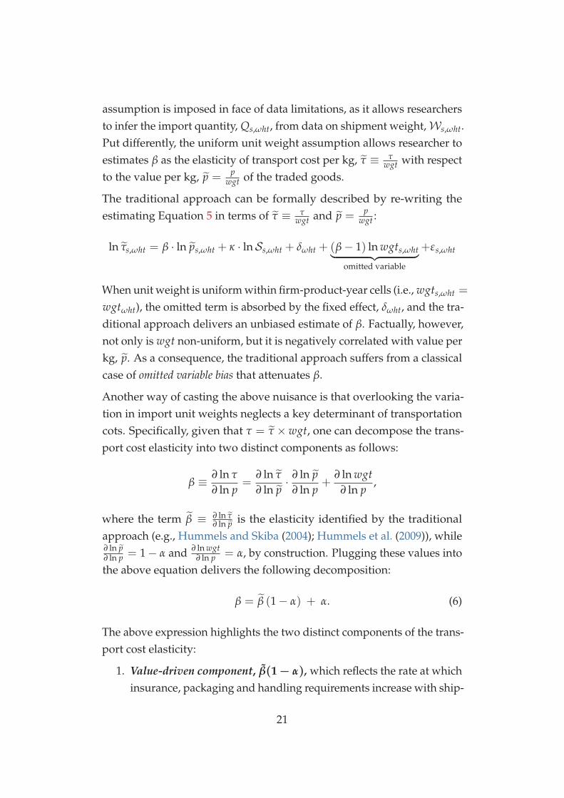
Another way of casting the above nuisance is that overlooking the varia-tion in import unit weights neglects a key determinant of transportationcots. Specifically, given that τ = τ × wgt, one can decompose the trans-port cost elasticity into two distinct components as follows:

β ≡ ∂ ln τ

∂ ln p=

∂ ln τ

∂ ln p· ∂ ln p

∂ ln p+

∂ ln wgt∂ ln p

,

where the term β ≡ ∂ ln τ∂ ln p is the elasticity identified by the traditional

approach (e.g., Hummels and Skiba (2004); Hummels et al. (2009)), while∂ ln p∂ ln p = 1− α and ∂ ln wgt

∂ ln p = α, by construction. Plugging these values intothe above equation delivers the following decomposition:

β = β (1− α) + α. (6)

The above expression highlights the two distinct components of the trans-port cost elasticity:

1. Value-driven component, β(1 − α), which reflects the rate at whichinsurance, packaging and handling requirements increase with ship-

21

ment value.

2. Weight-driven component, α, which accounts for the fact that high-priced items are heavier and, therefore, costlier to transport.

Considering the above decomposition, conditional on unit weight beinguniform (i.e., α = 0), the transport cost elasticity equals β, which is theelasticity estimated under the traditional approach. However, in practice,given that α ≈ 0.75, the traditional approach delivers a systematicallyattenuated elasticity estimate, β = β−α

1−α < β.

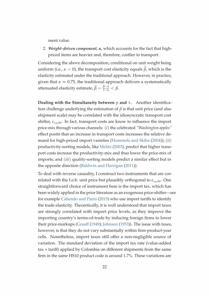
Dealing with the Simultaneity between p and τ. Another identifica-tion challenge underlying the estimation of β is that unit price (and alsoshipment scale) may be correlated with the idiosyncratic transport costshifter, εs,ωht. In fact, transport costs are know to influence the importprice-mix through various channels: (i) the celebrated “Washington apples”effect posits that an increase in transport costs increases the relative de-mand for high-priced import varieties (Hummels and Skiba (2004)); (ii)productivity-sorting models, like Melitz (2003), predict that higher trans-port costs increase the productivity-mix and thus lower the price-mix ofimports; and (iii) quality-sorting models predict a similar effect but inthe opposite direction (Baldwin and Harrigan (2011)).

To deal with reverse causality, I construct two instruments that are cor-related with the f.o.b. unit price but plausibly orthogonal to εs,ωht. Onestraightforward choice of instrument here is the import tax, which hasbeen widely applied in the prior literature as an exogenous price-shifter—seefor example Caliendo and Parro (2015) who use import tariffs to identifythe trade elasticity. Theoretically, it is well understood that import taxesare strongly correlated with import price levels, as they improve theimporting country’s terms-of-trade by inducing foreign firms to lowertheir price-markups (Graaff (1949); Johnson (1953)). The issue with taxes,however, is that they do not vary substantially within firm-product-yearcells. Nonetheless, import taxes still offer a non-negligible source ofvariation. The standard deviation of the import tax rate (value-addedtax + tariff) applied by Colombia on different shipments from the samefirm in the same HS10 product code is around 1.7%. These variations are

22

prompted by the fact that (i) a different value-added tax rate may applyto different shipments pertaining to the same firm-product-year category,and (ii) import tariff rates vary over time due to trade agreements orWTO disputes and settlements (see Eaton et al. (2010)).

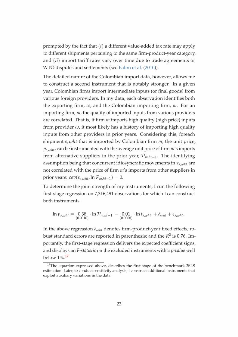
The detailed nature of the Colombian import data, however, allows meto construct a second instrument that is notably stronger. In a givenyear, Colombian firms import intermediate inputs (or final goods) fromvarious foreign providers. In my data, each observation identifies boththe exporting firm, ω, and the Colombian importing firm, m. For animporting firm, m, the quality of imported inputs from various providersare correlated. That is, if firm m imports high quality (high price) inputsfrom provider ω, it most likely has a history of importing high qualityinputs from other providers in prior years. Considering this, foreachshipment s, ωht that is imported by Colombian firm m, the unit price,ps,ωht, can be instrumented with the average unit price of firm m’s importsfrom alternative suppliers in the prior year, Pm,ht−1. The identifyingassumption being that concurrent idiosyncratic movements in τs,ωht arenot correlated with the price of firm m’s imports from other suppliers inprior years: cov(εs,ωht, lnPm,ht−1) = 0.

To determine the joint strength of my instruments, I run the followingfirst-stage regression on 7,316,491 observations for which I can constructboth instruments:

ln ps,ωht = 0.38(0.0010)

· lnPm,ht−1 − 0.01(0.0008)

· ln ts,ωht + δωht + εs,ωht.

In the above regression δωht denotes firm-product-year fixed effects; ro-bust standard errors are reported in parenthesis; and the R2 is 0.76. Im-portantly, the first-stage regression delivers the expected coefficient signs,and displays an F-statistic on the excluded instruments with a p-value wellbelow 1%.17

17The equation expressed above, describes the first stage of the benchmark 2SLSestimation. Later, to conduct sensitivity analysis, I construct additional instruments thatexploit auxiliary variations in the data.

23

3.4 Estimation Results

The benchmark estimation results are displayed in Table 6. For com-parison, the table also reports ordinary least square (OLS) estimates ofthe transport cost elasticity, which maybe upward biased due to the si-multaneity between τ and p. Encouragingly, the two-stage least square(2SLS) estimator delivers lower estimates of β than the OLS estimator,which indicates that the IV approach is correcting the bias inflicted bythe simultaneity problem. As expected, the corrective power of the IVapproach is considerably less in the case of the less-detailed and highlyaggregated US data.

In summary, my preferred estimate for the transport cost elasticity isβ = 0.84, which though higher than traditional estimates, rejects theexact iceberg (β = 1) specification. The estimation results also confirmthe prevalence of scale effects in transportation, whereby a 10% increasein shipment scale reduces the unit shipping cost by 1.3% across variousvarious specifications.18

To put my estimates in perspective, I also estimate β using the traditionalapproach of regressing τ = τ/wgt on p = p/wgt. As noted earlier,this widely-used approach delivers attenuated estimates of β due to anomitted variable bias. The results arising from the traditional approachare reported in Table 7 and, as projected, point to a systematically lowerelasticity, β ≈ 0.4. To dig deeper, the difference between the traditionalestimation and the benchmark estimation is that the latter accounts forthe role of product weight in transportation. Following Equation 6, thetransport cost elasticity, β ≡ d ln τ

d ln p , is composed of a weight-driven com-

ponent, α, and a value-driven component, β (1− α). Noting that β ≈ 0.4

18The estimation conducted on the US sample (which exploits across country vari-ations) confirms two well-established results: (i) Distance matters. A 10% increase ingeographical distance to the US increases the transport cost by more than 2.4%, and (ii)High-income countries face systematically lower transport costs. Specifically, high-incomecountries are significantly more efficient in transportation, and face lower costs despitepaying higher wages.

24

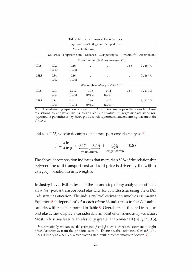
Table 6: Benchmark EstimationDependent Variable: (log) Unit Transport Cost

Variables (in logs)

Unit Price Shipment Scale Distance GDP per capita within-R2 Observations

Colombia sample (firm-product-year FE)

OLS 0.92 -0.16 ... ... 0.63 7,316,491(0.000) (0.000)

2SLS 0.84 -0.16 ... ... ... 7,316,491(0.002) (0.000)

US sample (product-year-district FE)

OLS 0.91 -0.012 0.10 -0.11 0.69 3,341,703(0.000) (0.000) (0.002) (0.001)

2SLS 0.88 -0.014 0.09 -0.10 ... 3,341,703(0.001) (0.001) (0.002) (0.001)

Note: The estimating equation is Equation 5. All 2SLS estimates pass the over-identifyingrestrictions test and have low first-stage F-statistic p-values. All regressions cluster errors(reported in parentheses) by HS10 product. All reported coefficient are significant at the1% level.

and α ≈ 0.75, we can decompose the transport cost elasticity as19

β ≡ d ln τ

d ln p≈ 0.4(1− 0.75)︸︷︷︸

value-driven

+ 0.75︸︷︷︸weight-driven

= 0.85

The above decomposition indicates that more than 80% of the relationshipbetween the unit transport cost and unit price is driven by the within-category variation in unit weights.

Industry-Level Estimates. In the second step of my analysis, I estimatean industry-level transport cost elasticity for 33 industries using the GTAPindustry classification. The industry-level estimation involves estimatingEquation 5 independently for each of the 33 industries in the Colombiasample, with results reported in Table 8. Overall, the estimated transportcost elasticities display a considerable amount of cross-industry variation.Most industries feature an elasticity greater than one-half (i.e., β > 0.5),

19Alternatively, we can use the estimated β and β to cross-check the estimated weight-price elasticity, α, from the previous section. Doing so, the estimated β ≈ 0.84 andβ ≈ 0.4 imply an α ≈ 0.75, which is consistent with direct estimates in Section 3.2.

25

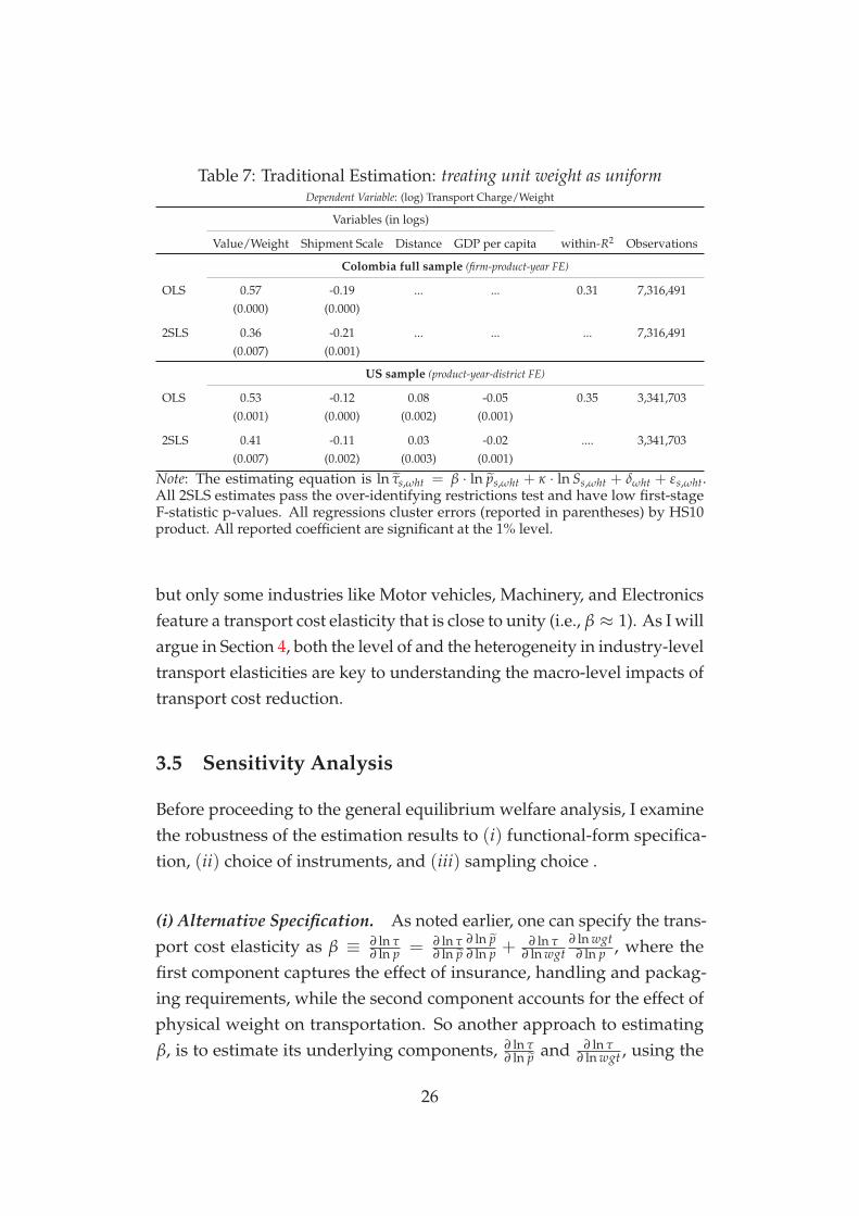
Table 7: Traditional Estimation: treating unit weight as uniformDependent Variable: (log) Transport Charge/Weight

Variables (in logs)

Value/Weight Shipment Scale Distance GDP per capita within-R2 Observations

Colombia full sample (firm-product-year FE)

OLS 0.57 -0.19 ... ... 0.31 7,316,491(0.000) (0.000)

2SLS 0.36 -0.21 ... ... ... 7,316,491(0.007) (0.001)

US sample (product-year-district FE)

OLS 0.53 -0.12 0.08 -0.05 0.35 3,341,703(0.001) (0.000) (0.002) (0.001)

2SLS 0.41 -0.11 0.03 -0.02 .... 3,341,703(0.007) (0.002) (0.003) (0.001)

Note: The estimating equation is ln τs,ωht = β · ln ps,ωht + κ · ln Ss,ωht + δωht + εs,ωht.All 2SLS estimates pass the over-identifying restrictions test and have low first-stageF-statistic p-values. All regressions cluster errors (reported in parentheses) by HS10product. All reported coefficient are significant at the 1% level.

but only some industries like Motor vehicles, Machinery, and Electronicsfeature a transport cost elasticity that is close to unity (i.e., β ≈ 1). As I willargue in Section 4, both the level of and the heterogeneity in industry-leveltransport elasticities are key to understanding the macro-level impacts oftransport cost reduction.

3.5 Sensitivity Analysis

Before proceeding to the general equilibrium welfare analysis, I examinethe robustness of the estimation results to (i) functional-form specifica-tion, (ii) choice of instruments, and (iii) sampling choice .

(i) Alternative Specification. As noted earlier, one can specify the trans-port cost elasticity as β ≡ ∂ ln τ

∂ ln p = ∂ ln τ∂ ln p

∂ ln p∂ ln p + ∂ ln τ

∂ ln wgt∂ ln wgt

∂ ln p , where thefirst component captures the effect of insurance, handling and packag-ing requirements, while the second component accounts for the effect ofphysical weight on transportation. So another approach to estimatingβ, is to estimate its underlying components, ∂ ln τ

∂ ln p and ∂ ln τ∂ ln wgt , using the

26

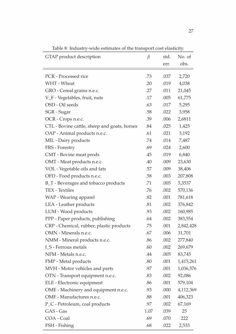
27

Table 8: Industry-wide estimates of the transport cost elasticity.

GTAP product description β std.err.

No. ofobs.

PCR - Processed rice .73 .037 2,720WHT - Wheat .20 .019 4,038GRO - Cereal grains n.e.c. .27 .011 21,045V_F - Vegetables, fruit, nuts .17 .005 61,775OSD - Oil seeds .63 .017 5,295SGR - Sugar .58 .022 3,958OCR - Crops n.e.c. .39 .006 2,6811CTL - Bovine cattle, sheep and goats, horses .84 .025 1,425OAP - Animal products n.e.c. .61 .021 3,192MIL - Dairy products .74 .014 7,487FRS - Forestry .69 .024 2,600CMT - Bovine meat prods .45 .019 6,840OMT - Meat products n.e.c. .40 .009 23,630VOL - Vegetable oils and fats .57 .009 38,406OFD - Food products n.e.c. .58 .003 207,808B_T - Beverages and tobacco products .71 .005 5,3537TEX - Textiles .76 .002 570,136WAP - Wearing apparel .82 .001 781,618LEA - Leather products .81 .002 376,842LUM - Wood products .93 .002 160,985PPP - Paper products, publishing .64 .002 383,554CRP - Chemical, rubber, plastic products .75 .001 2,842,428OMN - Minerals n.e.c. .67 .006 31,701NMM - Mineral products n.e.c. .86 .002 277,840I_S - Ferrous metals .60 .002 269,679NFM - Metals n.e.c. .44 .005 83,745FMP - Metal products .80 .001 1,415,261MVH - Motor vehicles and parts .97 .001 1,036,576OTN - Transport equipment n.e.c. .83 .002 92,086ELE - Electronic equipment .86 .001 579,104OME - Machinery and equipment n.e.c. .93 .000 4,112,369OMF - Manufactures n.e.c. .88 .001 406,323P_C - Petroleum, coal products .97 .002 67,169GAS - Gas 1.07 .039 25COA - Coal .69 .070 222FSH - Fishing .68 .022 2,533

following equation:

ln τs,ωht = 0.96(.0004)

ln ps,ωht + 0.54(.0002)

ln wgts,ωht− 0.17(.0002)

lnSs,ωht + δωht + εs,ωht.

So given that (i) ∂ ln τ∂ ln p = 0.54 and ∂ ln τ

∂ ln wgt = 0.96, plus (ii) ∂ ln p∂ ln p = 1− α ≈

0.25 and ∂ ln wgt∂ ln p = α ≈ 0.75, we can calculate β as follows:

β ≡ ∂ ln τ

∂ ln p=

∂ ln τ

∂ ln p· (1− α) +

∂ ln τ

∂ ln wgt· α ≈ 0.85

Encouragingly, the above approach estimates an elasticity that is verysimilar to the benchmark estimation. On a related note, my estimationof β is agnostic to the parametric structure of the transport cost function.Several studies have meanwhile have assumed the parametrization τ =

νp + f , where ν and f denote the multiplicative and additive componentsof the transport cost. In Appendix D, I use Monte-Carlo simulationto show how different ratios of ν/ f map into different transport costelasticity values.

(ii) Choice of Instruments. To verify the robustness of the benchmarkresults to the choice of instruments, I perform the estimation with an alter-native instrument for f.o.b. unit price. The alternative instrument buildson the observation that a considerable fraction of imports are conductedby Colombian firms that concurrently engage in export activity. Thereis also accumulating evidence that Colombian firms that import high-quality inputs, produce and export higher quality outputs (Kugler andVerhoogen (2012)). Guided by this regularity, I first merge the Colombianimport and export databases by matching importer and exporter ids. Thisleaves me with a subsample of import transactions conducted by Colom-bian firms that engage in both importing and exporting activities withina product category. In this subsample, each shipment is imported by aColombian firm, m, for which I can calculate the average f.o.b. unit priceof exports,P x

mht. I then instrument for the f.o.b. unit price of shipments, ωht, ps,ωht, with the lagged export price of the Colombian importingfirm, P x

mht−1. This approach basically exploits the across shipment vari-

28

ation in the quality of the Colombian importing partner to identify thetransport cost elasticity. The estimation results, which are presented inthe Table 12 still reject the exact-iceberg specification but point to a lowerelasticity—this may be driven by the fact the subsample I can constructP x

mht for is considerably smaller than the original sample.

(iii) Sampling Choice. In compliance with the existing literature, mybenchmark analysis dropped transactions that report quantity in units ofkilogram (e.g., transactions relating to commodities such as coal, metals,wheat, etc.). As an additional check, I re-estimate the transport costelasticity using the full sample of observation including those that reportquantity in kilograms. The results reported in Table 12 point to a transportcost elasticity of β = 0.8, which is very similar to the benchmark estimate.

Another common concern with micro-level trade data is the prevalence ofmeasurement errors. In light of such concerns, I re-estimate the transportcost elasticity using a trimmed sample of Colombian imports that excludestransactions reporting imports value smaller than 1000 US dollars. Such atrim presumably eliminates many suspect observations that are contami-nated with measurement errors. Encouragingly, the estimation performedon the trimmed sample delivers estimates that remain within a standarderror of the benchmark results—see Table 12.

3.6 Discussion

While my estimation rejects the exact-iceberg specification, it also suggeststhat in most industries transport costs are quasi-iceberg. One, however,should exercise caution when interpreting these results. In particular, thefinding that transport costs are quasi-iceberg does not undermine the con-clusion of Hummels and Skiba (2004) that the Alchian-Allen forces are em-pirically significant. Even small deviations from the iceberg specificationcan trigger the Alchian-Allen mechanism. Instead, the quasi-iceberg spec-ification suggests that the Alchian-Allen forces may be slightly weakerthan previously thought, bringing to attention other competing forcessuch as quality-sorting (Baldwin and Harrigan (2011); Crozet et al. (2012))

29

or markup specialization (Lashkaripour (2015)).20 Also, note that thepresent analysis is focused solely on transportation costs. There are othertypes of trade barriers, many of which are non-tangible such as red tapes.Hence, one should exercise caution in extrapolating the above resultsto other types of trade barriers. Irarrazabal et al. (2014) and Cosar andDemir (2017) have developed indirect methodologies that can identify thenon-tangible trade cost elasticity. The trade-off is that in these alternativemethodologies, identification relies on stronger parametric assumptionsabout the (i) transport cost function, (ii) import demand function, and(iii) general equilibrium structure of the economy.

4 The Gains from Transport Cost Reduction

As a final step, I use the micro-estimated transport cost elasticities toquantify the gains from international transport cost reduction. My anal-ysis here involves plugging the estimated industry-level transport costelasticities into a general equilibrium, multi-country model of interna-tional trade. I then calibrate this model to trade data and use it to performcounterfactual welfare analyses. I am particularly interested in determin-ing how normalizing the transport cost elasticity to “one,” affects thecredibility of counterfactual predictions.

Before proceeding to the actual analysis, let me briefly describe how itrelates to standard welfare analyses often performed in the literature. Tothis end, consider a special case of the model presented in Section 2, wheretransportation services are supplied subject to perfect competition and arecostlessly traded. Transporting the final goods is meanwhile costly andpaid in terms of transportation services. Assigning transportation serviceas the numeraire, the cost of transporting the final goods produced by firmω, located in country j, to market i is τωi,k = tji,k f (pωi,k). I assume thatthe transportation sector is large enough so that the wage rate in country iis pinned down by its transportation productivity: wi = zi. Additionally,

20There is also the pricing-to-market mechanism, which according to Hummels andSkiba (2004) is too weak to explain the large price-distance elasticity by itself.

30

I assume that the utility aggregator across final good industries is Cobb-Douglas or CES so that ∂ ln Vi

∂ ln Yi= 1.

Within the above framework, one can think of a range of counterfactualpolicy experiments that correspond to declining transport costs (e.g., adecline in zi or tji,k). I will focus on the most basic experiment, whichis analyzing the welfare consequences of improving a country’s trans-portation efficiency, zi. Following the discussion in Section 2, the welfareeffects of such a development can be calculated as follows

d ln Wi =

1−∑k

∑ω∈Ωi,k

λωi,k [sωi,kβk + (1− sωi,k)]

d ln zi, (7)

where λωi,k denotes the share of country i’s expenditure spent on firmω varieties from industry k; and sωi,k ≡ τωi,k/πωi,k is the variety-specificshare of transport costs in the final price.21 Under the widely-assumednormalization, βk = 1, Equation 7 merely reduces to

d ln Wi = (1− λii) d ln zi.

The above formula incapsulates the basic insight in the Arkolakis et al.(2012) formula or in the exact hat-algebra methodology popularized byDekle et al. (2007). That is, we can compute the welfare gains from animprovement in transportation infrastructure, knowing only a region’smacro-level import-to-GDP ratio. Compare this with Equation 7, wherethe implied welfare gains depend not only on macro-level import sharesbut also on the entire schedule of local micro-level prices.

With the above discussion in mind, I now use actual trade data to evaluated ln Wi in response to a 10% increase in transportation efficiency—i.e.,d ln zi = 0.1. My primary goal is to determine how sensitive the computedwelfare impacts are to the normalization of βk to one.

21The above expression is derived noting that

d ln Wi = d ln Yi −∑k

∑ω∈Ωi,k

λωi,kd ln πωi,k,

where d ln Yi = d ln wi = d ln zi and d ln πωi,k = [sωi,kβk + (1− sωi,k)] dzi if ω ∈ Ωi,k.

31

To conduct my analysis, I use industry-level trade, production, and ex-penditure data for 7 regions and 33 industry. My main data source isthe widely-used Global Trade Analysis Project database (GTAP 8). Theregions included in the analysis are Brazil, China, the European Union,India, Japan, the United States, and the Rest of the World. These regionsare chosen to represent countries form different income levels. The 33industries included in the analysis are listed in Table 8, and span theagricultural and manufacturing sectors of the economy.

It should be clear by now that because βk is strictly different from “one”in all industries, I cannot apply the hat-algebra methodology to conductmy counterfactual policy analysis. Instead, I have to calibrate the modelto the global matrix of industry-level trade, production, and expenditureshares. Ideally, one may use data on the universes of firm-level sales andprices to determine λωi,k and sωi,k. However, currently, such a rich data isfar from accessible. As a workaround, I treat each region as one integratedsupplier when evaluating Equation 8. In that case, d ln Wi depends onβk’s and the industry and regional-level trade and transport cost shares,λji,k and sji,k, as follows:

d ln Wi =

(1−∑

kλii,k [sii,kβk + (1− sii,k)]

)d ln zi.

In the above expression λii,k is directly observable, but I need to calibratethe industry-level transport cost share, sii,k. Using the parameterizationτji,k = tji,k pβk

j,k, and given that sji,k =τji,k

pj,k+τji,k, I need the vector of f.o.b.

price levels,

pj,k

, and the matrix of transport cost shifters,

tji,k

, to pindown

sji,k

. To do so, I assume a CES import demand structure withinindustries:

λji,k =π−εkji,k

∑ π−εkni,k

,

where recall that πji,k = pj,k + τji,k denotes the c.i.f. price of country jvarieties in market i. Parameter εk denotes the industry-level trade elas-ticity, which Ossa (2014) and Hertel et al. (2007) have estimated for eachof the GTAP industries used in my analysis. These studies use differentmethodologies to estimate the trade elasticity, but both approaches are

32

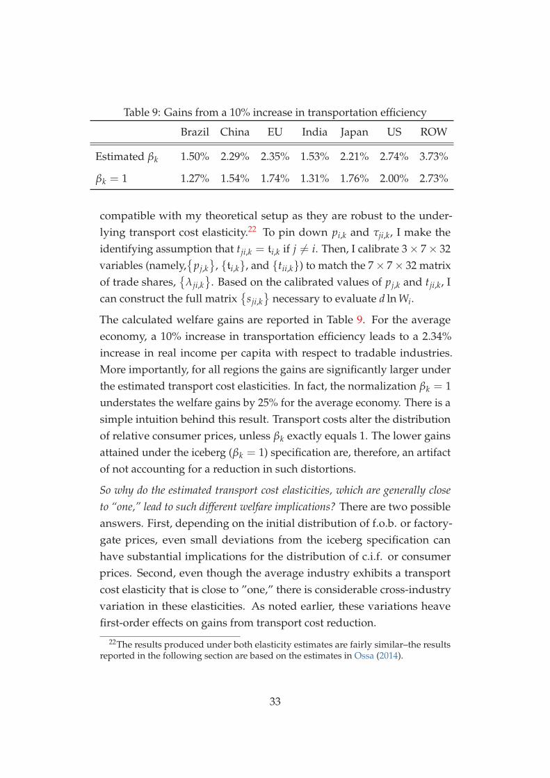
Table 9: Gains from a 10% increase in transportation efficiency

Brazil China EU India Japan US ROW

Estimated βk 1.50% 2.29% 2.35% 1.53% 2.21% 2.74% 3.73%

βk = 1 1.27% 1.54% 1.74% 1.31% 1.76% 2.00% 2.73%

compatible with my theoretical setup as they are robust to the under-lying transport cost elasticity.22 To pin down pi,k and τji,k, I make theidentifying assumption that tji,k = ti,k if j 6= i. Then, I calibrate 3× 7× 32variables (namely,

pj,k

, ti,k, and tii,k) to match the 7× 7× 32 matrixof trade shares,

λji,k

. Based on the calibrated values of pj,k and tji,k, I

can construct the full matrix

sji,k

necessary to evaluate d ln Wi.

The calculated welfare gains are reported in Table 9. For the averageeconomy, a 10% increase in transportation efficiency leads to a 2.34%increase in real income per capita with respect to tradable industries.More importantly, for all regions the gains are significantly larger underthe estimated transport cost elasticities. In fact, the normalization βk = 1understates the welfare gains by 25% for the average economy. There is asimple intuition behind this result. Transport costs alter the distributionof relative consumer prices, unless βk exactly equals 1. The lower gainsattained under the iceberg (βk = 1) specification are, therefore, an artifactof not accounting for a reduction in such distortions.

So why do the estimated transport cost elasticities, which are generally closeto “one,” lead to such different welfare implications? There are two possibleanswers. First, depending on the initial distribution of f.o.b. or factory-gate prices, even small deviations from the iceberg specification canhave substantial implications for the distribution of c.i.f. or consumerprices. Second, even though the average industry exhibits a transportcost elasticity that is close to ”one,” there is considerable cross-industryvariation in these elasticities. As noted earlier, these variations heavefirst-order effects on gains from transport cost reduction.

22The results produced under both elasticity estimates are fairly similar–the resultsreported in the following section are based on the estimates in Ossa (2014).

33

5 Conclusion

For the last decade, quantitative trade theory has taken remarkable stridesin determining the welfare consequence of globalization. With all theirmerit, however, existing theories of international trade rely on strongparametric assumptions. Most notably, the constant elasticity of substi-tution (CES) and the multiplicative trade cost assumptions. The pastfew years have seen a wave of new papers attempting to relax theseparametric restrictions. A prominent example is Adao et al. (2017) whoanalyze the consequences of the CES assumption. This paper contributesto this new wave, by highlighting the consequences and limitations ofthe multiplicative transport cost assumption.

The implications of the paper, however, span beyond basic welfare anal-ysis. The finding that physical weight is not an appropriate proxy forquantity has sharp implications for the empirical trade literature. In atradition that dates back to Moneta (1959), many studies on quality spe-cialization use value-to-weight ratios as a proxy for price or quality levels.Against the backdrop of this tradition, this paper highlights the weakrelationship between the value-to-weight ratio and unit price. This resultopens up an important avenue for future research. Namely, analyzing therobustness of existing findings to the distinction between value-to-weightand price or quality levels.

At broader level, my estimation of industry-level transport cost elasticitieshas basic implications for economic development and industrial policy.In view of the Alchian and Allen (1964) conjecture, high-quality exportsare less impeded by distance in industries featuring lower transportcost elasticities. As a result, high-quality suppliers have a comparativeadvantage in low-transport cost elasticity industries. This observationhas the potential to explain existing patterns of vertical specializationand North-South trade. Furthermore, it has immediate implications forindustrial policies targeted at quality-upgrading.

The implications of my analysis for optimal trade policy are more nu-anced. Beshkar and Lashkaripour (2017) demonstrate that non-linearitiesin production and delivery costs are an important source of variation

34

in optimal sectoral tariffs. The present paper highlights and estimatesa rather unexplored aspect of these non-linearities that stem from non-multiplicative transport costs. The elasticity estimates presented here can,thus, shed new light on the sectoral structure of optimal trade policy.

References

Abe, K. and J. S. Wilson (2009). Weathering the storm: investing in portinfrastructure to lower trade costs in east asia.

Adao, R., A. Costinot, and D. Donaldson (2017). Nonparametric coun-terfactual predictions in neoclassical models of international trade.American Economic Review 107(3), 633–89.

Alchian, A. A. and W. R. Allen (1964). University economics. Belmont,CA: Wadsworth Publishing Company.

Arkolakis, C., A. Costinot, and A. Rodriguez (2012). New trade models,same old gains. American Economic Review 102(1), 94.

Atkin, D. and D. Donaldson (2015). Who’s getting globalized? the size andimplications of intra-national trade costs. Technical report, NationalBureau of Economic Research.

Baldwin, R. and J. Harrigan (2011). Zeros, quality, and space: Trade theoryand trade evidence. American Economic Journal: Microeconomics 3(2),60–88.

Beshkar, M. and A. Lashkaripour (2017). Interdependence of trade policiesin general equilibrium.

Blonigen, B. A. and W. W. Wilson (2008). Port efficiency and trade flows.Review of International Economics 16(1), 21–36.

Caliendo, L. and F. Parro (2015). Estimates of the trade and welfare effectsof nafta. The Review of Economic Studies 82(1), 1–44.

35

Clark, X., D. Dollar, and A. Micco (2004). Port efficiency, maritime trans-port costs, and bilateral trade. Journal of development economics 75(2),417–450.

Cosar, K. and B. Demir (2017). Shipping inside the box: Containerizationand trade.

Costinot, A. and A. Rodríguez-Clare (2013). Trade theory with num-bers: Quantifying the consequences of globalization. Technical report,National Bureau of Economic Research.

Crozet, M., K. Head, and T. Mayer (2012). Quality sorting and trade: Firm-level evidence for french wine. The Review of Economic Studies 79(2),609–644.

Dekle, R., J. Eaton, and S. Kortum (2007). Unbalanced trade. Technicalreport, National Bureau of Economic Research.

Donaldson, D. (2018). Railroads of the raj: Estimating the impact oftransportation infrastructure. American Economic Review 108(4-5), 899–934.

Donaldson, D. and R. Hornbeck (2016). Railroads and american eco-nomic growth: A “market access” approach. The Quarterly Journal ofEconomics 131(2), 799–858.

Eaton, J., M. Eslava, M. Kugler, and J. Tybout (2010). A search and learningmodel of export dynamics.(penn state university, unpublished).

Graaff, J. d. V. (1949). On optimum tariff structures. The Review of EconomicStudies, 47–59.

Hertel, T., D. Hummels, M. Ivanic, and R. Keeney (2007). How confidentcan we be of cge-based assessments of free trade agreements? EconomicModelling 24(4), 611–635.

Hummels, D., V. Lugovskyy, and A. Skiba (2009). The trade reducingeffects of market power in international shipping. Journal of DevelopmentEconomics 89(1), 84–97.

36

Hummels, D. and A. Skiba (2004). Shipping the good apples out? anempirical confirmation of the alchian-allen conjecture. Journal of PoliticalEconomy 112(6).

Irarrazabal, A., A. Moxnes, and L. D. Opromolla (2014). The tip of theiceberg: A quantitative framework for estimating trade costs. Review ofEconomics and Statistics (forthcoming).

Johnson, H. G. (1953). Optimum tariffs and retaliation. The Review ofEconomic Studies 21(2), 142–153.

Kugler, M. and E. Verhoogen (2012). Prices, plant size, and productquality. The Review of Economic Studies 79(1), 307–339.

Lashkaripour, A. (2015). Beyond gravity: the composition of multilateraltrade flows. CAEPR Working Paper 2015-006.

Martin, J. (2012). Markups, quality, and transport costs. European EconomicReview 56(4), 777–791.

Melitz, M. (2003). The impact of trade on aggregate industry productivityand intra-industry reallocations. Econometrica 71(6), 1695–1725.

Melitz, M. J. and S. J. Redding (2015). New trade models, new welfareimplications. American Economic Review 105(3), 1105–46.

Moneta, C. (1959). The estimation of transportation costs in internationaltrade. The Journal of Political Economy, 41–58.

Ossa, R. (2014). Trade wars and trade talks with data. The AmericanEconomic Review 104(12), 4104–4146.

Schott, P. K. (2008, 01). The relative sophistication of chinese exports.Economic Policy 23, 5–49.

Simonovska, I. and M. E. Waugh (2014). Trade models, trade elastici-ties, and the gains from trade. Technical report, National Bureau ofEconomic Research.

Sørensen, A. (2014). Additive versus multiplicative trade costs and thegains from trade liberalizations. Canadian Journal of Economics.

37

A The US Sample: Data and Estimation

Data Description. I show that all the documented patterns hold equallyin the publicly-available US import data compiled by Schott (2008). TheUS import data reports the f.o.b. value, freight and insurance charge (bothin US dollars), the quantity of goods, and the gross weight of shipmentsaggregated at the HS10 level, across all firms exporting from a givencountry to a given district in the US in a given year (1989-2015).23 The USsample adopts a finer classification of units than the Colombia sample. Forexample, while pairs (“PR”) or dozen (“DOZ”) correspond to item-count,they are treated as distinct units of measurement. Combined, the entriesthat report a derivative of item-count, constitute more than 45% of USimports. For 4,575,197 observations, (i) a non-zero quantity is reportedin units of count (“N” and “NO”), (ii) imports are exclusively shippedby air and vessel (i.e., “gen_val_yr = ves_val_yr + air_val_yr”), and (iii)the total weight reported, is non-zero. For 3,485,198, of these observation,I also have matching data for per capita GDP and geo-distance to the USfrom the CEPII. I, therefore, restrict my analysis of US imports to these3,355,734 observations, which provide full information on total weight,value, freight charge, and quantity. Note that while the final samplesdo not exclude potential outliers, the estimation results presented in thefollowing sections are fairly robust to such exclusions.24

Estimating Equations. In the US sample observation s, ωht correspondsto aggregate export from country of origin s, to US district ω, in productcategory h, in year t. The weight-price relationship is estimated using thefollowing equation

ln wgts,ωht = α · ln ps,ωht + δωht + εs,ωht,

23Note that while the Colombia data reports insurance and freight charges separately,the US data lumps up freight, insurance, and other charges (excluding US import duties)into one reported variable.

24The estimation results presented in Sections 3.2-3.3 change by less than 2 decimalpoints when I drop (i) entries reporting a quantity less than 2, (ii) entries reportinga value below $2500, and (iii) entries with a unit price below or above the 95 and 5percentiles of their HS10-year category.

38

The above equation includes district-product-year fixed effects, and ex-ploits variation across exporting countries within a district-product-yearcell.

The transport cost elasticity is estimated using the following log-lineartransport cost function:

ln τs,ωht = β · ln ps,ωht + κ · ln Ss,ωht + δωht + εs,ωht

Parametrically, the above equation is identical to estimating equation–Equation “10”– in Hummels and Skiba (2004). Furthermore, in line withthe aforementioned study, the estimation includes product-year fixedeffects, controls for scale effects with the total weight of all shipmentsaggregated into entry s, ωht, and also includes bilateral distance (DISTs)and the GDP per capita of the origin country as additional controls Theonly distinction is that Hummels and Skiba (2004) assume a uniformunit weight, wgts,ωht = χht, within product-year cells. Based on thisassumption, they compute the unit price and transport cost by inferringimport quantity from weight: Qs,ωht =Ws,ωht/χωht (with the term χωht

being absorbed by the fixed effect). Knowing that unit weight is non-uniform within cell ωht, I instead use actual data on import quantity tocalculate the unit price and unit transport cost per observation. FollowingHummels and Skiba (2004), I instrument for unit price and total weightwith tariff rates plus lagged unit price and total weight levels.

B The Weight-Price Relationship: Examples

To dig deeper into the weight-price relationship, this appendix plots the re-lationship for two suspect HS10 categories: “HS8712000000” (bicycles andother cycles) plus “HS9102190000” (quartz, metal-base wrist watches).For both products I find a strong, positive relationship between unitweight and f.o.b. unit price (Figure 3). Finally, I look closer at an HS10category in which imports are sourced from well-know internationalproviders: “HS8703239000” (compact passenger vehicle with 1500-2500ccengine). For each provider, I plot the average unit weight of imports

39

against the average f.o.b. unit price (Figure 4). The results indicate thatluxury brands (Audi, Volvo, Jaguar) are systematically heavier than econ-omy brands (Daewoo, Skoda, Renault). The positive relationship persistseven across varieties sold by the same brand in category “HS8703239000”(Figure 5).

C The Weight-Price Relation in Export Data

Section 3.2 established a systematic relationship between the unit weightand unit price of imports. Here, I demonstrate that this relationshipextends to export data. To this end, I run the following regression on thetransaction-level Colombian export data:

ln wgts,ωiht = α · ln ps,ωiht + δωht + εs,ωiht

where observation s, ωiht corresponds to shipment s, exported by Colom-bian firm ω, to market i, in HS10 product h–year t. The fixed effect δωht

accounts for the determinants of unit weight that are invariant across ship-ments from firm ω in product category h, year t. The above specificationidentifies α based on across shipment variation within firm-product-yearcells. Alternatively, I run the above regression conditioning on product-destination-year fixed effects. Both specifications imply similar estimatesfor α ( first two columns in Table 10), and closely resemble the import-sideestimates. I also identify the weight-price relationship using product-levelUS export data. In particular, I identify α by exploiting across marketvariation in export unit prices and weights within HS10 product-yearcells. Again, the estimated elasticity (reported in the last column of Table10) closely resembles the import-side estimates.

40

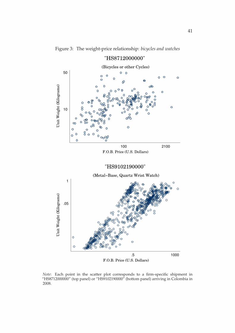
41

Figure 3: The weight-price relationship: bicycles and watches

10

50

Un

it W

eig

ht

(Kil

ogra

ms)

100 2100

F.O.B. Price (U.S. Dollars)

(Bicycles or other Cycles)

"HS8712000000"

.05

1

Un

it W

eig

ht

(Kil

ogra

ms)

.5 1000


(Metal−Base, Quartz Wrist Watch)

"HS9102190000"

Note: Each point in the scatter plot corresponds to a firm-specific shipment in“HS8712000000” (top panel) or “HS9102190000” (bottom panel) arriving in Colombia in2008.

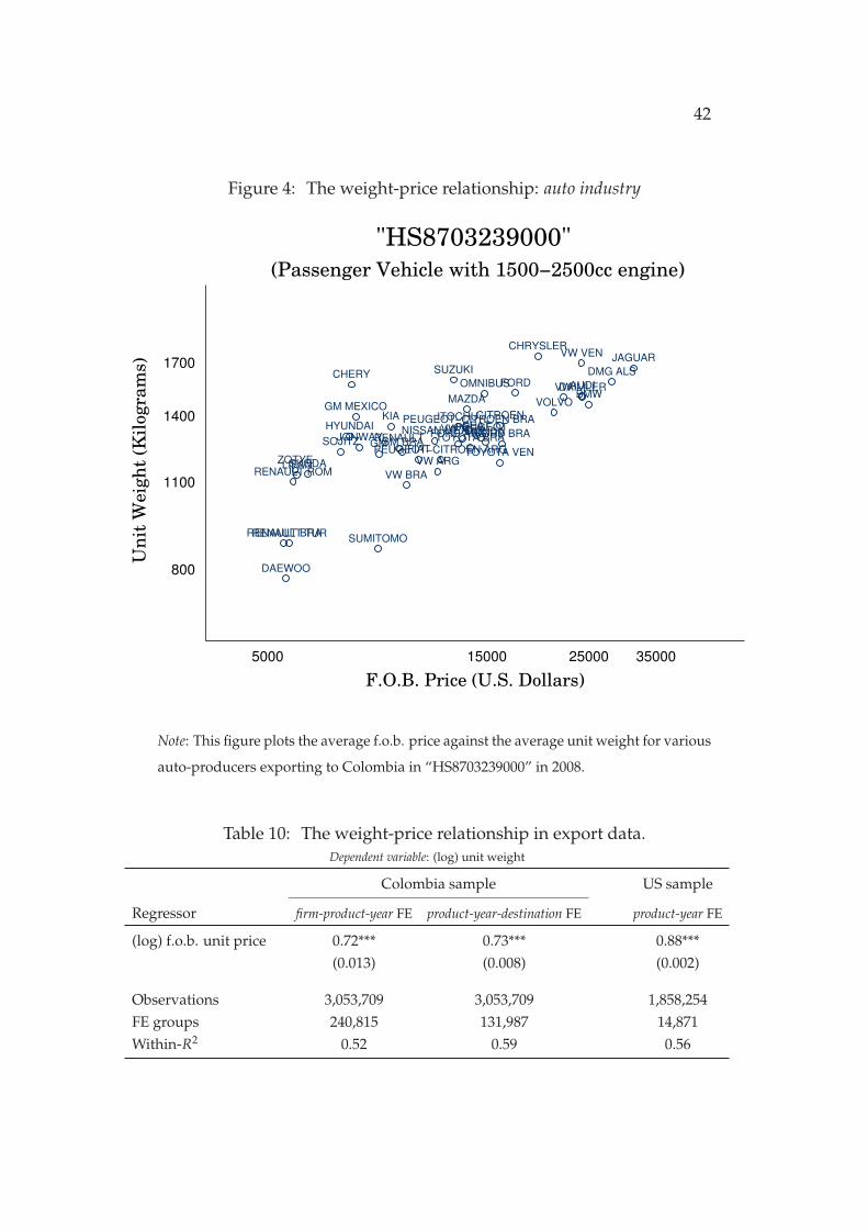
42

Figure 4: The weight-price relationship: auto industry

AUDIBMW

CHERY

CHRYSLER

CITROEN

DAEWOO

DAIMLER

DMG ALS

FIAT

FORD

FORD ARGFORD BRAGMGM BRA

GM MEXICO

HONDAHYUNDAI

ITOCHU

JAGUAR

JONWAY

KIA

LIFAN

MAZDA

NISSAN MEX

OMNIBUS

PEUGEOT

PEUGEOT−CITROEN ARG

PEUGEOT−CITROEN BRA

RENAULT

RENAULT BRA

RENAULT ROM

RENAULT TUR

SEAT

SKODA

SOJITZ

SUMITOMO

SUZUKI

TOYOTA BRA

TOYOTA VEN

VOLVO

VW

VW ARG

VW BRA

VW MEX

VW VEN

ZOTYE

800

1100

1400

1700

Un

it W

eig

ht

(Kil

ogra

ms)

5000 15000 25000 35000


(Passenger Vehicle with 1500−2500cc engine)

"HS8703239000"

Note: This figure plots the average f.o.b. price against the average unit weight for various

auto-producers exporting to Colombia in “HS8703239000” in 2008.

Table 10: The weight-price relationship in export data.Dependent variable: (log) unit weight


Regressor firm-product-year FE product-year-destination FE product-year FE

(log) f.o.b. unit price 0.72*** 0.73*** 0.88***(0.013) (0.008) (0.002)

Observations 3,053,709 3,053,709 1,858,254FE groups 240,815 131,987 14,871Within-R2 0.52 0.59 0.56

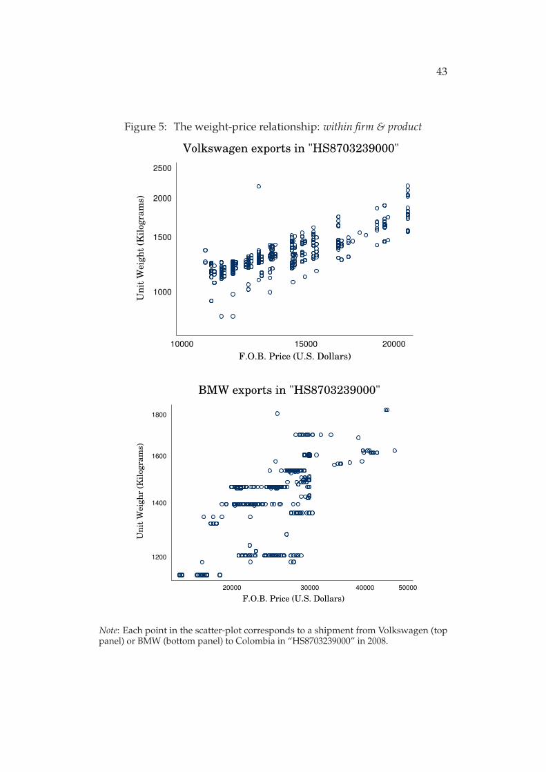
43

Figure 5: The weight-price relationship: within firm & product

1000

1500

2000

2500

Un

it W

eig

ht

(Kil

ogra

ms)

10000 15000 20000


Volkswagen exports in "HS8703239000"

1200

1400

1600

1800

Un

it W

eig

hr

(Kil

ogra

ms)

20000 30000 40000 50000


BMW exports in "HS8703239000"

Note: Each point in the scatter-plot corresponds to a shipment from Volkswagen (toppanel) or BMW (bottom panel) to Colombia in “HS8703239000” in 2008.

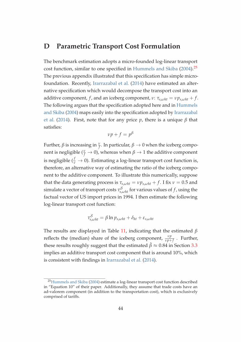
D Parametric Transport Cost Formulation

The benchmark estimation adopts a micro-founded log-linear transportcost function, similar to one specified in Hummels and Skiba (2004).25

The previous appendix illustrated that this specification has simple micro-foundation. Recently, Irarrazabal et al. (2014) have estimated an alter-native specification which would decompose the transport cost into anadditive component, f , and an iceberg component, ν: τs,ωht = νps,ωht + f .The following argues that the specification adopted here and in Hummelsand Skiba (2004) maps easily into the specification adopted by Irarrazabalet al. (2014). First, note that for any price p, there is a unique β thatsatisfies:

νp + f = pβ

Further, β is increasing in νf . In particular, β→ 0 when the iceberg compo-

nent is negligible ( νf → 0), whereas when β→ 1 the additive component

is negligible ( fν → 0). Estimating a log-linear transport cost function is,

therefore, an alternative way of estimating the ratio of the iceberg compo-nent to the additive component. To illustrate this numerically, supposethat the data generating process is τs,ωht = νps,ωht + f . I fix ν = 0.5 andsimulate a vector of transport costs τSs,ωht for various values of f , using thefactual vector of US import prices in 1994. I then estimate the followinglog-linear transport cost function:

τSs,ωht = β ln ps,ωht + δht + εs,ωht

The results are displayed in Table 11, indicating that the estimated β

reflects the (median) share of the iceberg component, νpνp+ f . Further,

these results roughly suggest that the estimated β ≈ 0.84 in Section 3.3implies an additive transport cost component that is around 10%, whichis consistent with findings in Irarrazabal et al. (2014).

25Hummels and Skiba (2004) estimate a log-linear transport cost function describedin “Equation 10” of their paper. Additionally, they assume that trade costs have anad-valorem component (in addition to the transportation cost), which is exclusivelycomprised of tariffs.

44

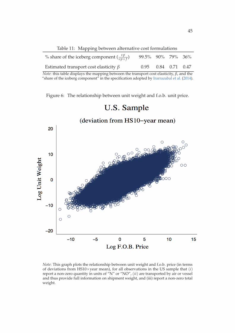
45

Table 11: Mapping between alternative cost formulations

% share of the iceberg component ( νpνp+ f ) 99.5% 90% 79% 36%

Estimated transport cost elasticity β 0.95 0.84 0.71 0.47Note: this table displays the mapping between the transport cost elasticity, β, and the“share of the iceberg component” in the specification adopted by Irarrazabal et al. (2014).

Figure 6: The relationship between unit weight and f.o.b. unit price.

Note: This graph plots the relationship between unit weight and f.o.b. price (in termsof deviations from HS10×year mean), for all observations in the US sample that (i)report a non-zero quantity in units of “N” or “NO”, (ii) are transported by air or vesseland thus provide full information on shipment weight, and (iii) report a non-zero totalweight.

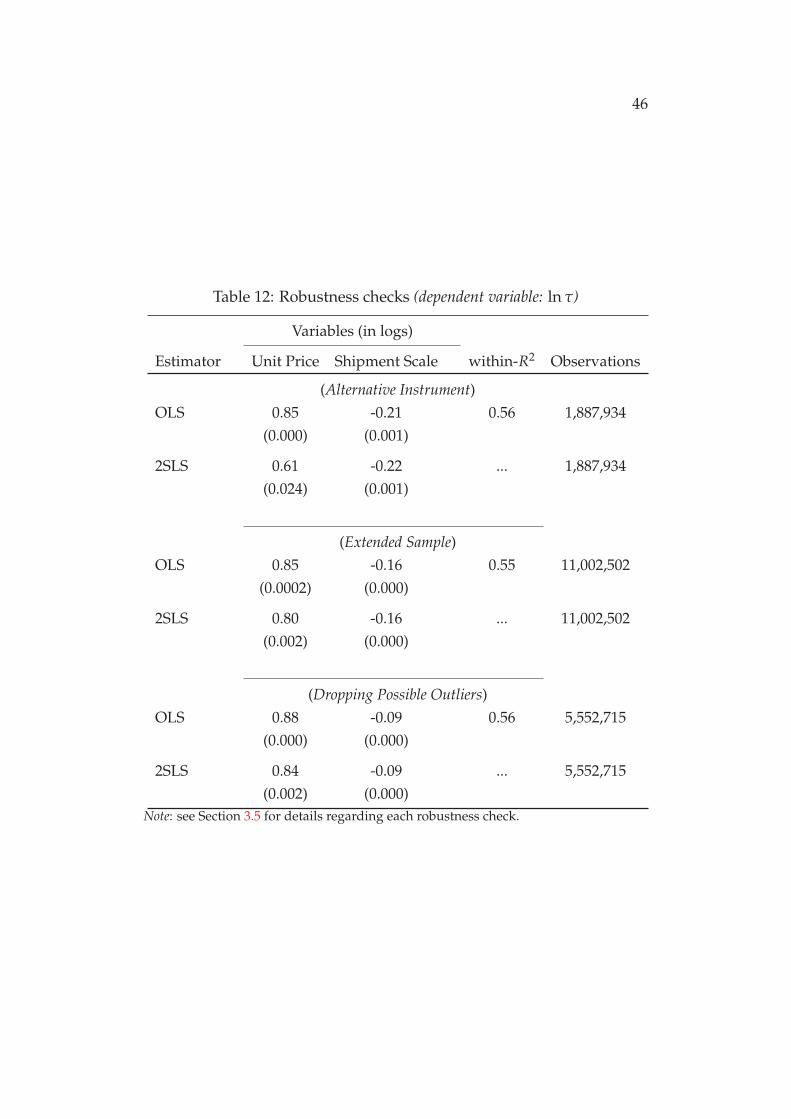
46

Table 12: Robustness checks (dependent variable: ln τ)

Variables (in logs)

Estimator Unit Price Shipment Scale within-R2 Observations

(Alternative Instrument)OLS 0.85 -0.21 0.56 1,887,934

(0.000) (0.001)

2SLS 0.61 -0.22 ... 1,887,934(0.024) (0.001)

(Extended Sample)OLS 0.85 -0.16 0.55 11,002,502

(0.0002) (0.000)

2SLS 0.80 -0.16 ... 11,002,502(0.002) (0.000)

(Dropping Possible Outliers)OLS 0.88 -0.09 0.56 5,552,715

(0.000) (0.000)

2SLS 0.84 -0.09 ... 5,552,715(0.002) (0.000)

Note: see Section 3.5 for details regarding each robustness check.

Estimating the International Transport Cost...

Documents

Transcript of Estimating the International Transport Cost...