1

2

3

0.0

0.1

0.2

0.3

0.4

0.5

0.6

0.7

0.8

0.9

1.0

1 10 100 1000 10000

Cum

ulat

ive

frac

tion

Particle size m

0

0.1

0.2

0.3

0.4

0.5

0.6

1 10 100 1000 10000

4

0.00

0.10

0.20

0.30

0.40

0.50

0.60

0.70

0.80

0.90

1.00

0.1 1 10 100 1000

F(x)

Particle size m

median 6.75 std 1.65

median 5.00 std 2.655

Mass recovery of solids in a dynamic separator such as gravity settling tank or sedimentation

centrifuge?

ET = G(x)dF0

1

5

0

0.1

0.2

0.3

0.4

0.5

0.6

0.7

0.8

0.9

0.01 0.1 1 10 100

dF(x

)/d(ln

(x))

Particle size m

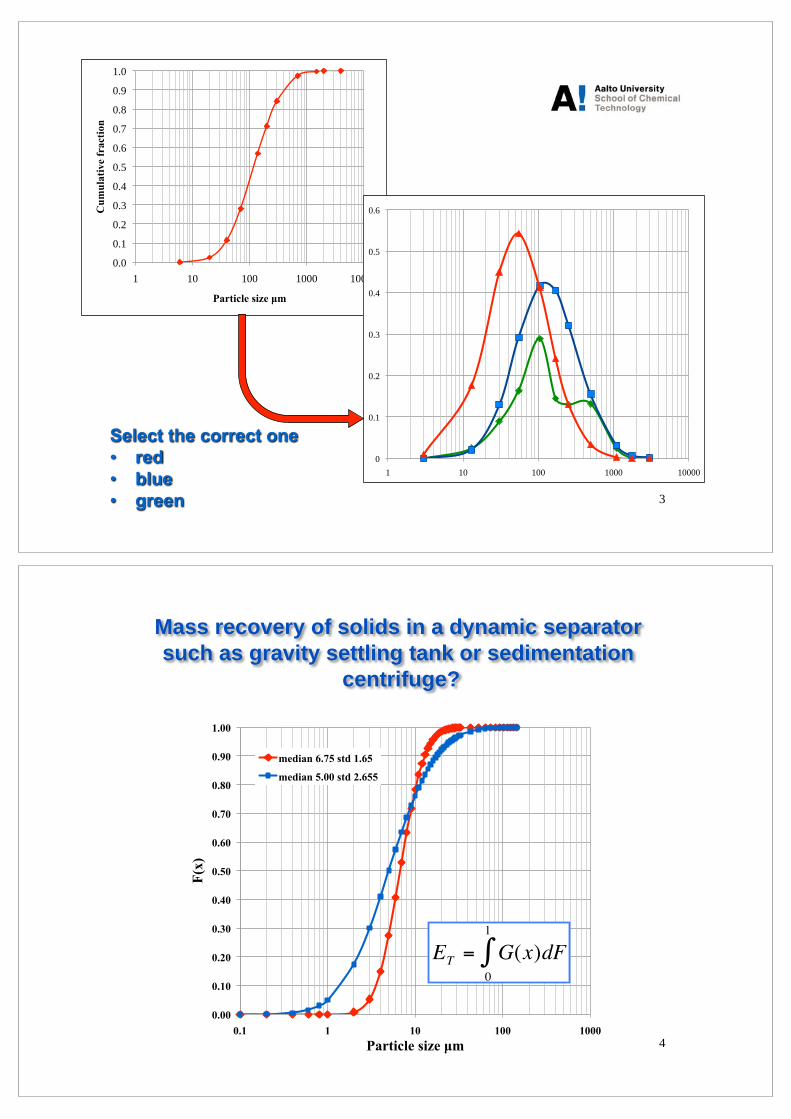
Median 6.75 std 1.65

Median 5.00 std 2.655

Mass recovery of solids in a dynamic separator ? Arithmetic mean diameter = 7.65 m for both distributions

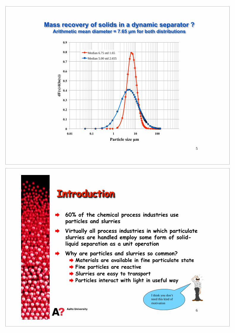
60% of the chemical process industries use particles and slurries

Virtually all process industries in which particulate slurries are handled employ some form of solid-liquid separation as a unit operation

Why are particles and slurries so common? Materials are available in fine particulate state Fine particles are reactive Slurries are easy to transport Particles interact with light in useful way

6

I think you dont need this kind of motivation

Particle size distribution directly affects the energy requirements of the processing steps and the characteristics of the final product.

In fact, the present lack of information on particle size distribution is a major cause of over grinding and low yield in the production of pigments, clays, and other materials made using slurries

7

Particle size is a critical parameter for a variety of operations in the chemical process industries

Accurate measurement of size is important because quality and performance of most particulate products are closely related to size distribution of fine particles

The past decade has seen rapid evolution and growth of applications for measuring size and shape

Particle Size, Shape, and Size Distribution

8

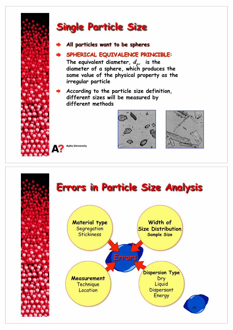
Single Particle Size

9

Material type Segregation Stickiness

Measurement Technique Location

Dispersion Type Dry

Liquid Dispersant

Energy

Width of Size Distribution

Sample Size

Errors in Particle Size Analysis

10

11

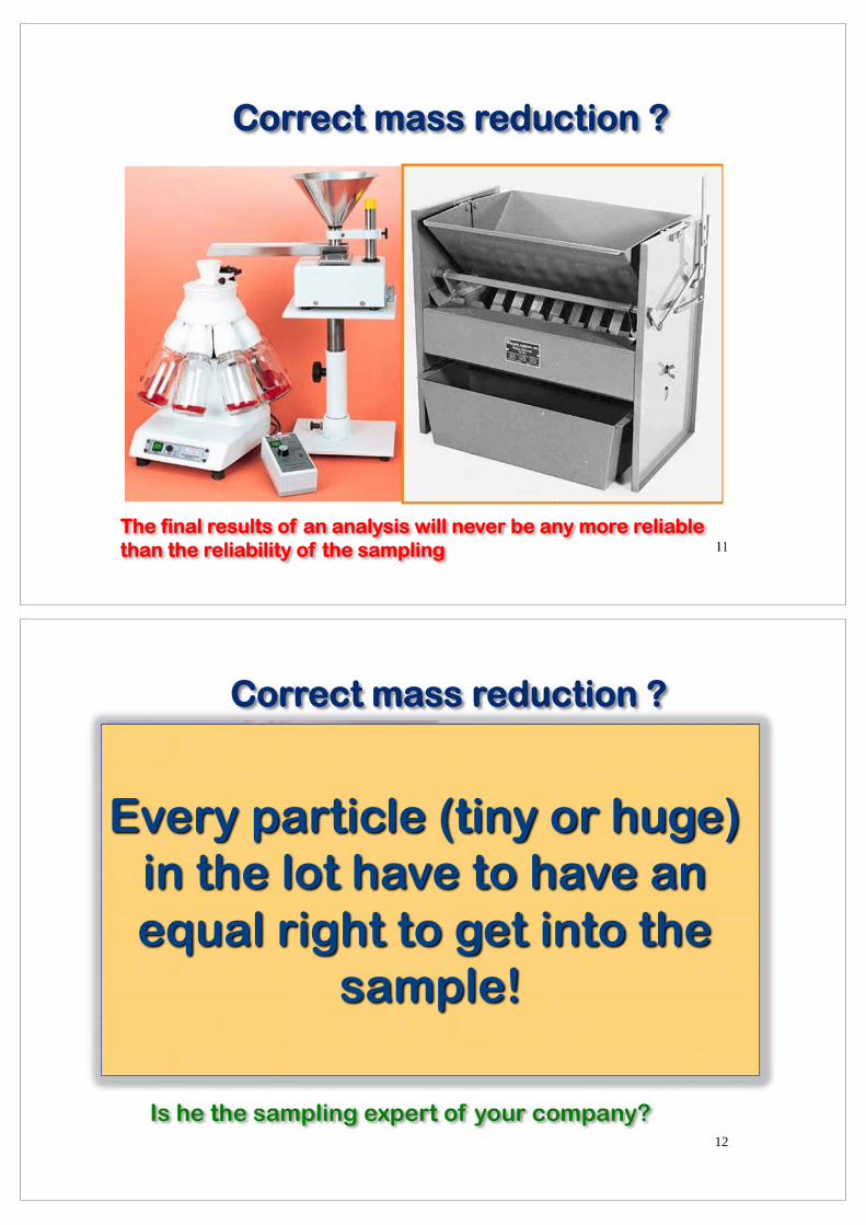
Correct mass reduction ?

The final results of an analysis will never be any more reliable than the reliability of the sampling

12

Correct mass reduction ?

Is he the sampling expert of your company?

Is he a better expert?

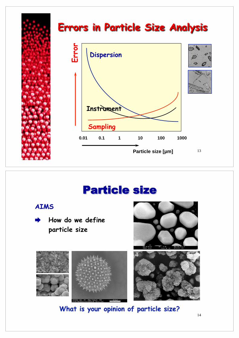
0.01 0.1 1 10 100 1000

Erro

r

Particle size [m]

Dispersion

Sampling

Instrument

Errors in Particle Size Analysis

13

Particle size AIMS

How do we define particle size

14

15

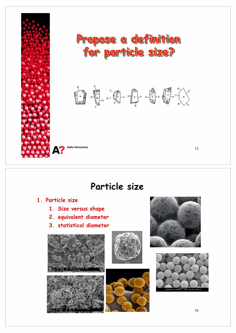
Particle size 1. Particle size

1. Size versus shape 2. equivalent diameter 3. statistical diameter

16

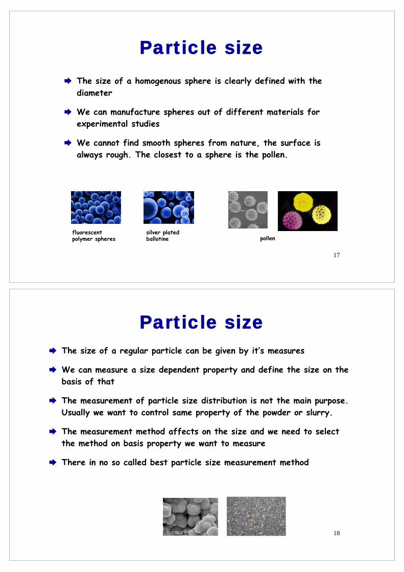
Particle size The size of a homogenous sphere is clearly defined with the diameter

We can manufacture spheres out of different materials for experimental studies

We cannot find smooth spheres from nature, the surface is always rough. The closest to a sphere is the pollen.

fluorescent polymer spheres

silver plated ballotine pollen

17

Particle size The size of a regular particle can be given by its measures

We can measure a size dependent property and define the size on the basis of that

The measurement of particle size distribution is not the main purpose. Usually we want to control same property of the powder or slurry.

The measurement method affects on the size and we need to select the method on basis property we want to measure

There in no so called best particle size measurement method

18

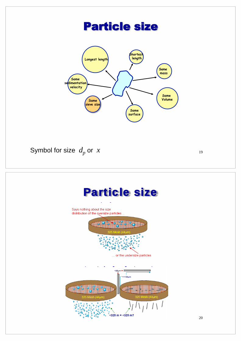
Particle size

Longest length Shortest

length

Same mass

Same Volume

Same surface

Same sieve size

Same sedimentation

velocity

Symbol for size dp or x 19

Particle size

20

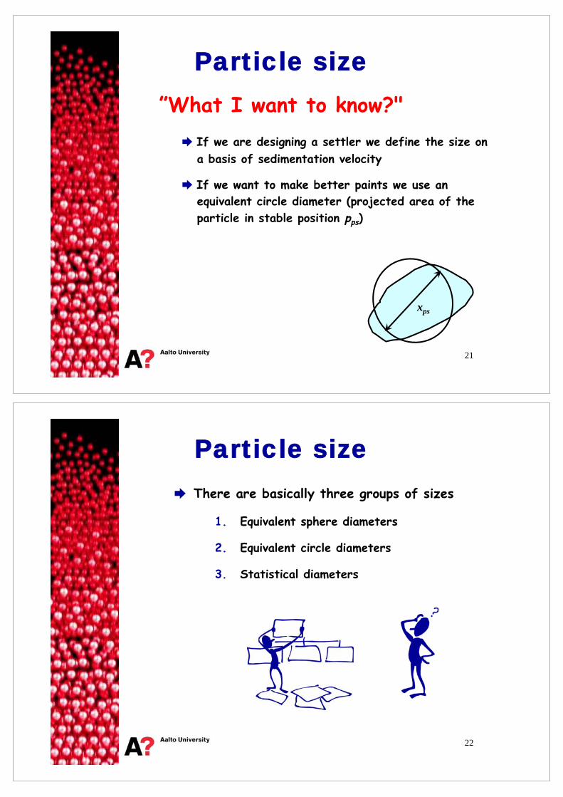
Particle size What I want to know?"

If we are designing a settler we define the size on a basis of sedimentation velocity

If we want to make better paints we use an equivalent circle diameter (projected area of the particle in stable position pps)

xps

21

Particle size There are basically three groups of sizes

1. Equivalent sphere diameters

2. Equivalent circle diameters

3. Statistical diameters

22

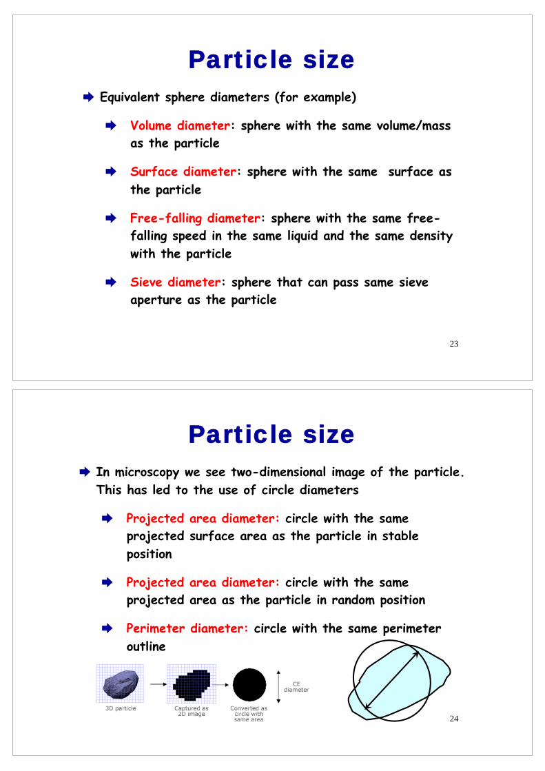
Particle size Equivalent sphere diameters (for example)

Volume diameter: sphere with the same volume/mass as the particle

Surface diameter: sphere with the same surface as the particle

Free-falling diameter: sphere with the same free-falling speed in the same liquid and the same density with the particle

Sieve diameter: sphere that can pass same sieve aperture as the particle

23

Particle size In microscopy we see two-dimensional image of the particle. This has led to the use of circle diameters

Projected area diameter: circle with the same projected surface area as the particle in stable position

Projected area diameter: circle with the same projected area as the particle in random position

Perimeter diameter: circle with the same perimeter outline

24

Particle size

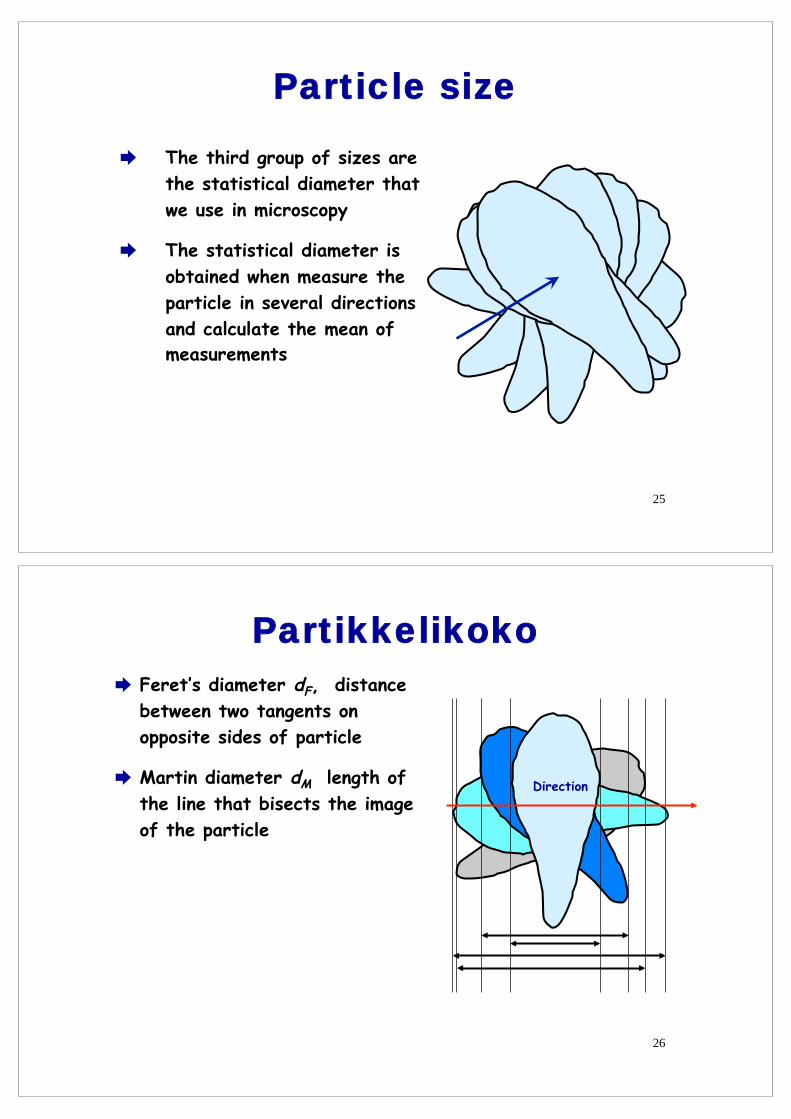
The third group of sizes are the statistical diameter that we use in microscopy

The statistical diameter is obtained when measure the particle in several directions and calculate the mean of measurements

25

Partikkelikoko Ferets diameter dF, distance between two tangents on opposite sides of particle

Martin diameter dM length of the line that bisects the image of the particle

Direction

26

Size distributions AIMS

Learn to interpret size distributions Learn to estimate the mean particle size Learn to select an appropriate theoretical size

distribution for modelling

27

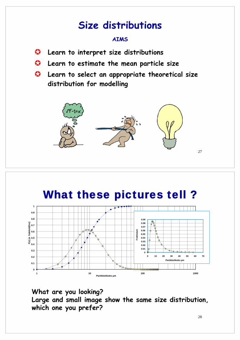
What these pictures tell ?

0

0.1

0.2

0.3

0.4

0.5

0.6

0.7

0.8

0.9

1

1 10 100 1000

F(x)

ja f

rakt

io/d

(lnx)

Partikkelikoko m

0 0.01 0.02 0.03 0.04 0.05 0.06 0.07 0.08 0.09

0 10 20 30 40 50 60 70

Frak

tio/

m

Partikkelikoko m

What are you looking? Large and small image show the same size distribution, which one you prefer?

28

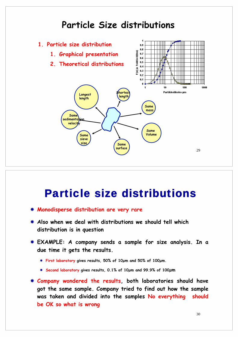
Particle Size distributions

1. Particle size distribution

1. Graphical presentation

2. Theoretical distributions

29

Longest length

Shortest length

Same mass

Same Volume

Same surface

Same sieve size

Same sedimentation

velocity

Particle size distributions Monodisperse distribution are very rare

Also when we deal with distributions we should tell which distribution is in question

EXAMPLE: A company sends a sample for size analysis. In a due time it gets the results.

First laboratory gives results, 50% of 10m and 50% of 100m.

Second laboratory gives results, 0.1% of 10m and 99.9% of 100m

Company wondered the results, both laboratories should have got the same sample. Company tried to find out how the sample was taken and divided into the samples No everything should be OK so what is wrong

30

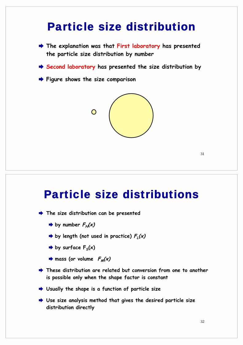
Particle size distribution The explanation was that First laboratory has presented the particle size distribution by number

Second laboratory has presented the size distribution by

Figure shows the size comparison

31

Particle size distributions The size distribution can be presented

by number FN(x)

by length (not used in practice) FL(x)

by surface FS(x)

mass (or volume FM(x)

These distribution are related but conversion from one to another is possible only when the shape factor is constant

Usually the shape is a function of particle size

Use size analysis method that gives the desired particle size distribution directly

32

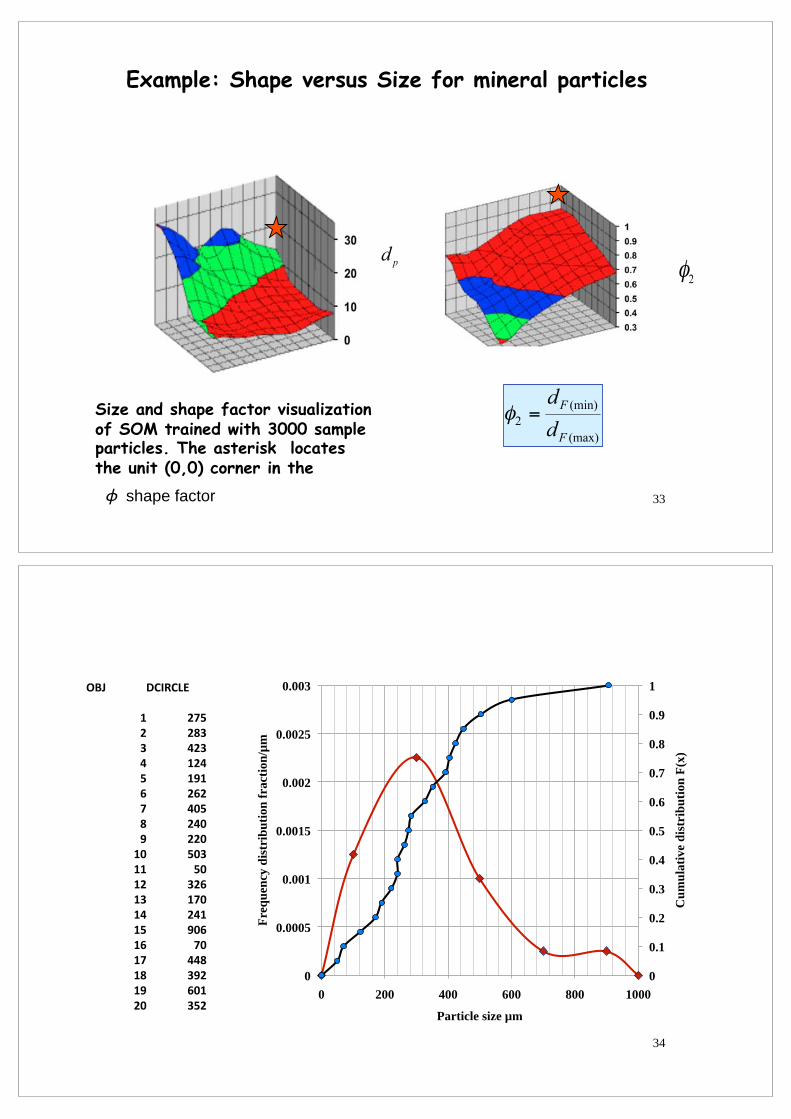
Size and shape factor visualization of SOM trained with 3000 sample particles. The asterisk locates the unit (0,0) corner in the

Example: Shape versus Size for mineral particles

shape factor 33

0

0.1

0.2

0.3

0.4

0.5

0.6

0.7

0.8

0.9

1

0

0.0005

0.001

0.0015

0.002

0.0025

0.003

0 200 400 600 800 1000

Particle size m

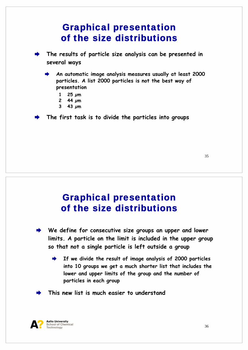
Cum

ulat

ive

dist

ribu

tion

F(x)

Freq

uenc

y di

stri

butio

n fr

actio

n/m

34

Graphical presentation of the size distributions

The results of particle size analysis can be presented in several ways

An automatic image analysis measures usually at least 2000 particles. A list 2000 particles is not the best way of presentation 1 25 m 2 44 m 3 43 m

The first task is to divide the particles into groups

35

We define for consecutive size groups an upper and lower limits. A particle on the limit is included in the upper group so that not a single particle is left outside a group

If we divide the result of image analysis of 2000 particles into 10 groups we get a much shorter list that includes the lower and upper limits of the group and the number of particles in each group

This new list is much easier to understand

36

Graphical presentation of the size distributions

Some methods give a grouped data. Sieve analysis is one of them

Lets us look for the data give in the table

37

Graphical presentation of the size distributions

sieve mass Fraction Fraction on the sieve passing

Sum

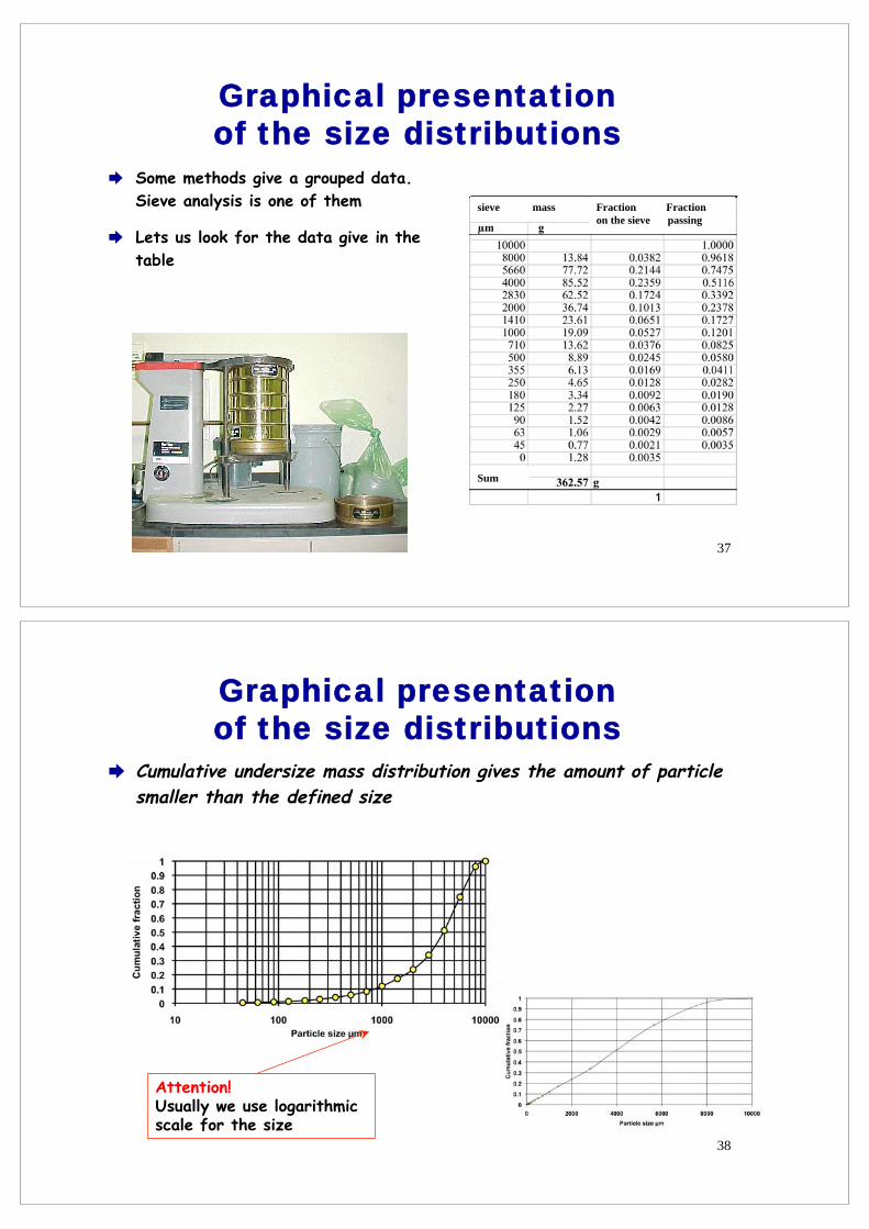
Cumulative undersize mass distribution gives the amount of particle smaller than the defined size

Attention! Usually we use logarithmic scale for the size

38

Graphical presentation of the size distributions

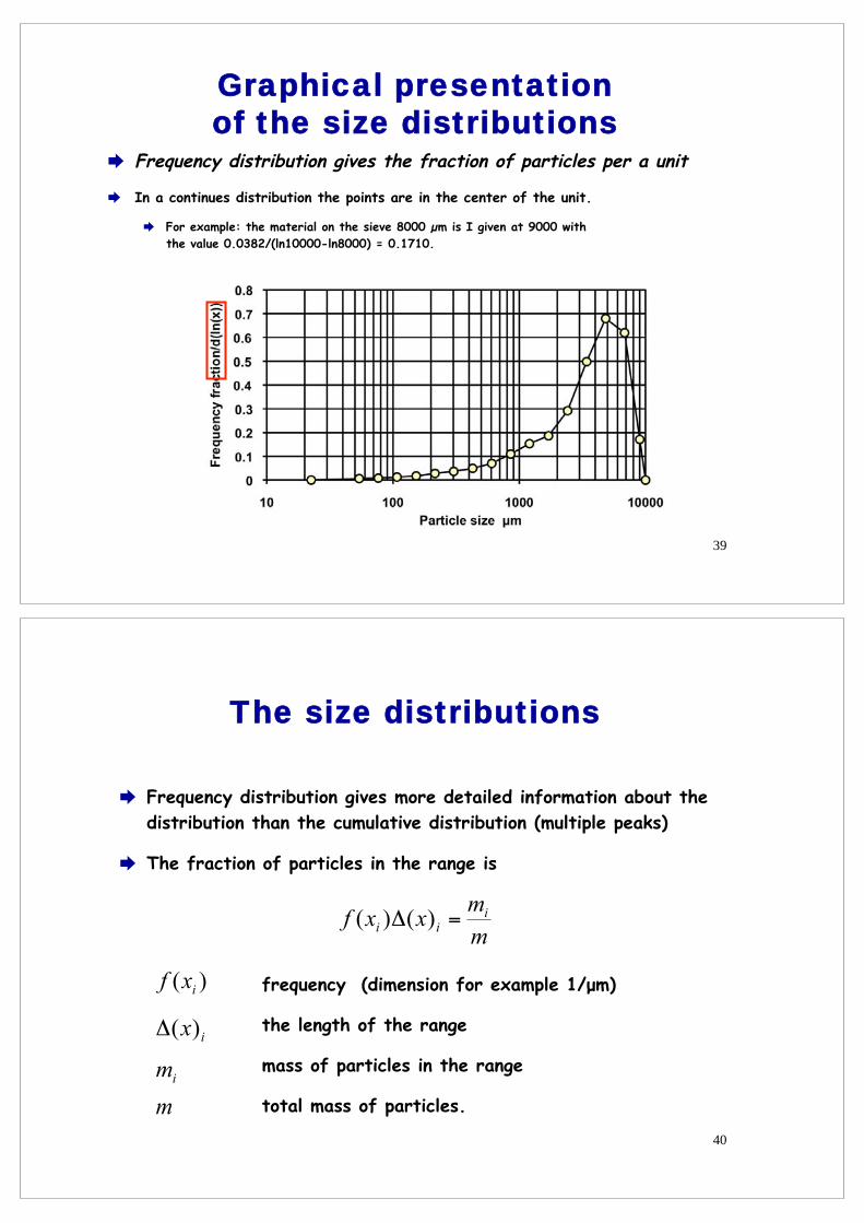
Frequency distribution gives the fraction of particles per a unit

In a continues distribution the points are in the center of the unit.

For example: the material on the sieve 8000 m is I given at 9000 with the value 0.0382/(ln10000-ln8000) = 0.1710.

39

Graphical presentation of the size distributions

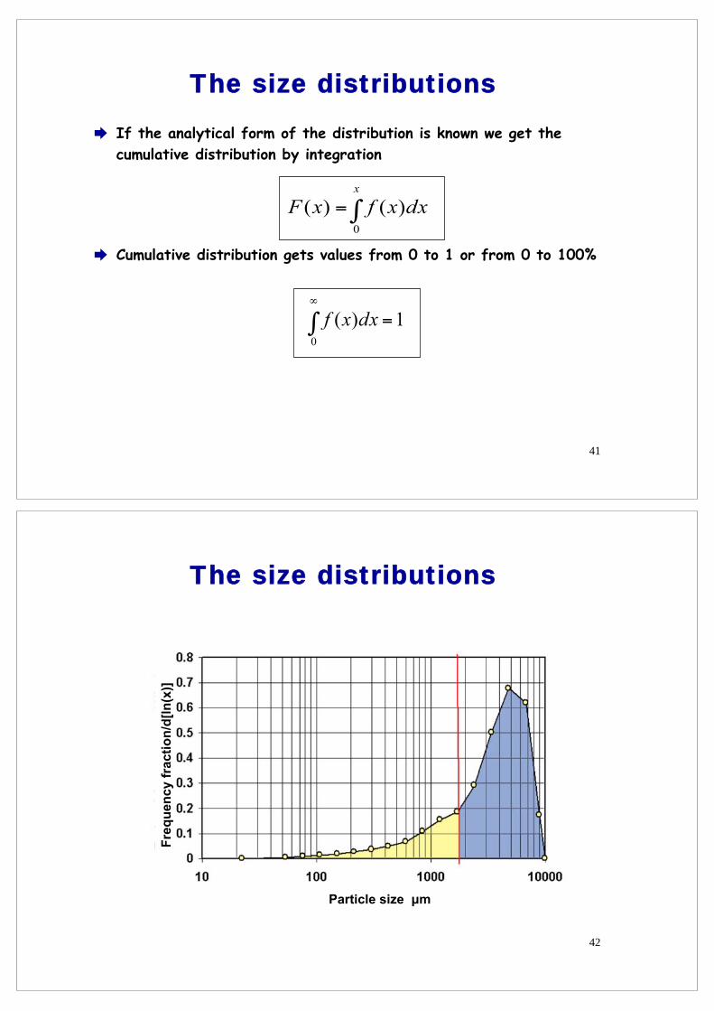
Frequency distribution gives more detailed information about the distribution than the cumulative distribution (multiple peaks)

The fraction of particles in the range is

frequency (dimension for example 1/m)

the length of the range

mass of particles in the range

total mass of particles.

40

The size distributions

If the analytical form of the distribution is known we get the cumulative distribution by integration

Cumulative distribution gets values from 0 to 1 or from 0 to 100%

41

The size distributions

42

The size distributions

Particle size m

Freq

uenc

y fr

actio

n/d[

ln(x

)]

Cumulative distribution can be presented as either using undersize or oversize presentation

Undersize distribution tells the amount of particles smaller than the defined size and oversize gives the amount of particles larger than the defined size

So that

Presentation of size distributions

F(x)oversize =1 F(x)undersize

43

Most measurement methods give the data in discrete form (sieve analysis)

Data can be presented as a histogram and plot then on it a rude approximation of a continuous frequency curve

However it is better to present first the cumulative distribution and draw a smooth curve through them.

If frequency distribution is required it can be calculated from

The size distributions

44

Earlier we agreed that the conversion from one distribution is possible only if the shape factor is constant

Les us assume that all particles are spheres

Types of particle size distributions

number distribution

length distribution (not used in practice )

surface distribution

mass distribution (volume distribution)

Conversion of the distributions

fA (x)

45

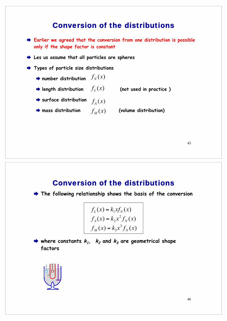
The following relationship shows the basis of the conversion

where constants k1, k2 and k3 are geometrical shape factors

46

Conversion of the distributions

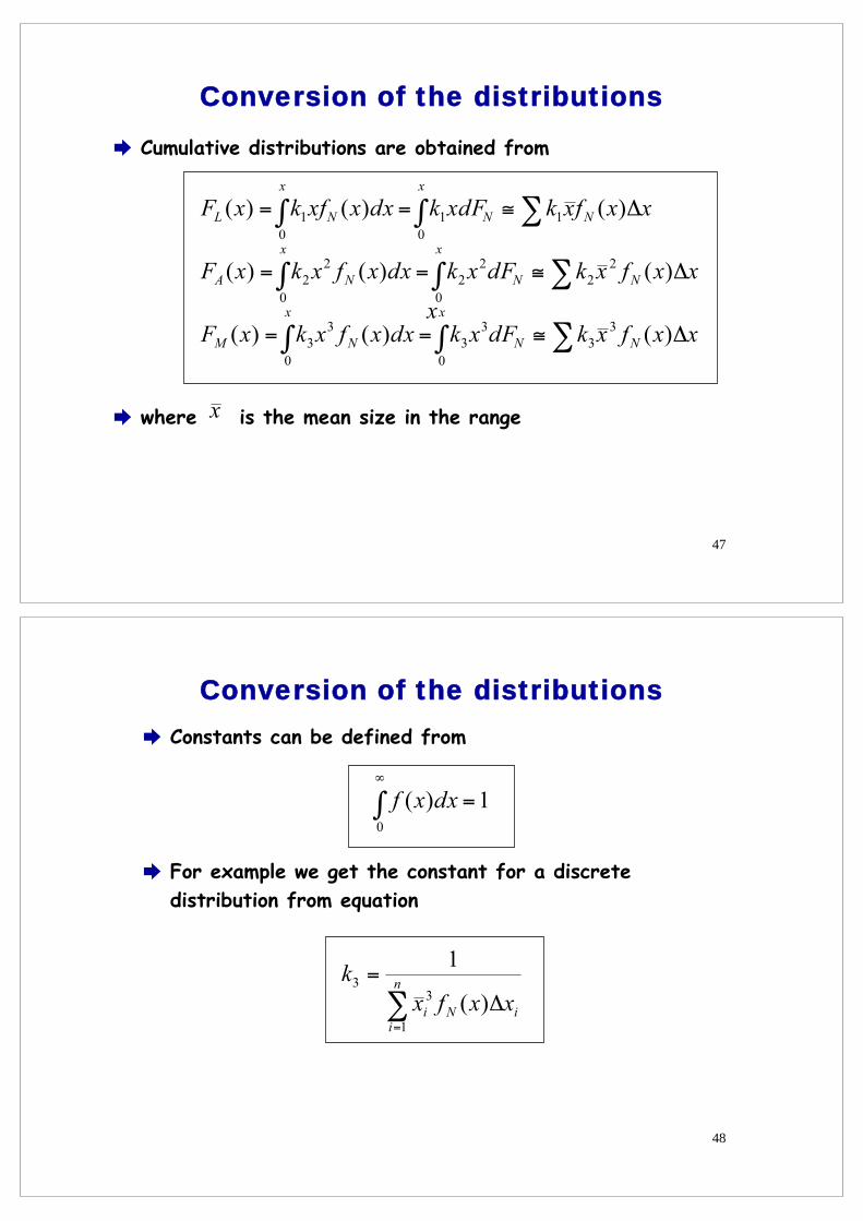
Cumulative distributions are obtained from

where is the mean size in the range

47

Conversion of the distributions

Constants can be defined from

For example we get the constant for a discrete distribution from equation

48

Conversion of the distributions

49

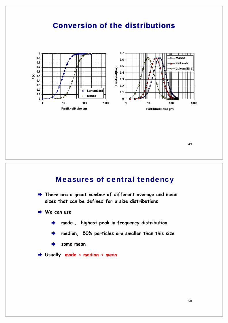
Conversion of the distributions

There are a great number of different average and mean sizes that can be defined for a size distributions

We can use

mode , highest peak in frequency distribution

median, 50% particles are smaller than this size

some mean

Usually mode < median < mean

Measures of central tendency

50

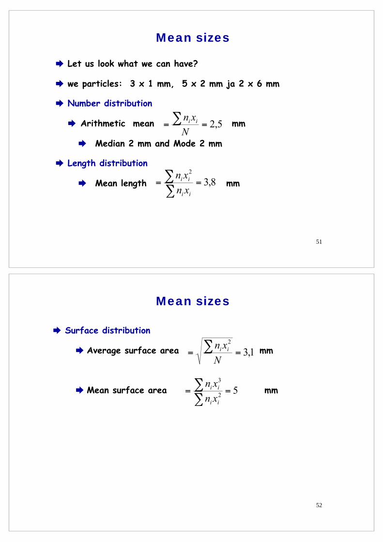
Let us look what we can have?

we particles: 3 x 1 mm, 5 x 2 mm ja 2 x 6 mm

Number distribution

Arithmetic mean mm

Median 2 mm and Mode 2 mm

Length distribution

Mean length mm

Mean sizes

51

Surface distribution

Average surface area mm

Mean surface area mm

Mean sizes

52

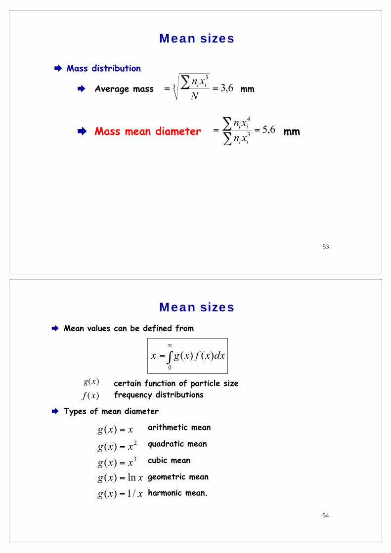
Mass distribution

Average mass mm

Mass mean diameter mm

Mean sizes

53

Mean values can be defined from

certain function of particle size frequency distributions

Types of mean diameter

arithmetic mean

quadratic mean

cubic mean

geometric mean

harmonic mean.

Mean sizes

g(x)

f (x)

54

When we use a mean we want it to describe the situation the best way

If you are not sure of the choice use arithmetic mean of the mass distribution

This is the best mean for separation processes, it describes the best the behaviour of the distribution in 9 cases out of 10

Mean sizes

x m =mixim

=nixi

4nixi

3= xi fM (xi)

i=1

N

xi

Remember this definition mi mass fraction in the range ni number fraction in the range 55

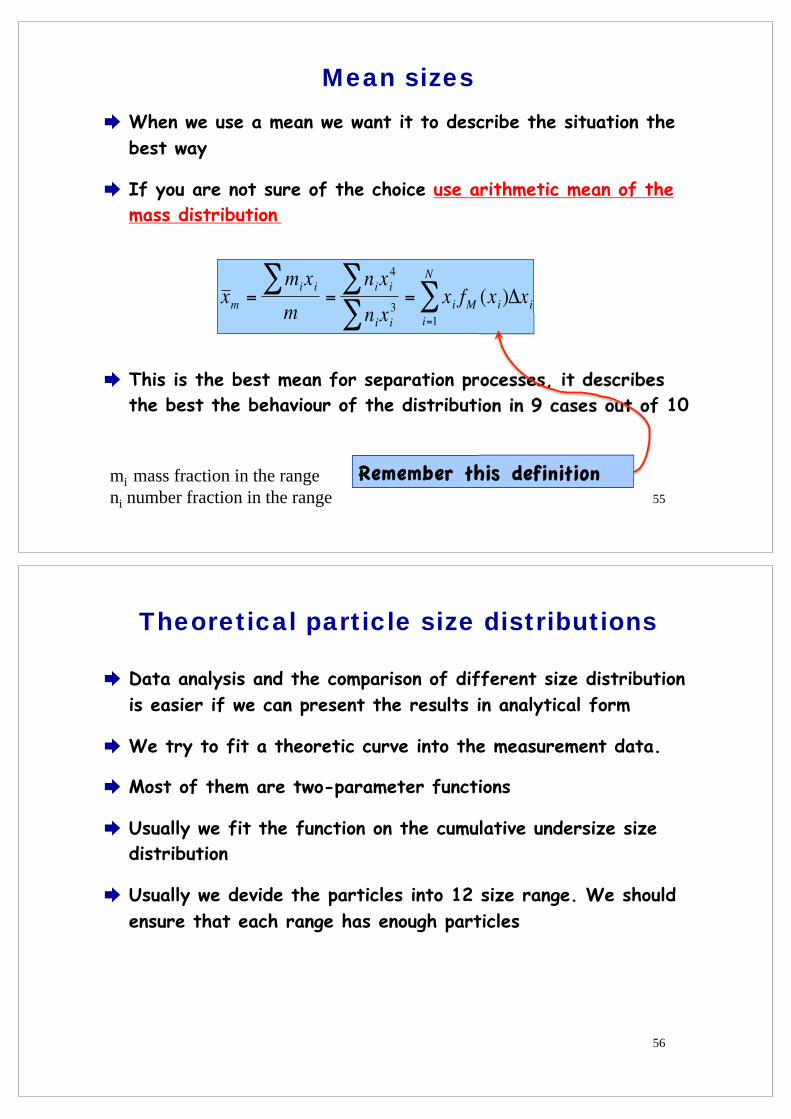
Data analysis and the comparison of different size distribution is easier if we can present the results in analytical form

We try to fit a theoretic curve into the measurement data.

Most of them are two-parameter functions

Usually we fit the function on the cumulative undersize size distribution

Usually we devide the particles into 12 size range. We should ensure that each range has enough particles

Theoretical particle size distributions

56

Log norm Exponential RR Weibull Arit norm

57

Theoretical particle size distributions

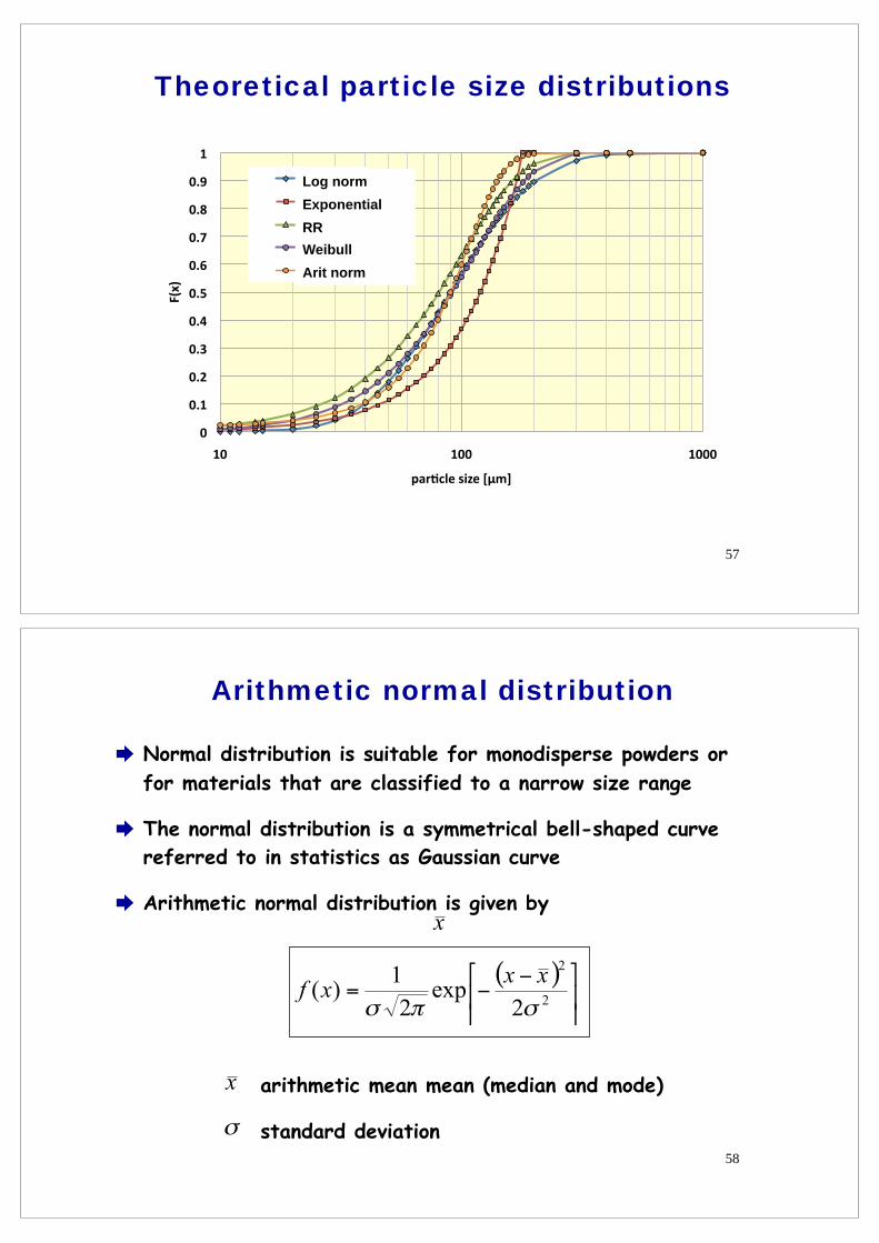
Normal distribution is suitable for monodisperse powders or for materials that are classified to a narrow size range

The normal distribution is a symmetrical bell-shaped curve referred to in statistics as Gaussian curve

Arithmetic normal distribution is given by

arithmetic mean mean (median and mode)

standard deviation

Arithmetic normal distribution

58

59

Arithmetic normal distribution

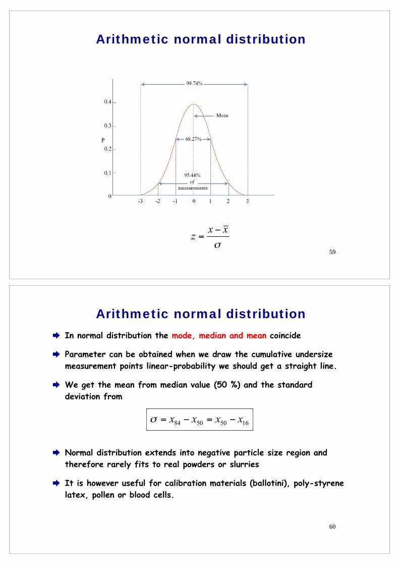
In normal distribution the mode, median and mean coincide

Parameter can be obtained when we draw the cumulative undersize measurement points linear-probability we should get a straight line.

We get the mean from median value (50 %) and the standard deviation from

Normal distribution extends into negative particle size region and therefore rarely fits to real powders or slurries

It is however useful for calibration materials (ballotini), poly-styrene latex, pollen or blood cells.

60

Arithmetic normal distribution

61

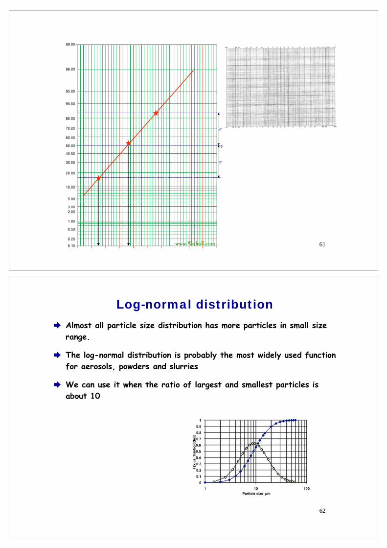
Almost all particle size distribution has more particles in small size range.

The log-normal distribution is probably the most widely used function for aerosols, powders and slurries

We can use it when the ratio of largest and smallest particles is about 10

Log-normal distribution

62

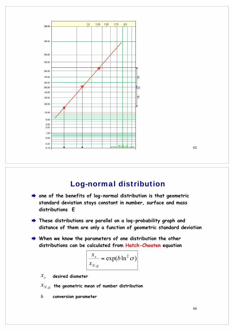
Log-normal size distribution is given by

geometric mean

geometric standard deviation.

The parameters are obtained when we draw cumulative undersize results on log-probability paper we should get a straight line

f (x) =1

x lng 2exp

ln x ln xg( )2

2ln2

63

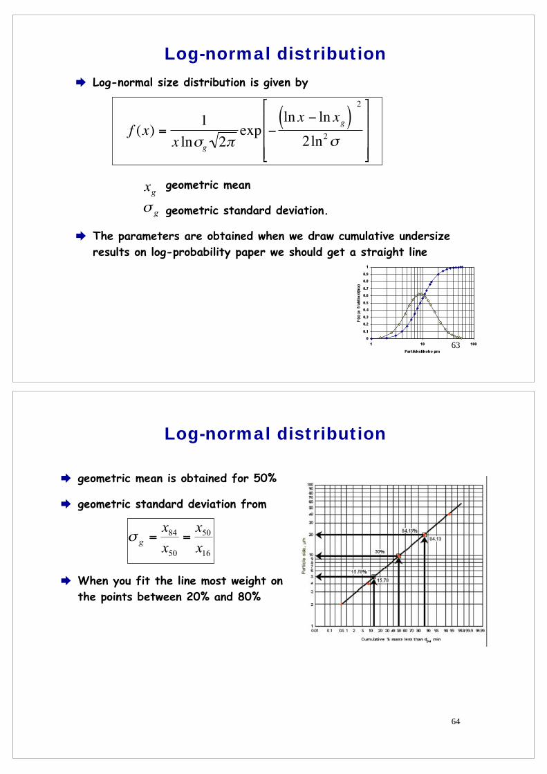
Log-normal distribution

geometric mean is obtained for 50%

geometric standard deviation from

When you fit the line most weight on the points between 20% and 80%

64

Log-normal distribution

65

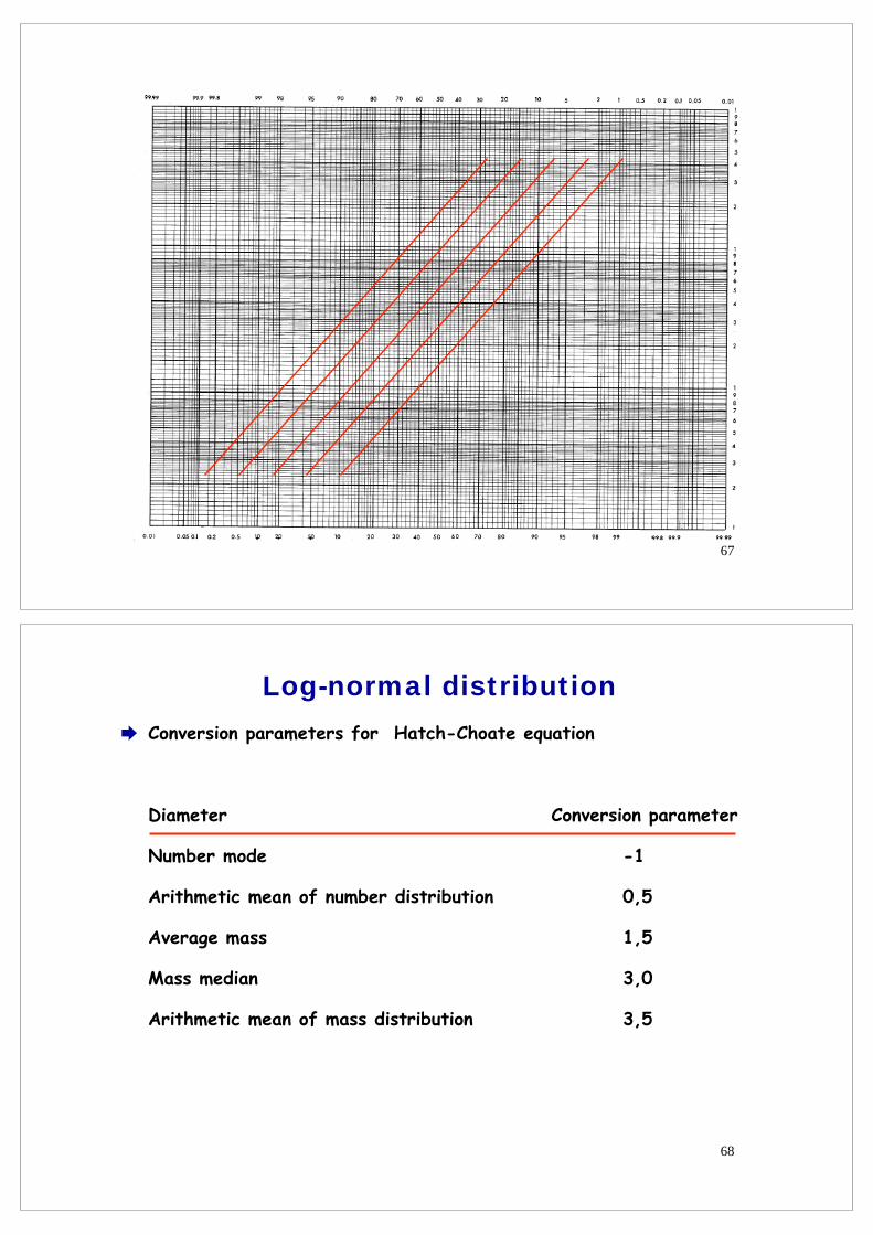
one of the benefits of log-normal distribution is that geometric standard deviation stays constant in number, surface and mass distributions E

These distributions are parallel on a loq-probability graph and distance of them are only a function of geometric standard deviation

When we know the parameters of one distribution the other distributions can be calculated from Hatch-Choaten equation

desired diameter

the geometric mean of number distribution

b conversion parameter

66

Log-normal distribution

67

Conversion parameters for Hatch-Choate equation

Diameter Conversion parameter

Number mode -1

Arithmetic mean of number distribution 0,5

Average mass 1,5

Mass median 3,0

Arithmetic mean of mass distribution 3,5

68

Log-normal distribution

69

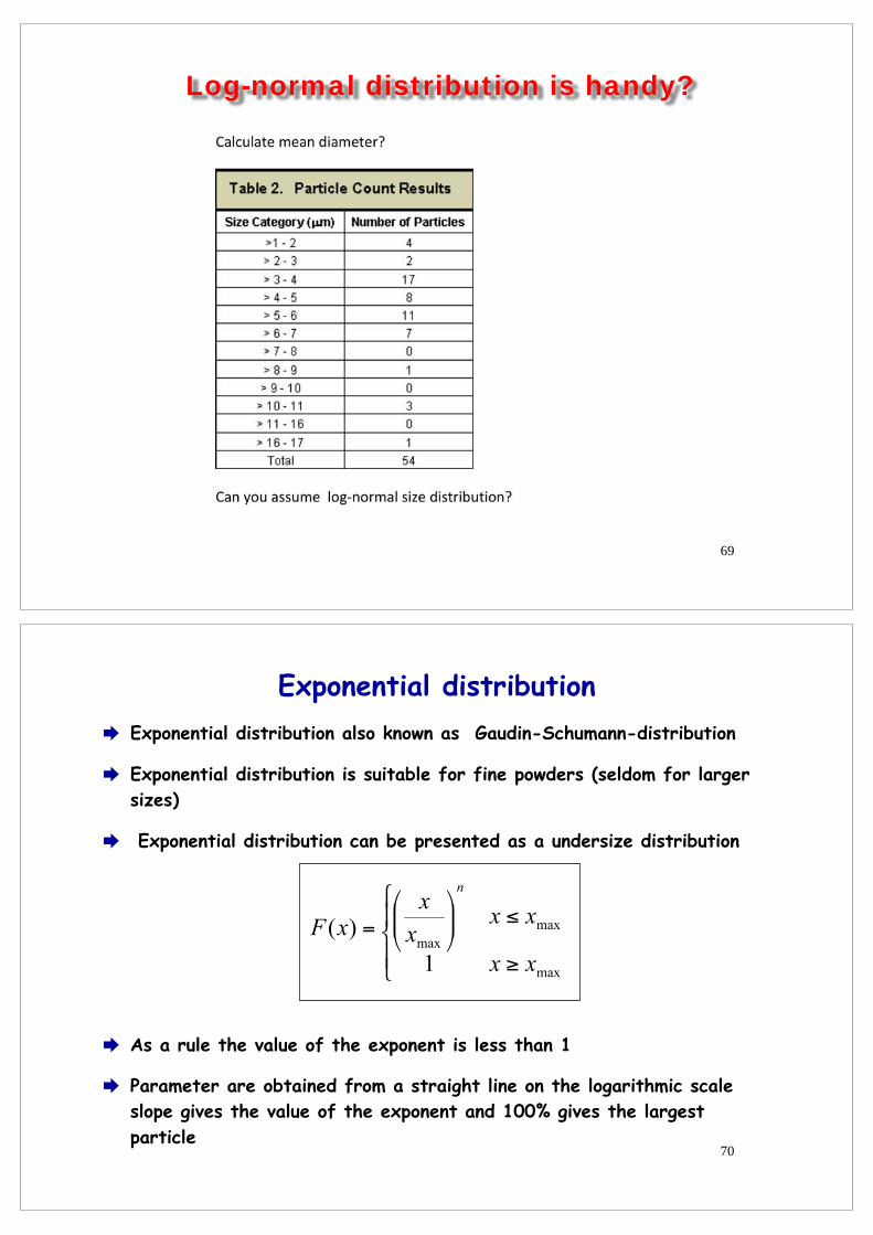
Log-normal distribution is handy?

Exponential distribution Exponential distribution also known as Gaudin-Schumann-distribution

Exponential distribution is suitable for fine powders (seldom for larger sizes)

Exponential distribution can be presented as a undersize distribution

As a rule the value of the exponent is less than 1

Parameter are obtained from a straight line on the logarithmic scale slope gives the value of the exponent and 100% gives the largest particle

70

Rosin-Rammler distribution Rosin-Rammler distribution is common in grinding it is also used for airborne dust liquid aerosols

Rosin-Rammler undersize distribution is given by

n is the exponential that defines the steepness of the cumulative curve and xR diameter so that 36,8 % of particles are larger than xR

If the value n is high the size distribution is narrow

This distribution is usually used for mass distribution

For example for screening results

71

Example

Sieve analysis results from a grinding mill

56,3 p-% < 75 m

22,0 p-% 75 - 105 m

0,2 p-% >150 m

Calculate the arithmetic mean. Assume that results follow the Rosin-Rammler distribution

Rosin-Rammler distribution

72

Write Rosin-Rammler equation in form

we get the parameters from the straight line

Rosin-Rammler distribution

73

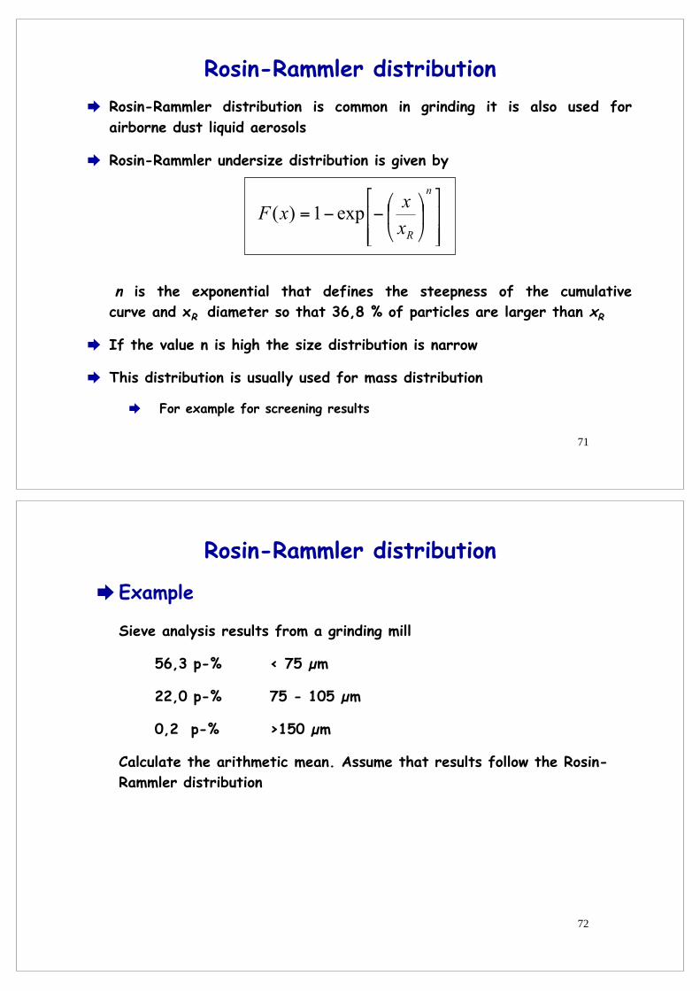
Calculate F(x) and make a table:

x F(x) ln x ln{ln[1/(1-F(x))]}

75 m 0,563 4,32 -0,19

105 m 0,783 4,65 0,42

150 m 0,998 5,01 0,83

ln xR = 4,42 xR = 83 m

the slope gives the value for n=3

74

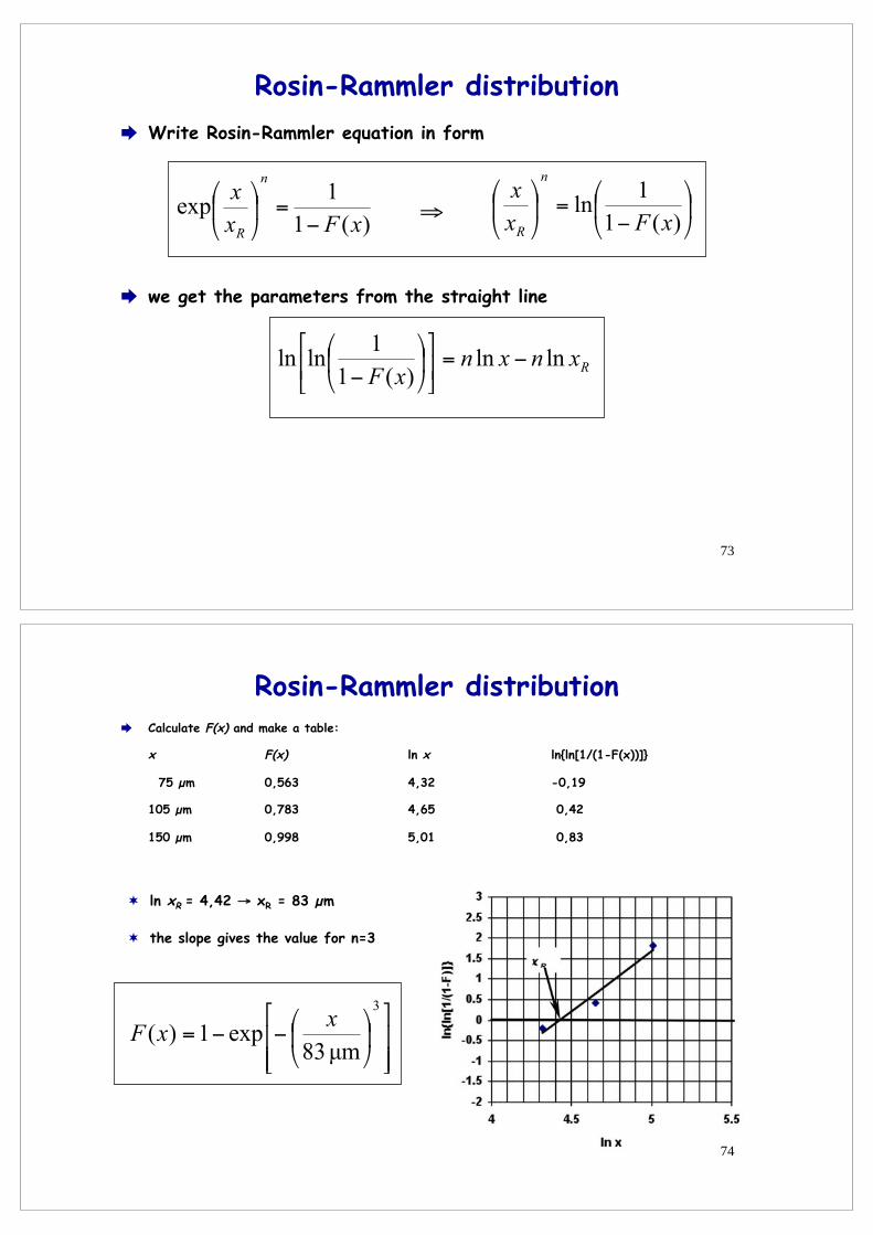
Rosin-Rammler distribution

Koko F(x) xi D[F(x)] xi*D[F(x)] 0 0.0000 5 0.0017 0.0087 10 0.0017 15 0.0121 0.1822 20 0.0139 25 0.0322 0.8057 30 0.0461 35 0.0598 2.0920 40 0.1059 45 0.0905 4.0713 50 0.1964 55 0.1182 6.5032 60 0.3146 65 0.1365 8.8733 70 0.4511 75 0.1405 10.5339 80 0.5916 85 0.1290 10.9636 90 0.7206 95 0.1055 10.0206 100 0.8260 105 0.0765 8.0276 110 0.9025 115 0.0488 5.6134 120 0.9513 125 0.0273 3.4069 130 0.9786 135 0.0132 1.7827 140 0.9918 145 0.0055 0.7983 150 0.9973 155 0.0020 0.3035 160 0.9992 165 0.0006 0.0972 170 0.9998 Mean size 74.0842 m 75

76

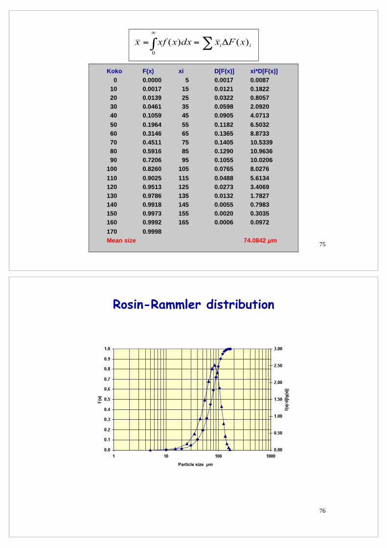
Rosin-Rammler distribution

Particle size m

Weibull distribution This distribution was originally derived for fragmentation of material under stress

Weibull distribution is a three parameter theoretical distribution

xu smallest size x0 characteristic size and m exponent

If distribution begins from zero it is same as Rosin-Rammler distribution

The main difficulty in using this distribution is to find the smallest size

77

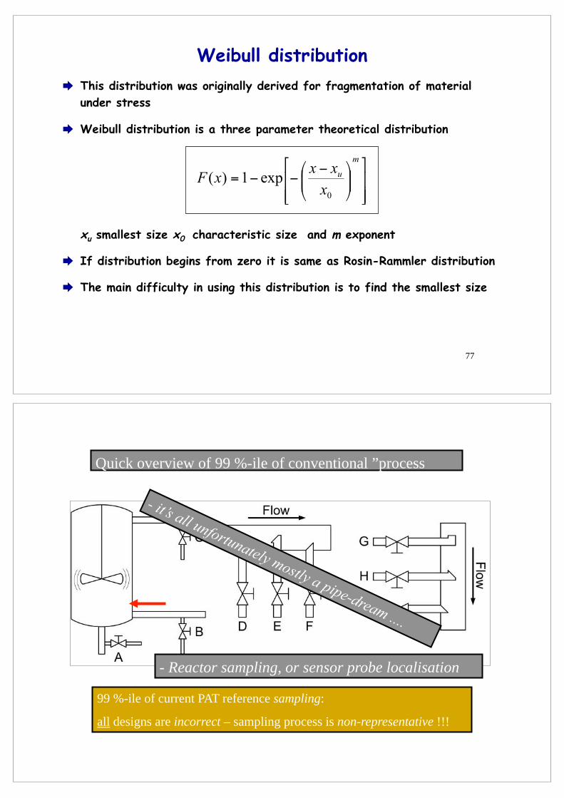
Quick overview of 99 %-ile of conventional process sampling design

99 %-ile of current PAT reference sampling:

all designs are incorrect sampling process is non-representative !!!

- Reactor sampling, or sensor probe localisation

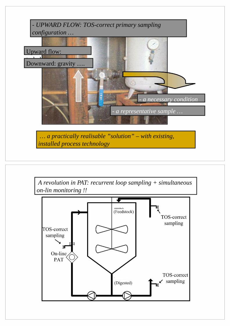
- UPWARD FLOW: TOS-correct primary sampling configuration

- a necessary condition for:

- a representative sample

a practically realisable solution with existing, installed process technology

Upward flow: turbulence . Downward: gravity .

A revolution in PAT: recurrent loop sampling + simultaneous on-lin monitoring !!