Mathematical Statistics, Lecture 6 Sufficiency · 2020-01-03 · Suﬃciency Given T (X ) = t, the...

Sufficiency

Sufficiency

MIT 18.655

Dr. Kempthorne

Spring 2016

1 MIT 18.655 Sufficiency

Sufficiency

Sufficiency

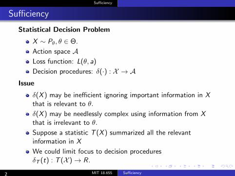
Statistical Decision Problem

X ∼ Pθ, θ ∈ Θ.

Action space A

Loss function: L(θ, a)

Decision procedures: δ(·) : X → A

Issue

δ(X ) may be inefficient ignoring important information in X that is relevant to θ.

δ(X ) may be needlessly complex using information from X that is irrelevant to θ.

Suppose a statistic T (X ) summarized all the relevant information in X

We could limit focus to decision procedures δT (t) : T (X ) → R.


θ)

Sufficiency

Sufficiency: Examples

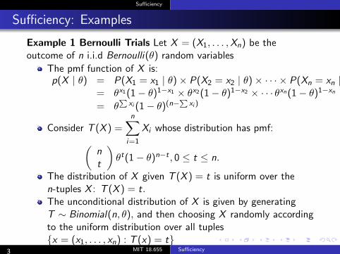
Example 1 Bernoulli Trials Let X = (X1, . . . , Xn) be the outcome of n i.i.d Bernoulli(θ) random variables

The pmf function of X is: p(X | θ) = P(X1 = x1 | θ) × P(X2 = x2 | θ) × · · · × P(Xn = xn

= θx1 (1 − θ)1−x1 × θx2 (1 − θ)1−x2 × · · · θxn (1 − θ)1−xn = θ xi (1 − θ)(n− xi )

nn Consider T (X ) = Xi whose distribution has pmf:

i=1 n

θt (1 − θ)n−t , 0 ≤ t ≤ n. t

The distribution of X given T (X ) = t is uniform over the n-tuples X : T (X ) = t. The unconditional distribution of X is given by generating T ∼ Binomial(n, θ), and then choosing X randomly according to the uniform distribution over all tuples

|

MIT 18.655

} Sufficiency

{x = (x1, . . . , xn) : T (x) = t3

Sufficiency

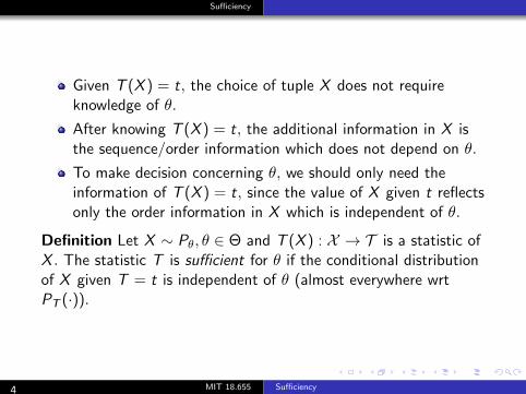
Given T (X ) = t, the choice of tuple X does not require knowledge of θ.

After knowing T (X ) = t, the additional information in X is the sequence/order information which does not depend on θ.

To make decision concerning θ, we should only need the information of T (X ) = t, since the value of X given t reflects only the order information in X which is independent of θ.

Definition Let X ∼ Pθ, θ ∈ Θ and T (X ) : X → T is a statistic of X . The statistic T is sufficient for θ if the conditional distribution of X given T = t is independent of θ (almost everywhere wrt PT (·)).


Sufficiency

Sufficiency Examples

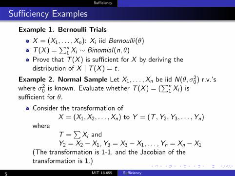
Example 1. Bernoulli Trials

X = (X1, . . . , Xn): Xi iid Bernoulli(θ) nT (X ) = Xi ∼ Binomial(n, θ)1

Prove that T (X ) is sufficient for X by deriving the distribution of X | T (X ) = t.

Example 2. Normal Sample Let X1, . . . , Xn be iid N(θ, σ02) r.v.’s nwhere σ2 is known. Evaluate whether T (X ) = ( Xi ) is 0 1

sufficient for θ.

Consider the transformation of X = (X1, X2, . . . , Xn) to Y = (T , Y2, Y3, . . . , Yn)

where T = Xi and Y2 = X2 − X1, Y3 = X3 − X1, . . . , Yn = Xn − X1

(The transformation is 1-1, and the Jacobian of the transformation is 1.)


Sufficiency

20In).The joint distribution of X | θ is Nn(µ × 1, σ

The joint distribution of Y | θ is Nn

= (nθ, 0, 0, . . . , 0)T ⎡

(µY , ΣYY ) µY ⎤

20nσ 0 0 0 · · · 0 ⎢⎢⎢⎢⎢⎢⎢⎣ . . .

⎥⎥⎥⎥⎥⎥⎥⎦

20 σ20

20

20σ · · · σ

· · · σ· · · σ

20 2σ20

20

20σ

20 σ20 2σ20

20

. . . . . . .. .

0 2σ0 σ

ΣYY = 0 σ

20 σ20 σ20 2σ200 σ

T and (Y2, . . . , Yn) are independent =⇒ (Y2, . . . , Yn) given T = t is

the unconditional distribution =⇒ T is a sufficient statistic for θ.

Note: all functions of (Y2, . . . , Yn) are independent of θ and ¯T , which yields independence of X and s2 :

(Xi − X̄ )2 = 1 1 [ 1 n

n j=1(Xi − Xj )]

22 n n s = i=1 i=1n n


∑ ∑ ∑

Sufficiency

Sufficiency Examples

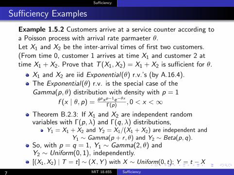
Example 1.5.2 Customers arrive at a service counter according to a Poisson process with arrival rate parmaeter θ. Let X1 and X2 be the inter-arrival times of first two customers. (From time 0, customer 1 arrives at time X1 and customer 2 at time X1 + X2. Prove that T (X1, X2) = X1 + X2 is sufficient for θ.

X1 and X2 are iid Exponential(θ) r.v.’s (by A.16.4). The Exponential(θ) r.v. is the special case of the Gamma(p, θ) distribution with density with p = 1

p−1 −θxx ef (x | θ, p) = θp

, 0 < x < ∞Γ(p)

Theorem B.2.3: If X1 and X2 are independent random variables with Γ(p, λ) and Γ(q, λ) distributions,

Y1 = X1 + X2 and Y2 = X1/(X1 + X2) are independent and Y1 ∼ Gamma(p + r , θ) and Y2 ∼ Beta(p, q).

So, with p = q = 1, Y1 ∼ Gamma(2, θ) and Y2 ∼ Uniform(0, 1), independently.

MIT 18.655 Sufficiency

[(X1, X2) | T = t] ∼ (X , Y ) with X ∼ Uniform(0, t); Y = t − X

7

Sufficiency

Sufficiency: Factorization Theorem

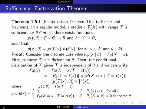
Theorem 1.5.1 (Factorization Theorem Due to Fisher and Neyman). In a regular model, a statistic T (X ) with range T is sufficient for θ ∈ Θ, iff there exists functions

g(t, θ) : T × Θ → R and h : X → R, such that

p(x | θ) = g(T (x), θ)h(x), for all x ∈ X and θ ∈ Θ. Proof: Consider the discrete case where p(x | θ) = Pθ(X = x). First, suppose T is sufficient for θ. Then, the conditional distribution of X given T is independent of θ and we can write

Pθ(x) = Pθ(X = x , T = t(x)) = [Pθ(T = t(x))] × [P(X = x | T = t(x))] = [g(T (x), θ)] × [h(x)]

where g(t, θ) = Pθ(T = t) 0, if Pθ(x) = 0, for all θ

and h(x) =Pθ(X = x | T = t(x)), if Pθ(X = x) > 0 for some θ


Sufficiency


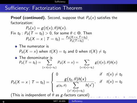
Proof (continued). Second, suppose that Pθ(x) satisfies the factorization:

Pθ(x) = g(t(x), θ)h(x). Fix t0 : Pθ(T = t0) > 0, for some θ ∈ Θ. Then

Pθ (X =x ,T =t0)Pθ(X = x | T = t0) = .Pθ (T =t0)

The numerator is Pθ(X = x) when t(X ) = t0 and 0 when t(X ) = t0

The denominator is Pθ(T = t0) = Pθ(X = x) = g(t(x), θ)h(x)

n n

n

{x :t(x)=t0} {x :t(x)=t0}

0 if t(x) = t0

g(t0, θ)h(x)

⎧ ⎪⎪⎨ if t(x) = t0Pθ(X = x | T = t0) = ,

h(x _)⎪⎪⎩ g (t0, θ)

{x ':t(x)=t0}(This is independent of θ as g -factors cancel)


Sufficiency


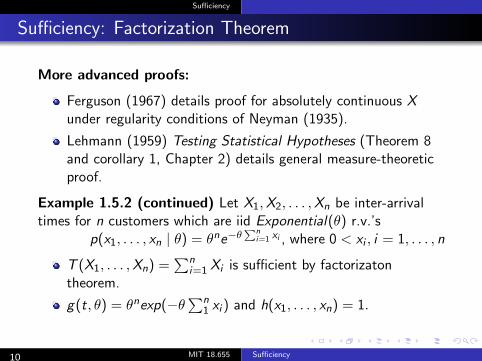
More advanced proofs:

Ferguson (1967) details proof for absolutely continuous X under regularity conditions of Neyman (1935).

Lehmann (1959) Testing Statistical Hypotheses (Theorem 8 and corollary 1, Chapter 2) details general measure-theoretic proof.

Example 1.5.2 (continued) Let X1, X2, . . . , Xn be inter-arrival times for n customers which are iid Exponential(θ) r.v.’s

−θp(x1, . . . , xn | θ) = θne in =1 xi , where 0 < xi , i = 1, . . . , n

nT (X1, . . . , Xn) = i=1 Xi is sufficient by factorizaton theorem.

n g(t, θ) = θnexp(−θ 1 xi ) and h(x1, . . . , xn) = 1.


∑∑∑

Sufficiency

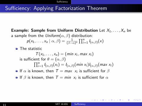
Sufficiency: Applying Factorization Theorem

Example: Sample from Uniform Distribution Let X1, . . . , Xn be a sample from the Uniform(α, β) distribution: e

p(x1, . . . , xn | α, β) = 1 (β−α)n

n i=1 I(α,β)(x)

The statistic T (x1, . . . , xn) = (min xi , max xi )

is sufficient for θ = (α, β)e n I(α,β)(xi ) = I(α,β)(min xi )I(α,β)(max xi )i=1

If α is known, then T = max xi is sufficient for β

If β is known, then T = min xi is sufficient for α


Sufficiency


Example 1.5.4 Normal Sample. Let X1, . . . , Xn be iid N(µ, σ2), with unknown θ = (µ, σ2) ∈ R × R+

The joint density is e n √ 1 1p(x1, . . . , xn | θ) = exp(− (xi − µ)2)i=1 2σ22πσ2

= (2πσ2)−n/2exp(−nµ2) 2σ2 )× 1 n 2 n exp − − 2µ

2σ2 ( i=1 xi i=1 xi )n n = g( 2 i=1 xi , i=1 xi ; θ)

n nT (X1, . . . , Xn) = ( Xi , X 2) is sufficient. i=1 i=1 i

T ∗(X1, . . . , Xn) = ( X̄ , s2) is sufficient, where 1 n 2 1 nX̄ = Xi , s = (Xi − X̄ )2) are sufficient. n i=1 (n−1) i=1

Note: Sufficient statistics are not unique (their level sets are!!).


∑ ∑∑ ∑∑ ∑∑ ∑

Sufficiency


Example 1.5.5 Normal linear regression model. Let Y1, . . . , Yn be independent with Yi ∼ N(µi , σ

2), where µi = β1 + β2zi , i = 1, 2, . . . , n

and zi are constants.

Under what conditions is θ = (β1, β2, σ2) identifiable?

Under those conditions, the joint density for (Y1, . . . , Yn) is e n √ 1 1 p(y1, . . . , yn | θ) = exp(−2σ2 (yi − µi )

2)i=1 2πσ2

1 n = (2πσ2)−n/2exp(− (yi − β1 − β2zi )2 2σ2 i=11 n = (2πσ2)−n/2exp(− (β1 + β2zi )2)2σ2 i=1

1 n 2×exp(− (y − 2(β1 + β2zi )yi ))2σ2 i=1 i which equals

1 n(2πσ2)−n/2exp(− (β1 + β2zi )2)2σ2 i=11 n 2 n n×exp(− [( ) − 2β1(2σ2 i=1 yi i=1 yi ) − 2β2( i=1 zi yi ))

n n nT = ( Y 2 , Yi , i=1 zi Yi ) is sufficient for θi=1 i i=1


∑∑∑∑ ∑ ∑∑ ∑ ∑

∑

Sufficiency

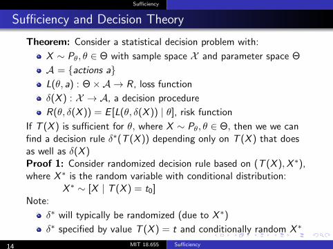
Sufficiency and Decision Theory

Theorem: Consider a statistical decision problem with:

X ∼ Pθ, θ ∈ Θ with sample space X and parameter space Θ

A = {actions a}L(θ, a) : Θ ×A → R, loss function

δ(X ) : X → A, a decision procedure

R(θ, δ(X )) = E [L(θ, δ(X )) | θ], risk function

If T (X ) is sufficient for θ, where X ∼ Pθ, θ ∈ Θ, then we we can find a decision rule δ∗(T (X )) depending only on T (X ) that does as well as δ(X ) Proof 1: Consider randomized decision rule based on (T (X ), X ∗), where X ∗ is the random variable with conditional distribution:

X ∗ ∼ [X | T (X ) = t0] Note:

δ∗ will typically be randomized (due to X ∗)

δ∗ specified by value T (X ) = t and conditionally random X ∗


Sufficiency

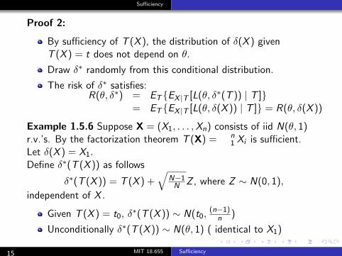
Proof 2:

By sufficiency of T (X ), the distribution of δ(X ) given T (X ) = t does not depend on θ.

Draw δ∗ randomly from this conditional distribution.

The risk of δ∗ satisfies: R(θ, δ∗) = ET {EX |T [L(θ, δ

∗(T )) | T ]}= ET {EX |T [L(θ, δ(X )) | T ]} = R(θ, δ(X ))

Example 1.5.6 Suppose X = (X1, . . . , Xn) consists of iid N(θ, 1) nr.v.’s. By the factorization theorem T (X) = Xi is sufficient. 1

Let δ(X ) = X1. Define δ∗(T (X )) as follows

N−1δ∗(T (X )) = T (X ) + Z , where Z ∼ N(0, 1),N independent of X .

(n−1)Given T (X ) = t0, δ∗(T (X )) ∼ N(t0, )n

Unconditionally δ∗(T (X )) ∼ N(θ, 1) ( identical to X1)


Sufficiency

Sufficiency and Bayes Models

Definition: Let X ∼ Pθ, θ ∈ Θ and let Π be the Prior distribution on Θ. The statistic T (X ) is Bayes sufficient for Π if

Π(θ | X = x), the Posterior distribution of θ given X is the same as

Π(θ | T (X ) = t(x)), the Posterior distribution of θ given T (X ) for all x .

Theorem 1.5.2 (Kolmogorov). If T (X ) is sufficient for θ, then it is Bayes sufficient for every prior distribution Π. Proof Problem 1.5.14.


Sufficiency

Minimal Sufficiency

Issue: Probability models often admit many sufficient statistics. Suppose X = (X1, . . . , Xn) where Xi are iid Pθ, θ ∈ Θ.

T (X ) = (X1, . . . , Xn) is (trivially) sufficient

T _(X ) = (X[1], X[2], . . . , X[n]) where X[j ] = j-th smallest {Xi }(j-th order statistic) is sufficient

T _(X ) provides a greater reduction of the data. ¯If the Xi are iid N(θ, 1) then T

'' = X is sufficient.

Definition A statistic T (X ) is minimally sufficient if it is sufficient and provides a greater reduction of the data than any other sufficient statistic. If S(X ) is any sufficient statistic, then there exists a mapping r :

T (X ) = r(S(X ))


Sufficiency

Minimal Sufficiency: Example

Example 1.5.1 (continued). X1, . . . , Xn are iid Bernoulli(θ) and nT = 1 Xi is sufficient.

Let S(X ) be any other sufficient statistic. By the factorization therem:

p(x | θ) = g(S(x), θ)h(x), for some functions g(·, ·) and h(·). Using the pmf of X we have

θT (1 − θ)(n−T ) = g(S(x), θ)h(x), for all θ ∈ [0, 1] Fix any two values of θ, say θ1 and θ2 and take the ratio of the pmfs:

(θ1/θ2)T [(1 − θ1)/(1 − θ2)]n−T = g(S(x), θ1)/g(S(x), θ2)

Take logarithm of both sides and solve for T . E.g., θ1 = 2/3 and θ2 = 1/3

T = r(S(X )) = log [2ng(S(x), θ1)/g(S(x), θ2)]/2log2.


∑

Sufficiency

The Likelihood Function

Definition For X ∼ Pθ, θ ∈ Θ let p(x | θ) be the pmf or density function. The likelihood function L for a given observed data value X = x is

Lx (θ) = p(x | θ), θ ∈ Θ The function L : X to T , the function class

T = {f : θ → p(x | θ), x ∈ X}

Theorem (Dynkin, Lehmann, and Scheffe) Suppose there exists θ0:

{x : p(x | θ) > 0} ⊂ {x : p(x | θ0) > 0} for all θ. Lx (·)Define: Λx (·) = : Θ → R.Lx (θ0)

Then Λx (·) is the function-valued statistic that is minimal sufficient. Proof Problem 1.5.12 Note: As a function, Λx (·) at θ has value p(x | θ)/p(x | θ0), the ratio of likelihoods at θ and at θ0.


Sufficiency

Sufficient Statistics and Ancillary Statistics

Suppose X ∼ Pθ, θ ∈ Θ and that T (X ) is a sufficient statistic. Consider a 1:1 mapping of X which includes the sufficient statistic

X → (T (X ), S(X )). Because the mapping is 1:1, we can recover X given T (X ) = t and S(X ) = s.

T (X ) is sufficient for θ, so S(X ) is irrelevant so long as P={Pθ, θ ∈ Θ} is valid.

Using S(X ) to Evaluate Validity of P

Example 1.5.5: X = (X1, . . . , Xn) iid N(θ, 1) ¯T (X ) = X and S(X ) = (X1 − X̄ , . . . , Xn − X̄ )

To evaluate the validity of Var(Xi ) ≡ 1, we need S(X ). Example 1.5.4: X = (X1, . . . , Xn) iid N(θ, σ2)

n nT (X ) = ( Xi , X 2) or equivalently 1 1 i T (X ) = ( X̄ , s2) To evaluate the validity of the Normal Assumption, we need S(X ). (See Problem 1.5.13)


∑ ∑

MIT OpenCourseWare http://ocw.mit.edu

18.655 Mathematical Statistics Spring 2016

For information about citing these materials or our Terms of Use, visit: http://ocw.mit.edu/terms.

http://ocw.mit.edu/terms

http://ocw.mit.edu/

Mathematical Statistics, Lecture 6 Sufficiency · 2020-01-03 · Suﬃciency Given T (X ) = t, the...

Documents

Transcript of Mathematical Statistics, Lecture 6 Sufficiency · 2020-01-03 · Suﬃciency Given T (X ) = t, the...