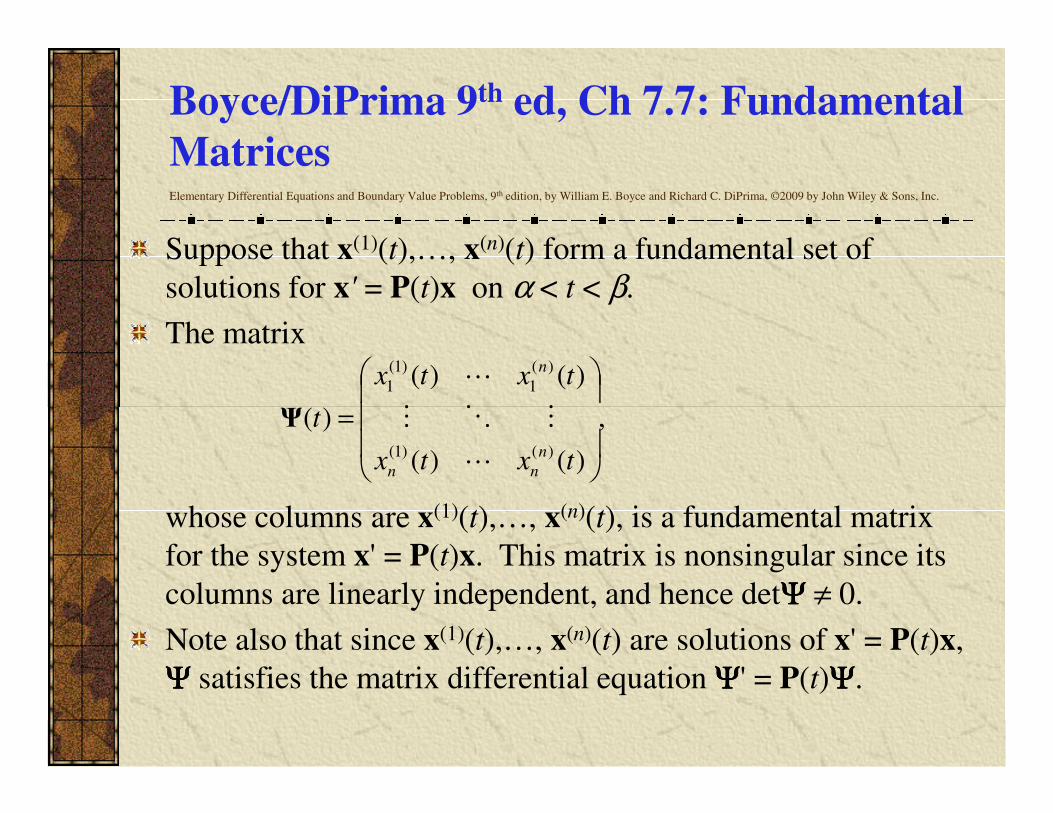
Boyce/DiPrima 9th ed, Ch 7.7: Fundamental

MatricesElementary Differential Equations and Boundary Value Problems, 9th edition, by William E. Boyce and Richard C. DiPrima, ©2009 by John Wiley & Sons, Inc.

Suppose that x(1)(t),…, x(n)(t) form a fundamental set of

solutions for x' = P(t)x on α < t < β.

The matrix

,

)()(

)(

)(

1

)1(

1

=

txtx

t

n

⋮⋱⋮

⋯

Ψ

whose columns are x(1)(t),…, x(n)(t), is a fundamental matrix

for the system x' = P(t)x. This matrix is nonsingular since its

columns are linearly independent, and hence detΨΨΨΨ ≠ 0.

Note also that since x(1)(t),…, x(n)(t) are solutions of x' = P(t)x,

ΨΨΨΨ satisfies the matrix differential equation ΨΨΨΨ' = P(t)ΨΨΨΨ.

,

)()(

)()()1(

=

txtx

tn

nn ⋯

⋮⋱⋮Ψ

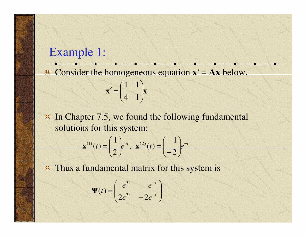
Example 1:

Consider the homogeneous equation x' = Ax below.

In Chapter 7.5, we found the following fundamental

xx

=′

14

11

In Chapter 7.5, we found the following fundamental

solutions for this system:

Thus a fundamental matrix for this system is

ttetet

−

−=

=

2

1)(,

2

1)( )2(3)1( xx

−=

−

−

tt

tt

ee

eet

22)(

3

3

Ψ

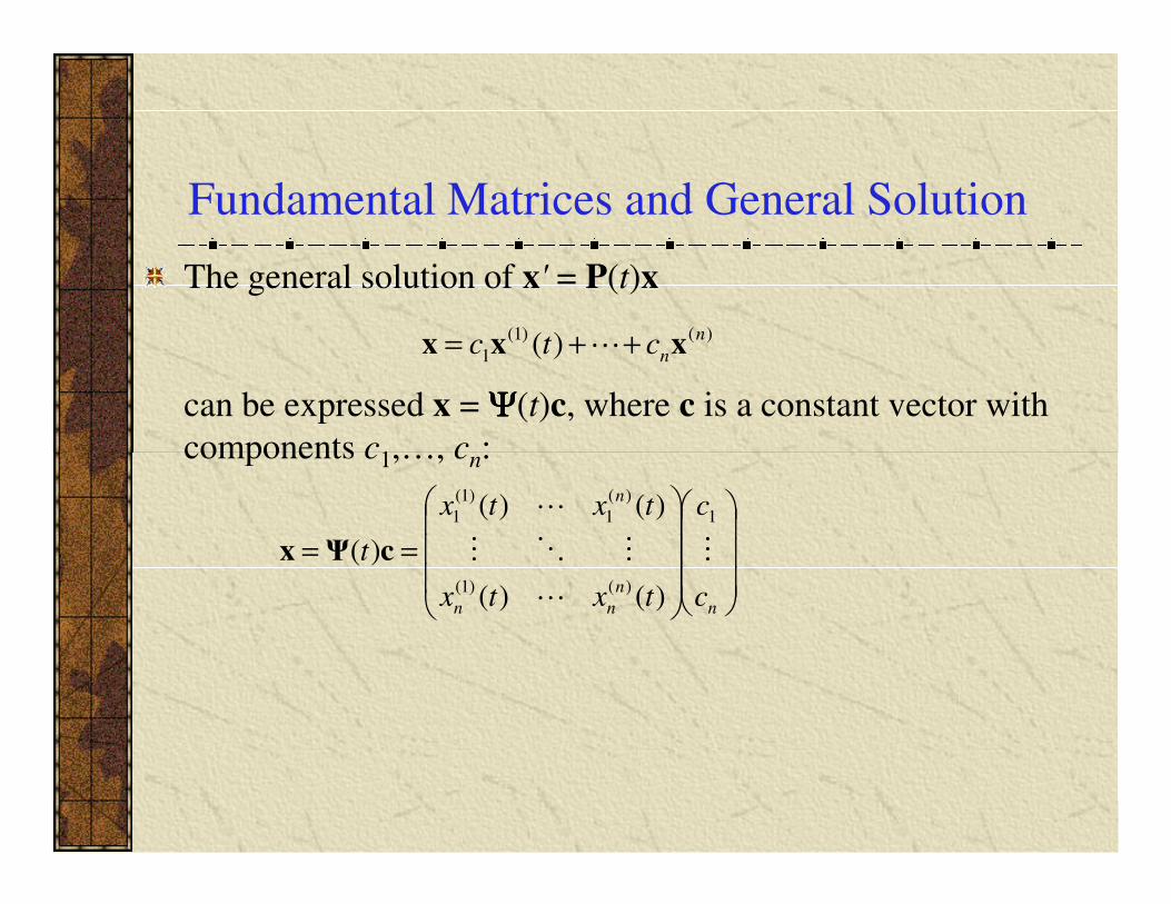
Fundamental Matrices and General Solution

The general solution of x' = P(t)x

can be expressed x = ΨΨΨΨ(t)c, where c is a constant vector with

components c1,…, cn:

)()1(

1 )( n

nctc xxx ++= ⋯

components c1,…, cn:

==

n

n

nn

n

c

c

txtx

txtx

t ⋮

⋯

⋮⋱⋮

⋯ 1

)()1(

)(

1

)1(

1

)()(

)()(

)( cΨx

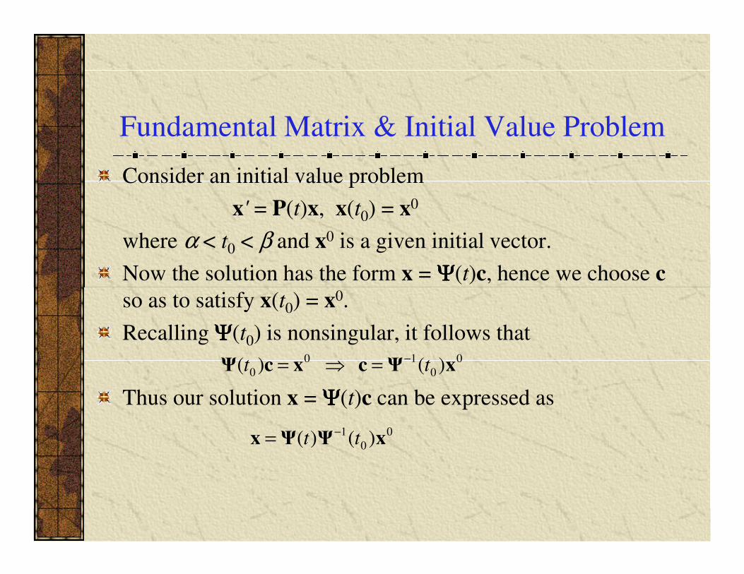
Fundamental Matrix & Initial Value Problem

Consider an initial value problem

x' = P(t)x, x(t0) = x0

where α < t0 < β and x0 is a given initial vector.

Now the solution has the form x = ΨΨΨΨ(t)c, hence we choose c

so as to satisfy x(t ) = x0. so as to satisfy x(t0) = x0.

Recalling ΨΨΨΨ(t0) is nonsingular, it follows that

Thus our solution x = ΨΨΨΨ(t)c can be expressed as

0

0

10

0 )()( xΨcxcΨ tt−=⇒=

0

0

1 )()( xΨΨx tt−=

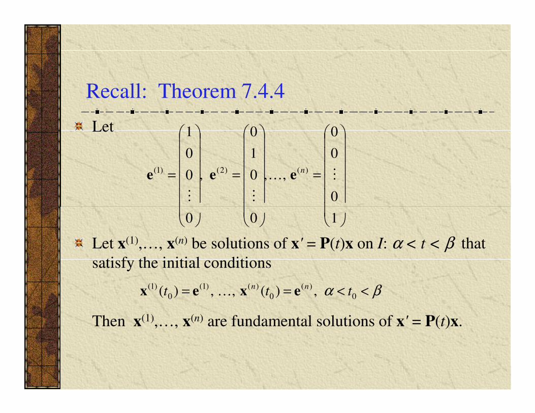
Recall: Theorem 7.4.4

Let

=

=

=

0

0

0

,,0

1

0

,0

0

1

)()2()1(⋮…

⋮⋮

neee

Let x(1),…, x(n) be solutions of x' = P(t)x on I: α < t < β that

satisfy the initial conditions

Then x(1),…, x(n) are fundamental solutions of x' = P(t)x.

100

βα <<== 0

)(

0

)()1(

0

)1( ,)(,,)( tttnn exex …

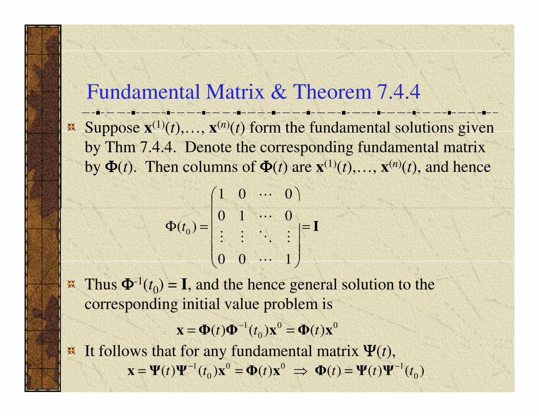
Fundamental Matrix & Theorem 7.4.4

Suppose x(1)(t),…, x(n)(t) form the fundamental solutions given

by Thm 7.4.4. Denote the corresponding fundamental matrix

by ΦΦΦΦ(t). Then columns of ΦΦΦΦ(t) are x(1)(t),…, x(n)(t), and hence

010

001

⋯

⋯

Thus ΦΦΦΦ-1(t0) = I, and the hence general solution to the

corresponding initial value problem is

It follows that for any fundamental matrix ΨΨΨΨ(t),

I=

=Φ

100

010)( 0

⋯

⋮⋱⋮⋮

⋯t

00

0

1 )()()( xΦxΦΦx ttt == −

)()()()()()( 0

100

0

1tttttt

−− =⇒== ΨΨΦxΦxΨΨx

The Fundamental Matrix ΦΦΦΦand Varying Initial Conditions

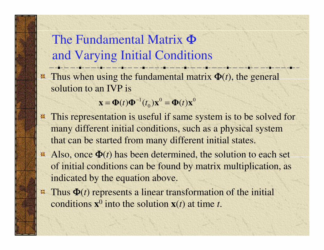
Thus when using the fundamental matrix ΦΦΦΦ(t), the general

solution to an IVP is

This representation is useful if same system is to be solved for

many different initial conditions, such as a physical system

00

0

1 )()()( xΦxΦΦx ttt == −

many different initial conditions, such as a physical system

that can be started from many different initial states.

Also, once ΦΦΦΦ(t) has been determined, the solution to each set

of initial conditions can be found by matrix multiplication, as

indicated by the equation above.

Thus ΦΦΦΦ(t) represents a linear transformation of the initial

conditions x0 into the solution x(t) at time t.

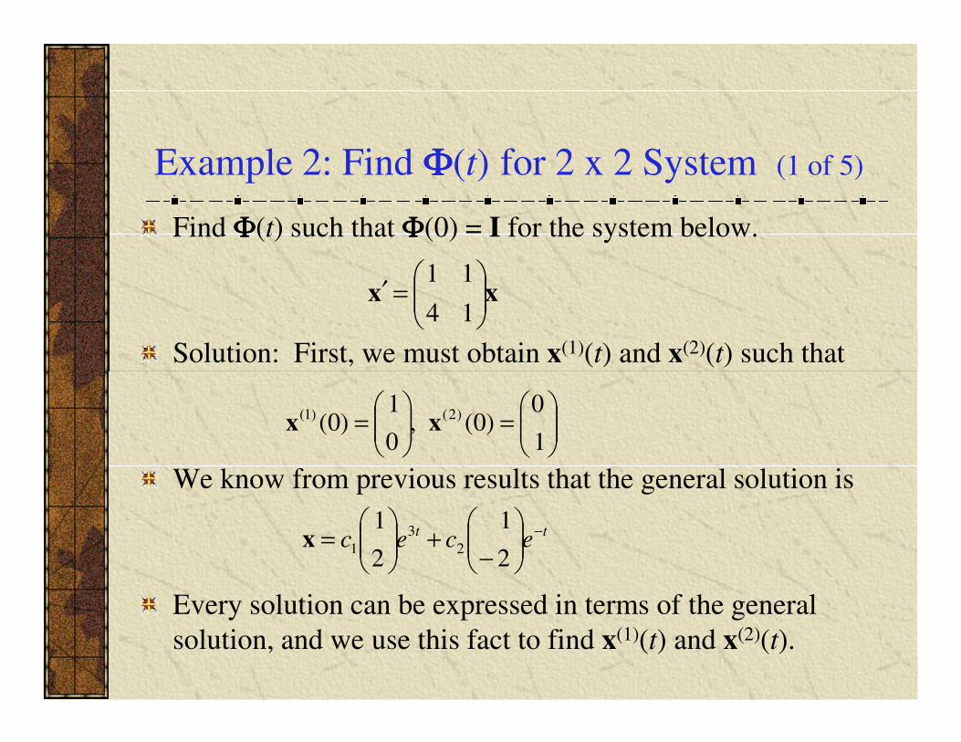
Example 2: Find ΦΦΦΦ(t) for 2 x 2 System (1 of 5)

Find ΦΦΦΦ(t) such that ΦΦΦΦ(0) = I for the system below.

Solution: First, we must obtain x(1)(t) and x(2)(t) such that

xx

=′

14

11

We know from previous results that the general solution is

Every solution can be expressed in terms of the general

solution, and we use this fact to find x(1)(t) and x(2)(t).

ttecec

−

−+

=

2

1

2

12

3

1x

=

=

1

0)0(,

0

1)0( )2()1( xx

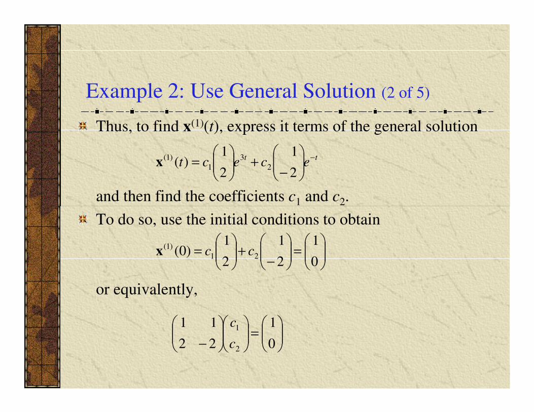
Example 2: Use General Solution (2 of 5)

Thus, to find x(1)(t), express it terms of the general solution

and then find the coefficients c1 and c2.

ttecect

−

−+

=

2

1

2

1)( 2

3

1

)1(x

1 2

To do so, use the initial conditions to obtain

or equivalently,

=

−+

=

0

1

2

1

2

1)0( 21

)1(ccx

=

− 0

1

22

11

2

1

c

c

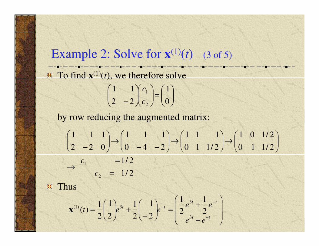
Example 2: Solve for x(1)(t) (3 of 5)

To find x(1)(t), we therefore solve

by row reducing the augmented matrix:

=

− 0

1

22

11

2

1

c

c

Thus

2/1

2/1

2/110

2/101

2/110

111

240

111

022

111

2

1

=

=→

→

→

−−→

−

c

c

−

+=

−+

=

−

−−

tt

tttt

ee

eeeet

3

33)1(

2

1

2

1

2

1

2

1

2

1

2

1)(x

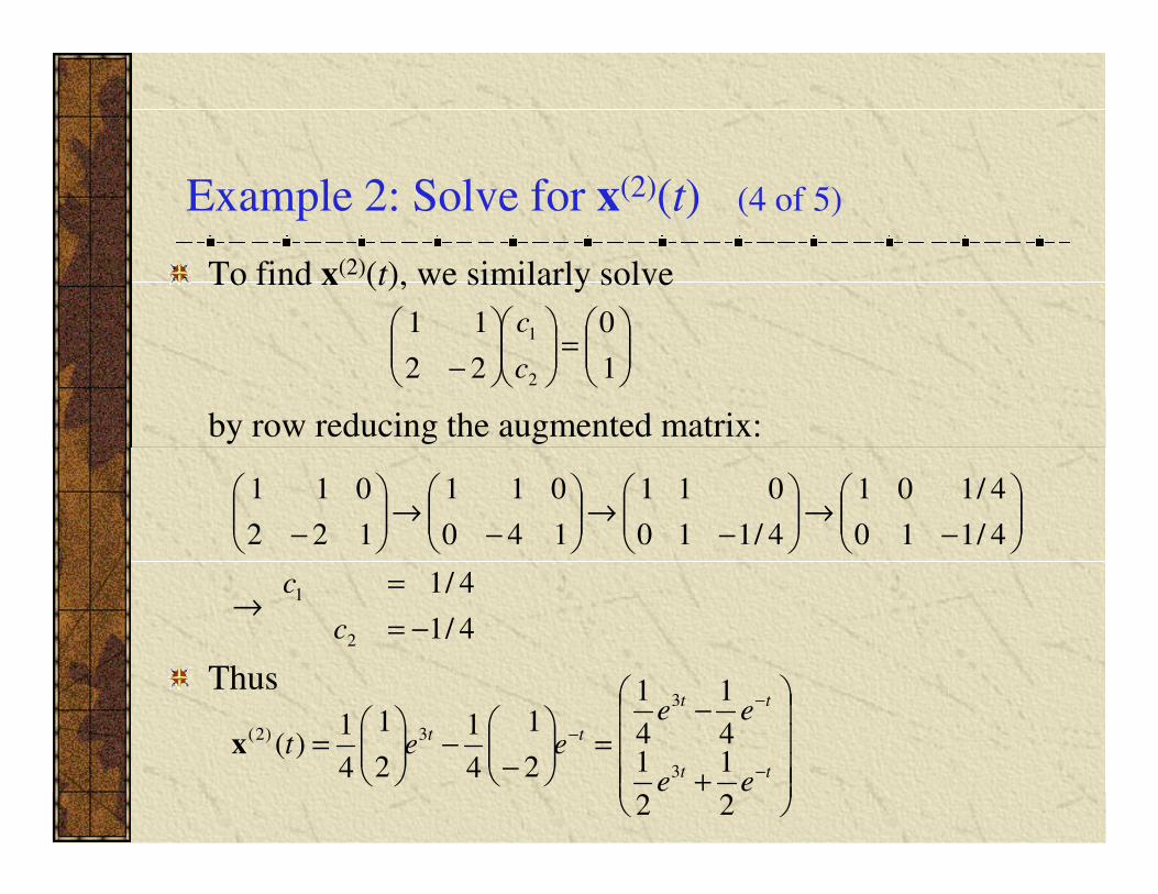
Example 2: Solve for x(2)(t) (4 of 5)

To find x(2)(t), we similarly solve

by row reducing the augmented matrix:

=

− 1

0

22

11

2

1

c

c

Thus

4/1

4/1

4/110

4/101

4/110

011

140

011

122

011

2

1

−=

=→

−→

−→

−→

−

c

c

+

−=

−−

=

−

−

−

tt

tt

tt

ee

eeeet

2

1

2

14

1

4

1

2

1

4

1

2

1

4

1)(

3

3

3)2(x

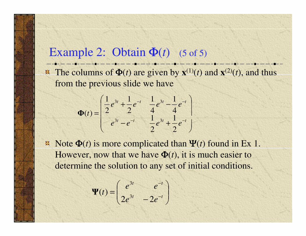
Example 2: Obtain ΦΦΦΦ(t) (5 of 5)

The columns of ΦΦΦΦ(t) are given by x(1)(t) and x(2)(t), and thus

from the previous slide we have

+−

−+=

−−

−−

tttt

tttteeee

t114

1

4

1

2

1

2

1

)(33

33

Φ

Note ΦΦΦΦ(t) is more complicated than ΨΨΨΨ(t) found in Ex 1.

However, now that we have ΦΦΦΦ(t), it is much easier to

determine the solution to any set of initial conditions.

+− −− tttteeee

2

1

2

1 33

−=

−

−

tt

tt

ee

eet

22)(

3

3

Ψ

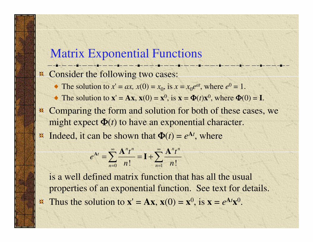
Matrix Exponential Functions

Consider the following two cases:

The solution to x' = ax, x(0) = x0, is x = x0eat, where e0 = 1.

The solution to x' = Ax, x(0) = x0, is x = ΦΦΦΦ(t)x0, where ΦΦΦΦ(0) = I.

Comparing the form and solution for both of these cases, we

might expect ΦΦΦΦ(t) to have an exponential character. might expect ΦΦΦΦ(t) to have an exponential character.

Indeed, it can be shown that ΦΦΦΦ(t) = eAt, where

is a well defined matrix function that has all the usual

properties of an exponential function. See text for details.

Thus the solution to x' = Ax, x(0) = x0, is x = eAtx0.

∑∑∞

=

∞

=

+==10 !! n

nn

n

nnt

n

t

n

te

AI

AA

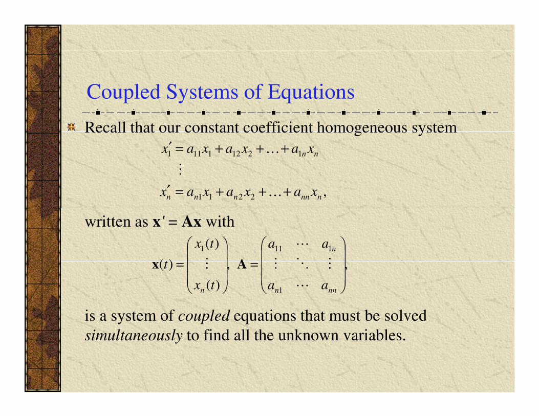
Coupled Systems of Equations

Recall that our constant coefficient homogeneous system

,2211

12121111

nnnnnn

nn

xaxaxax

xaxaxax

+++=′

+++=′

…

⋮

…

written as x' = Ax with

is a system of coupled equations that must be solved

simultaneously to find all the unknown variables.

,,

)(

)(

)(

1

1111

=

=

nnn

n

n aa

aa

tx

tx

t

⋯

⋮⋱⋮

⋯

⋮ Ax

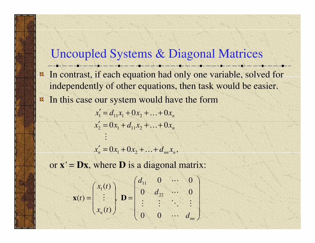
Uncoupled Systems & Diagonal Matrices

In contrast, if each equation had only one variable, solved for

independently of other equations, then task would be easier.

In this case our system would have the form

00

00 21111 n

xxdxx

xxxdx

+++=′

+++=′

…

…

or x' = Dx, where D is a diagonal matrix:

,00

00

21

21112

nnnn

n

xdxxx

xxdxx

+++=′

+++=′

…

⋮

…

=

=

nn

nd

d

d

tx

tx

t

⋯

⋮⋱⋮⋮

⋯

⋯

⋮

00

00

00

,

)(

)(

)(22

11

1

Dx

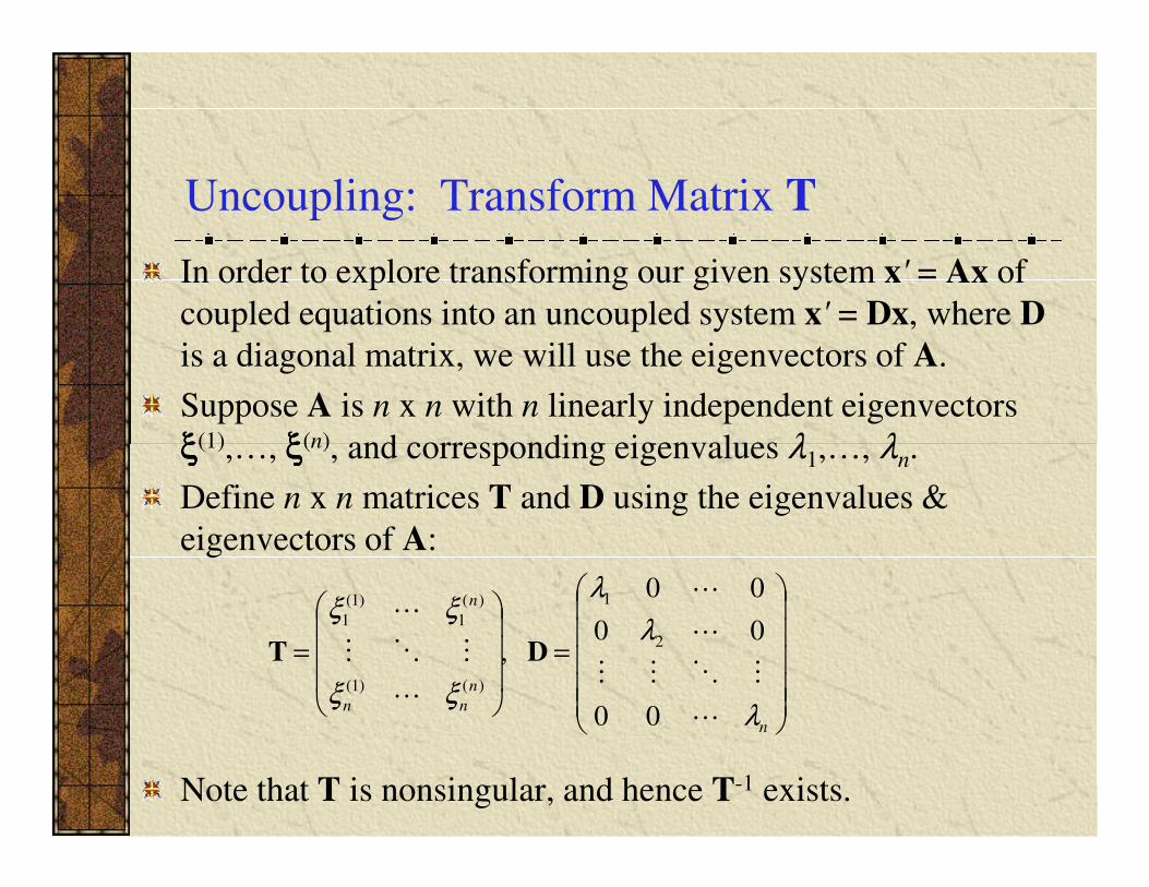
Uncoupling: Transform Matrix T

In order to explore transforming our given system x' = Ax of

coupled equations into an uncoupled system x' = Dx, where D

is a diagonal matrix, we will use the eigenvectors of A.

Suppose A is n x n with n linearly independent eigenvectors

ξξξξ(1),…, ξξξξ(n), and corresponding eigenvalues λ ,…, λ .ξξξξ(1),…, ξξξξ(n), and corresponding eigenvalues λ1,…, λn.

Define n x n matrices T and D using the eigenvalues &

eigenvectors of A:

Note that T is nonsingular, and hence T-1 exists.

=

=

n

n

nn

n

λ

λ

λ

ξξ

ξξ

⋯

⋮⋱⋮⋮

⋯

⋯

⋯

⋮⋱⋮

⋯

00

00

00

,2

1

)()1(

)(

1

)1(

1

DT

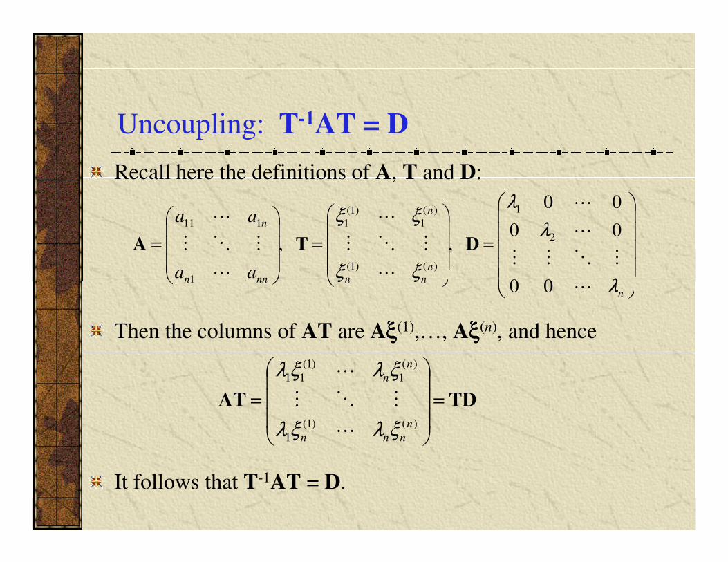
Uncoupling: T-1AT = D

Recall here the definitions of A, T and D:

=

=

=n

nn

n

nnn

n

aa

aa

λ

λ

λ

ξξ

ξξ

⋯

⋮⋱⋮⋮

⋯

⋯

⋯

⋮⋱⋮

⋯

⋯

⋮⋱⋮

⋯

00

00

00

,,2

1

)()1(

)(

1

)1(

1

1

111

DTA

Then the columns of AT are Aξξξξ(1),…, Aξξξξ(n), and hence

It follows that T-1AT = D.

n

nnnnn aaλ

ξξ⋯

⋯⋯00

1

TDAT =

=)()1(

1

)(

1

)1(

11

n

nnn

n

n

ξλξλ

ξλξλ

⋯

⋮⋱⋮

⋯

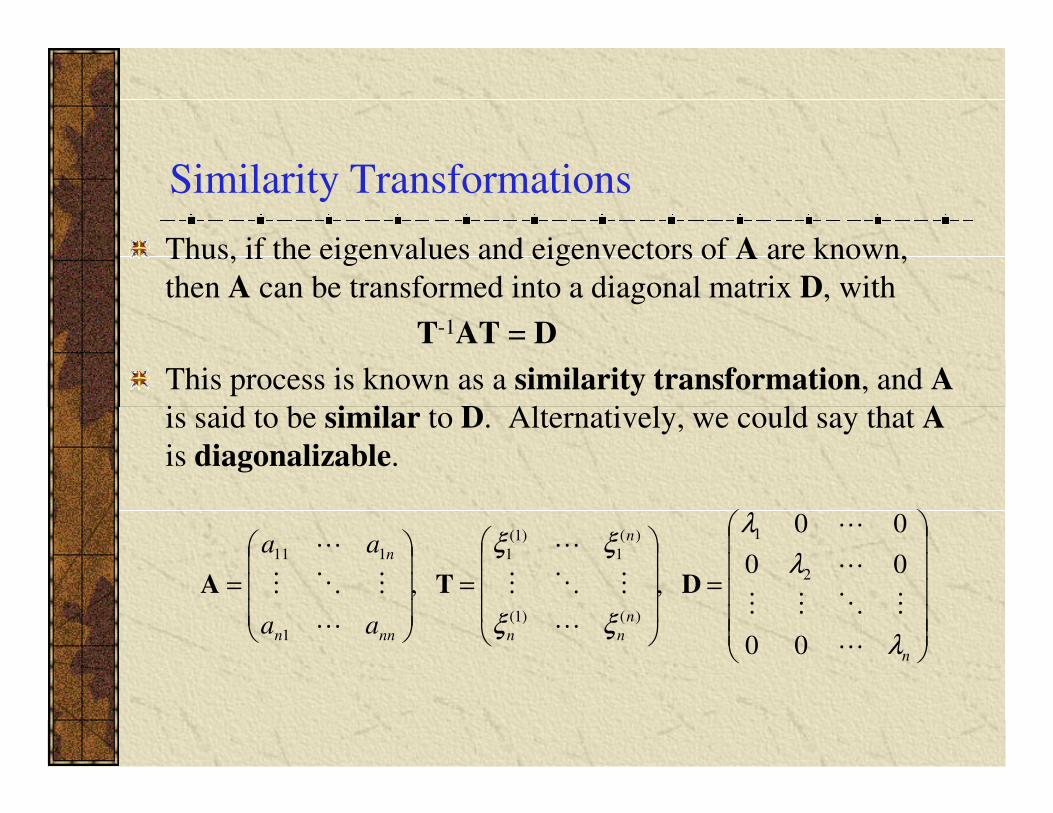
Similarity Transformations

Thus, if the eigenvalues and eigenvectors of A are known,

then A can be transformed into a diagonal matrix D, with

T-1AT = D

This process is known as a similarity transformation, and A

is said to be similar to D. Alternatively, we could say that Ais said to be similar to D. Alternatively, we could say that A

is diagonalizable.

=

=

=

n

n

nn

n

nnn

n

aa

aa

λ

λ

λ

ξξ

ξξ

⋯

⋮⋱⋮⋮

⋯

⋯

⋯

⋮⋱⋮

⋯

⋯

⋮⋱⋮

⋯

00

00

00

,,2

1

)()1(

)(

1

)1(

1

1

111

DTA

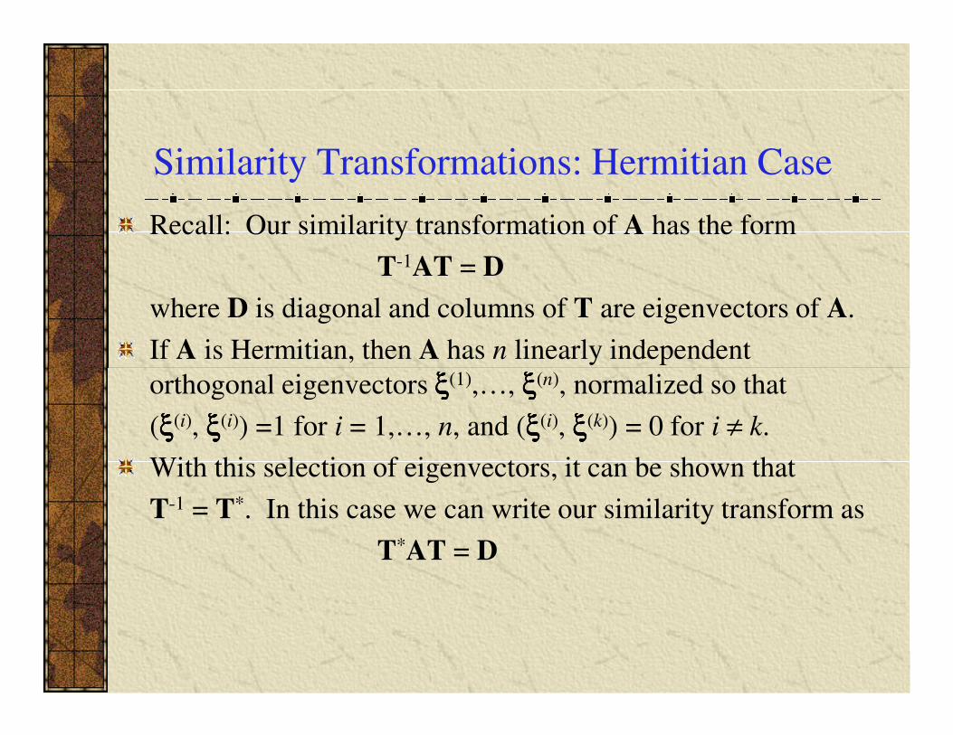
Similarity Transformations: Hermitian Case

Recall: Our similarity transformation of A has the form

T-1AT = D

where D is diagonal and columns of T are eigenvectors of A.

If A is Hermitian, then A has n linearly independent

orthogonal eigenvectors ξξξξ(1),…, ξξξξ(n), normalized so that orthogonal eigenvectors ξξξξ(1),…, ξξξξ(n), normalized so that

(ξξξξ(i), ξξξξ(i)) =1 for i = 1,…, n, and (ξξξξ(i), ξξξξ(k)) = 0 for i ≠ k.

With this selection of eigenvectors, it can be shown that

T-1 = T*. In this case we can write our similarity transform as

T*AT = D

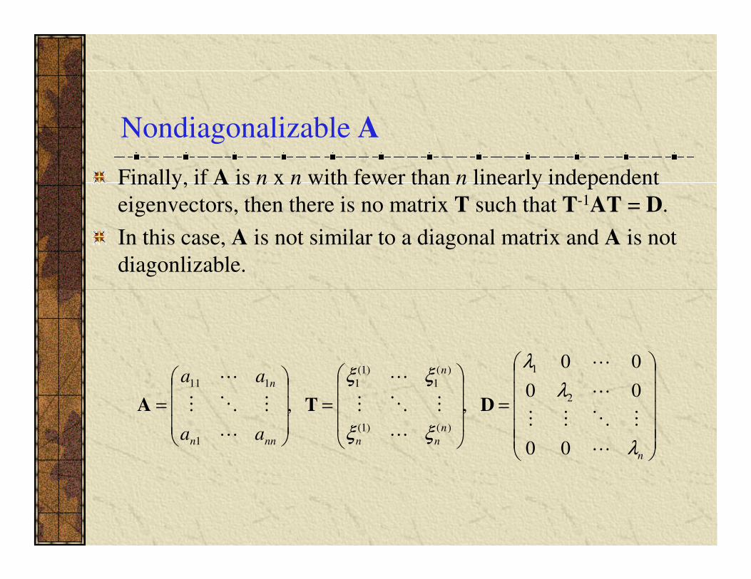
Nondiagonalizable A

Finally, if A is n x n with fewer than n linearly independent

eigenvectors, then there is no matrix T such that T-1AT = D.

In this case, A is not similar to a diagonal matrix and A is not

diagonlizable.

=

=

=

n

n

nn

n

nnn

n

aa

aa

λ

λ

λ

ξξ

ξξ

⋯

⋮⋱⋮⋮

⋯

⋯

⋯

⋮⋱⋮

⋯

⋯

⋮⋱⋮

⋯

00

00

00

,,2

1

)()1(

)(

1

)1(

1

1

111

DTA

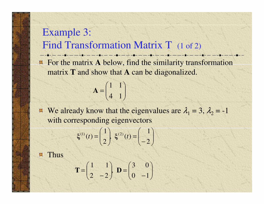
Example 3:

Find Transformation Matrix T (1 of 2)

For the matrix A below, find the similarity transformation

matrix T and show that A can be diagonalized.

=

14

11A

We already know that the eigenvalues are λ1 = 3, λ2 = -1

with corresponding eigenvectors

Thus

−=

=

2

1)(,

2

1)( )2()1(

tt ξξ

−=

−=

10

03,

22

11DT

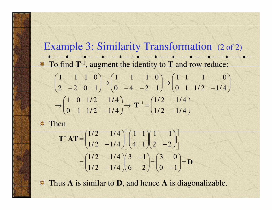
Example 3: Similarity Transformation (2 of 2)

To find T-1, augment the identity to T and row reduce:

=→

→

−→

−−→

−

− 4/12/14/12/101

4/12/110

0111

1240

0111

1022

0111

1T

Then

Thus A is similar to D, and hence A is diagonalizable.

−

=→

−

→4/12/14/12/110

1T

D

ATT

=

−=

−

−=

−

−=−

10

03

26

13

4/12/1

4/12/1

22

11

14

11

4/12/1

4/12/11

Fundamental Matrices for Similar Systems (1 of 3)

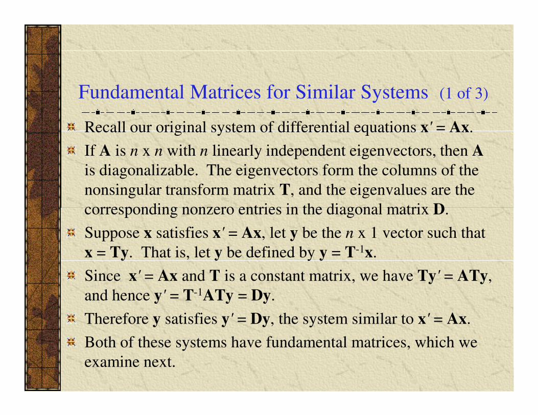
Recall our original system of differential equations x' = Ax.

If A is n x n with n linearly independent eigenvectors, then A

is diagonalizable. The eigenvectors form the columns of the

nonsingular transform matrix T, and the eigenvalues are the

corresponding nonzero entries in the diagonal matrix D.corresponding nonzero entries in the diagonal matrix D.

Suppose x satisfies x' = Ax, let y be the n x 1 vector such that

x = Ty. That is, let y be defined by y = T-1x.

Since x' = Ax and T is a constant matrix, we have Ty' = ATy,

and hence y' = T-1ATy = Dy.

Therefore y satisfies y' = Dy, the system similar to x' = Ax.

Both of these systems have fundamental matrices, which we

examine next.

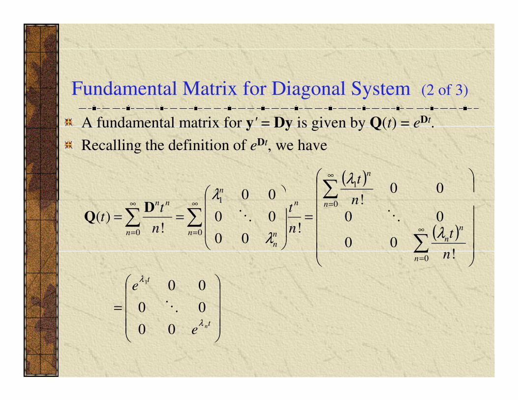
Fundamental Matrix for Diagonal System (2 of 3)

A fundamental matrix for y' = Dy is given by Q(t) = eDt.

Recalling the definition of eDt, we have

( )

∑

∞

=∞∞ n

n

n

n

nn n

t

tt

λλ 00

!000

1

1D

( )

=

=

==

∑

∑

∑∑∞

=

=∞

=

∞

=

t

t

n

n

n

n

n

n

n

n

n

nn

ne

e

n

t

n

n

t

n

tt

λ

λ

λλ

λ

00

00

00

!00

00

!

!00

00

00

!)(

1

0

0

0

1

0

⋱

⋱⋱D

Q

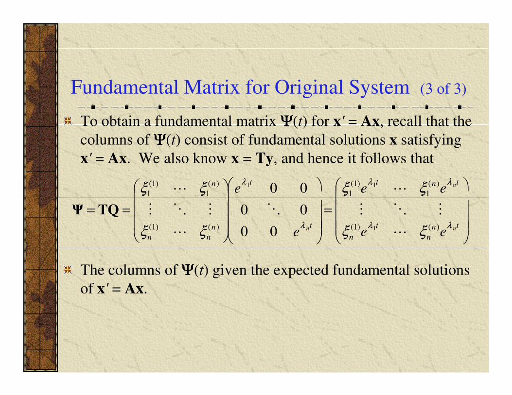
Fundamental Matrix for Original System (3 of 3)

To obtain a fundamental matrix ΨΨΨΨ(t) for x' = Ax, recall that the

columns of ΨΨΨΨ(t) consist of fundamental solutions x satisfying

x' = Ax. We also know x = Ty, and hence it follows that

tnttn neee

λλλξξξξ )(

1

)1(

1

)(

1

)1(

111 00 ⋯⋯

The columns of ΨΨΨΨ(t) given the expected fundamental solutions

of x' = Ax.

=

==tn

n

t

n

tn

nn

nn eeeλλλ

ξξξξ )()1(

11

)()1(

11

100

00

⋯

⋮⋱⋮

⋯

⋱

⋯

⋮⋱⋮

⋯

TQΨ

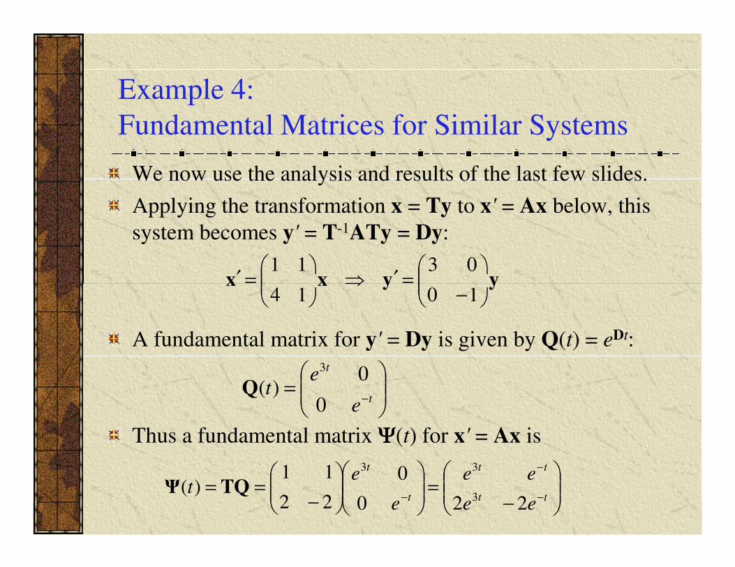
Example 4:

Fundamental Matrices for Similar Systems

We now use the analysis and results of the last few slides.

Applying the transformation x = Ty to x' = Ax below, this

system becomes y' = T-1ATy = Dy:

yyxx

−=′⇒

=′10

03

14

11

A fundamental matrix for y' = Dy is given by Q(t) = eDt:

Thus a fundamental matrix ΨΨΨΨ(t) for x' = Ax is

yyxx

−

=′⇒

=′1014

=

−t

t

e

et

0

0)(

3

Q

−=

−==

−

−

− tt

tt

t

t

ee

ee

e

et

220

0

22

11)(

3

33

TQΨ