Lecture Notes

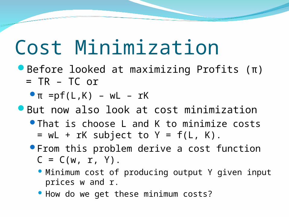
Cost MinimizationBefore looked at maximizing Profits (π) = TR

– TC orπ =pf(L,K) – wL – rK

But now also look at cost minimizationThat is choose L and K to minimize costs = wL

+ rK subject to Y = f(L, K).From this problem derive a cost function C =

C(w, r, Y). Minimum cost of producing output Y given input

prices w and r. How do we get these minimum costs?

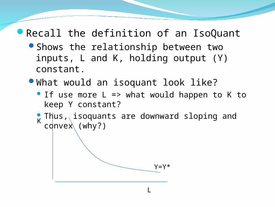
Recall the definition of an IsoQuantShows the relationship between two inputs, L

and K, holding output (Y) constant.What would an isoquant look like?

If use more L => what would happen to K to keep Y constant?

Thus, isoquants are downward sloping and convex (why?)

L

K

Y=Y*

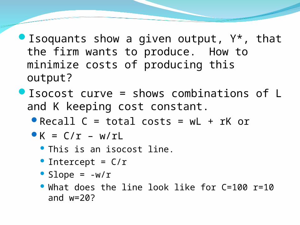
Isoquants show a given output, Y*, that the firm wants to produce. How to minimize costs of producing this output?

Isocost curve = shows combinations of L and K keeping cost constant.Recall C = total costs = wL + rK orK = C/r – w/rL

This is an isocost line. Intercept = C/r Slope = -w/r What does the line look like for C=100 r=10 and

w=20?

K

L

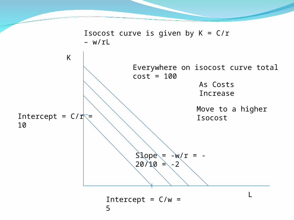
Intercept = C/r = 10

Intercept = C/w = 5

Slope = -w/r = -20/10 = -2

Everywhere on isocost curve total cost = 100

Isocost curve is given by K = C/r – w/rL

As Costs Increase

Move to a higher Isocost

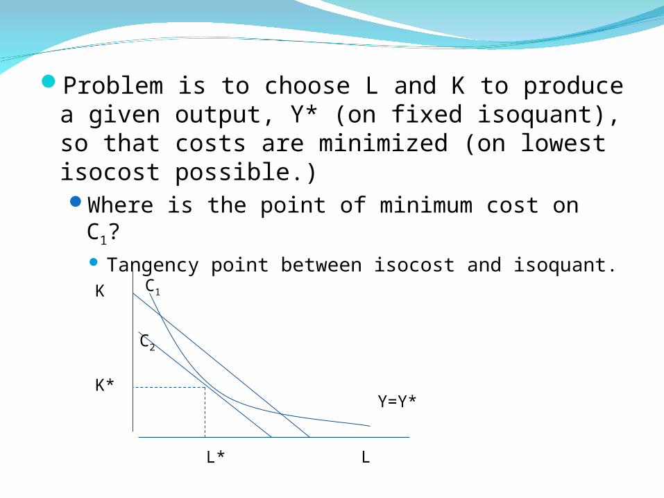
Problem is to choose L and K to produce a given output, Y* (on fixed isoquant), so that costs are minimized (on lowest isocost possible.)Where is the point of minimum cost on C1?

Tangency point between isocost and isoquant.

L

K

Y=Y*

C1

C2

L*

K*

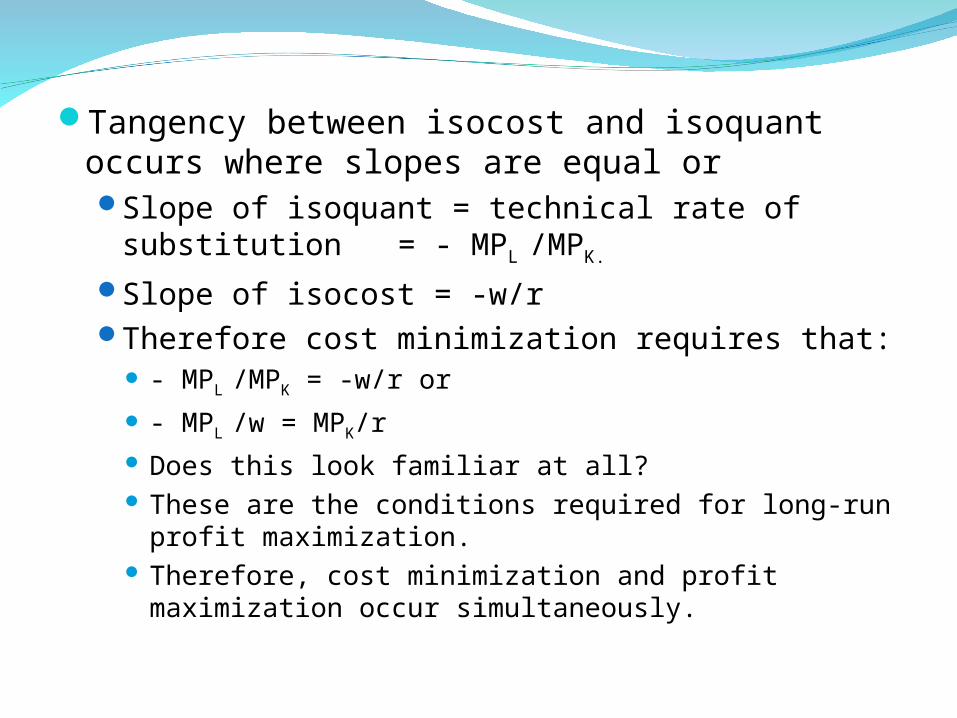
Tangency between isocost and isoquant occurs where slopes are equal orSlope of isoquant = technical rate of

substitution = - MPL /MPK.

Slope of isocost = -w/rTherefore cost minimization requires that:

- MPL /MPK = -w/r or

- MPL /w = MPK/r Does this look familiar at all? These are the conditions required for long-run

profit maximization. Therefore, cost minimization and profit

maximization occur simultaneously.

Let L* and K* define optimal (cost minimizing) L and KL* = f(Y*, w, r)K* = f(Y*, w, r)These are the conditional or derived factor

demand curves.Derived from what?How are profit maximization and cost

minimization different? If maximizing profit => must also be minimizing

costs. If minimizing costs are you necessarily maximizing

profit? No. Why not?

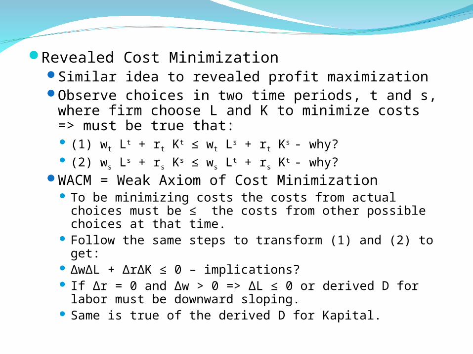
Revealed Cost MinimizationSimilar idea to revealed profit maximizationObserve choices in two time periods, t and s,

where firm choose L and K to minimize costs => must be true that: (1) wt Lt + rt Kt ≤ wt Ls + rt Ks - why? (2) ws Ls + rs Ks ≤ ws Lt + rs Kt - why?

WACM = Weak Axiom of Cost Minimization To be minimizing costs the costs from actual choices

must be ≤ the costs from other possible choices at that time.

Follow the same steps to transform (1) and (2) to get: ΔwΔL + ΔrΔK ≤ 0 – implications? If Δr = 0 and Δw > 0 => ΔL ≤ 0 or derived D for labor

must be downward sloping. Same is true of the derived D for Kapital.

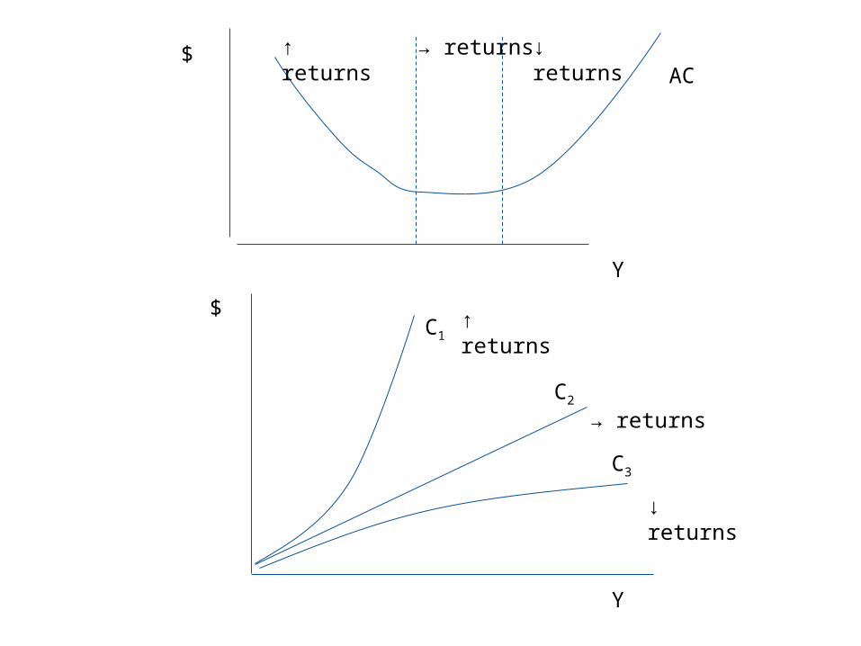
Returns to Scale and Cost FunctionsDefine Average Costs = AC = (C(w, r, Y*))/Y* or:AC = C(Y*)/Y* - (assuming w and r are constant).AC and returns to scale

Constant Returns to Scale AC is constant as Y increases

Increasing Returns to Scale AC is decreasing as Y increases

Decreasing Returns to Scale AC is increasing as Y increases

Why? What does the AC and C look like with the three types

of returns to scale?

Y

$AC

→ returns↑ returns ↓ returns

C1

C2

C3

Y

$ ↑ returns

→ returns

↓ returns

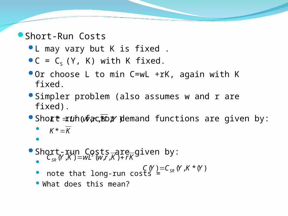
Short-Run CostsL may vary but K is fixed .C = CS (Y, K) with K fixed.Or choose L to min C=wL +rK, again with K fixed.Simpler problem (also assumes w and r are fixed).Short run factor demand functions are given by:

Short-run Costs are given by: note that long-run costs = What does this mean?

),,,(* YKrwLL S

KK *

KrKrwwLKYC SSR ),,(),(

))(*,()( YKYCYC SR

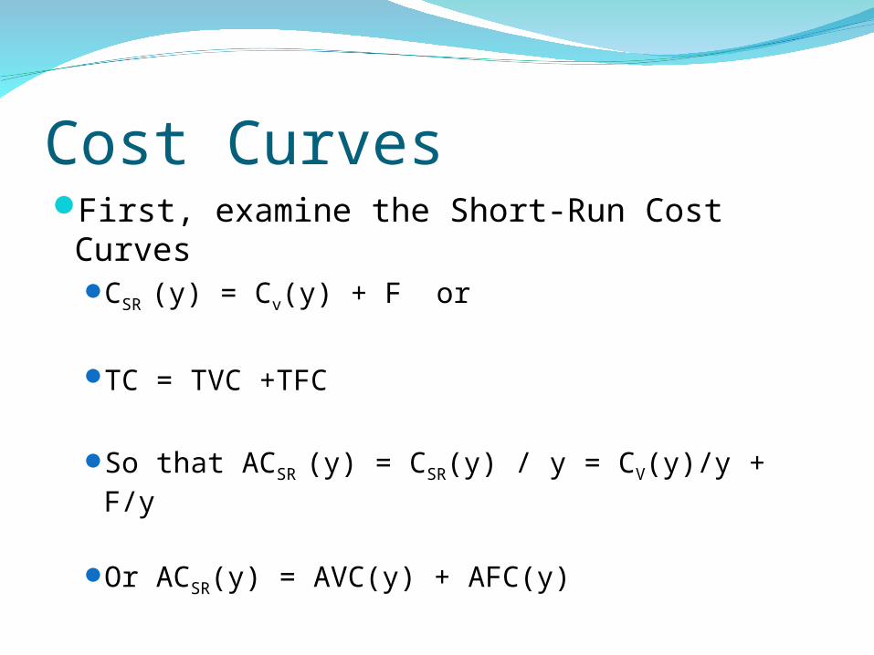
Cost CurvesFirst, examine the Short-Run Cost Curves

CSR (y) = Cv(y) + F or

TC = TVC +TFC

So that ACSR (y) = CSR(y) / y = CV(y)/y + F/y

Or ACSR(y) = AVC(y) + AFC(y)

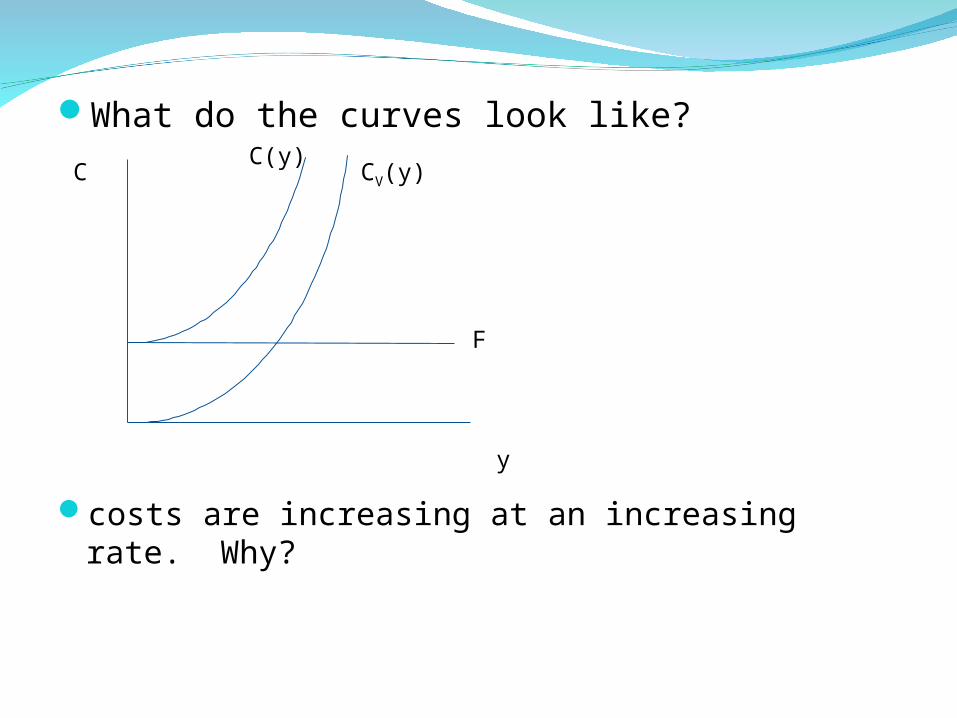
What do the curves look like?

costs are increasing at an increasing rate. Why?

CV(y)C(y)

F

C

y

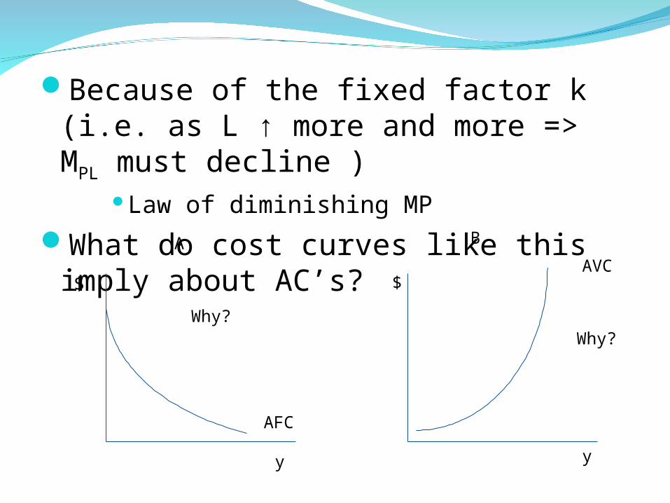
Because of the fixed factor k (i.e. as L ↑ more and more => MPL must decline )

Law of diminishing MPWhat do cost curves like this imply

about AC’s?

AFC

$

y

Why?

AVC$

y

Why?

A B

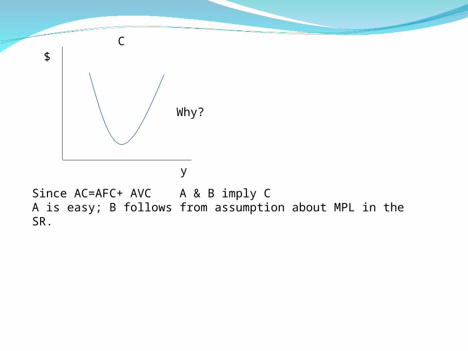
C

Why?

$

y

Since AC=AFC+ AVC A & B imply CA is easy; B follows from assumption about MPL in the SR.

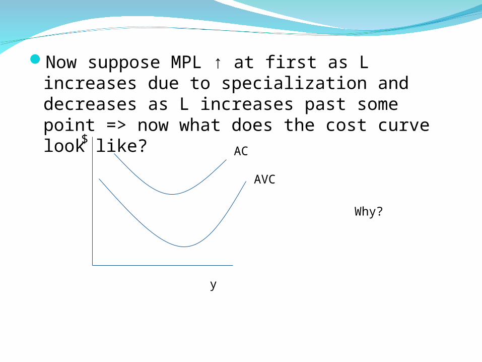
Now suppose MPL ↑ at first as L increases due to specialization and decreases as L increases past some point => now what does the cost curve look like?

$

y

AC

AVC

Why?

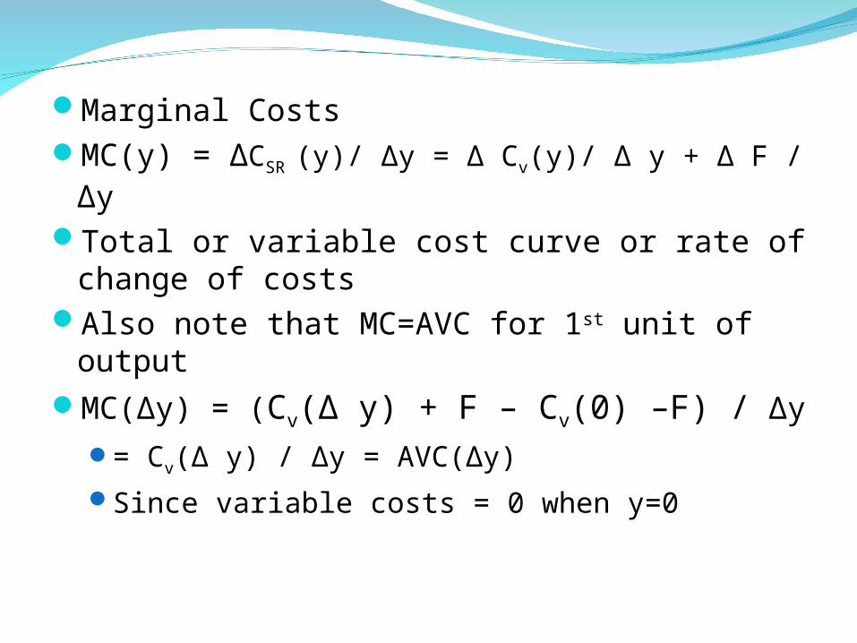
Marginal CostsMC(y) = ΔCSR (y)/ Δy = Δ Cv(y)/ Δ y + Δ F / ΔyTotal or variable cost curve or rate of change

of costsAlso note that MC=AVC for 1st unit of outputMC(∆y) = (Cv(Δ y) + F – Cv(0) –F) / Δy

= Cv(Δ y) / Δy = AVC(Δy)Since variable costs = 0 when y=0

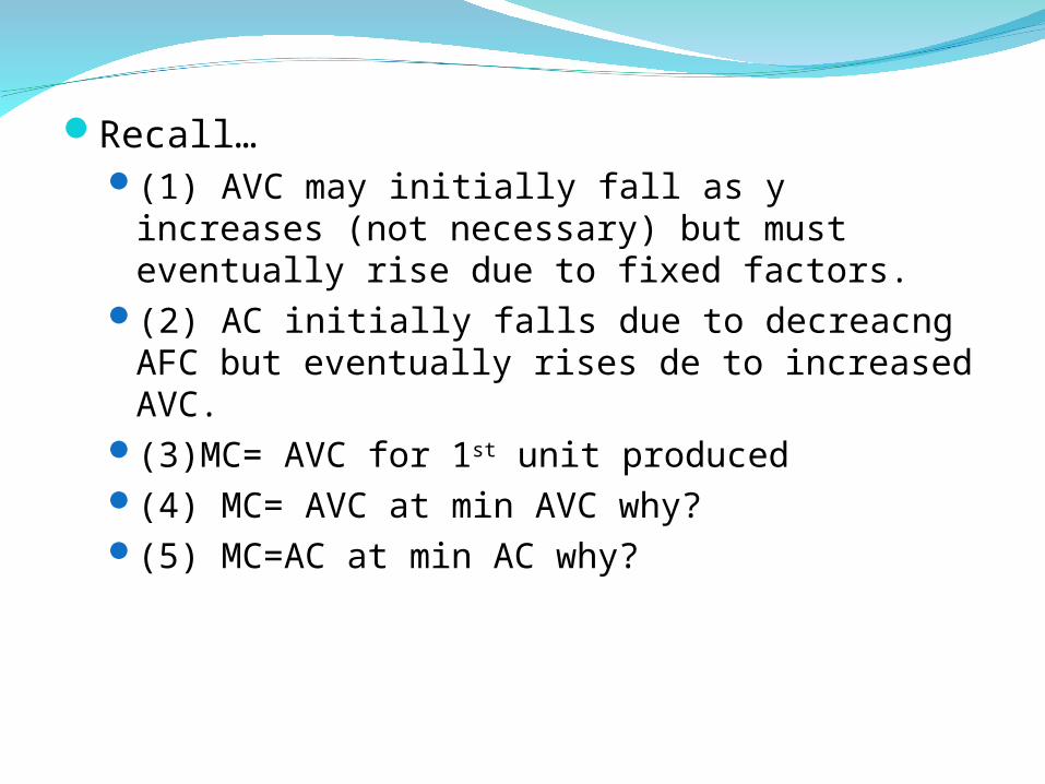
Recall…(1) AVC may initially fall as y increases (not

necessary) but must eventually rise due to fixed factors.

(2) AC initially falls due to decreacng AFC but eventually rises de to increased AVC.

(3)MC= AVC for 1st unit produced(4) MC= AVC at min AVC why?(5) MC=AC at min AC why?

MC

AVC

AC

MC

Y*

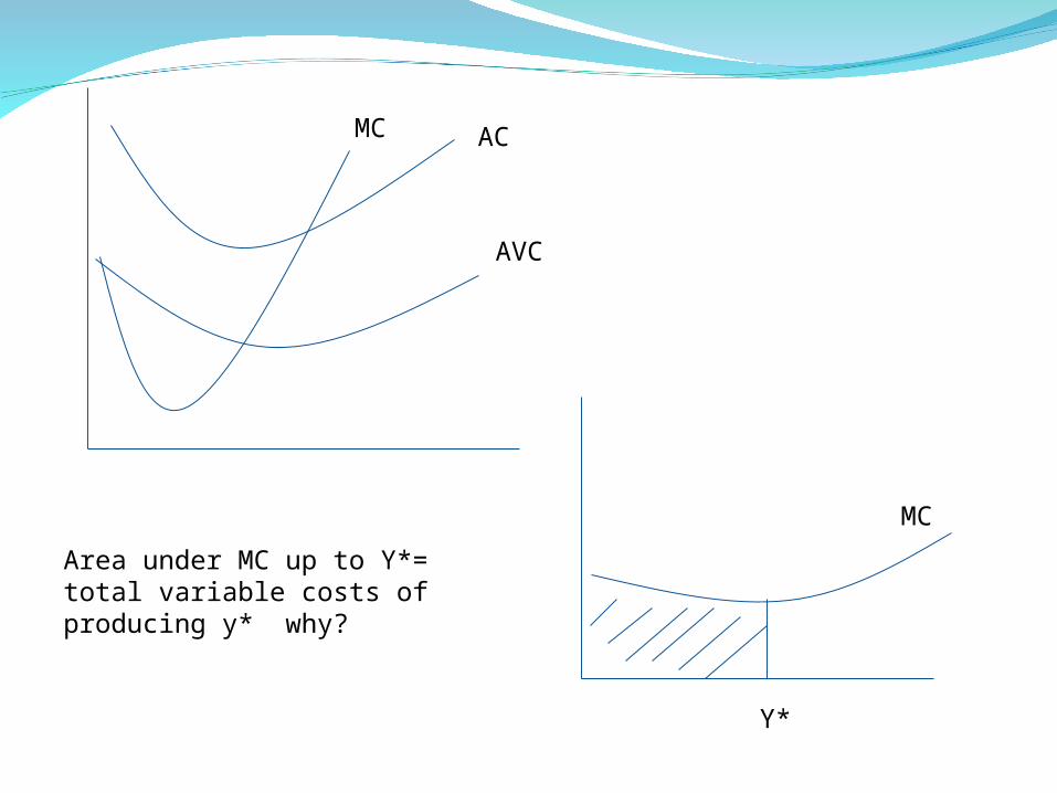
Area under MC up to Y*= total variable costs of producing y* why?

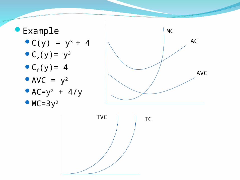
ExampleC(y) = y3 + 4Cv(y)= y3

Cf(y)= 4AVC = y2

AC=y2 + 4/yMC=3y2

MC

AVC

AC

TCTVC

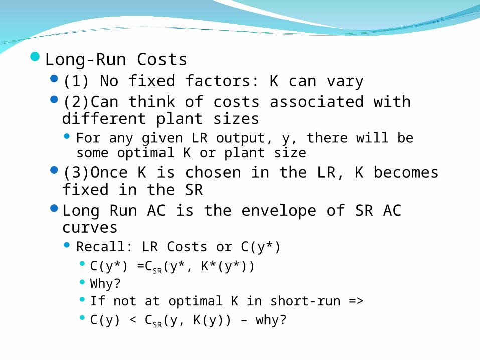
Long-Run Costs(1) No fixed factors: K can vary(2)Can think of costs associated with different

plant sizes For any given LR output, y, there will be some

optimal K or plant size(3)Once K is chosen in the LR, K becomes fixed

in the SRLong Run AC is the envelope of SR AC curves

Recall: LR Costs or C(y*) C(y*) =CSR(y*, K*(y*)) Why? If not at optimal K in short-run => C(y) < CSR(y, K(y)) – why?

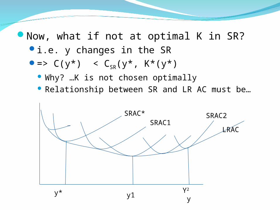
Now, what if not at optimal K in SR?i.e. y changes in the SR=> C(y*) < CSR(y*, K*(y*)

Why? …K is not chosen optimally Relationship between SR and LR AC must be…

y* y1Y2 y

SRAC*SRAC1

SRAC2

LRAC

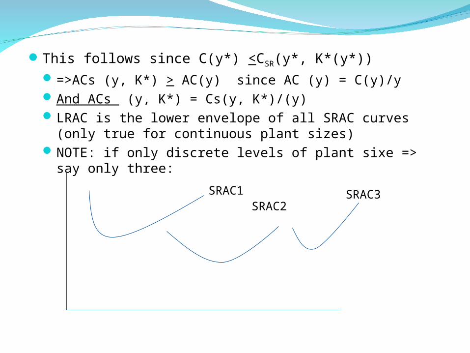
This follows since C(y*) <CSR(y*, K*(y*))=>ACs (y, K*) > AC(y) since AC (y) = C(y)/yAnd ACs (y, K*) = Cs(y, K*)/(y)LRAC is the lower envelope of all SRAC curves (only true

for continuous plant sizes)NOTE: if only discrete levels of plant sixe => say only

three:

SRAC1SRAC2

SRAC3

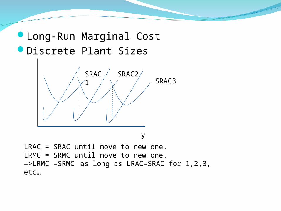
Long-Run Marginal CostDiscrete Plant Sizes

LRAC = SRAC until move to new one.LRMC = SRMC until move to new one.=>LRMC =SRMC as long as LRAC=SRAC for 1,2,3, etc…

SRAC1

SRAC2SRAC3

y

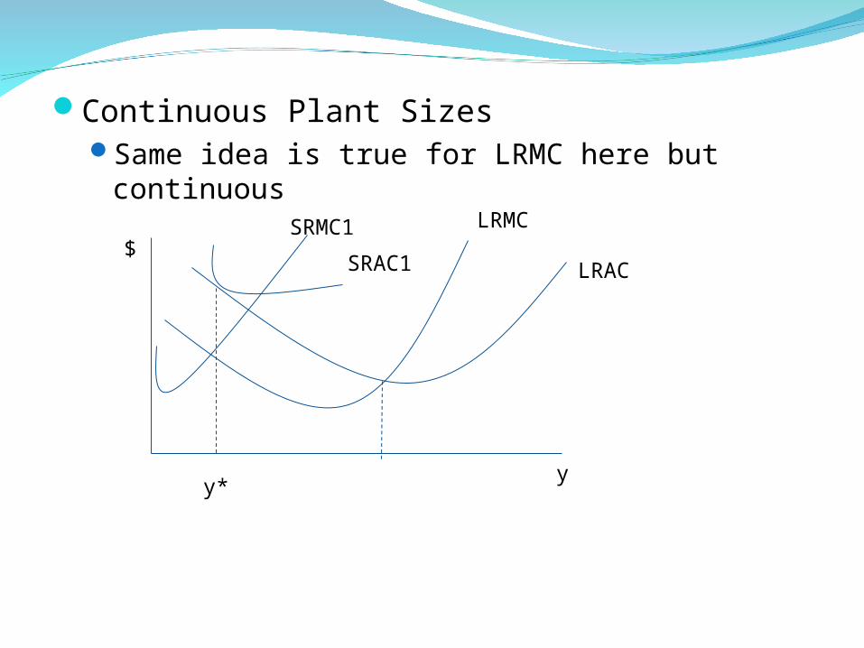
Continuous Plant SizesSame idea is true for LRMC here but

continuous

$LRAC

LRMC

SRAC1

SRMC1

yy*