153

Lecture 7: Minimization or maximization of functions (Recipes Chapter 10)

• Actively studied subject for several reasons:– Commonly encountered problem: e.g. Hamilton’s and

Lagrange’s principles, economics problems, statistical fitting of data (χ2 or maximum likelihood)….

– For the most interesting cases (multivariant, non-linear functions), there is no “best technique”

– There are many competing methods each with some advantages and disadvantages

154

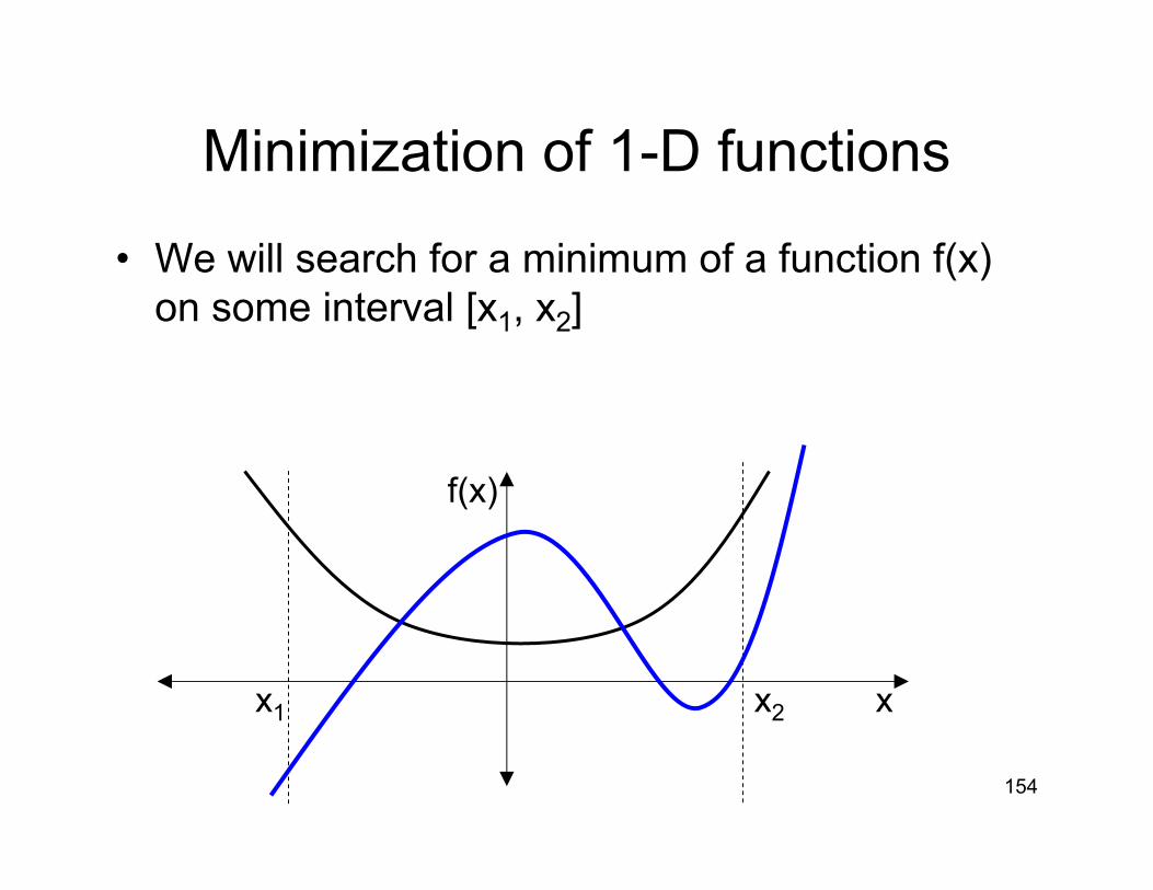
Minimization of 1-D functions

• We will search for a minimum of a function f(x) on some interval [x1, x2]

f(x)

xx1 x2

155

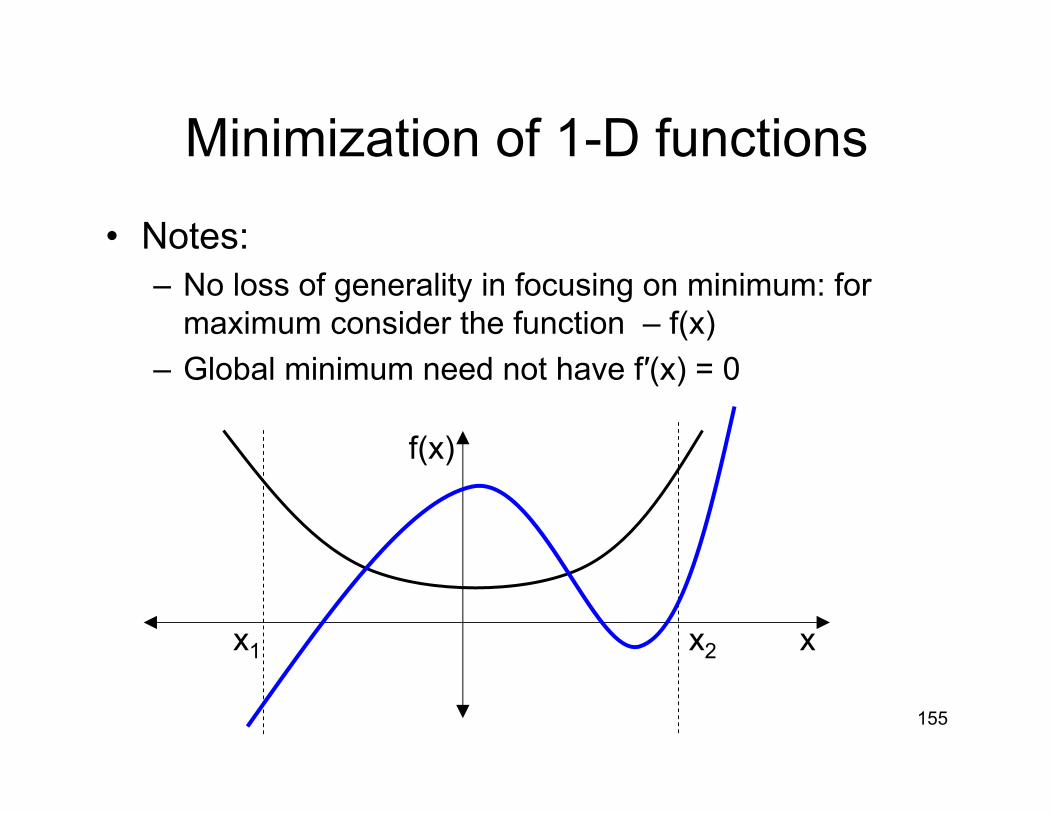
Minimization of 1-D functions

• Notes:– No loss of generality in focusing on minimum: for

maximum consider the function – f(x)– Global minimum need not have f′(x) = 0

f(x)

xx1 x2

156

How accurately can the minimum be found?

• Suppose a minimum of f(x) occurs at x = b (in the case where f′(b) = 0)f(x) = f(b) + f′(b) (x–b) + ½ f′′(b) (x–b)2 + ….

Define δf = f(x) – f(b) as the smallest difference in FP numbers that we can distinguish:Then δf = ε f(b) with ε ~ 10–8 in single precision or ~ 10–16 in double precision

157

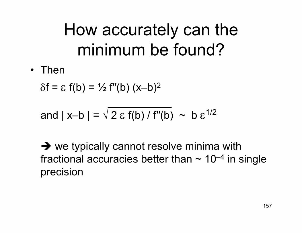
How accurately can the minimum be found?

• Then δf = ε f(b) = ½ f′′(b) (x–b)2

and | x–b | = √ 2 ε f(b) / f′′(b) ~ b ε1/2

we typically cannot resolve minima with fractional accuracies better than ~ 10–4 in single precision

158

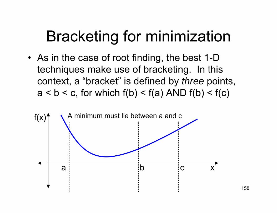
Bracketing for minimization• As in the case of root finding, the best 1-D

techniques make use of bracketing. In this context, a “bracket” is defined by three points, a < b < c, for which f(b) < f(a) AND f(b) < f(c)

f(x)

xa b c

A minimum must lie between a and c

159

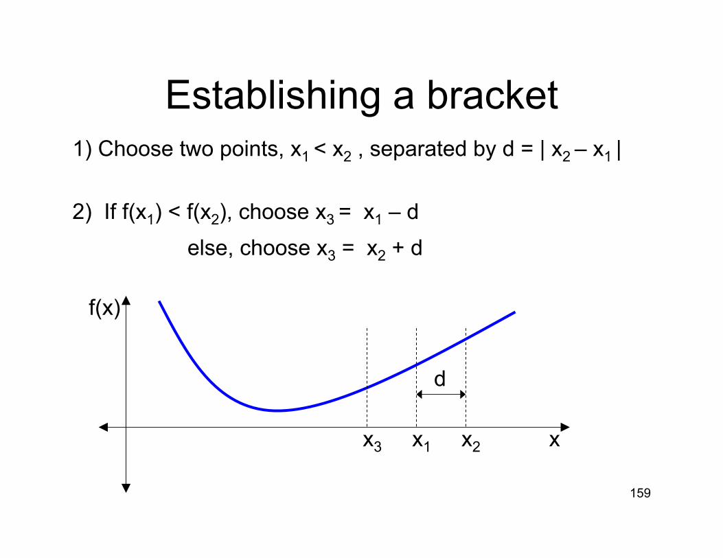
Establishing a bracket1) Choose two points, x1 < x2 , separated by d = | x2 – x1 |

2) If f(x1) < f(x2), choose x3 = x1 – delse, choose x3 = x2 + d

f(x)

xx2x1

d

x3

160

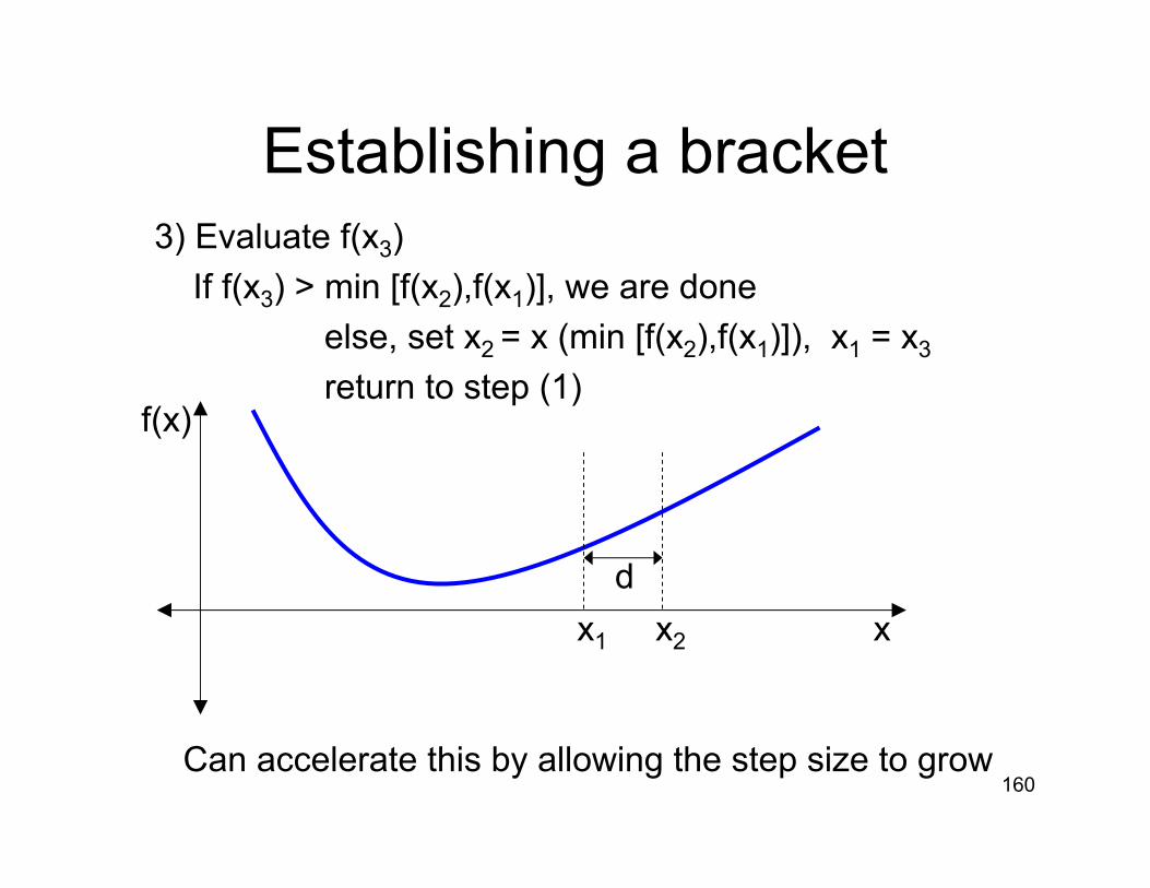
Establishing a bracket3) Evaluate f(x3)

If f(x3) > min [f(x2),f(x1)], we are doneelse, set x2 = x (min [f(x2),f(x1)]), x1 = x3

return to step (1) f(x)

xx2

dx1

Can accelerate this by allowing the step size to grow

161

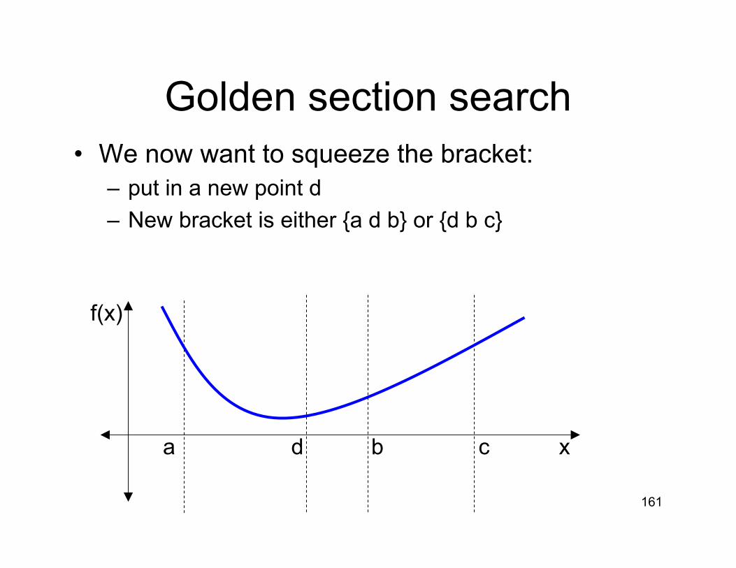
Golden section search• We now want to squeeze the bracket:

– put in a new point d– New bracket is either {a d b} or {d b c}

f(x)

xa b cd

162

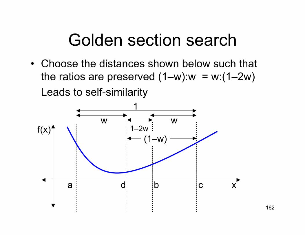
Golden section search• Choose the distances shown below such that

the ratios are preserved (1–w):w = w:(1–2w)Leads to self-similarity

f(x)

xa b cd

1w w

1–2w(1–w)

163

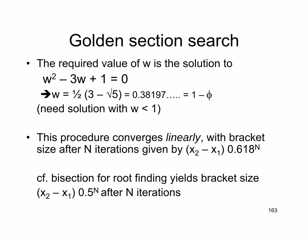
Golden section search• The required value of w is the solution to

w2 – 3w + 1 = 0 w = ½ (3 – √5) = 0.38197….. = 1 – φ

(need solution with w < 1)

• This procedure converges linearly, with bracket size after N iterations given by (x2 – x1) 0.618N

cf. bisection for root finding yields bracket size (x2 – x1) 0.5N after N iterations

164

Faster methods• As with bisection, in the Golden section

method we only ask about whether certain quantities (e.g. f(d) – f(c) are positive of negative)

• We can accelerate convergence by using more information about the values of various quantities

165

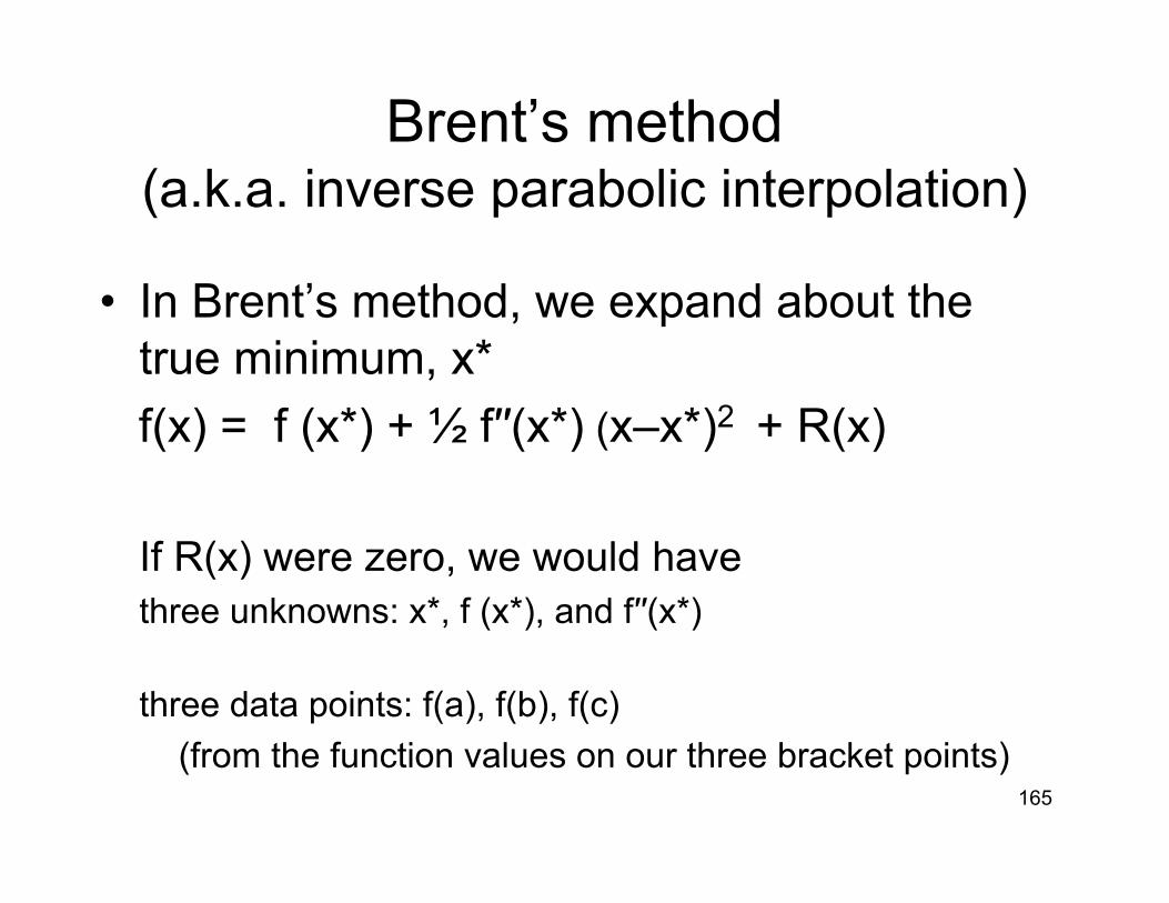
Brent’s method(a.k.a. inverse parabolic interpolation)

• In Brent’s method, we expand about the true minimum, x*f(x) = f (x*) + ½ f′′(x*) (x–x*)2 + R(x)

If R(x) were zero, we would have three unknowns: x*, f (x*), and f′′(x*)

three data points: f(a), f(b), f(c) (from the function values on our three bracket points)

166

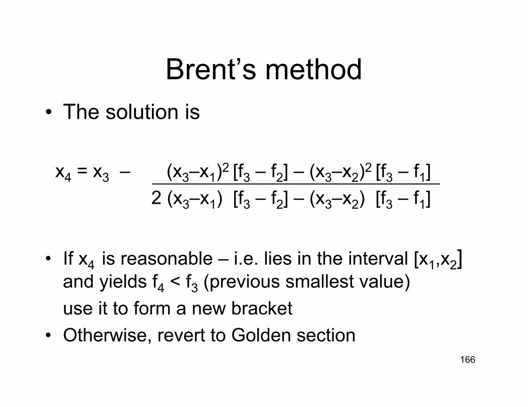
Brent’s method• The solution is

x4 = x3 – (x3–x1)2 [f3 – f2] – (x3–x2)2 [f3 – f1] 2 (x3–x1) [f3 – f2] – (x3–x2) [f3 – f1]

• If x4 is reasonable – i.e. lies in the interval [x1,x2] and yields f4 < f3 (previous smallest value)use it to form a new bracket

• Otherwise, revert to Golden section

167

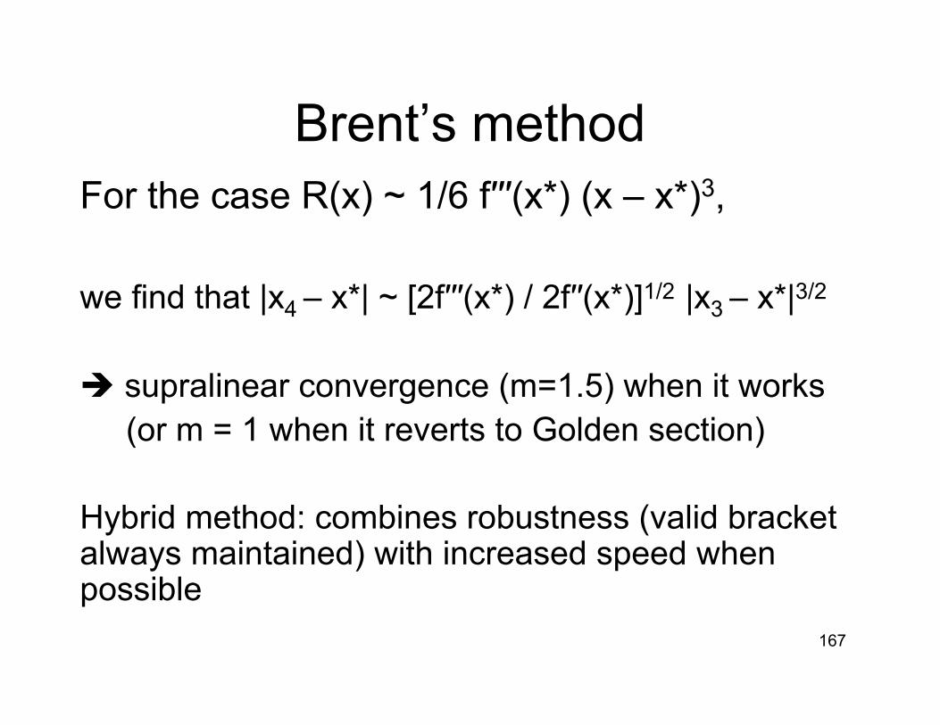
Brent’s methodFor the case R(x) ~ 1/6 f′′′(x*) (x – x*)3,

we find that |x4 – x*| ~ [2f′′′(x*) / 2f′′(x*)]1/2 |x3 – x*|3/2

supralinear convergence (m=1.5) when it works(or m = 1 when it reverts to Golden section)

Hybrid method: combines robustness (valid bracket always maintained) with increased speed when possible

168

Use of derivative information

• When f′(x) is known explicitly, this information can be used to further improve performance– Recipes has a hybrid routine that uses the

secant method to find the root of f′(x) with the Golden section method to ensure that a bracket is maintained

169

Multi-D minimization (Numerical Recipes, §10.4 – 10.7)

• As with root finding, things get a lot harder when f is a function of several variables– no analog to a “bracket”

• Overview of techniques– Function evaluations only downhill simplex method– Function evaluation to estimate the optimum direction

of motion Powell’s method– Function evaluations and explicit gradient calculation

Conjugate Gradient Method

170

Downhill simplex

• A simplex is a hyperpolygon of N + 1 vertices in an N-dimensional space

N = 2: triangleN = 3: tetrahedron

• If one vertex is at the origin of the coordinate system, the others are given by N vectors which span the N-dimensional space:Vi = Pi – P0 (i = 1, N), where Pi is the ith vertex

171

Downhill simplex

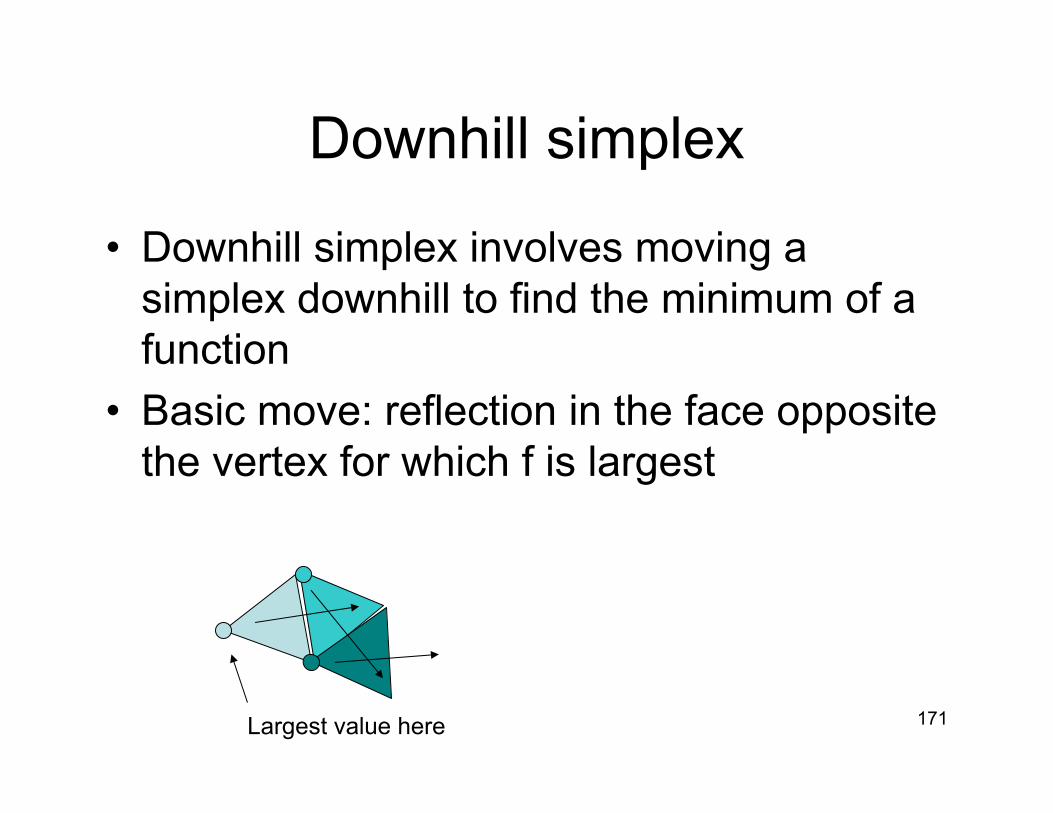
• Downhill simplex involves moving a simplex downhill to find the minimum of a function

• Basic move: reflection in the face opposite the vertex for which f is largest

Largest value here

172

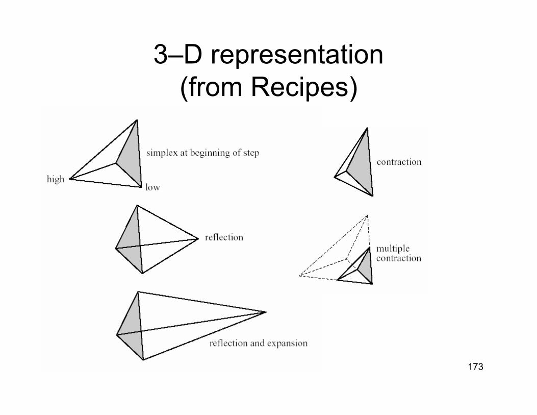
Downhill simplex

• Additional moves:– Stretch to accelerate motion in a

particular direction– Contraction, if reflection overshoots the

minimum • Press et al. name their routine AMOEBA

173

3–D representation (from Recipes)

174

Direction set methods

• Basic tool of all such methods is a 1-D minimization (Golden section, Brent’s method)

• Choose a starting position p, and a direction n, and minimize f (p+λn)

• Now use p+λn as the new starting position, choose a different direction, and minimize along that direction…….

• Methods differ as to how the directions are chosen

175

Direction set methods

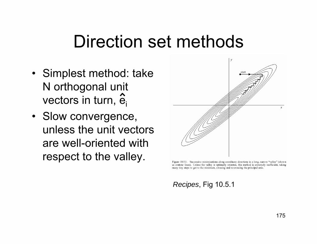
• Simplest method: take N orthogonal unit vectors in turn, ei

• Slow convergence, unless the unit vectors are well-oriented with respect to the valley.

Recipes, Fig 10.5.1

176

Direction set methods

• Better methods update the directions as the method proceeds, so as to– choose favorable directions that proceed far

along narrow valleys– choose “non-interfering” directions, such that

the next direction doesn’t undo the minimization achieved by previous steps

177

Steepest descent

• If you know the derivatives of f (i.e. you know ∇f), you might think that you would do best to choose n = – ∇f / |∇f|

• This is the method of steepest descent• BUT, this means you always choose a

new direction that is orthogonal to the previous directioni.e. ni+1 . ni = 0

178

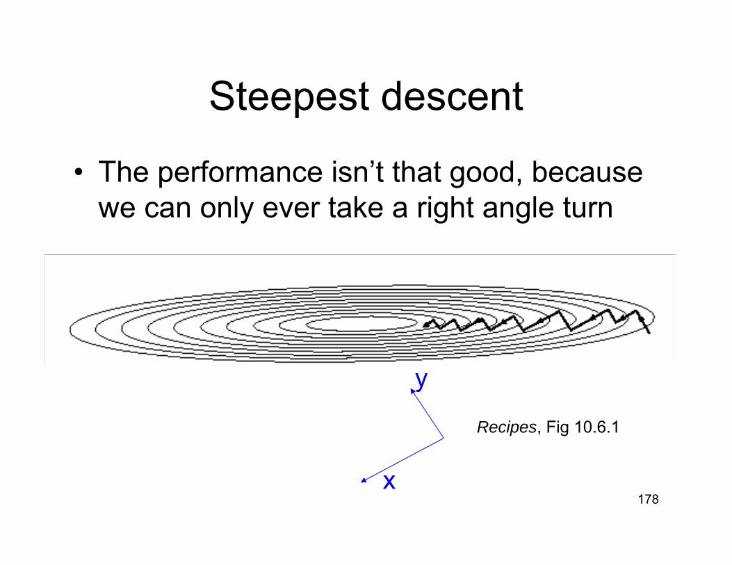
Steepest descent

• The performance isn’t that good, because we can only ever take a right angle turn

Recipes, Fig 10.6.1

x

y

179

Steepest descent: 2-D example• Suppose step k occurred along the y-axis, and led to

position pk+1, at which ∂f/∂y = 0.

• Next step is along the x-axis: that step leads to a position pk+2 , where ∂f/∂x = 0

• But if ∂2f /∂y∂x is non-zero, ∂f/∂y will no longer be zero.

• We really want to move along some direction other than the x-axis, such that ∂f/∂y remains zero.