
JETC IX - Accueil · Michel COURNIL, Ecole des mines, ... Antonio VALERO, Saragosse ... Joint...
240
JETC IX Joint European Thermodynamics Conference IX Ecole nationale supérieure des mines de Saint-Etienne, June 12-15 2007 Proceedings Editors : Bernard Guy and Daniel Tondeur Chaleur Heat Calor Wärme Varme Calore Θερμότητα חום
Transcript of JETC IX - Accueil · Michel COURNIL, Ecole des mines, ... Antonio VALERO, Saragosse ... Joint...
JETC IX
Joint European Thermodynamics Conference IX
Ecole nationale supérieure des mines de Saint-Etienne, June 12-15 2007
Proceedings
Editors : Bernard Guy and Daniel Tondeur
Chaleur
Heat
Calor
Wärme
Varme Calore
Θερμότητα
חום

JETC IX – 12-15 June 2007 Joint European Thermodynamics Conference IX
Ecole nationale supérieure des mines de Saint-Étienne, France
Contents
Foreword....................................................................................................................................1 Committees................................................................................................................................2 Acknowledgements ...................................................................................................................3 Program .....................................................................................................................................4 The Ilya Prigogine prize of thermodynamics ..........................................................................13 List of papers (alphabetic order of the first authors) ...............................................................15 List and numbers of posters...................................................................................................219 Geological field trip...............................................................................................................221 Exhibition on thermodynamics..............................................................................................223 Exhibition of old and rare books on thermodynamics...........................................................225 Ceilidh ...................................................................................................................................227 Ecast ......................................................................................................................................228 List of authors........................................................................................................................229

JETC IX – 12-15 June 2007 Joint European Thermodynamics Conference IX
Ecole nationale supérieure des mines de Saint-Étienne, France
1
Foreword
Why organize a conference on thermodynamics ? Are the bases of the discipline not founded solidly enough? And are the applications now so various that the dialog between the specialists from chemistry, geology, materials science, chemical engineering etc., all using thermodynamics in their own way, is becoming impossible? As a matter of fact, thermodynamics is continuously developing and new ideas and methods do appear at all levels (concepts, scale changes, mesoscopic thermodynamics and links with the nano-sciences, ab-initio methods, optimisation etc.). For this reason, it is important that all the scientists that use it and make it progress can find a place to exchange and promote new ideas. Some new methods in a domain may also appear be useful in another. So the first aim of the conference is to make a review of current research in thermodynamics and promote interdisciplinary exchanges on the progresses of thermodynamics; the focus will be given on the concepts and on the methods rather than on the applications, or in that case mostly provided a general bearing may be given. Welcome to Saint-Etienne! Pourquoi un congrès de thermodynamique? Les bases de la discipline ne sont-elles pas fondées solidement ? Et ses applications ne sont-elles pas maintenant si dispersées que le dialogue entre les spécialistes qui l’utilisent dans des domaines aussi éloignés que la chimie, la géologie, les matériaux, le génie des procédés etc. est devenu impossible ? Non, il se trouve que la thermodynamique connaît sans cesse de nouveaux développements à tous les niveaux (concepts, changements d’échelle, thermodynamique mésoscopique et liens avec les nano-sciences, méthodes ab initio, optimisation etc.). Et, pour cette raison, il est important que tous ceux qui l’utilisent et la font progresser puissent trouver un lieu pour échanger et promouvoir de nouvelles idées : de nouvelles méthodes dans un domaine peuvent-elles servir dans un autre ? Telle est l’ambition première de ce congrès : faire le point, être un lieu d’échange pluri- et inter-disciplinaire sur les progrès de la thermodynamique, en se focalisant sur les concepts et les méthodes plus que les applications. Bienvenue à Saint-Etienne ! Bernard GUY and Daniel TONDEUR, chairs of the scientific committee of JETC IX
JETC IX – 12-15 June 2007 Joint European Thermodynamics Conference IX
Ecole nationale supérieure des mines de Saint-Étienne, France
2
Committees
Scientific committee Bernard GUY, Ecole des mines, Saint-Etienne and Daniel TONDEUR, Ensic, Nancy chairs of the scientific committee Bjarne ANDRESEN, Niels Bohr Institute, Copenhagen Dick BEDEAUX, Leyden José CASAS-VASQUEZ, University of Barcelona Danièle CLAUSSE, UTC, Compiègne Michel COURNIL, Ecole des mines, Saint-Etienne Alexis De VOS, University of Gent Jean-Pierre DUMAS, University of Pau Jean DUBESSY, CNRS, Nancy Daniel FARGUE, Ecole des mines, Paris Walter FURST, ENSTA, Paris Daniel GARCIA, Ecole des mines, Saint-Etienne Karl-Heinz HOFFMANN, Chemnitz Christian JALLUT, CPE, Lyon François MARECHAL, Ecole polytechnique fédérale de Lausanne Jean-Karl PLATTEN, University of Mons Dominique RICHON, Ecole des mines de Paris, Fontainebleau Jacques ROUX, CNRS, Paris Michel SOUSTELLE, Ecole des mines, Saint-Etienne Annie STEINCHEN-SANFELD Marseille Antonio VALERO, Saragosse
Local organization committee Bernard GUY, Ecole des mines, Saint-Etienne Grégoire BERTHEZENE, Ecole des mines (website) Gérard THOMAS, Ecole des mines Olivier BONNEFOY, Ecole des mines Jean-Luc BOUCHARDON, Ecole des mines Emilie POURCHEZ, Ecole des mines (exhibition on thermodynamics) Joëlle VERNEY, Ecole des mines (secretary) Frédéric GALLICE, Ecole des mines
Organisation of geological field trip Bernard GUY, Ecole des mines Jean-Yves COTTIN, Université Jean Monnet, Saint-Etienne Jean-Luc BOUCHARDON, Ecole des mines

JETC IX – 12-15 June 2007 Joint European Thermodynamics Conference IX
Ecole nationale supérieure des mines de Saint-Étienne, France
3
Acknowledgements We thank the following people : Frédrérique Arcos from Tourist Office for her help in the hotel and gala organisation, Marine Triomphe from Ecole des mines and BV Conseil for their help in the public relations of the conference, Noël Paul from Saint-Etienne Métropole for funding the conference, M. Michel Thiollière, Mayor of Saint-Etienne for welcoming us in the Town-Hall and Mrs Fontanilles and Tavernier for their help, All the members of the committees (refer to page 2), especially Joëlle Verney and Grégoire Berthezène; and also all those who helped us in so many ways and do not apprear in the previous lists: the doctorate researchers: Frédéric Bard, Franck Diedro, Morad Lakhssassi and Guillaume Battaia; Marc Doumas and Jacques Moutte (Ecole des mines) ; Marie-Christine Gerbe and Peter Bowden (university of Saint-Etiennne), and all the people in Ecole des mines who worked for the organisation tasks… Our non-thermodynamicists wifes and husbands…

JETC IX – 12-15 June 2007 Joint European Thermodynamics Conference IX
Ecole nationale supérieure des mines de Saint-Étienne, France
4
Program
Joint European Thermodynamics Conference IX, JETC IX
Ecole nationale supérieure des mines de Saint-Etienne
Saint-Etienne, France
12-15 June 2007
This program may still be modified… Please tell us if there is a big discrepancy with your schedule or if there are mistakes. 65 communications: 40 oral communications and 25 poster communications. The oral communications last for 20 minutes including discussion (prepare 15 minutes talks) and the oral presentations of posters last for 3 minutes (no discussion, prepare 3 slides). Please bring your ppt file in advance, i.e. before the session, to the computer in the main amphitheatre. Those participants who have written books are invited to bring copies along with them for display during the conference Posters come first! Start your day by a look at the posters between 8h 30 and 9h 30 each day! Four main themes : A. Foundations of thermodynamics : history, philosophy, teaching of thermodynamics, I. Prigogine’s legacy, new approaches B. Non-equilibrium thermodynamics: thermodiffusion, kinetics of phase transitions, transport processes, advanced concepts C. Equilibrium thermodynamics: equations of state, phase equilibria, nanosystems, computation D. Optimization and engineering systems: exergy, energy, finite-time thermodynamics
JETC IX – 12-15 June 2007 Joint European Thermodynamics Conference IX
Ecole nationale supérieure des mines de Saint-Étienne, France
5
Day 1: Tuesday June 12 2007 8h 30 - 9h 30: registration, installation of posters, coffee, a first look to the exhibitions (thermodynamics, books) 9h 30 – 10h 50: Welcome and session A1 - 20 minutes, chair B. Guy: - welcome addresses: Bernard Guy, Daniel Tondeur, Jean-Charles Pinoli (Ecole des mines), Noël Paul (Saint-Etienne Métropole) - announcements: exhibition on thermodynamics: Emilie Pourchez, and Ecole des mines students; exhibition on books: Thierry Veyron; Ceilidh: Peter Bowden; publication of presentations in thermodynamics journals: Daniel Tondeur ; geological excursion: B. Guy - 60 minutes: Session A1 : 3 oral communications; chair: D. Tondeur • Gian Paolo Beretta : Axiomatic definition of entropy for non-equilibrium states • Jean-François LeMaréchal: Teaching and learning thermodynamics at school • Bernard Guy: Prigogine and the time problem 10h 50 - 11h 20: coffee break 11h 20 –12h 40: Session B1: 4 oral communications; chair: J. Casas Vasquez • Simone Wiegand et al.: Thermal diffusion of neutral and charged colloidal dipersions • I. Ryzhkov et al.: On thermal diffusion and convection in multicomponent mixtures with application to thermogravitational column • J. Xu et al.: Transport properties of a reactive mixture in a temperature gradient a studied by molecular dynamics simulations • P. Galenko et D. Jou: Diffuse interface model for non-equilibrium phase transformations 13h - 14h 30: lunch 14h 30 –15h 50: Ilya Prigogine prize of thermodynamics and Session B2: chair: B. Andresen 40 minutes: Ilya Prigogine prize of thermodynamics • Stefano Mazzoni: Pattern formation in convective instabilities in a colloidal suspension 40 minutes: Session B2: 2 oral communications, chair: B. Andresen (continued) • E. Nourtier Mazauric et al.: A kinetic model for describing reactions between ideal solid solutions and aqueous solutions • F. Girard et al.: Influence of heating substrate geometry and humidiy on the dynamics of evaporating sessile water droplets 15h 50 –16h 20: Coffee break
JETC IX – 12-15 June 2007 Joint European Thermodynamics Conference IX
Ecole nationale supérieure des mines de Saint-Étienne, France
6
16h 20- 17h 40: Session B3 and Presentation of posters 1 - 40 minutes: Session B3: 2 communications; chair: A. de Vos • W. Wolczynski: Criterion of minimum entropy production applied to the explanation of lamella/rod transformation • Michel Pons : The transition from single- to multi-cell natural convection of air in cavities with an aspect ratio of 20 - 40 minutes: presentation of posters 1: 14 posters (themes C and A); chair: K.H. Hoffmann 1.• C. Giraldo et al.: Ethane gaz hydrate incipient conditions in reversed micelles 2 • D. Vasilyev and A. Udovsky: Interconsistency between three types of diagrams for calculation of optimized thermodynamic properties of alloys of the U-Zr system 3 • JF Dalloz: New equations of state for various gases (Ar, CO2, C2 H2 , C2H4, NH3, N2, O2) obtained from experimental data 4 • A. Abbaci and A. Acidi: Supercritical fluids: case of hexane 5 • A. Bougrine et al.: Determination of liquid/vapour equilibria by ebulliometry and modelling by the quasi-ideal model 6 • E. Labarthe et al.: Determination of solid-liquid equilibria in the ternary system piperidine-sodium sulphate water by isoplethic thermic analysis: study of the isothermal sections 293K, 298K, 313K 7 • P. Paricaud et al.: Recent advances in the use of the SAFT approach to describe the phase behaviour of associating molecules, electrolytes and polymers 8 • M. Lakhssassi et al. : A “magmatic isotherm” for the exchange of Fe and M between an olivine solid solution and a melt 9 • A. Udovsky and M Kupavtsev: The development of software for automatic computer program for calculation of two-phase tie-lines and thermodynamic properties of two-phase alloys in closed ternary systems using the natural coordinates 10 • G. Beretta: Non linear generalization of Schrödinger’s equation uniting quantum mechanics and thermodynamics 11 • C. Firat and A Sisman: Quantum surface energy and lateral forces in ideal gases 12 • A Truyol: Thermodynamics and nanosciences and nanotechnologies 13 • F Dennery: Entropy grows whatever the signs of temperature and time in their arrows 14 • P. Galenko and V. Lebedev: Local non-equilibrium effect on spinodal decomposition in a binary system End of afternoon: 18h 30: reception at the Mairie de Saint-Etienne: remittance of the Ilya Prigogine Prize of Thermodynamics to Stefano Mazzoni in presence of the Mayor of Saint-Etienne, Michel Thiollière To go to the Town Hall (Mairie), you may take bus n° 6 and walk (15 minutes), or walk the whole way (30 minutes).
JETC IX – 12-15 June 2007 Joint European Thermodynamics Conference IX
Ecole nationale supérieure des mines de Saint-Étienne, France
7
Day 2, Wednesday June 13, 2007 8h 30 - 9h 30: posters, exhibitions (thermodynamics, books), coffee 9h 30 – 10h 50: Session D and presentation of posters 2 Session D (3 oral communications); chair D. Tondeur • Karl Heinz Hoffmann: Quantifying dissipative processes • M. Sorin F. Rheault and B. Spinner: Thermodynamically guided modelling and intensification of steady state processes (cancelled) • JF Portha et al.: Application of exergy analysis and life cycle assessment to naphta catalytic reforming • V. Shevtsova and A. Mialdun: Measurement of Soret coefficients in aqueous solutions Poster presentation 2 (Theme D): 5 oral presentations, 20 minutes; chair : D. Tondeur 15 • J. Garrido: Thermodynamics of electrodialysis processes 16 • M. Feidt et al.: What’s new with thermodynamic optimization of refrigerating machines, with regards to design and control-command: a review synthesis 17 • M. Nikaien et al.: Thermodynamic optimization of Brayton cycle wih steam engine injection using exergy analysis 18 • M. Serier and A Serier: Evolutions thermodynamics of a driving fluid in a cylinder with valves 19 • M. Radulescu et al.: Hybrid combined heat and power plants using a solid oxide fuel cell and external steam reformer 10h 50 - 11h 20: coffee break 11h 20 –12h 40: Session C1: 4 oral communications; chair A. de Vos • A. Laouir and D. Tondeur: First and second law application to processes involving capillarity • J. Faraudo and F. Bresme: Thermodynamic of nanoparticles at liquid/liquid interfaces • E. Perfetti, J. Dubessy and R. Thiery: An equation of state taking into account hydrogen bonding and diplar interactions: application to the modelling of liquid-vapour phase equilibria (PVTX properties) for H2O - gaz (H2S, CO2, CH4) systems • M. Bendova et al.: Liquid-liquid equilibrium in the binary system 1-butyl – 3 – methylimidazolium hexafluorophosphate + water. Quantitative analysis of the experimental data 13h - 14h 30: lunch
JETC IX – 12-15 June 2007 Joint European Thermodynamics Conference IX
Ecole nationale supérieure des mines de Saint-Étienne, France
8
14h 30 –15h 50: Session C2: 4 communications; chair J. Dubessy • S. Sarraute et al.: Aqueous solubility and partition coefficients of halogenated hydrocarbons as a function of molecular structure • SL Hafsaoui et al.: Prediction of activiy coefficients in non ideal solutions • P. Paricaud et al.: From dimer to condensated phases at extreme conditions: accurate prediction properties of water by a Gaussian charge polarisable model • J. Moutte: The Arxim project: modules for the computation of thermodynamic equilibrium in heterogeneous systems; applications to the simulation of fluid-rock systems 15h 50 –16h 20: Coffee break 16h 20- 17h 40: Session A2: 3 communications, 60 minutes; chair: B. Guy • Pierre Perrot: Some problems in the teaching of thermodynamics • Jakob de Swaan: Waiting for Carnot: thermodynamics concepts and complex processes • François-Xavier Demoures: The controversy between Boltzmann and Ostwald 17h 30: departure to Saint-Victor sur Loire; visit of the village, meal, back to Saint-Etienne at 22h 30.
JETC IX – 12-15 June 2007 Joint European Thermodynamics Conference IX
Ecole nationale supérieure des mines de Saint-Étienne, France
9
Day 3: Thursday June 14 2007 8h 30 - 9h 30: posters, exhibitions (thermodynamics, books) coffee 9h 30 – 10h 50: Session B4, 4 oral communications; chair: J. de Swaan • V. Mendez and J. Casas Vazquez: Hyperbolic reaction diffusion model for virus infection • D. Queiros-Conde and M. Feidt: Entropic skins geometry and dynamics of turbulent reactive fronts • B. Noack et al.: A finite time thermodynamics of unsteady flows from the onset of vortex shedding to developed homogeneous turbulence • D. Clausse et al.: Mass transfer kinetics in O/W/O multiple emulsions 10h 50 - 11h 20: coffee break 11h 20 –12h 40: Session C3 and poster presentation 3, chair: D. Clausse C3: 3 oral communications • Pascal Richet: Thermodynamics of molten silicates: connection with structure and transport properties • B. Sedunov: Monomolecular fraction in real gases • A. Udovsky: The evolution of ideas in the field of analytical and computational thermodynamics of multi-component systems: from J.W. Gibbs up to XXI century Poster presentation 3: 20 minutes, 5 posters (theme B); chair: D. Clausse (continued) 20 • P. Blanco et al.: A predictive phenomenological law of the thermodiffusion coefficient in organic mixtures of n-alkanes nCi- nCj (i, j = 5, …, 18) at 25 ° and 50 wt% 21 • W. Kölher et al.: A systematic study of the Soret coefficient of binary liquid mixtures 22 • A. Zebib: Convective instabilities of ternary mixtures in thermogravitational columns 23 • P. Polyakov: Study of thermal diffusion behaviour of alkane/benzene mixtures by thermal diffusion forced Rayleigh scattering experiments and lattice model calculations 25 • B Guy: Geology and thermodynamics 13h - 14h 30: lunch 14h 30 –15h 50: Session B5: 4 oral communications; chair: D. Richon • B. Andresen and C. Essex: Mitochondrial optimization using thermodynamic geometry • S. Sieniutycz: Constant Hamiltonian paths for power producing relaxation of non-linear resources • F. Couenne et al.: Thermodynamic of irreversible processes: a tool for computer aided dynamic modelling of processes by using bond graph language • A. DeVos: Reversible computers
JETC IX – 12-15 June 2007 Joint European Thermodynamics Conference IX
Ecole nationale supérieure des mines de Saint-Étienne, France
10
15h 50 –16h 20: Coffee break 16h 20- 17h 40: Last Session; chair: P. Richet 2 oral communications • T. Veyron: Before thermodynamics: a short history of the steam engine • Daniel Tondeur: Optimal distribution of irreversibilities in multi-scale fluidic trees End of conference In the evening: Social folk danse (Ceilidh), Villars (5€ charge per person)
JETC IX – 12-15 June 2007 Joint European Thermodynamics Conference IX
Ecole nationale supérieure des mines de Saint-Étienne, France
11
Day 4: Friday June 15 Geological field trip Departure: Saint-Etienne: 8h 30 9h 30 : First stop: Col du Pertuis View point (Le Puy area, Devès etc.) : the different types of volcanic rocks as seen in the landscape (different geomorphologic behavior): basaltic cones and flows, trachyte and phonolithe intrusions… The problem to understand the link between these different rocks in the same area. 10h 30: Second stop: suc de Monac The phonolithic dyke of Monac: inspection of the rock. General view of the outcrop. 11h 30: Third stop: basaltic lava lake of Noustoulet The basaltic rock and its peridotites enclaves. The columnar jointing of basalts. General discussion: - fractionate cristallization of magmas and phase diagrams - partial fusion of peridotites and the formation of basalts - geothermometers and geobarometers and the physical conditions for the formation of enclaves - columnar jointing of basalts: constitution undercooling or thermal induced stress? 13h: Saint-Jullien Chapteuil Lunch 15h : End 16h: Back to Saint-Etienne
JETC IX – 12-15 June 2007 Joint European Thermodynamics Conference IX
Ecole nationale supérieure des mines de Saint-Étienne, France
12
Sessions and chairs
Day 1 Welcome session: B. Guy Session A1: D. Tondeur Session B1: J. Casas Vasquez Ilya Prigogine Prize: B. Andresen Session B2: B. Andresen Posters 1: K.H. Hoffmann Day 2 Session D: D. Tondeur Posters 2: D. Tondeur Session C1: A. de Vos Session C2: J. Dubessy Session A2: B. Guy Day 3 Session B4: J. de Swaan Session C3: D. Clausse Posters 3: D. Clausse Session B5: D. Richon Last Session: P. Richet
JETC IX – 12-15 June 2007 Joint European Thermodynamics Conference IX
Ecole nationale supérieure des mines de Saint-Étienne, France
13
The Ilya Prigogine Prize of thermodynamics During the conference the Ilya Prigogine Prize of Thermodynamics will be awarded to Stefano MAZZONI, Ph.D. in Physics, Universita degli Studi di Milano, and presently at European Space Agency, Noordwijk, The Netherlands for his work on: “Pattern formation in convective instabilities in a colloidal suspension”. The Ilya Prigogine Prize is endowed with an amount of 2000 Euros. It concerns PhD theses or equivalent work accomplished by young researchers, and defended or published between May 2006 and January 2007. Historical. This prize, organized by ECAST, was patronized by the Nobel Prize winner I.Prigogine himself, while he was alive. It is attributed every two years to a promising young researcher in Thermodynamics for his thesis or for equivalent work. It was first awarded in 2001 in Mons (Belgium) during the JETC 7 (7th Joint European Thermodynamics Conference), a second time in 2003 in Barcelona during JETC 8 and a third time in Udine (Italy) in 2005. Two other applicants were nominated: Yao Ketowoglo AZOUMAH (Togo, PhD at University of Perpignan, France, and presently at CANMET, Canada) "Conception optimale par approche constructale de réseaux arborescents de transferts couplés pour réacteurs thermochimiques" Yu ZHONG (Sichuan University, China, Ph D at Pennsylvania State University, presently at Saint-Gobain, Northborough, MA, USA) "Investigation in Mg-Al-Ca-Sr-Zn System by Computational Thermodynamics Approach Coupled With First-Principles Energetics and Experiments" The selection committee for the 2007 prize was composed of Bjarne ANDRESEN, Niels Bohr Institute, Copenhagen, Denmark Pierre COLINET, Université Libre de Bruxelles, Belgium Jakob DE SWAAN ARONS, Delft University of Technology, The Netherlands Juergen KELLER, University of Siegen, Germany Signe KJELSTRUP, Norwegian University of Science and Technology, Trondheim, Norway Markku LAMPINEN, Helsinki University of Science and Technology, Finland Bernard lAVENDA, University of Camerino, Italy Miguel RUBI, University of Barcelona, Spain Stanislaw SIENIUTYCZ, Warsaw University of Technology, Poland Daniel TONDEUR, CNRS, Nancy University, France

JETC IX – 12-15 June 2007 Joint European Thermodynamics Conference IX
Ecole nationale supérieure des mines de Saint-Étienne, France
14

JETC IX – 12-15 June 2007 Joint European Thermodynamics Conference IX
Ecole nationale supérieure des mines de Saint-Étienne, France
15
List of papers
Alphabetic order of the first authors
JETC IX – 12-15 June 2007 Joint European Thermodynamics Conference IX
Ecole nationale supérieure des mines de Saint-Étienne, France
16
Supercritical fluids: case of hexane
A. Abbaci and A. Acidi
Faculté des Sciences, Département de Chimie, Université Badji-Mokhtar B. P. 12, El-Hadjar, Annaba (23200)
[email protected] A new fundamental equation of state that describes the behavior of the thermodynamic properties of hexane in the vicinity of the critical point is formulated. In this work, we present an equation of state based on the crossover model that takes into account not only the scaling laws at the critical point but also the classical behavior far away from the critical point. The equation of state is constructed based on the new pressure data measured by different workers. We give the comparison with different set of thermodynamic-property data available, such as the pressure data, the specific heat data.
JETC IX – 12-15 June 2007 Joint European Thermodynamics Conference IX
Ecole nationale supérieure des mines de Saint-Étienne, France
17
Mitochondrial optimization using thermodynamic geometry
Bjarne Andresen1 and Christopher Essex2 1 Niels Bohr Institute, University of Copenhagen, Universitetsparken 5,
DK-2100 Copenhagen Ø, Denmark 2 Department of Applied Mathematics, University of Western Ontario,
London ON, N6A 5B7, Canada
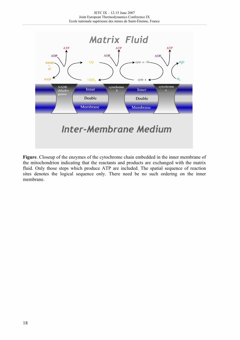
[email protected], [email protected] In mitochondria the large free energy of reaction between hydrogen and molecular oxygen is harvested in a number of steps by the cytochrome chain. We demonstrate the use of thermodynamic geometry and optimization at equipartition of thermodynamic distance through this biochemical example in computing the theoretically optimal sequence of energy degradation steps and comparing this with the actual energy steps in the cytochrome chain. This process is of keen interest because mitochondria are the fuel cells of the body. The context is nonetheless foreign to contemporary fuel cell design. Thus insights gained here are valuable for design questions generally and the energetic optimization of industrial fuel cells specifically. For process chains like the one considered here, the optimal operation, i.e. the operation with least dissipation, is achieved when the thermodynamic length of each step is the same. This thermodynamic length calculation uses a metric consisting of all the second derivatives of the entropy with respect to the other extensive coordinates, M=-(∂2S/∂Xi∂Xj). For this purpose we first calculate the full equation of state for a mixture of ideal gases,
∏⎥⎥⎥
⎦
⎤
⎢⎢⎢
⎣
⎡
⎟⎟⎠
⎞⎜⎜⎝
⎛=
j
Nn
j
Ck
jNCS
i
j
vvmV
nNeb)U(S,V,n 1
References
[1] W. A. Cramer, D. B. Knofff: Energy Transductions in Biological Membranes (Springer-Verlag, New York, 1990). [2] C. Eckart: The thermodynamics of irreversible processes I. The simple fluid. Phys. Rev. 58, 267-269 (1940). [3] C. Essex: Global thermodynamics, the Clausius inequality, and entropy of radiation. Geophys. Astrophys. Fluid Dynamics 38, 1-13 (1987). [4] J. Nulton, P. Salamon, B. Andresen, Q. Anmin: Quasistatic processes as step equilibrations. J. Chem. Phys.; 83, 334-338 (1985). [5] B. Andresen, P. Salamon: Optimal distillation using thermodynamic geometry; In: S. Sieniutycz, A. De Vos, editors: Thermodynamics of energy conversion and transport. (Springer-Verlag, New York, 2000), p. 319.
JETC IX – 12-15 June 2007 Joint European Thermodynamics Conference IX
Ecole nationale supérieure des mines de Saint-Étienne, France
18
Figure. Closeup of the enzymes of the cytochrome chain embedded in the inner membrane of the mitochondrion indicating that the reactants and products are exchanged with the matrix fluid. Only those steps which produce ATP are included. The spatial sequence of reaction sites denotes the logical sequence only. There need be no such ordering on the inner membrane.
JETC IX – 12-15 June 2007 Joint European Thermodynamics Conference IX
Ecole nationale supérieure des mines de Saint-Étienne, France
19
Liquid-liquid equilibrium in the binary system 1-butyl-3-methylimidazolium hexafluorophosphate + water.
Quantitative analysis of the experimental data
Magdalena Bendová, a Zdeněk Wagner, a Michal Moučka b
a Institute of Chemical Process Fundamentals, Academy of Sciences of the Czech Republic, Rozvojová 135, 165 02 Prague 6, Czech Republic
b Department of Applied Cybernetics, Technical University of Liberec, Hálkova 6, 461 17 Liberec. Czech Republic
[email protected] - [email protected] Abstract In the present contribution, liquid-liquid equilibrium in the binary system 1-butyl-3-methylimidazolium hexafluorophosphate (abbr. [bmim][PF6]) is investigated. Tie-lines were obtained by the volumetric method [1] and points of the binodal curve were measured by the cloud-point method. The former experiment consists of calculating the equilibrium compositions from the volumes of the equilibrium phases using simple mass balance formulas, whereas in the latter solution temperatures are determined synthetically in mixtures of known compositions. Both experimental apparatuses were built in our laboratory, the cloud-point method apparatus was developed in collaboration with the Technical University of Liberec. The experimental data were subsequently described by the modified Flory-Huggins equation proposed by de Sousa and Rebelo [2] and by the molecular-thermodynamic lattice model proposed by Qin and Prausnitz [3]. The choice of these models primarily designed for mixtures of polymers is based on findings that ionic liquids showed to some extent polymer-like behaviour [4, 5] and also on the previous successful use of the modified Flory-Huggins equation in descriptions of thermodynamic properties of mixtures of ionic liquids[1, 6, 7]. Gnostic regression approach [1] was used to obtain parameters of the thermodynamic models. This modelling approach also enabled us to compare the data acquired in this work with literature values [6, 8-14].
Introduction
There is an ever increasing interest in room-temperature ionic liquids (RTILs) as prospective more efficient and greener substitutes of volatile organic compounds. Knowledge of the liquid-liquid equilibria in binary and multicomponent systems is of essential importance in the design of fluid separation processes, and particularly extraction. Similarly important is the critical assessment of the obtained data and their comparison with existent literature ones; data concerning systems with ionic liquids often show large discrepancies, there is therefore a strong need for their reliable quantitative analysis. For this purpose, robust evaluation tools able to detect possible outliers and/or thermodynamically inconsistent data are necessary. In this work, liquid-liquid equilibrium in the binary system 1-butyl-3-methylimidazolium hexafluorophosphate + water was measured by means of the volumetric and cloud-point methods. The obtained data were correlated by the modified Flory-Huggins equation [2] and the molecular-thermodynamic lattice model proposed by Qin and Prausnitz [3]. Both models were primarily derived to describe mixtures of polymers, but their use for mixtures of ionic liquids seems justified by some findings showing that RTILs tend to present polymer-like
JETC IX – 12-15 June 2007 Joint European Thermodynamics Conference IX
Ecole nationale supérieure des mines de Saint-Étienne, France
20
behaviour [4, 5]. The experimental data acquired in the present work were also quantitatively compared with literature data. Both in the correlations and in the quantitative comparison of the individual datasets a gnostic regression method that enabled us to compare the data reliably was used.
Experimental In this work, 1-butyl-3-methylimidazolium hexafluorophosphate (abbr. [bmim][PF6]) was provided by Solvent Innovation (www.solvent-innovation.com) and was dried for at least 48 hrs under vacuum before the measurements. The water content determined using the Karl-Fischer titration in the dried ionic liquid was then found to be 50 ppm. Distilled water with conductivity 2.1 μS prepared in our laboratory was used in the experiments. To measure tie lines, a simple volumetric experiment was used. A volumetric apparatus was built in our laboratory and is described in previous work [1]. The experiment consists in measuring volumes of the equilibrium phases and in subsequent calculation of their compositions from mass balance. The experimental uncertainty estimated by means of the error-propagation law was found to be ± 0.02 and ± 0.0001 in mole fraction for the ionic-liquid phase and the aqueous phase respectively. To check the volumetric data, points of the solubility curve were measured by the cloud-point method. It consists in finding the solution temperature of a known mixture, i.e. the temperature at which a phase change occurs in the mixture. An apparatus built in our laboratory [1] was modified so that cloud-points could be determined with better accuracy and repeatability. Known amounts of both measured substances were weighed into a thermostated equilibrium cell and brought to a temperature at which the mixture became homogeneous. Then by means of a programmable thermostat, the temperature in the cell was reduced in a defined manner to find the narrowest possible temperature interval in which the phase change occurred. The cloud-point temperature was considered to be the temperature at which first droplets of the second phase appeared. The same procedure was repeated on rising the temperature, the clear-point temperature being the temperature at which the mixture became entirely homogeneous. Hysteresis in the read-outs of approx. 0.5 K was observed. The resulting solubility temperature was then determined as the average of the two readings. The phase changes were determined optically by measuring the intensity of light scattered by the mixture. A laser diode was the source of light, and a photodiode connected to a PC measuring card was used to detect the light signal. The temperature was measured directly in the thermostating jacket using a Pt100 platinum resistance thermometer; it was connected over a conversion unit to the measuring card. The measurements were monitored using a Labview 8.01 data acquisition application. The temperature conversion unit has been modified for this purpose at the Technical University of Liberec where the data aquisition application was also programmed. The experimental uncertainty of the cloud-point method was estimated to be ± 0.0002 in mole fraction, temperature was measured with an uncertainty of ± 0.02 K.
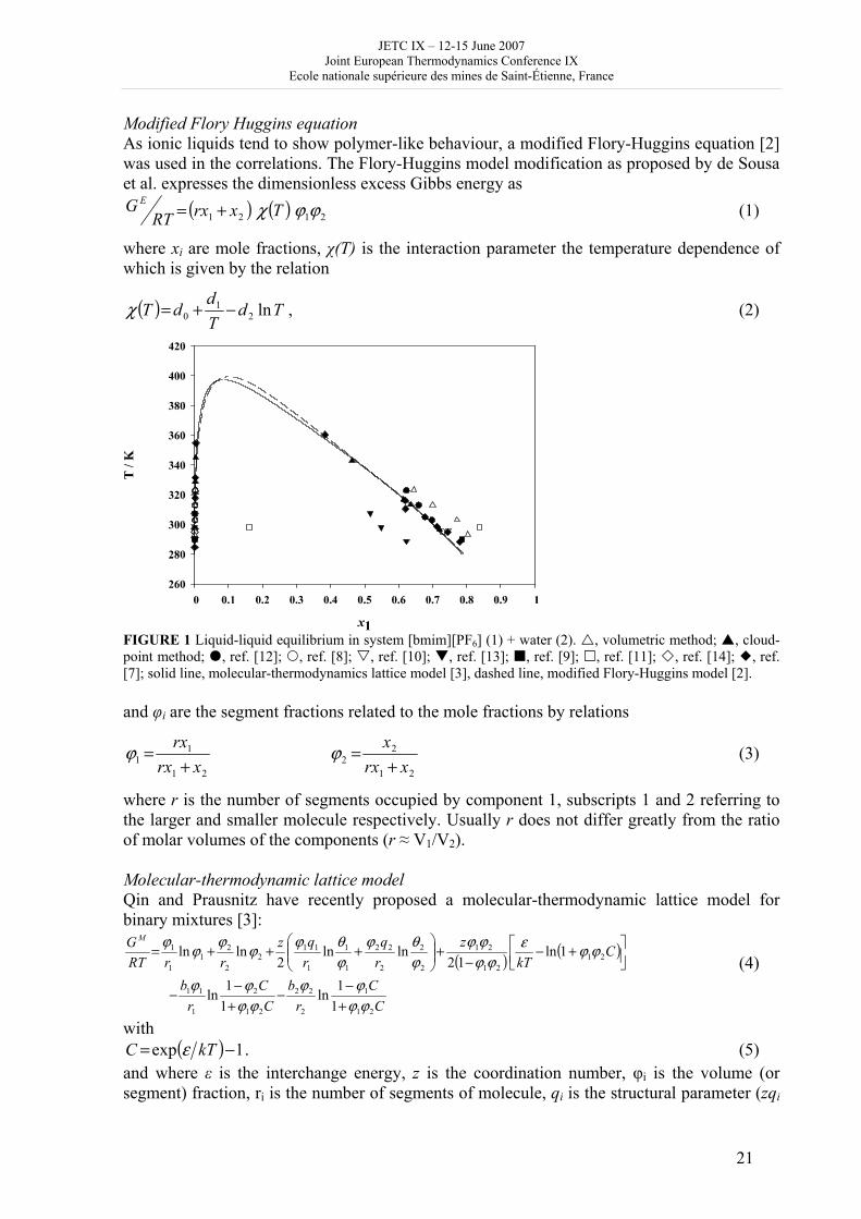
Results and Discussion In Figure 1, experimental results obtained in this work are compared with literature data and with thermodynamic description of all the datasets by the modified Flory-H uggins equation and the molecular-thermodynamic lattice model proposed by Qin and Prausnitz. Considering the experimental uncertainties found for both methods, the data obtained by the two experiments appear to be in good agreement. Agreement of our data with the literature values was evaluated quantitatively in the correlations described below.
JETC IX – 12-15 June 2007 Joint European Thermodynamics Conference IX
Ecole nationale supérieure des mines de Saint-Étienne, France
21
Modified Flory Huggins equation As ionic liquids tend to show polymer-like behaviour, a modified Flory-Huggins equation [2] was used in the correlations. The Flory-Huggins model modification as proposed by de Sousa et al. expresses the dimensionless excess Gibbs energy as
( ) ( ) 2121 ϕϕχ TxrxRTG E
+= (1)
where xi are mole fractions, χ(T) is the interaction parameter the temperature dependence of which is given by the relation
( ) TdTd
dT ln21
0 −+=χ , (2)
FIGURE 1 Liquid-liquid equilibrium in system [bmim][PF6] (1) + water (2). , volumetric method; , cloud-point method; , ref. [12]; , ref. [8]; , ref. [10]; , ref. [13]; , ref. [9]; , ref. [11]; , ref. [14]; , ref. [7]; solid line, molecular-thermodynamics lattice model [3], dashed line, modified Flory-Huggins model [2]. and φi are the segment fractions related to the mole fractions by relations
21
11 xrx
rx+
=ϕ 21
22 xrx
x+
=ϕ (3)
where r is the number of segments occupied by component 1, subscripts 1 and 2 referring to the larger and smaller molecule respectively. Usually r does not differ greatly from the ratio of molar volumes of the components (r ≈ V1/V2). Molecular-thermodynamic lattice model Qin and Prausnitz have recently proposed a molecular-thermodynamic lattice model for binary mixtures [3]:
( ) ( )
CC
rb
CC
rb
CkT
zrq
rqz
rrRTG M
21
1
2
22
21
2
1
11
2121
21
2
2
2
22
1
1
1
112
2
21
1
1
11
ln11
ln
1ln12
lnln2
lnln
ϕϕϕϕ
ϕϕϕϕ
ϕϕεϕϕ
ϕϕϕθϕ
ϕθϕϕϕϕϕ
+−
−+−
−
⎥⎦⎤
⎢⎣⎡ +−
−+⎟⎟⎠
⎞⎜⎜⎝
⎛+++=
(4)
with ( ) 1exp −= kTC ε . (5)
and where ε is the interchange energy, z is the coordination number, φi is the volume (or segment) fraction, ri is the number of segments of molecule, qi is the structural parameter (zqi
JETC IX – 12-15 June 2007 Joint European Thermodynamics Conference IX
Ecole nationale supérieure des mines de Saint-Étienne, France
22
is the surface of molecule) , bi is the number of chemical bonds of the molecule, θi is the surface fraction defined as
2211 NqNqNq ii
i +=θ (6)
Ni being the number of lattice sites occupied by molecule. The interchange energy temperature dependence is linear:
BTAk
+=⎟⎠⎞
⎜⎝⎛ εln (7)
Parameters of both models were optimized using a regression along a gnostic influence function [1]. Outliers were detected for all the datasets available. Mathematical processing of the data was improved in this work; whereas in our previous paper, tie lines were treated as two cloud-points, i.e. independently of each other, in this work they were processed as interrelated values. Table 1 gives the optimized parameters for the modified Flory-Huggins equation. The standard deviations were found to be 0.060 and 0.0014 for the ionic liquid and the aqueous phase respectively. TABLE 1 Parameters of the modified Flory-Huggins equation
r d0 d1 d2 4.2599 -30.5135 2599.58 -4.1915
Table 2 gives parameters for the molecular-thermodynamic lattice model with standard deviations 0.060 and 0.00088 for the ionic liquid and the aqueous phase respectively. TABLE 2 Constants of the Molecular-thermodynamic Lattice Model in System [bmim][PF6] (1) + water (2)
A B θ1 θ2
All the datasets, including the literature values were correlated simultaneously, which enabled us to compare the data quantitatively. As is evident from the acquired standard deviations, both our data and the literature ones are in good mutual agreement, the only outliers being the values by Swatloski et al. [11].
Conclusions Liquid-liquid equilibrium and points of binodal curve were obtained in this work and compared with available literature data. To describe and correlate the available datasets, the modified Flory-Huggins and a molecular-thermodynamic lattice model by Qin and Prausnitz were used, with parameter optimization being carried out by a gnostic regression method. The data appear to be in good mutual agreement, both models yielding a good description of the experimental values. Acknowledgment This work was supported by the Czech Science Foundation under grant No. 104/03/1555.
JETC IX – 12-15 June 2007 Joint European Thermodynamics Conference IX
Ecole nationale supérieure des mines de Saint-Étienne, France
23
References
1. Bendová, M.; Wagner, Z. J. Chem. Eng. Data 2006, 51, 2126 – 2131. 2. De Sousa, H. C.; Rebelo, L. P. N. A J. Polym. Sci. B: Polym. Phys. 2000, 38, 632 –
651. 3. Qin, Y.; Prausnitz, J. M. Z. Phys. Chem. 2005, 219, 1223 – 1241. 4. Kazarian, S. G.; Briscoe, B. J.; Welton T. Chem. Commun. 2000, 2047 – 2048. 5. Dupont, J.; de Souza, F.; Suarez, P. A. Z. Chem. Rev. 2002, 102, 3667 – 3692. 6. Najdanovic-Visak, V; Esperança, J. M. S. S.; Rebelo, L. P. N.; Da Ponte, M. N.;
Guedes, H. J. R.; Seddon, K. R.; De Sousa, H. C.; Szydlowski, J. J. Phys. Chem. B 2003, 107, 12797 – 12807.
7. Rebelo, L. P. N.; Najdanovic-Visak, V.; Visak, Z. P.; Nunes da Ponte, M.; Szydlowski, J.; Cerdeiriña, C. A.; Troncoso, J.; Romaní, L.; Esperança, J. M. S. S.; Guedes, H. J. R.; De Sousa, H. C. Green. Chem. 2004, 6, 369 – 381.
8. Anthony, J.L.; Maginn, E.J.; Brennecke, J.F. J. Phys. Chem. B 2001, 105, 10942 – 10949.
9. Chun, S.; Dzyuba, S.V.; Bartsch, R.A. Anal. Chem. 2001, 73, 3737 – 3741. 10. Fadeev, A.G.; Meagher, M.M. Chem. Commun. 2001, 3, 295 – 296. 11. Swatloski, R.P.; Visser, A.E.; Reichhert, W.M.; Broker, G.A.; Farina, L.M.;
Holbrey, J.D.; Rogers, R.D. Green Chem. 2002, 4, 81 – 87. 12. Wong, D.S.H.; Chen, J.P.; Chang, J.M.; Chou, C.H. Fluid Phase Equilibria 2002,
194 – 197, 1089 – 1095. 13. Wu, C.-T. Thermophysical Properties of Room-Temperature Ionic Liquids and
Their Mixtures, MSc Thesis. 14. McFarlane, J.; Ridenour, W.B.; Luo, H.; Hunt, R.D.; de Paoli, D.W. Sep. Sci. Tech.
2005, 40, 1245 – 1265.
JETC IX – 12-15 June 2007 Joint European Thermodynamics Conference IX
Ecole nationale supérieure des mines de Saint-Étienne, France
24
Axiomatic definition of entropy for nonequilibrium states
Gian Paolo Beretta
Università di Brescia, Italy
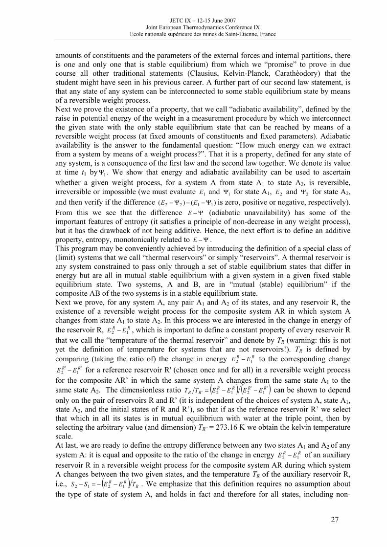
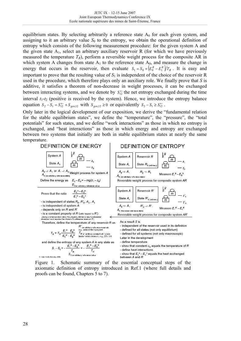
[email protected] Abstract In introductory courses and textbooks on elementary thermodynamics, entropy is often presented as a property defined only for equilibrium states, and its axiomatic definition is almost invariably given in terms of a heat to temperature ratio. We have devised a simple, non-mathematical axiomatic definition valid for all states, including non-equilibrium states (for which temperature is not defined). We have used it successfully in undergraduate and graduate courses for the past thirty years. It is based on the essential elements of the definition developed with full proofs in the treatise1 E.P. Gyftopoulos and G.P. Beretta, Thermodynamics. Foundations and Applications, Dover edition, 2005 (first edition, Macmillan, 1991). In our presentation at this conference, we illustrate the above logic of exposition, mainly by means of the viewgraph reported in Figure 1, which summarizes the essential elements of our general axiomatic definition of entropy valid for non-equilibrium states no matter how “far” from thermodynamic equilibrium. The reader is referred to our book1 for full details.
Introduction In this short paper, we comment on the motivation by which the “MIT school of thermodynamics” (Keenan, Hatsopoulos, Gyftopoulos, Beretta, Zanchini) has developed a logical sequence of exposition of the axiomatic foundations of thermodynamics in which entropy is defined before heat, and not viceversa as in most other presentations. We emphasize the important essential hypotheses and logical steps of our unconventional order of exposition, which was developed as a means to remove the well-known logical loop which is unavoidable in the traditional definition of entropy based on a heat to temperature ratio, due to the fact that heat and temperature are almost invariably ill defined by means of some heuristic arguments by which heat is introduced in terms of mechanical illustrations aimed at “demonstrating” the difference between heat and work. For example, in his lectures on physics that have influenced many generations of physicists, Feynman2 describes heat as one of several different forms of energy, related to the “jiggling” motion of particles stuck together and tagging along with each other (pp.1-3 and 4-2), a “form of energy” which really is just kinetic energy—internal motion (p.4-6), and is measured by random motions of the atoms (p.10-8). Tisza3 argues that such slogans as “heat is motion”, in spite of their fuzzy meaning, convey intuitive images of pedagogical and heuristic value. There are at least two problems with these illustrations. First, work and heat are not “stored” in a system. Each is a mode of transfer of energy between interacting systems. Second, and perhaps most important, concepts of mechanics are used to justify and make plausible a notion—that of heat—which is beyond the realm of mechanics. In spite of these logical drawbacks, the trick works because at first the student finds the idea of heat harmless, and even intuitive. But the situation changes drastically and irrecoverably as soon as the notion of heat is used to define a host of new non-mechanical ideas, less intuitive and less harmless. At once, heat is raised to the same dignity as work, it is contrasted to work and used as an
JETC IX – 12-15 June 2007 Joint European Thermodynamics Conference IX
Ecole nationale supérieure des mines de Saint-Étienne, France
25
essential ingredient in the first law. The student begins to worry because the notion of heat is less definite and not as operational as that of work. The first problem is addressed in some expositions. Landau and Lifshitz4 define heat as the part of an energy change on a body that is not due to work done on it. Guggenheim5 defines heat as an exchange of energy that differs from work and is determined by a temperature difference. Keenan6 defines heat as the energy transferred from one system to a second system at lower temperature, by virtue of a temperature difference, when the two are brought into communication. Similar definitions are adopted in notable textbooks, such as Van Wylen and Sonntag,7 Wark,8 Huang,9 Modell and Reid,10 Moran and Shapiro,11 and Bejan.12 None of these definitions, however, addresses the basic problem. The existence of exchanges of energy that differ from work is not granted by mechanics, not even (in our view) after the recent vaste physics literature on quantum theories of open systems13 which has addressed, directly or indirectly, this issue. Indeed, such existence is one of the striking results of thermodynamics, that is, of the existence of entropy as a property of matter. Hatsopoulos and Keenan14 have pointed out explicitly that without the second law heat and work would be indistinguishable and, therefore, a satisfactory definition of heat is unlikely without a prior statement of the second law. In our experience, whenever heat is introduced before the first law, and then used in the statement of the second law and in the definition of entropy, the student cannot avoid but sense ambiguity and lack of logical consistency. This results in the wrong but unfortunately widespread conviction that thermodynamics is a confusing, ambiguous, hand-waving, phenomenological subject. Teaching thermodynamics at MIT to generations of graduate students from all regions of the globe has evidenced the need for more clarity, unambiguity and logical consistency in the exposition of general thermodynamic principles than provided by traditional approaches. Continuing the effort pioneered at MIT by Keenan,6 Hatsopoulos and Keenan,14 and Hatsopoulos and Gyftopoulos,15,16 Gyftopoulos and the present author1 have composed an exposition which strives to develop the basic concepts unambiguously and with rigorous logical consistency, building upon the student’s sophomore background in introductory physics and mechanics. The basic concepts and principles are introduced in a novel sequence that eliminates the problem of incomplete or heuristic definitions, and that is valid for both macroscopic and microscopic well-defined systems, and for both equilibrium and nonequilibrium states. The laws of thermodynamics are presented as general consequences of the fundamental dynamical laws of physics that hold for all well-defined systems. In engineering presentations, like that in Ref.1, they are presented as laws, rather than theorems of the fundamental dynamical laws, so as to develop a level of description that avoids the full mathematical technicalities required to express such dynamical laws. However, we do not restrict our attention only to the equilibrium domain. Our definition of entropy is more general than that of most textbook where, as Callen17 stresses, the existence of the entropy is postulated only for equilibrium states and the postulate makes no reference whatsoever to nonequilibrium states. Heat plays no role in our statement of the first law, in the definition of energy, in our statement of the second law, in the definition of entropy, and in the concepts of energy and entropy exchanges between interacting systems. It is defined using these concepts and laws, after they have been independently and unambiguously introduced. Heat is the energy exchanged between systems that interact under very restrictive conditions that define what we call a heat interaction. Schematic outline of our exposition of the foundations of thermodynamics up to our axiomatic definition of entropy valid for equilibrium and nonequilibrium states
JETC IX – 12-15 June 2007 Joint European Thermodynamics Conference IX
Ecole nationale supérieure des mines de Saint-Étienne, France
26
Here we outline schematically the logical sequence of exposition that we adopt in our book1, to which the reader is referred to for full details and proofs. In an undergraduate course focused on engineering applications, in class we skip most proofs (interested students can find them in the book) and in about eight to ten 45-min lectures we develop the foundations of the subject in following sequence. We define the scope of thermodynamics as that of describing the properties of physical systems and how they evolve in time. We define what we mean by a well-defined “system” (constituents; amounts of constituents; internal forces, internal partitions, external forces and parameters; examples of nonseparable objects that cannot be a well-defined system). We define what we mean by “property” (repeatable measurement procedure yielding a numerical result that depends only on one instant in time) and “state” (list of values at one instant in time of all the amounts of constituents, all the parameters of the external forces, and all the conceivable properties of the system). We explain that a full description of how the state of the system evolves in time requires the consideration and solution of its general equation of motion. Instead of taking this approach, which is postponed to more advanced and theoretical treatments, we focus on the two most general theorems of the equation of motion, that are universal features of the dynamics of all well-defined systems. Such theorems are captured by two general non-mathematical statements valid for all systems. We call these statements “principles” or “laws” because in our exposition they are not proved from the analysis of the equation of motion, but are adopted and assumed as the dynamical features that cannot be violated by the evolution of any well-defined system. To move towards the statements of these two laws, we introduce the concepts of “process” (initial and final states of a system; description of the effects left in its environment, the rest of the Universe), “spontaneous change of state”, “isolated system”, and “weight process” (the only external effect is the change in height of a weight). We state the “first law” (every pair of states of any given system can be interconnected by means of a weight process) and prove that it entails the existence of a property, that we call “energy”, defined by a measurement procedure by which we interconnect the given state and an arbitrary reference state (selected once and for all for the system) by means of a weight process and measure the change in potential energy of the weight (potential energy of a simple weight is a known concept from previous courses in mechanics). We emphasize that, by virtue of the first law, the concept of energy is thus extended from the domain of mechanics to the broader domain of thermodynamics. We then show that energy is an “additive” property, it is “conserved” (remains constant in spontaneous changes of state, and for isolated systems), and it can be exchanged between interacting systems; we denote by
←12E the net energy exchanged during the time interval t1-t2 (positive is received by the
system). Hence, we introduce the energy balance equation ←=− 1212 EEE . To introduce the second law, we define a “reversible process” (if a process exists that takes the system back to its initial state while all external effects are undone) and in particular a “reversible weight process” (if a weight process exists that takes the system back to its initial state while all external effects are undone). We then classify states in terms of their time dependence (steady, unsteady, equilibrium and non-equilibrium). We further classify equilibrium states in terms of their stability (unstable, metastable, and stable). A “stable equilibrium state” is one that cannot be altered without leaving net effects in the environment of the system (as shown in Ref.18, this is a non-mathematical expression of the definition of stability according to Lyapunov). The second law is introduced as the answer to the question: “How many stable equilibrium states does a system admit?”, a question that clearly addresses a fundamental feature of the dynamics. The answer is the Hatsopoulos-Keenan statement of the “second law” (among all the states of a system that have given values of the energy, the
JETC IX – 12-15 June 2007 Joint European Thermodynamics Conference IX
Ecole nationale supérieure des mines de Saint-Étienne, France
27
amounts of constituents and the parameters of the external forces and internal partitions, there is one and only one that is stable equilibrium) from which we “promise” to prove in due course all other traditional statements (Clausius, Kelvin-Planck, Carathèodory) that the student might have seen in his previous career. A further part of our second law statement, is that any state of any system can be interconnected to some stable equilibrium state by means of a reversible weight process. Next we prove the existence of a property, that we call “adiabatic availability”, defined by the raise in potential energy of the weight in a measurement procedure by which we interconnect the given state with the only stable equilibrium state that can be reached by means of a reversible weight process (at fixed amounts of constituents and fixed parameters). Adiabatic availability is the answer to the fundamental question: “How much energy can we extract from a system by means of a weight process?”. That it is a property, defined for any state of any system, is a consequence of the first law and the second law together. We denote its value at time t1 by 1Ψ . We show that energy and adiabatic availability can be used to ascertain whether a given weight process, for a system A from state A1 to state A2, is reversible, irreversible or impossible (we must evaluate 1E and 1Ψ for state A1, 2E and 2Ψ for state A2, and then verify if the difference )()( 1122 Ψ−−Ψ− EE is zero, positive or negative, respectively). From this we see that the difference Ψ−E (adiabatic unavailability) has some of the important features of entropy (it satisfies a principle of non-decrease in any weight process), but it has the drawback of not being additive. Hence, the next effort is to define an additive property, entropy, monotonically related to Ψ−E . This program may be conveniently achieved by introducing the definition of a special class of (limit) systems that we call “thermal reservoirs” or simply “reservoirs”. A thermal reservoir is any system constrained to pass only through a set of stable equilibrium states that differ in energy but are all in mutual stable equilibrium with a given system in a given fixed stable equilibrium state. Two systems, A and B, are in “mutual (stable) equilibrium” if the composite AB of the two systems is in a stable equilibrium state. Next we prove, for any system A, any pair A1 and A2 of its states, and any reservoir R, the existence of a reversible weight process for the composite system AR in which system A changes from state A1 to state A2. In this process we are interested in the change in energy of the reservoir R, RR EE 12 − , which is important to define a constant property of every reservoir R that we call the “temperature of the thermal reservoir” and denote by TR (warning: this is not yet the definition of temperature for systems that are not reservoirs!). TR is defined by comparing (taking the ratio of) the change in energy RR EE 12 − to the corresponding change
'1
'2
RR EE − for a reference reservoir R' (chosen once and for all) in a reversible weight process for the composite AR’ in which the same system A changes from the same state A1 to the same state A2. The dimensionless ratio ( ) ( )'
1'
212'RRRR
RR EEEETT −−= can be shown to depend only on the pair of reservoirs R and R’ (it is independent of the choices of system A, state A1, state A2, and the initial states of R and R’), so that if as the reference reservoir R’ we select that which in all its states is in mutual equilibrium with water at the triple point, then by selecting the arbitrary value (and dimension) TR’ = 273.16 K we obtain the kelvin temperature scale. At last, we are ready to define the entropy difference between any two states A1 and A2 of any system A: it is equal and opposite to the ratio of the change in energy RR EE 12 − of an auxiliary reservoir R in a reversible weight process for the composite system AR during which system A changes between the two given states, and the temperature TR of the auxiliary reservoir R, i.e., ( ) R
RR TEESS 1212 −−=− . We emphasize that this definition requires no assumption about the type of state of system A, and holds in fact and therefore for all states, including non-
JETC IX – 12-15 June 2007 Joint European Thermodynamics Conference IX
Ecole nationale supérieure des mines de Saint-Étienne, France
28
equilibrium states. By selecting arbitrarily a reference state A0 for each given system, and assigning to it an arbitrary value S0 to the entropy, we obtain the operational definition of entropy which consists of the following measurement procedure: for the given system A and the given state A1, select an arbitrary auxiliary reservoir R (for which we have previously measured the temperature TR), perform a reversible weight process for the composite AR in which system A changes from state A1 to the reference state A0, and measure the change in energy that occurs in the reservoir, then evaluate ( ) R
RR TEESS 1001 −+= . It is easy and important to prove that the resulting value of S1 is independent of the choice of the reservoir R used in the procedure, which therefore plays only an auxiliary role. We finally prove that S is additive, it satisfies a theorem of non-decrease in weight processes, it can be exchanged between interacting systems, and we denote by ←
12S the net entropy exchanged during the time interval t1-t2 (positive is received by the system). Hence, we introduce the entropy balance equation 12,1212 genSSSS +=− ← with 012, ≥genS or equivalently ←≥− 1212 SSS . Only later in the logical development of our exposition, we derive the “fundamental relation for the stable equilibrium states”, we define the “temperature”, the “pressure”, the “total potentials” for such states, and we define “work interactions” as those in which no entropy is exchanged, and “heat interactions” as those in which energy and entropy are exchanged between two systems that initially are both in stable equilibrium states at nearly the same temperature.
Figure 1. Schematic summary of the essential conceptual steps of the axiomatic definition of entropy introduced in Ref.1 (where full details and proofs can be found, Chapters 5 to 7).
JETC IX – 12-15 June 2007 Joint European Thermodynamics Conference IX
Ecole nationale supérieure des mines de Saint-Étienne, France
29
References
1. E.P. Gyftopoulos and G.P. Beretta, Thermodynamics. Foundations and Applications, Dover, Mineola, 2005 (first edition, Macmillan, 1991). 2. R.P. Feynman, Lectures on Physics, Vol.1, Addison-Welsey, 1963. 3. L. Tisza, Generalized Thermodynamics, MIT Press, 1966, p.16. 4. L.D. Landau and E.M. Lifshitz, Statistical Physics, Part I, 3rd Ed., Revised by E.M. Lifshitz and L.P. Pitaevskii, Translated by J.B. Sykes and M.J. Kearsley, Pergamon Press, 1980, p.45. 5. E.A. Guggenheim, Thermodynamics, North-Holland, 7th Ed., 1967, p.10. 6. J.H. Keenan, Thermodynamics, Wiley, 1941, p.6. 7. G.J. Van Wylen and R.E. Sonntag, Fundamentals of Classical Thermodynamics, Wiley, 2nd Ed., 1978, p.76. 8. K. Wark, Thermodynamics, 4th Ed., McGraw-Hill, 1983, p.43. 9. F.F. Huang, Engineering Thermodynamics, Macmillan, 1976, p.47. 10. M. Modell and R.C. Reid, Thermodynamics and Its Applications, Prentice-Hall, 1983, p.29. 11. M.J. Moran and H.N. Shapiro, Fundamentals of Engineering Thermodynamics, Wiley, 1988, p.46. 12. A. Bejan, Advanced Engineering Thermodynamics, 2nd Ed., Wiley, 1997. 13. H.P. Breuer and F. Petruccione, The Theory of Open Quantum Systems, Oxford University Press, 2002. 14. G.N. Hatsopoulos and J.H. Keenan, Principes of General Thermodynamics, Wiley, 1965, p.xxiii. 15. G.N. Hatsopoulos and E.P Gyftopoulos, Foundations of Physics, Vol. 6, 15, 127, 439, 561 (1976). 16. G.N. Hatsopoulos and E.P Gyftopoulos, Thermionic Energy Conversion, Vol. II, MIT Press, 1979. 17. H.B. Callen, Thermodynamics, and an Introduction to Thermostatics, 2nd Ed., Wiley, 1985. 18. G.P. Beretta, Journal of Mathematical Physics, Vol. 27, 305 (1986).
JETC IX – 12-15 June 2007 Joint European Thermodynamics Conference IX
Ecole nationale supérieure des mines de Saint-Étienne, France
30
Nonlinear Generalization of Schrödinger's Equation Uniting Quantum Mechanics and Thermodynamics
Gian Paolo Beretta
Università di Brescia, Italy
[email protected] - www.quantumthermodynamics.org Abstract We discuss and motivate the form of a nonlinear equation of motion that accomplishes a self-consistent unification of quantum mechanics (QM) and thermodynamics conceptually different from the (von Neumann) foundations of quantum statistical mechanics (QSM) and (Jaynes) quantum information theory (QIT), but which reduces to the same mathematics for the thermodynamic equilibrium (TE) states, and contains standard QM in that it reduces to the time-dependent Schrödinger equation for zero entropy states. By restricting the discussion to a strictly isolated system (non-interacting, disentangled and uncorrelated) we show how the theory departs from the conventional QSM/QIT rationalization of the second law of thermodynamics, which instead emerges in QT as a theorem of existence and uniqueness of a stable equilibrium state for each set of mean values of the energy and the number of constituent particles. To achieve this, the theory assumes -kBTr(ρlnρ) for the physical entropy and is designed to implement two fundamental ansatzs: (1) that in addition to the standard QM states described by idempotent density operators (zero entropy), a strictly isolated and uncorrelated system admits also states that must be described by non-idempotent density operators (nonzero entropy); (2) that for such additional states the law of causal evolution is determined by the simultaneous action of a Schrödinger-von Neumann-type Hamiltonian generator and a nonlinear dissipative generator which conserves the mean values of the energy and the number of constituent particles, and in forward time drives the density operator in the 'direction' of steepest entropy ascent (maximal entropy generation). The resulting dynamics is well-defined for all non-equilibrium states, no matter how far from TE. Existence and uniqueness of solutions of the Cauchy initial value problem for all density operators, implies that the equation of motion can be solved not only in forward time, to describe relaxation towards TE, but also in backward time, to reconstruct the 'ancestral' or primordial lowest entropy state or limit cycle from which the system originates. Zero entropy states as well as a well-defined family of non-dissipative states evolve unitarily according to pure Hamiltonian dynamics and can be viewed as unstable limit cycles of the general nonlinear dynamics. For a review and the essential mathematical details of the theory the reader is referred to G.P. Beretta, “Positive nonlinear dynamical group uniting quantum mechanics and thermodynamics”, quant-ph/0612215, 2006. Thermodynamics after Prigogine The two fundamental ansatzs of QT have been formulated in a series of papers (see the bibliography cited below and that available at www.quantumthermodynamics.org) published since 1976 by various members of the MIT school of thermodynamics (Keenan, Hatsopoulos, Gyftopoulos, Park, Beretta, Çubukçu, von Spakovsky). The theory has been defined “an adventurous scheme which seeks to incorporate thermodynamics into the quantum laws of motion, and may end arguments about the arrow of time – but only if it works” by J. Maddox, Nature, Vol.316, 11 (1985), and it has been recently rediscovered and re-evaluated by S. Gheorghiu-Svirschevski, Phys. Rev. A, Vol. 63, 054102 (2001). It accomplishes from a
JETC IX – 12-15 June 2007 Joint European Thermodynamics Conference IX
Ecole nationale supérieure des mines de Saint-Étienne, France
31
different perspective the program that Prigogine and coauthors of the Brussels school have set out during the same period, to seek a formulation of the microscopic foundations of physical entropy and irreversibility. For this reason, even though our approach is very different from that of the Brussels school, I suggest that in a broad sense it does accomplish what Prigogine always felt it ought to be possible to do to formulate a theory in which entropy emerges as an intrinsic objective physical property and irreversibility as an objective dynamical aspect of microscopic physical reality. Quantum Thermodynamics and the MIT School of Thermodynamics According to QSM and QIT, the uncertainties that are measured by the physical entropy, are to be regarded as either extrinsic features of the heterogeneity of an ensemble or as witnesses of correlations with other systems. Instead, we have developed a self-consistent alternative theory, that we originally1,2 named Quantum Thermodynamics (QT) although in recent years the same name has been adopted losely in a wide variety of contexts without reference whatsoever to our theory. Our QT is based on the Hatsopoulos-Gyftopoulos fundamental ansatz3 that the uncertainties measured by the physical entropy are irreducible and hence, “physically real” and “objective” like standard QM uncertainties, that they belong to the state of the individual system, even if uncorrelated and even if a member of a “homogeneous ensemble” (in the von Neumann sense4). According to QT, second law limitations emerge as manifestations of such additional physical and irreducible uncertainties.3 The Hatsopoulos-Gyftopoulos ansatz (illustrated in Figure 1 for the simplest quantum system, a “qubit”, i.e., a two-level system) not only makes a unified theory of QM and Thermodynamics possible, but gives also a framework for a resolution of the century old “irreversibility paradox”, as well as of the conceptual paradox5 about the QSM/QIT interpretation of density operators, which has preoccupied scientists and philosophers since when Schroedinger surfaced it in Ref. 6. The Hatsopoulos-Gyftopoulos fundamental ansatz seems to respond to Schroedinger’s prescient conclusion:6 “…in a domain which the present theory (Quantum Mechanics) does not cover, there is room for new assumptions without necessarily contradicting the theory in that region where it is backed by experiment.” QT has been described7 as “an adventurous scheme”, and indeed it requires quite a few conceptual and interpretational jumps, but (1) it does not contradict any of the mathematics of either standard QM or TE QSM/QIT, which are both contained as extreme cases of the unified theory, and (2) for nonequilibrium states, no matter how “far” from TE, it offers the structured, nonlinear equation of motion proposed by this author2,8,9 which models, deterministically, irreversibility, relaxation and decoherence, and is based on the additional ansatz of steepest-entropy-ascent10-12 microscopic dynamics. Many authors, in a variety of contexts,13,14 have observed in recent years that irreversible natural phenomena at all levels of description seem to obey a principle of general and unifying validity. It has been named “maximum entropy production principle”, but we note in this paper that, at least at the quantum level, the weaker concept2,10,12 of “attraction towards the direction of steepest entropy ascent” is sufficient to capture precisely the essence of the (general Hatsopoulos-Keenan statement15,16 of the) second law. We emphasize that the steepest-entropy-ascent, nonlinear law of motion we formulated, and the dynamical group it generates17-19 (not just a semi-group), is a potentially powerful modeling tool that should find immediate application also outside of QT, namely, regardless of the dispute about the validity of the Hatsopoulos-Gyftopoulos ansatz on which QT hinges. Indeed, in view of its well-defined and well-behaved general mathematical features and solutions, our equation of motion may be used in phenomenological kinetic and dynamical theories where there is a need to guarantee full compatibility with the principle of entropy non-decrease and the second-law requirement of existence and uniqueness of stable
JETC IX – 12-15 June 2007 Joint European Thermodynamics Conference IX
Ecole nationale supérieure des mines de Saint-Étienne, France
32
equilibrium states (for each set of values of the mean energy, of boundary-condition parameters, and of the mean amount of constituents).
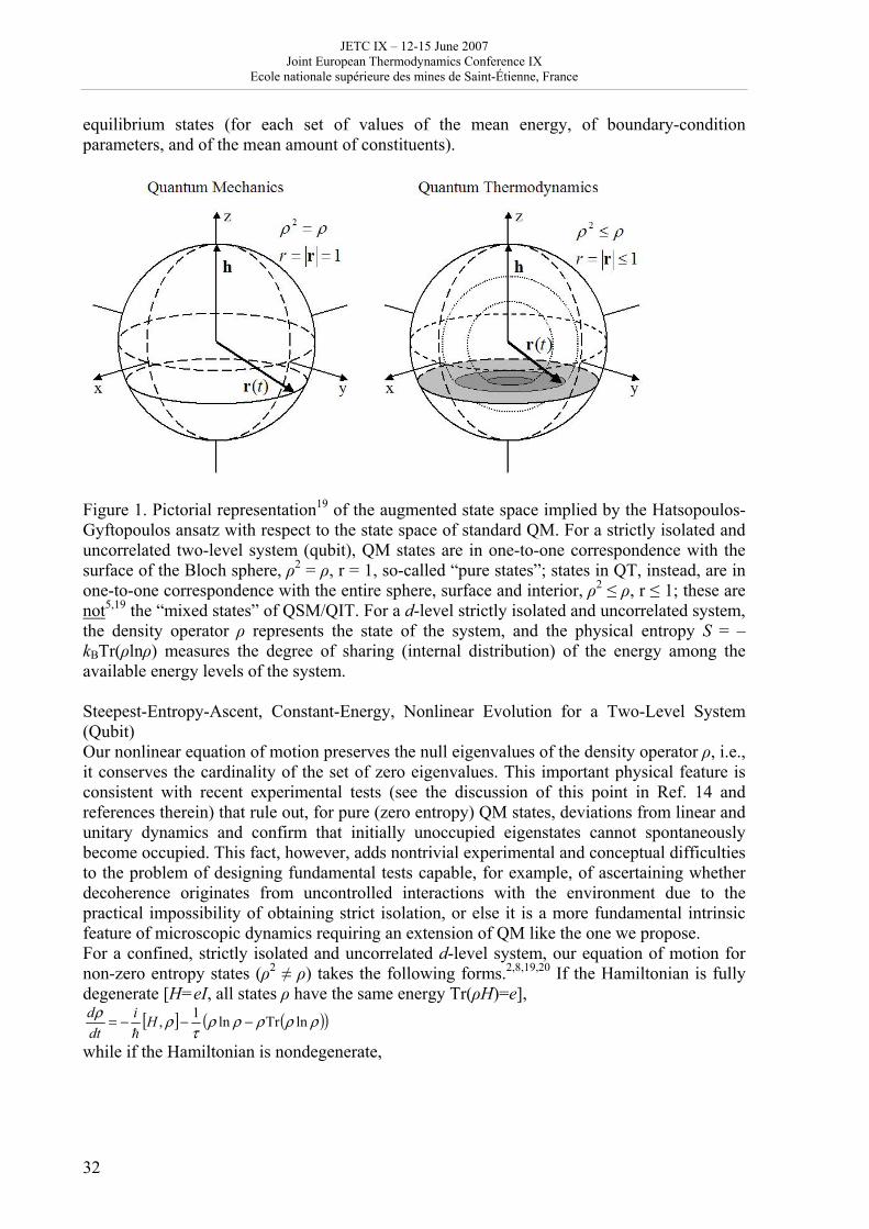
Figure 1. Pictorial representation19 of the augmented state space implied by the Hatsopoulos-Gyftopoulos ansatz with respect to the state space of standard QM. For a strictly isolated and uncorrelated two-level system (qubit), QM states are in one-to-one correspondence with the surface of the Bloch sphere, ρ2 = ρ, r = 1, so-called “pure states”; states in QT, instead, are in one-to-one correspondence with the entire sphere, surface and interior, ρ2 ≤ ρ, r ≤ 1; these are not5,19 the “mixed states” of QSM/QIT. For a d-level strictly isolated and uncorrelated system, the density operator ρ represents the state of the system, and the physical entropy S = – kBTr(ρlnρ) measures the degree of sharing (internal distribution) of the energy among the available energy levels of the system. Steepest-Entropy-Ascent, Constant-Energy, Nonlinear Evolution for a Two-Level System (Qubit) Our nonlinear equation of motion preserves the null eigenvalues of the density operator ρ, i.e., it conserves the cardinality of the set of zero eigenvalues. This important physical feature is consistent with recent experimental tests (see the discussion of this point in Ref. 14 and references therein) that rule out, for pure (zero entropy) QM states, deviations from linear and unitary dynamics and confirm that initially unoccupied eigenstates cannot spontaneously become occupied. This fact, however, adds nontrivial experimental and conceptual difficulties to the problem of designing fundamental tests capable, for example, of ascertaining whether decoherence originates from uncontrolled interactions with the environment due to the practical impossibility of obtaining strict isolation, or else it is a more fundamental intrinsic feature of microscopic dynamics requiring an extension of QM like the one we propose. For a confined, strictly isolated and uncorrelated d-level system, our equation of motion for non-zero entropy states (ρ2 ≠ ρ) takes the following forms.2,8,19,20 If the Hamiltonian is fully degenerate [H=eI, all states ρ have the same energy Tr(ρH)=e],
[ ] ( )( )ρρρρρτ
ρρ lnTrln1, −−−= Hidtd
h
while if the Hamiltonian is nondegenerate,
JETC IX – 12-15 June 2007 Joint European Thermodynamics Conference IX
Ecole nationale supérieure des mines de Saint-Étienne, France
33
[ ]
{ }( ) ( )
( ) ( ) ( )( ) ( )[ ]22
2
TrTr
TrTrlnTrTr1lnTr
,21ln
1,HH
HHHH
H
Hidtd
ρρ
ρρρρρρρ
ρρρρ
τρρ
−−−=
h
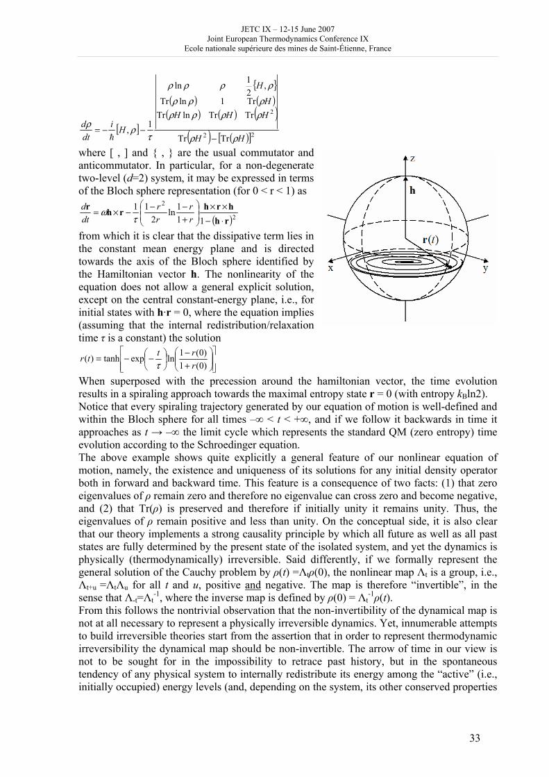
where [ , ] and { , } are the usual commutator and anticommutator. In particular, for a non-degenerate two-level (d=2) system, it may be expressed in terms of the Bloch sphere representation (for 0 < r < 1) as
( )2
2
111ln
211
rhhrhrhr
⋅−××
⎟⎟⎠
⎞⎜⎜⎝
⎛
+−−−×=
rr
rr
dtd
τω
from which it is clear that the dissipative term lies in the constant mean energy plane and is directed towards the axis of the Bloch sphere identified by the Hamiltonian vector h. The nonlinearity of the equation does not allow a general explicit solution, except on the central constant-energy plane, i.e., for initial states with h·r = 0, where the equation implies (assuming that the internal redistribution/relaxation time τ is a constant) the solution
⎥⎥⎦
⎤
⎢⎢⎣
⎡⎟⎟⎠
⎞⎜⎜⎝
⎛+−
⎟⎠⎞
⎜⎝⎛−−=
)0(1)0(1lnexptanh)(
rrttr
τ
When superposed with the precession around the hamiltonian vector, the time evolution results in a spiraling approach towards the maximal entropy state r = 0 (with entropy kBln2). Notice that every spiraling trajectory generated by our equation of motion is well-defined and within the Bloch sphere for all times –∞ < t < +∞, and if we follow it backwards in time it approaches as t → –∞ the limit cycle which represents the standard QM (zero entropy) time evolution according to the Schroedinger equation. The above example shows quite explicitly a general feature of our nonlinear equation of motion, namely, the existence and uniqueness of its solutions for any initial density operator both in forward and backward time. This feature is a consequence of two facts: (1) that zero eigenvalues of ρ remain zero and therefore no eigenvalue can cross zero and become negative, and (2) that Tr(ρ) is preserved and therefore if initially unity it remains unity. Thus, the eigenvalues of ρ remain positive and less than unity. On the conceptual side, it is also clear that our theory implements a strong causality principle by which all future as well as all past states are fully determined by the present state of the isolated system, and yet the dynamics is physically (thermodynamically) irreversible. Said differently, if we formally represent the general solution of the Cauchy problem by ρ(t) =Λtρ(0), the nonlinear map Λt is a group, i.e., Λt+u =ΛtΛu for all t and u, positive and negative. The map is therefore “invertible”, in the sense that Λ-t=Λt
-1, where the inverse map is defined by ρ(0) = Λt-1ρ(t).
From this follows the nontrivial observation that the non-invertibility of the dynamical map is not at all necessary to represent a physically irreversible dynamics. Yet, innumerable attempts to build irreversible theories start from the assertion that in order to represent thermodynamic irreversibility the dynamical map should be non-invertible. The arrow of time in our view is not to be sought for in the impossibility to retrace past history, but in the spontaneous tendency of any physical system to internally redistribute its energy among the “active” (i.e., initially occupied) energy levels (and, depending on the system, its other conserved properties
JETC IX – 12-15 June 2007 Joint European Thermodynamics Conference IX
Ecole nationale supérieure des mines de Saint-Étienne, France
34
such number of particles, momentum, angular momentum) along the path of steepest entropy ascent compatible with the system’s structure, external forces and internal partitions. We finally note that the intrinsically irreversible dynamics entailed by the dissipative (non-hamiltonian) term in our steepest-entropy-ascent quantum evolution equation also implies: (1) an exact Onsager reciprocity theorem,21 not restricted to the near-equilibrium regime; (2) a theorem about the stability of the equilibrium states of the nonlinear dynamics8,9,22 which coincides with Hatsopoulos-Keenan statement of the second law; and (3) a theorem that generalizes the time-energy uncertainty principle and entails a time-entropy uncertainty relation.23
References (many available in PDF format at www.quantumthermodynamics.org)
1. E.P Gyftopoulos and G.N. Hatsopoulos, Quantum-thermodynamic definition of electronegativity, Proc. Natl. Acad. Sci. (USA), Vol. 60, 786 (1968). 2. G.P. Beretta, On the general equation of motion of quantum thermodynamics and the distinction between quantal and nonquantal uncertainties, Sc.D. thesis, M.I.T. (1981), quant-ph/0509116. 3. G.N. Hatsopoulos and E.P Gyftopoulos, A unified quantum theory of mechanics and thermodynamics. Foundations of Physics, Vol. 6 (1976): Part I. Postulates, p.15; Part IIa. Available energy, p. 127; Part IIb. Stable equilibrium states, p. 439; Part III. Irreducible quantal dispersions, p. 561. 4. J.L. Park, Nature of quantum states, American Journal of Physics, Vol. 36, 211 (1968). 5. G.P. Beretta, The Hatsopoulos-Gyftopoulos resolution of the Schroedinger-Park paradox about the concept of “state” in quantum statistical mechanics, Modern Physics Letters A, Vol.21, 2799 (2006). 6. E. Schroedinger, Proc. Cambridge Phil. Soc. 32, 446 (1936). 7. J. Maddox, Uniting mechanics and statistics, Nature, Vol.316, 11 (1985). 8. G.P. Beretta, E.P. Gyftopoulos, J.L. Park, and G.N. Hatsopoulos, Quantum thermodynamics: a new equation of motion for a single constituent of matter, Nuovo Cimento B, Vol. 82, 169 (1984). 9. G.P. Beretta, E.P. Gyftopoulos, and J.L. Park, Quantum thermodynamics: a new equation of motion for a general quantum system, Nuovo Cimento B, Vol. 87, 77 (1985). 10. G.P. Beretta, A general nonlinear evolution equation for irreversible conservative approach to stable equilibrium - in Frontiers of Nonequilibrium Statistical Physics, proceedings of the NATO Advanced Study Institute, Santa Fe, June 1984, edited by G.T. Moore and M.O. Scully, NATO ASI Series B: Physics, Vol. 135, Plenum Press, New York, p.193 (1986). 11. G.P. Beretta, Intrinsic entropy and intrinsic irreversibility for a single isolated constituent of matter: broader kinematics and generalized nonlinear dynamics, in Frontiers of Nonequilibrium Statistical Physics, proceedings of the NATO Advanced Study Institute, Santa Fe, June 1984, edited by G.T. Moore and M.O. Scully, NATO ASI Series B: Physics, Vol. 135, Plenum Press, New York, p.205 (1986). 12. G.P. Beretta, Steepest entropy ascent in quantum thermodynamics, in The Physics of Phase Space, edited by Y.S. Kim and W.W. Zachary, Lecture Notes in Physics, Vol. 278, Springer-Verlag, New York, p.441 (1986). 13. See, e.g., R.C. Dewar, J. Phys. A, Vol. 38, L371 (2005); P. Zupanović, D. Juretić, and S. Botrić, Phys. Rev. E, Vol. 70, 056108 (2004); H. Ozawa, A. Ohmura, R.D. Lorentz, amd T. Pujol, Rev. Geophys., Vol. 41, 1018 (2003); H. Struchtrup and W. Weiss, Phys. Rev. Lett., Vol. 80, 5048 (1998).
JETC IX – 12-15 June 2007 Joint European Thermodynamics Conference IX
Ecole nationale supérieure des mines de Saint-Étienne, France
35
14. S. Gheorghiu-Svirschevski, Nonlinear quantum evolution with maximal entropy production, Phys. Rev. A Vol. 63, 022105; Addendum, Vol. 63, 054102 (2001). 15. G.N. Hatsopoulos and J.H. Keenan, Principles of General Thermodynamics, Wiley, 1965. 16. E.P. Gyftopoulos and G.P. Beretta, Thermodynamics: Foundations and Applications, Dover, 2005. 17. G.P. Beretta, Nonlinear extensions of Schroedinger-von Neumann quantum dynamics: a set of necessary conditions for compatibility with thermodynamics, Modern Physics Letters A, Vol. 20, 977 (2005). 18. G.P. Beretta, Nonlinear model dynamics for closed-system, constrained, maximal-entropy-generation relaxation by energy redistribution, Physical Review E, Vol.73, 026113 (2006) , preprint ArXiv-quant-ph-0501178, 2005. 19. G.P. Beretta, Positive nonlinear dynamical group uniting quantum mechanics and thermodynamics, quant-ph/0612215, 2006. 20. G.P. Beretta, Entropy and irreversibility for a single isolated two-level system: new individual quantum states and new nonlinear equation of motion, International Journal of Theoretical Physics, Vol. 24, 119 (1985). 21. G.P. Beretta, Quantum thermodynamics of nonequilibrium. Onsager reciprocity and dispersion-dissipation relations, Foundations of Physics, Vol. 17, 365 (1987). 22. G.P. Beretta, A theorem on Lyapunov stability for dynamical systems and a conjecture on a property of entropy, Journal of Mathematical Physics, Vol. 27, 305 (1986). 23. G.P. Beretta, Time-energy and time-entropy uncertainty relations in dissipative quantum dynamics, ArXiv-quant-ph-0511091, 2005.
JETC IX – 12-15 June 2007 Joint European Thermodynamics Conference IX
Ecole nationale supérieure des mines de Saint-Étienne, France
36
A Predictive Phenomenological Law of the Thermodiffusion Coefficient in Organic Mixtures of n-Alkanes nCi – nCj (i,j=5,...,18) at 25ºC and 50wt%.
P. Blanco1, M.M Bou-Ali1, J.K. Platten2, J.A. Madariaga3, P. Urteaga1 and C Santamaría3
1Manufacturing Department, MGEP Mondragon Goi Eskola Politeknikoa Loramendi 4, Apartado 23, 20500 Mondragon, Spain.
2University of Mons-Hainaut, avenue du Champs de Mars 24, B-7000 Mons, Belgium 3Departamento de Fisica Aplicada II, Universidad del Pais Vasco,
Apdo 644, 48080 Bilbao, Spain
[email protected] Abstract This work is a continuation of what has been presented at the 7th International Meeting on Thermodiffusion (IMT7, 2006) where we have shown the thermodiffusion coefficients in binary mixtures of normal alkanes from n-pentane (nC5) to n-tridecane (nC13) with n-octadecane (nC18) as the second component (nCi – nC18 with i= 5...13) at a temperature of 25ºC and a mass fraction equal to 0.5 [1]. In order to verify the results obtained in [1], new series of binary mixtures of normal alkanes have been investigated in the same working conditions, considering the n-hexane (nC6), the n-decane (nC10) and the n-dodecane (nC12) respectively as reference components. We propose (at least for mixtures with equal mass in each component) a phenomenological equation in order to determine the thermodiffusion coefficient DT
ij in any binary mixture made of nCi and nCj from the combination of the thermodiffusion coefficients DT
ik and DTjk in
binary mixtures of nCi or nCj with reference component nCk, according to the following expression: DT
ij=DTik-DT
jk KEYWORDS Thermodiffusion, thermogravitational columns, mass separation, transport properties, alkanes, hydrocarbon mixtures, Soret effect.
INTRODUCTION In this work the thermogravitational technique has been used to determine the thermodiffusion coefficients in different hydrocarbon liquid binary mixtures. Since the early work of Clusius and Dickel for isotope separation [2], numerous investigators have been interested in this technique as measurement method for the determination of the thermodiffusive properties of gaseous and liquid mixtures. The thermogravitational column amplifies the mass separation of the components of the mixture between the ends of the column due to the coupling between Soret effect and convective currents. In the so-called Fontainebleau benchmark [3], it has been demonstrated that the thermogravitational technique is a suitable method for a precise determination of the thermodiffusion coefficients. On the other hand, the determination of the transport properties of liquid mixtures can help us to a better understanding of the nature of the intermolecular forces [4]. Still nowadays we basically ignore what are the molecular parameters that influence the thermodiffusion effect
JETC IX – 12-15 June 2007 Joint European Thermodynamics Conference IX
Ecole nationale supérieure des mines de Saint-Étienne, France
37
[5], and to what extent. Therefore, we decided in this work to study the influence of the chain length of binary normal hydrocarbon mixtures on the thermodiffusion coefficient.
EXPERIMENTS Throughout the present work, we only have investigated 50 wt% mixtures at a mean temperature of 25°C. MERCK products have been used with purity up to 99%. All binary mixtures are prepared using a precision balance of �0.0001 g. In every preparation of binary mixtures, we first introduce the less volatile component and next the second one. We have used the thermogravitational column developed in Mondragon Goi Eskola Politeknikoa able to work at high pressures [6], although in the present work it has been used at atmospheric pressure. The thermodiffusion coefficient is determined from the measurement in the stationary state of the variation of the density with elevation in the column, as indicated by the following expression:
zccLgD x
T ∂∂⋅
−⋅⋅⋅⋅⋅⋅= ρ
μβα
)1(504 00
4 (1)
where g is the value of the gravity acceleration,
T∂∂−= ρ
ρα
0
1 is the thermal expansion
coefficient, c∂
∂= ρρ
β0
1 the mass expansion coefficient, μ the dynamic viscosity, xL the
distance between the two vertical plates (the gap), 0c the initial mass fraction and z∂
∂ρ the
variation of the density with elevation in the column. The thermo-physical properties α and β , as well as the density variation in function of the column height are measured using the ANTON PAAR DMA 5000 vibrating quartz U-tube densimeter, which has an accuracy of 5·10-6 g/cm3. In this work three series of binary hydrocarbon mixtures have been investigated:
• nCi-nC6 with i = 10, 11, 12, 13, 14, 15, 16, 17 and 18 • nCi-nC10 with i = 5, 6, 7, 15, 16, 17 and 18 • nCi-nC12 with i = 5, 6, 7, 8, 9, 16, 17 and 18
RESULTS AND DISCUSSION
An expression (2) is proposed below and predicts the thermodiffusion coefficient DTij in any
binary mixture of normal alkanes nCi-nCj, from the combination of the experimentally known thermodiffusion coefficients DT
ik and DTjk of binary mixtures of nCi or nCj with some
reference component nCk,
DTij=DT
ik-DTjk (2)
The experimental values of the thermodiffusion coefficients obtained in the three series of alkanes are tested against the predicted ones using the empirical formulation (2). In all cases, the difference remains within the experimental error as shown on figure 1.
As an example, in figure 1 the experimental values of the thermodiffusion coefficients are plotted versus the relative density difference (δ ) for one of the three series, namely nCi-nC12 and compared with the predicted ones from the phenomenological law (2). The relative density difference (δ ) is defined as:
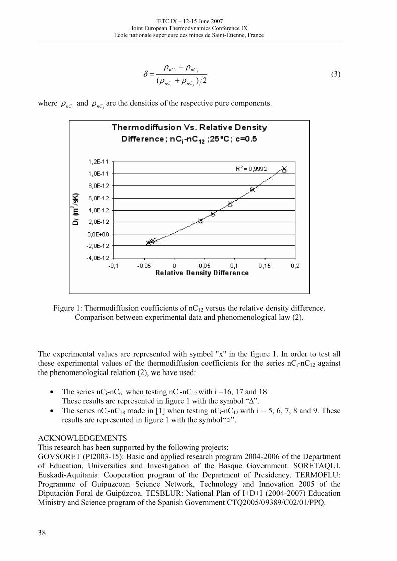
JETC IX – 12-15 June 2007 Joint European Thermodynamics Conference IX
Ecole nationale supérieure des mines de Saint-Étienne, France
38
2)(ji
ji
nCnC
nCnC
ρρρρ
δ+
−= (3)
where
inCρ and jnCρ are the densities of the respective pure components.
Figure 1: Thermodiffusion coefficients of nC12 versus the relative density difference. Comparison between experimental data and phenomenological law (2).
The experimental values are represented with symbol "x" in the figure 1. In order to test all these experimental values of the thermodiffusion coefficients for the series nCi-nC12 against the phenomenological relation (2), we have used:
• The series nCi-nC6 when testing nCi-nC12 with i =16, 17 and 18 These results are represented in figure 1 with the symbol “∆”. • The series nCi-nC18 made in [1] when testing nCi-nC12 with i = 5, 6, 7, 8 and 9. These
results are represented in figure 1 with the symbol“○”. ACKNOWLEDGEMENTS This research has been supported by the following projects: GOVSORET (PI2003-15): Basic and applied research program 2004-2006 of the Department of Education, Universities and Investigation of the Basque Government. SORETAQUI. Euskadi-Aquitania: Cooperation program of the Department of Presidency. TERMOFLU: Programme of Guipuzcoan Science Network, Technology and Innovation 2005 of the Diputación Foral de Guipúzcoa. TESBLUR: National Plan of I+D+I (2004-2007) Education Ministry and Science program of the Spanish Government CTQ2005/09389/C02/01/PPQ.
JETC IX – 12-15 June 2007 Joint European Thermodynamics Conference IX
Ecole nationale supérieure des mines de Saint-Étienne, France
39
Gratefulness for the grant of the Department of Education, Universities and Investigation of the Basque Government. (BFI05.449).
References
[1] Blanco, P.; Bou-Ali, M.; Platten, J.; Madariaga, J.; Urteaga, P. & Santamaría, C., Thermodiffusion coefficient for binary liquid hydrocarbon mixtures, Journal of Non Equilibrium Thermodynamics, 2007, accepted. [2] Clusius, K. & Dickel, G., Kurze Originalmitteilungen, Die Naturwissenschaften, 1938, 27, 148-149. [3] Platten, J.; Bou-Ali, M.; Costesèque, P.; Dutrieux, J.; Köhler, W.; Leppla, C.; Wiegand, S. & G.Wittko, G., Benchmark values for the Soret, thermal diffusion and diffusion coefficients of three binary organic liquid mixtures, Pilosophical Magazine, 2003, 83, 1965-1971. [4] Furry, W.; Jones, R. & Onsager, L., On the Theory of Isotope Separation by Thermal Diffusion, Physical Review E, 1939, 55, 1083-1095. [5] Wittko, G. & Köhler, W., Universal isotope effect in thermal diffusion of mixtures containing cyclohexane and cyclohexane-d12, Journal of Chemical Physics, 2005, 123, 014506-1 - 014506-6. [6] Urteaga, P., Bou-Ali, M. M., Madariaga, J. A., Santamaría, C., Blanco, P., Platten, J. K., Thermogravitational column for high pressure, In M.M. Bou-Ali, J.K. Platten (Ed.), Thermodiffusion: Basics and Applications, Mondragon Unibertsitateko Zerbitzu Editoriala: Mondragon (Spain), 2006, 449-458.
JETC IX – 12-15 June 2007 Joint European Thermodynamics Conference IX
Ecole nationale supérieure des mines de Saint-Étienne, France
40
Determination of liquid/vapour equilibria by ebulliometry and modelling by the quasi ideal model
A.J. Bougrine, E. Labarthe, C. Blanchard, O. Duclos, R. Tenu, H. Delalu, C. Goutaudier
Laboratoire Hydrazines et Procédés, UMR 5179 Université Claude Bernard Lyon 1 – CNRS – Isochem/SNPE
43, Bd du 11 Novembre 1918, 69622 Villeurbanne Cedex, France
[email protected] After the synthesis step, in the laboratory as in the industry, always occurs the question of the isolation of the useful product and often that of the recovery of an expensive reagent. If crystallization and salting-out are processes usually used, distillation is very widely implemented. It indeed allows, by means of tested materials, to obtain simply products of high purity. This study lies in the development of new processes of synthesis, extraction and purification of hydrazine derivatives, molecules of spatial and pharmaceutical interest. In our case, the knowledge of the properties of the liquid/vapour equilibria of the synthesis solutions is then an absolute must. In this aim, we have designed an original ebulliometer working under various range of pressures (0.001-1.5 bar). First, we used two set of tabulated values to certificate our apparatus : the boiling points of water according to the pressure and the equilibrium curves of the methanol-butanol binary system. Secondly, we have determined the liquid/vapour properties for the two following binary diagrams : WaterPiperidine (C5H10NH) and Monochlorobenzene (MCB)CFT Isocyanate. The quasi ideal model, an original model developed by our team, was applied to the predictive calculation of the liquid/vapour equilibria of these systems. This model lies on two fundamental concepts : − the substitution of the probability of existence to the traditional molar fraction which
allows to preserve the Van Laar’s simple formalism of the equations of equilibria between an ideal solution and a perfect gas,
− any fitting parameter devoid of a physical meaning. The general equation used for the modelling is the following :
0 1d Rh
XX
.ln xT
T
i
i
i0i
i
=⎟⎠⎞
⎜⎝⎛⎟
⎠
⎞⎜⎝
⎛ Δ+⎟⎟
⎠
⎞⎜⎜⎝
⎛∫∑ Ti
α
β
By making a systematic study of interactions between constituents, we come to a very good agreement between experimental and calculated values for the MCBCTFI system. However, the modelling is rougher for the C5H10NHH2O binary system, what lets suppose an inadequacy of the hypotheses of the quasi ideal model.
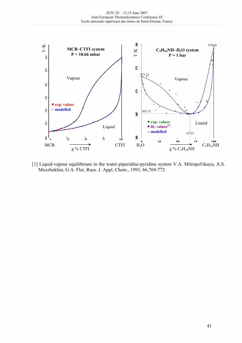
JETC IX – 12-15 June 2007 Joint European Thermodynamics Conference IX
Ecole nationale supérieure des mines de Saint-Étienne, France
41
[1] Liquid-vapour equilibrium in the water-piperidine-pyridine system V.A. Mitropol'skaya, A.S. Mozzhukhin, G.A. Fler, Russ. J. Appl. Chem., 1993, 66,769-772.
MCB−CTFI system P = 18.66 mbar
Vapour
Liquid
exp. values − modelled
T /K
30
3 31
3 32
3 33
3 34
3 35
3 36
3
0 25 50 75 100
g % CTFI MCB CTFI
C5H10NH−H2O system P = 1 bar
Vapour
Liquid exp. values lit. values[1]
− modelled
g % C5H10NH
T /K
379.26
373.15
365.15
67.33
C5H10NH H2O
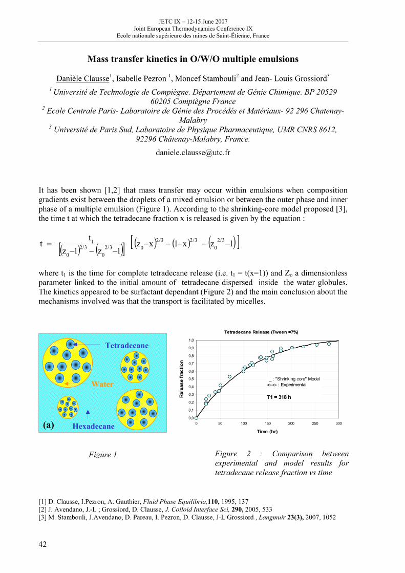
JETC IX – 12-15 June 2007 Joint European Thermodynamics Conference IX
Ecole nationale supérieure des mines de Saint-Étienne, France
42
Mass transfer kinetics in O/W/O multiple emulsions
Danièle Clausse1, Isabelle Pezron 1, Moncef Stambouli2 and Jean- Louis Grossiord3 1 Université de Technologie de Compiègne. Département de Génie Chimique. BP 20529
60205 Compiègne France 2 Ecole Centrale Paris- Laboratoire de Génie des Procédés et Matériaux- 92 296 Chatenay-
Malabry 3 Université de Paris Sud, Laboratoire de Physique Pharmaceutique, UMR CNRS 8612,
92296 Châtenay-Malabry, France.
[email protected] It has been shown [1,2] that mass transfer may occur within emulsions when composition gradients exist between the droplets of a mixed emulsion or between the outer phase and inner phase of a multiple emulsion (Figure 1). According to the shrinking-core model proposed [3], the time t at which the tetradecane fraction x is released is given by the equation :
( ) ( )[ ] ( ) ( ) ( )[ ] 1z x1 xz 1z 1z
t t 3/2
03/23/2
03/20
3/20
1 −−−−−−−−
=
where t1 is the time for complete tetradecane release (i.e. t1 = t(x=1)) and Zo a dimensionless parameter linked to the initial amount of tetradecane dispersed inside the water globules. The kinetics appeared to be surfactant dependant (Figure 2) and the main conclusion about the mechanisms involved was that the transport is facilitated by micelles.
Tetradecane Release (Tween =7%)
0,0
0,1
0,2
0,3
0,4
0,5
0,6
0,7
0,8
0,9
1,0
0 50 100 150 200 250 300
Time (hr)
Rel
ease
frac
tion
__ : "Shrinking core" Model-o--o- : Experimental
T1 = 318 h
[1] D. Clausse, I.Pezron, A. Gauthier, Fluid Phase Equilibria,110, 1995, 137 [2] J. Avendano, J.-L ; Grossiord, D. Clausse, J. Colloid Interface Sci, 290, 2005, 533 [3] M. Stambouli, J.Avendano, D. Pareau, I. Pezron, D. Clausse, J-L Grossiord , Langmuir 23(3), 2007, 1052
Hexadecane
WWaatteerr
Tetradecane
(a)
Figure 1 Figure 2 : Comparison between experimental and model results for tetradecane release fraction vs time
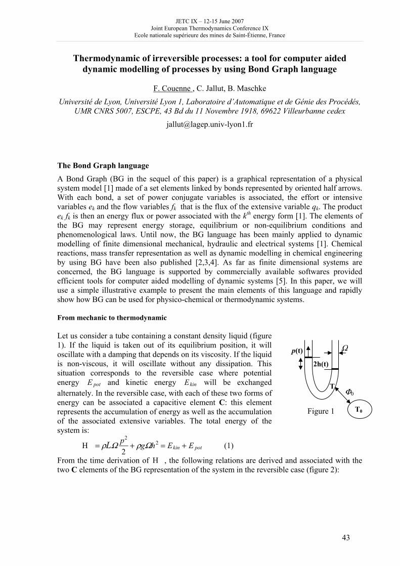
JETC IX – 12-15 June 2007 Joint European Thermodynamics Conference IX
Ecole nationale supérieure des mines de Saint-Étienne, France
43
Thermodynamic of irreversible processes: a tool for computer aided dynamic modelling of processes by using Bond Graph language
F. Couenne , C. Jallut, B. Maschke
Université de Lyon, Université Lyon 1, Laboratoire d’Automatique et de Génie des Procédés, UMR CNRS 5007, ESCPE, 43 Bd du 11 Novembre 1918, 69622 Villeurbanne cedex
The Bond Graph language
A Bond Graph (BG in the sequel of this paper) is a graphical representation of a physical system model [1] made of a set elements linked by bonds represented by oriented half arrows. With each bond, a set of power conjugate variables is associated, the effort or intensive variables ek and the flow variables fk that is the flux of the extensive variable qk. The product ek fk is then an energy flux or power associated with the kth energy form [1]. The elements of the BG may represent energy storage, equilibrium or non-equilibrium conditions and phenomenological laws. Until now, the BG language has been mainly applied to dynamic modelling of finite dimensional mechanical, hydraulic and electrical systems [1]. Chemical reactions, mass transfer representation as well as dynamic modelling in chemical engineering by using BG have been also published [2,3,4]. As far as finite dimensional systems are concerned, the BG language is supported by commercially available softwares provided efficient tools for computer aided modelling of dynamic systems [5]. In this paper, we will use a simple illustrative example to present the main elements of this language and rapidly show how BG can be used for physico-chemical or thermodynamic systems. From mechanic to thermodynamic Let us consider a tube containing a constant density liquid (figure 1). If the liquid is taken out of its equilibrium position, it will oscillate with a damping that depends on its viscosity. If the liquid is non-viscous, it will oscillate without any dissipation. This situation corresponds to the reversible case where potential energy E pot and kinetic energy Ekin will be exchanged alternately. In the reversible case, with each of these two forms of energy can be associated a capacitive element C: this element represents the accumulation of energy as well as the accumulation of the associated extensive variables. The total energy of the system is:
H = ρLΩ p2
2+ ρgΩh2 = Ekin + E pot (1)
From the time derivation of H , the following relations are derived and associated with the two C elements of the BG representation of the system in the reversible case (figure 2):
Figure 1
Φ0 T
2h(t)
p(t) Ω
T0
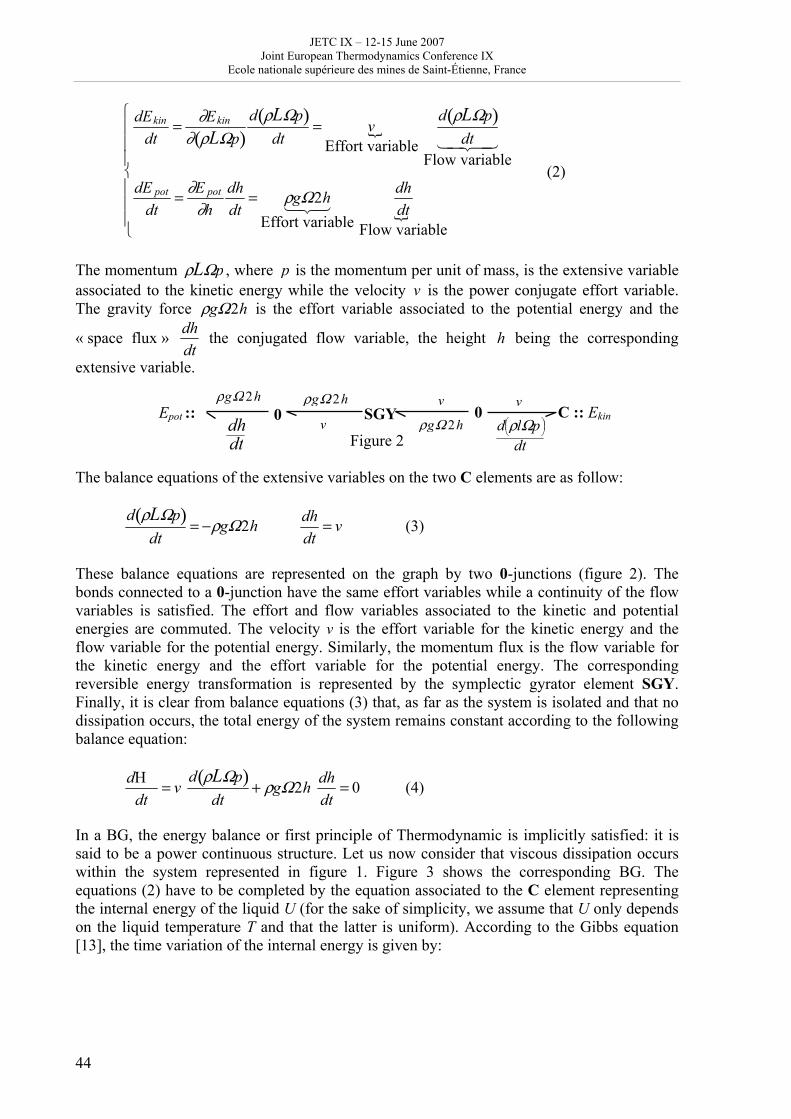
JETC IX – 12-15 June 2007 Joint European Thermodynamics Conference IX
Ecole nationale supérieure des mines de Saint-Étienne, France
44
dEkin
dt= ∂Ekin
∂ ρLΩp( )d ρLΩp( )
dt= v
Effort variable{
d ρLΩp( )dt
Flow variable1 2 4 3 4
dE pot
dt= ∂E pot
∂hdhdt
= ρgΩ2hEffort variable
1 2 3 dhdt
Flow variable{
⎧
⎨
⎪ ⎪ ⎪
⎩
⎪ ⎪ ⎪
(2)
The momentum ρLΩp , where p is the momentum per unit of mass, is the extensive variable associated to the kinetic energy while the velocity v is the power conjugate effort variable. The gravity force ρgΩ2h is the effort variable associated to the potential energy and the
« space flux » dhdt
the conjugated flow variable, the height h being the corresponding
extensive variable.
Figure 2
The balance equations of the extensive variables on the two C elements are as follow:
d ρLΩp( )
dt= −ρgΩ2h dh
dt= v (3)
These balance equations are represented on the graph by two 0-junctions (figure 2). The bonds connected to a 0-junction have the same effort variables while a continuity of the flow variables is satisfied. The effort and flow variables associated to the kinetic and potential energies are commuted. The velocity v is the effort variable for the kinetic energy and the flow variable for the potential energy. Similarly, the momentum flux is the flow variable for the kinetic energy and the effort variable for the potential energy. The corresponding reversible energy transformation is represented by the symplectic gyrator element SGY. Finally, it is clear from balance equations (3) that, as far as the system is isolated and that no dissipation occurs, the total energy of the system remains constant according to the following balance equation:
dH
dt= v
d ρLΩp( )dt
+ ρgΩ2h dhdt
= 0 (4)
In a BG, the energy balance or first principle of Thermodynamic is implicitly satisfied: it is said to be a power continuous structure. Let us now consider that viscous dissipation occurs within the system represented in figure 1. Figure 3 shows the corresponding BG. The equations (2) have to be completed by the equation associated to the C element representing the internal energy of the liquid U (for the sake of simplicity, we assume that U only depends on the liquid temperature T and that the latter is uniform). According to the Gibbs equation [13], the time variation of the internal energy is given by:
C :: Ekin 0 v
d ρlΩp⎛ ⎝ ⎜ ⎞
⎠ ⎟
dt
Epot :: 0 dhdt
SGYρgΩ 2hv
v ρgΩ 2hρgΩ 2h
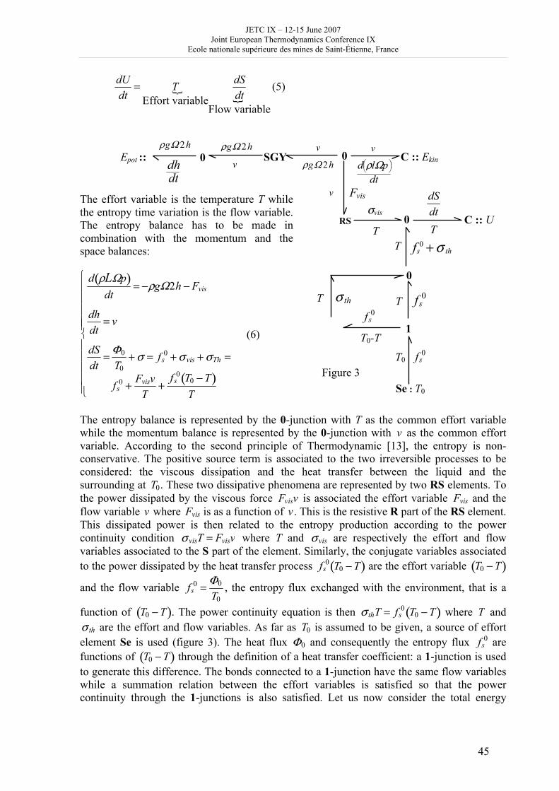
JETC IX – 12-15 June 2007 Joint European Thermodynamics Conference IX
Ecole nationale supérieure des mines de Saint-Étienne, France
45
dUdt
= TEffort variable
{dSdt
Flow variable{
(5)
The effort variable is the temperature T while the entropy time variation is the flow variable. The entropy balance has to be made in combination with the momentum and the space balances:
d ρLΩp( )dt
= −ρgΩ2h − Fvis
dhdt
= v
dSdt
= Φ0
T0+ σ = fs
0 + σ vis + σTh =
fs0 + Fvisv
T+
fs0 T0 − T( )
T
⎧
⎨
⎪ ⎪ ⎪ ⎪ ⎪
⎩
⎪ ⎪ ⎪ ⎪ ⎪
(6)
The entropy balance is represented by the 0-junction with T as the common effort variable while the momentum balance is represented by the 0-junction with v as the common effort variable. According to the second principle of Thermodynamic [13], the entropy is non-conservative. The positive source term is associated to the two irreversible processes to be considered: the viscous dissipation and the heat transfer between the liquid and the surrounding at T0. These two dissipative phenomena are represented by two RS elements. To the power dissipated by the viscous force Fvisv is associated the effort variable Fvis and the flow variable v where Fvis is as a function of v . This is the resistive R part of the RS element. This dissipated power is then related to the entropy production according to the power continuity condition σ visT = Fvisv where T and σ vis are respectively the effort and flow variables associated to the S part of the element. Similarly, the conjugate variables associated to the power dissipated by the heat transfer process fs
0 T0 − T( ) are the effort variable T0 − T( )
and the flow variable fs0 = Φ0
T0, the entropy flux exchanged with the environment, that is a
function of T0 − T( ). The power continuity equation is then σ thT = fs0 T0 − T( ) where T and
σ th are the effort and flow variables. As far as T0 is assumed to be given, a source of effort element Se is used (figure 3). The heat flux Φ0 and consequently the entropy flux fs
0 are functions of T0 − T( ) through the definition of a heat transfer coefficient: a 1-junction is used to generate this difference. The bonds connected to a 1-junction have the same flow variables while a summation relation between the effort variables is satisfied so that the power continuity through the 1-junctions is also satisfied. Let us now consider the total energy
C :: Ekin 0 v
d ρlΩp⎛ ⎝ ⎜ ⎞
⎠ ⎟
dt
SGYEpot :: 0 dhdt
ρgΩ 2hv
v ρgΩ 2hρgΩ 2h
v
RS
Fvis
fs0 + σ thT
T C :: U 0
σvis
dSdtT
T
Se : T0
1 T0-T
0
T fs0σ th
T0
fs0
fs0
Figure 3
JETC IX – 12-15 June 2007 Joint European Thermodynamics Conference IX
Ecole nationale supérieure des mines de Saint-Étienne, France
46
associated to the BG in figure 3, E = ρLΩ p2
2+ ρgΩh2 + U . Its time derivative is given
according to the balance equations (6):
dEdt
= v d ρLΩp( )
dt+ ρgΩ2h dh
dt+ T dS
dt=Φ0 (7)
The first principle remains implicitly satisfied. Conclusion: extension to physico-chemical or thermodynamic systems If the total energy of a system can be reduced to its internal energy, the Gibbs equation is the basis for such an extension [6]:
dUdt
= T dSdt
− P dVdt
+ μidNi
dti∑ (8)
A balance equation has to be written for each extensive variable, the entropy S, the space or volume V and the number of mole of component i, Ni [4]. The entropy production will include the irreversible phenomena due chemical reactions as well as heat and mass transfer. Furthermore, infinite dimensional systems (those represented by partial differential equations) can also be represented through such concepts since the Gibbs equation (8) is valid for specific quantities and for substantial derivatives [6]:
DuDt
= T DsDt
− P DvDt
+ μiDxi
Dti∑ (9)
List of references [1] D. Karnopp, D. Margolis and R. Rosenberg, Systems Dynamics a Unified Approach. John Wiley and Sons, New York, 2000 [2] H. Atlan, A. Katzir-Katchalsky, Tellegen’s theorem for bong-graphs. Its relevance to chemical networks, Currents in Modern Biology, 5 (1973), 55 [2] G. F. Oster, A. S. Perelson, A. Katchalsky, Network thermodynamic: dynamic modelling of biophysical systems, Quarterly Reviews in Biophysics 6(I) (1973), 1 [3] A. M. Simon, P. Doran, R. Paterson, Assessment of diffusion coupling effects in membrane separation. Part I. Network thermodynamics modelling, Journal of Membrane Science, 109(2) (1996), 231 [4] F. Couenne, C. Jallut, B. Maschke, P. C. Breedveld, M. Tayakout, Bond graph modelling for chemical reactors, Mathematical and Computer Modelling of Dynamical Systems, 12(2-3) (2006), 159 [5] http://www.bondgraphs.com/software.html [6] S. R. De Groot and P. Mazur, Non-equilibrium thermodynamics, Dover, 1984
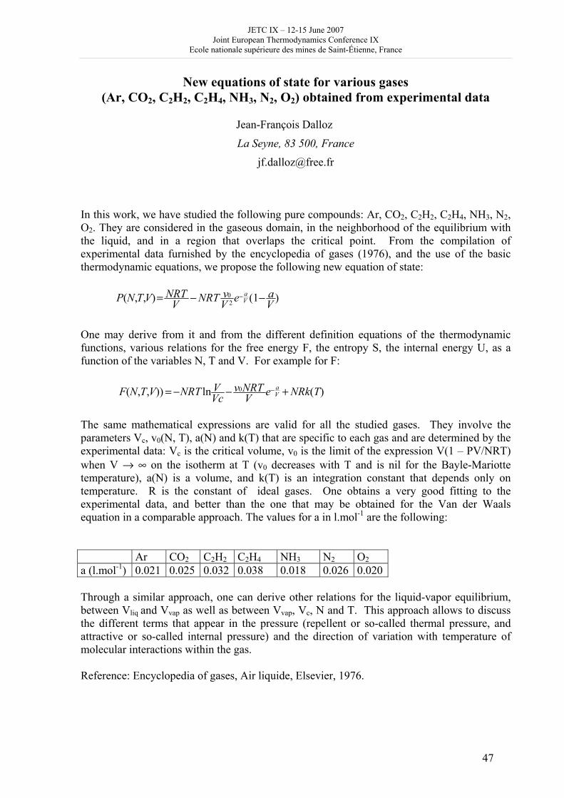
JETC IX – 12-15 June 2007 Joint European Thermodynamics Conference IX
Ecole nationale supérieure des mines de Saint-Étienne, France
47
New equations of state for various gases (Ar, CO2, C2H2, C2H4, NH3, N2, O2) obtained from experimental data
Jean-François Dalloz
La Seyne, 83 500, France
[email protected] In this work, we have studied the following pure compounds: Ar, CO2, C2H2, C2H4, NH3, N2, O2. They are considered in the gaseous domain, in the neighborhood of the equilibrium with the liquid, and in a region that overlaps the critical point. From the compilation of experimental data furnished by the encyclopedia of gases (1976), and the use of the basic thermodynamic equations, we propose the following new equation of state: )1(),,( 2
0VaeV
vNRTVNRTVTNP V
a −−= −
One may derive from it and from the different definition equations of the thermodynamic functions, various relations for the free energy F, the entropy S, the internal energy U, as a function of the variables N, T and V. For example for F: )(ln)),,( 0 TNRkeV
NRTvVcVNRTVTNF V
a +−−= −
The same mathematical expressions are valid for all the studied gases. They involve the parameters Vc, v0(N, T), a(N) and k(T) that are specific to each gas and are determined by the experimental data: Vc is the critical volume, v0 is the limit of the expression V(1 – PV/NRT) when V → ∞ on the isotherm at T (v0 decreases with T and is nil for the Bayle-Mariotte temperature), a(N) is a volume, and k(T) is an integration constant that depends only on temperature. R is the constant of ideal gases. One obtains a very good fitting to the experimental data, and better than the one that may be obtained for the Van der Waals equation in a comparable approach. The values for a in l.mol-1 are the following: Ar CO2 C2H2 C2H4 NH3 N2 O2 a (l.mol-1) 0.021 0.025 0.032 0.038 0.018 0.026 0.020 Through a similar approach, one can derive other relations for the liquid-vapor equilibrium, between Vliq and Vvap as well as between Vvap, Vc, N and T. This approach allows to discuss the different terms that appear in the pressure (repellent or so-called thermal pressure, and attractive or so-called internal pressure) and the direction of variation with temperature of molecular interactions within the gas. Reference: Encyclopedia of gases, Air liquide, Elsevier, 1976.
JETC IX – 12-15 June 2007 Joint European Thermodynamics Conference IX
Ecole nationale supérieure des mines de Saint-Étienne, France
48
The controversy between Boltzmann and Ostwald
François-Xavier Demoures
Ecole Normale Supérieure Lettres et Sciences Humaines (Lyon) department of Philosophy
[email protected] The arrow of time presents an enormous challenge to philosophy of science. Can we deal with the structure of time without taking into account the evolution of phenomena? Can we think equally time and evolution, or can we share on the one hand the time structure – the time flow – and on the other hand the time arrow? Isabelle Stengers writes : “The time arrow is not problematic : it is obvious.” According to Ostwald, “time properties are so simple and obvious that no science deals with them.” Behind this evidence, I will try to explain why, or at least, why one part of this problem has not been solved until now. In my opinion, the root of this problem can be identified in the controversy opposing Boltzmann and Ostwald about the hypothesis of molecular collision and the mathematical models that Boltzmann used to establish the bases of gas kinetics and statistical mechanics. Ostwald did not accept molecular models and tried to contest the hegemonic position of Lagrange’s Rational Mechanics. He criticized Boltzmann for using reversible equations in order to describe an irreversible phenomena. Consequently he seemed to contest the results of experience and to contradict reality. The problem was triple. Firstly, Ostwald opposed to Boltzmann an other theory of knowledge, based on Mach’s epistemology. According to him, an hypothetico-deductive process was not compatible with a serious science which pretended to give an account of the structure of the World. The only possible scientific method was induction and measure, whereas Boltzmann preferred assumptions and efficient mathematical models. Secondly, it was precisely a mathematical problem, more exactly the status of mathematical models in physics. Could a model be in contradiction with obvious experience? Could we use discrete models to deal with a continuous phenomena ? Third we can emphasize the difference of laboratory practices between a chemist as Oswtald and a physicist as Boltzmann. The Ostwald’s conception of science was still a conception that belonged to past, however he was a big chemist. He did not see the turning point of theoretical chemistry and theoretical physics that Boltzmann represented. Boltzmann went from a correspondentist system of language to a coherentist system, and that is the philosophical revolution made by his theories. So the question is essentially a philosophical problem of language and logics since incomprehension can be explained with opposed language games (Wittgenstein). For the moment I propose to distinguish time structure and time arrow, in order to prevent from confusions. Keywords : history of science, time, time arrow, Boltzmann, Ostwald, Duhem, atomist model, energetism
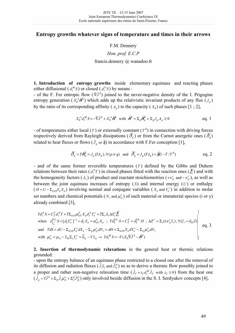
JETC IX – 12-15 June 2007 Joint European Thermodynamics Conference IX
Ecole nationale supérieure des mines de Saint-Étienne, France
49
Entropy growths whatever signs of temperature and times in their arrows
F.M. Dennery
Hon. prof. E.C.P
francis.dennery @ wanadoo.fr 1. Introduction of entropy growths inside elementary equimass and reacting phases either diffusional ( dt
M S ) or closed ( dtN S ) by means :
- of the F. Fer entropic flow ( r ∇
r J S) joined to the never-negative density of the I. Prigogine
entropy generation ( X0−1 Ý σ S ) which adds up the relativistic invariant products of any flux ( J p )
by the ratio of its corresponding affinity ( Ap ) to the capacity ( X0 ) of such phases [1 ; 2], X0
−1dtM S = −
r ∇
r J S + X0
−1 Ý σ S with Ý σ S = Σ p Ý σ pS = Σ pJ p Ap ≥ 0 eq. 1
- of temperatures either local (T ) or externally constant (T 0) in connection with driving forces respectively derived from Rayleigh dissipations ( Ý D p ) or from the Carnot anergetic ones ( Ý D q ) related to heat fluxes or flows ( J q or Ýq ) in accordance with F.Fer conception [1], Ý D p = T Ý σ p
S = J p (TAp ) ,∀(p ≠ q) and Ý D q = Jq (TAq ) = Ý q (1−T /T 0) eq. 2 - and of the same former reversible temperatures (T ) defined by the Gibbs and Duhem relations between their rates ( dt
NT ) in closed phases fitted with the reaction ones ( Ý ξ r ) and with the homogeneity factors ( λr) of product and reactant stoichiometries ( +ν iy
r and − ν iyr ), as well as
between the joint equimass increases of entropy ( S) and internal energy (U ) or enthalpy ( H = U − Σn≥0Yn Xn ) involving normal and conjugate variables ( Xn and Yn
= ) in addition to molar set numbers and chemical potentials ( N i and μ iy
= ) of each material or immaterial species (i or y) already combined [3],
TdtN S = CT
Y dtNT +TΣn≥0αnT
Y XndtNYn
= +TΣrλrΔSs= Ý ξ r
when ∂Yn
=TNi S = [∂SYn
= ]−1 = ∂T Xn = αnTY Xn ; T∂T
YNi S = CTY = ∂T
YNi H ; ΔZ= = Σ i (±ν iyr z i) , ∀(z i = ∂NiZ)
and TdS = dU − Σn≥0Yn= dXn − Σiyμ iy
= dN i = dH + Σn≥0XndYn= − Σiyμ iy
= dN i
with μ iy= = μxi − x 0iΣyYy
= = h iy −T s xi → TdtM S = −T (X0
r ∇
r J S − Ý σ S )
⎤
⎦
⎥ ⎥ ⎥ ⎥ ⎥ ⎥
eq. 3
2. Insertion of thermodynamic relaxations in the general heat or thermic relations grounded: - upon the entropy balance of an equimass phase restricted to a closed one after the removal of its diffusion and radiation fluxes (
r J is i and
r J sy
ρ ) so as to derive a thermic flow possibly joined to a proper and rather non-negative relaxation time (
r J T + tT dt
M r J T with tT ≥ 0) from the heat one
(
r J q = T
r J S + Σ iy
r J iμ iy
= + Σyρ r
J fyρ ) only involved beside diffusion in the S. I. Serdyukov concepts [4],
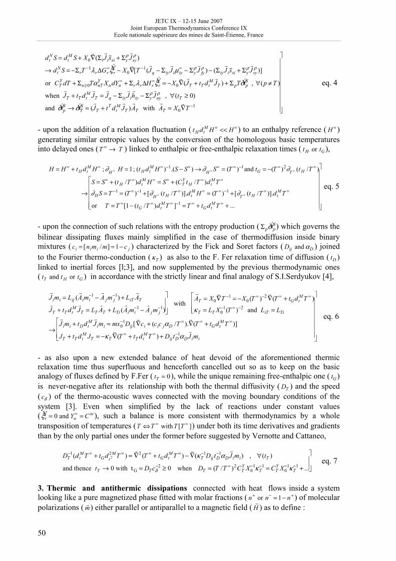
JETC IX – 12-15 June 2007 Joint European Thermodynamics Conference IX
Ecole nationale supérieure des mines de Saint-Étienne, France
50
dtN S = dt
M S + X0r ∇ (Σi
r J is xi + Σy
ρ r J sy
ρ )
→ dtN S = −ΣrT
−1λrΔGr= Ý ξ r − X0
r ∇ [T −1(
r J q − Σiy
r J iμ iy
= − Σyρ r J fy
ρ ) − (Σiy
r J is xi + Σy
ρ r J sy
ρ )]
or CTY dT + Σn≥0TαnT
Y XndYn= + ΣrλrΔHr
= Ý ξ r = −X0r ∇ (
r J T + tT dt
M r J T ) + Σ pT Ý σ p
S , ∀(p ≠ T )
whenr J T + tT dt
M r J T =
r J q − Σ iy
r J i
r h iy − Σy
ρ r J uy
ρ , ∀(tT ≥ 0)
and Ý σ pS → Ý σ T
S = (r J T + tT dt
M r J T )
r A T with
r A T = X0
r ∇ T −1
⎤
⎦
⎥ ⎥ ⎥ ⎥ ⎥ ⎥ ⎥ ⎥
eq. 4
- upon the addition of a relaxation fluctuation ( t H dt
M H = << H = ) to an enthalpy reference ( H = ) generating similar entropic values by the conversion of the homologous basic temperatures into delayed ones (T = → T ) linked to enthalpic or free-enthalpic relaxation times ( t H or tG),
H = H = + t H dtM H = ;∂H = H = 1; (t H dt
M H = )−1.(S − S= ) → ∂H = S= = (T = )−1and tG = −(T = )2∂T = (t H /T = )
→
S = S= + (t H /T = )dtM H = = S= + (CT
Y t H /T = )dtM T =
∂H S = T −1 = (T = )−1 + [∂H = (t H /T = )].dtM H = = (T = )−1 + [∂T = (t H /T = )].dt
M T =
or T = T =[1− (tG /T = )dtM T = ]−1 = T = + tGdt
M T = + ...
⎡
⎣
⎢ ⎢ ⎢ ⎢
⎤
⎦
⎥ ⎥ ⎥ ⎥ ⎥ ⎥
eq. 5
- upon the connection of such relations with the entropy production ( Σ p Ý σ p
S) which governs the bilinear dissipating fluxes mainly simplified in the case of thermodiffusion inside binary mixtures ( ci = [nimi /m] = 1− c j ) characterized by the Fick and Soret factors ( Dij and αD ) joined to the Fourier thermo-conduction (κT ) as also to the F. Fer relaxation time of diffusion ( tD ) linked to inertial forces [l;3], and now supplemented by the previous thermodynamic ones ( tT and t H or tG ) in accordance with the strictly linear and final analogy of S.I.Serdyukov [4],
r J imi = Lij (
r A imi
−1 −r A jm j
−1) + LiT
r A T
r J T + tT dt
M r J T = LT
r A T + LTi (
r A imi
−1 −r A jm j
−1)
⎤
⎦ ⎥ ⎥
with
r A T = X0
r ∇ T −1 = −X0 (T = )−2 r
∇ (T = + tGdtM T = )
κT = LT X0−1(T = )−2 and LiT = LTi
⎡
⎣ ⎢ ⎢
→
r J imi + tDdt
M r J imi = mx0
−1Dij[r ∇ ci + (cic jαD /T = ).
r ∇ (T = + tGdt
M T = )]
JT + tT dtM JT = −κT
r ∇ (T = + tT dt
M T = ) + Dij tD−1αD
r J imi
⎡
⎣ ⎢ ⎢
⎤
⎦
⎥ ⎥ ⎥ ⎥ ⎥ ⎥
eq. 6
- as also upon a new extended balance of heat devoid of the aforementioned thermic relaxation time thus superfluous and henceforth cancelled out so as to keep on the basic analogy of fluxes defined by F.Fer ( tT = 0), while the unique remaining free-enthalpic one ( tG) is never-negative after its relationship with both the thermal diffusivity ( DT ) and the speed ( cδ ) of the thermo-acoustic waves connected with the moving boundary conditions of the system [3]. Even when simplified by the lack of reactions under constant values ( Ý ξ r = 0 and Yn
= = C te ), such a balance is more consistent with thermodynamics by a whole transposition of temperatures (T ⇔T = with T [T = ]) under both its time derivatives and gradients than by the only partial ones under the former before suggested by Vernotte and Cattaneo,
DT−1(dt
M T = + tGdt 22M T = ) =
r ∇ 2 (T = + tGdt
M T = ) −r ∇ (κT
−1Dij tD−1αD
r J imi) , ∀(tT )
and thence tT → 0 with t G = DT cδ−2 ≥ 0 when DT = (T /T = )2CT
Y X0−1κT
−1 = CTY X0
−1κT−1 + ...
⎤
⎦ ⎥ ⎥ eq. 7
3. Thermic and antithermic dissipations connected with heat flows inside a system looking like a pure magnetized phase fitted with molar fractions ( n+ or n− = 1− n+) of molecular polarizations ( r m ) either parallel or antiparallel to a magnetic field (
r H ) as to define :
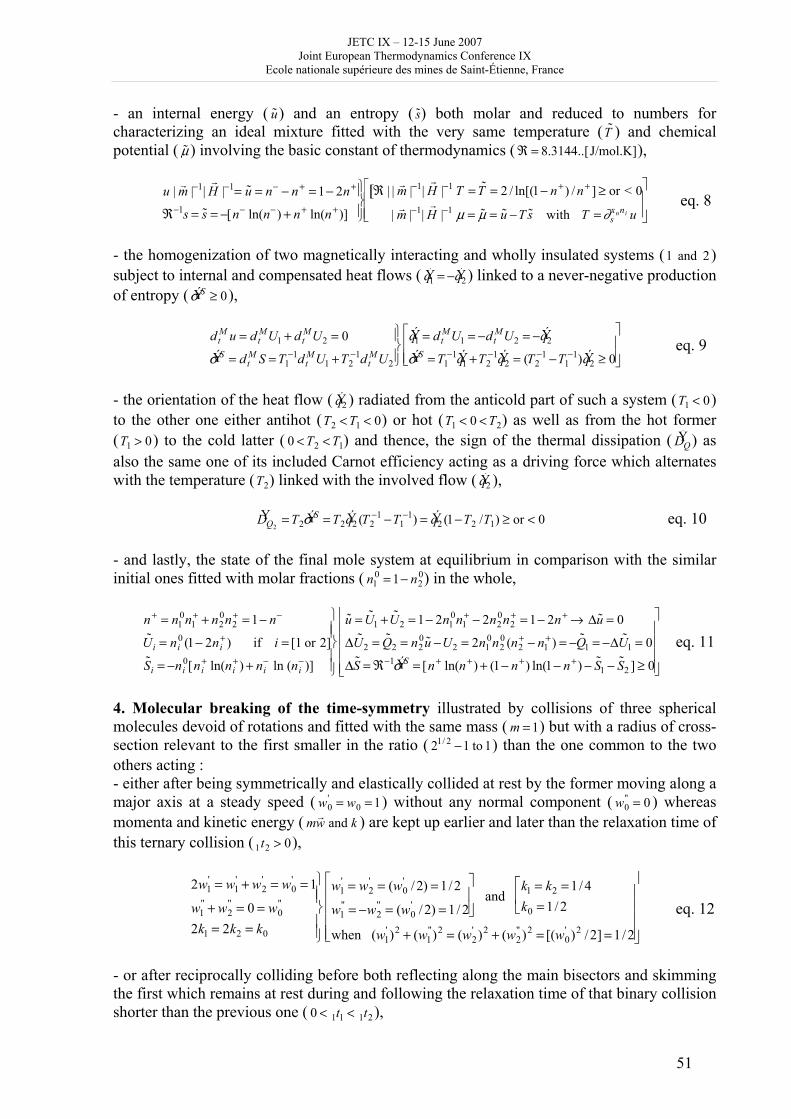
JETC IX – 12-15 June 2007 Joint European Thermodynamics Conference IX
Ecole nationale supérieure des mines de Saint-Étienne, France
51
- an internal energy ( ˜ u ) and an entropy ( ˜ s ) both molar and reduced to numbers for characterizing an ideal mixture fitted with the very same temperature ( ˜ T ) and chemical potential ( ˜ μ ) involving the basic constant of thermodynamics ( ℜ = 8.3144..[J/mol.K]),
u | r m |−1|r
H |−1= ˜ u = n− − n+ = 1− 2n+
ℜ−1s = ˜ s = −[n− ln(n−) + n+ ln(n+)]
⎫ ⎬ ⎪
⎭ ⎪ ℜ |[ | r m |−1|
r H |−1 T = ˜ T = 2 / ln[(1− n+ ) /n+ ] ≥ or < 0
| r m |−1|r
H |−1 μ = ˜ μ = ˜ u −T ˜ s with T = ∂sxnni u
⎡
⎣ ⎢ ⎢
⎤
⎦ ⎥ ⎥ eq. 8
- the homogenization of two magnetically interacting and wholly insulated systems (1 and 2) subject to internal and compensated heat flows ( Ý q 1 = − Ý q 2 ) linked to a never-negative production of entropy ( Ý σ S ≥ 0),
dtM u = dt
M U1 + dtM U2 = 0
Ý σ S = dtM S = T1
−1dtM U1 +T2
−1dtM U2
⎫ ⎬ ⎪
⎭ ⎪
Ý q 1 = dtM U1 = −dt
M U2 = − Ý q 2Ý σ S = T1
−1 Ý q 1 +T2−1 Ý q 2 = (T2
−1 −T1−1) Ý q 2 ≥ 0
⎡
⎣ ⎢ ⎢
⎤
⎦ ⎥ ⎥ eq. 9
- the orientation of the heat flow ( Ý q 2 ) radiated from the anticold part of such a system (T1 < 0) to the other one either antihot (T2 < T1 < 0) or hot (T1 < 0 < T2) as well as from the hot former (T1 > 0) to the cold latter ( 0 < T2 < T1) and thence, the sign of the thermal dissipation ( Ý D Q) as also the same one of its included Carnot efficiency acting as a driving force which alternates with the temperature (T2) linked with the involved flow ( Ý q 2 ), Ý D Q2
= T2 Ý σ S = T2 Ý q 2 (T2−1 −T1
−1) = Ý q 2 (1−T2 /T1) ≥ or < 0 eq. 10 - and lastly, the state of the final mole system at equilibrium in comparison with the similar initial ones fitted with molar fractions ( n1
0 = 1− n20) in the whole,
n+ = n1
0n1+ + n2
0n2+ = 1− n−
˜ U i = ni0 (1− 2ni
+ ) if i = [1 or 2]˜ S i = −ni
0[ni+ ln(ni
+) + ni− ln (ni
−)]
⎫
⎬ ⎪ ⎪
⎭ ⎪ ⎪
˜ u = ˜ U 1 + ˜ U 2 = 1− 2n10n1
+ − 2n20n2
+ = 1− 2n+ → Δ ˜ u = 0
Δ ˜ U 2 = ˜ Q 2 = n20 ˜ u −U2 = 2n1
0n20 (n2
+ − n1+) = − ˜ Q 1 = −Δ ˜ U 1 = 0
Δ ˜ S = ℜ−1 Ý σ S = [n+ ln(n+) + (1− n+) ln(1− n+) − ˜ S 1 − ˜ S 2 ] ≥ 0
⎤
⎦
⎥ ⎥ ⎥ ⎥
⎡
⎣
⎢ ⎢ ⎢ ⎢
eq. 11
4. Molecular breaking of the time-symmetry illustrated by collisions of three spherical molecules devoid of rotations and fitted with the same mass ( m = 1) but with a radius of cross-section relevant to the first smaller in the ratio ( 21/ 2 −1 to 1) than the one common to the two others acting : - either after being symmetrically and elastically collided at rest by the former moving along a major axis at a steady speed ( w0
' = w0 = 1) without any normal component ( w0" = 0 ) whereas
momenta and kinetic energy ( mr w and k ) are kept up earlier and later than the relaxation time of
this ternary collision (1t2 > 0),
2w1
' = w1' + w2
' = w0' = 1
w1" + w2
" = 0 = w0"
2k1 = 2k2 = k0
⎫
⎬ ⎪ ⎪
⎭ ⎪ ⎪
w1' = w2
' = (w0' / 2) = 1/2
w1" = −w2
" = (w0' / 2) = 1/2
⎤
⎦ ⎥ ⎥
andk1 = k2 = 1/4k0 = 1/2⎡
⎣ ⎢
when (w1' )2 + (w1
")2 = (w2' )2 + (w2
" )2 = [(w0' )2 / 2] = 1/2
⎡
⎣
⎢ ⎢ ⎢ ⎢
⎤
⎦
⎥ ⎥ ⎥ ⎥
eq. 12
- or after reciprocally colliding before both reflecting along the main bisectors and skimming the first which remains at rest during and following the relaxation time of that binary collision shorter than the previous one ( 0 < 1t1 < 1t2),
JETC IX – 12-15 June 2007 Joint European Thermodynamics Conference IX
Ecole nationale supérieure des mines de Saint-Étienne, France
52
w1' = w2
' → −1/2 ; w1" = −w2
" → −1/2 ; w0' → w0
" = 0 with k1 = k2 → 1/4 when k0 = 0 eq. 13 - and in any case, as one among the three fermions belonging to a molar set of similar configurations inside a phase at rest which keeps up its internal energy (U ) adding together the kinetic and elastic ones between and during collisions in the lack of other interactions ( k1 + k2 = k0 → U = C.te); such conditions are sufficient for breaking the time-symmetry since configurations either single ( Ω III
' = 1) before the previous ternary collisions or double ( Ω II' = 2)
before binary ones at their corresponding times ( tIII' or tII
' ), are ever paired ( Ω III" = Ω II
" = 2) after them ( tIII
" = tIII' +1t2 or tII
" = tII' +1t1).
Thence the reduced entropy ( ˜ S = lnΩ) is increased in the former case ( Δ ˜ S III = ln[2 /1] ≥ 0) but remains constant in the latter ( Δ ˜ S II = ln[1/1] = 0) both occuring with respective mole numbers ( NIII or NII ) during the aforementioned time lags (1t2 or 1t1) in accordance with the T. Petrovsky and I. Prigogine entropy production ( Ý σ III
S ≥ 0) extending Boltzmann conceptions devoid of it ( Ý σ II
S = 0) but consistent with equilibria of systems either largely expanded ( N III → 0) or composed of massless particles, contrary to the unceasingly dissipating molecular ones [5],
Ý σ IIIS dt = NIII ℜΔ ˜ S III = NIII ℜ ln(2) > 0 and Ý σ II
S dt = N IIt II
'
t II"
∫t' III
t" III
∫ ℜΔ ˜ S II = NII ℜ ln(1) = 0 eq. 14
5. Inferences from entropy growths adding up fluxes and production : - by the free-enthalpic relaxation time of S.I.Serdyukov converting Gibbs and Duhem basic temperatures into delayed ones henceforth involved both in affinities and dissipations or even in fluxes included in the last extended balances of entropy and heat [3 ; 4], - by the invariant relativistic and never-negative density of entropy production governing ever since heat flows between partial systems fitted with positive and negative temperatures [3 ; 6], - and by the time-symmetry broken by ternary collisions of mass molecules supplied by the entropic granulation of energy appearing with the big-bang of our Universe and disappearing after its furthermost dematerialization, so that the maximum of entropy production thus reached between them generates physical and chemical or biological dissipating structures among the most elaborate beings after T.Petrovsky and I.Prigogine beside S.Hawking [5 ; 7]. Bibliography [l] Fer F., Thermodynamique macroscopique, Paris, Gordon & Breach, (1970/71). [2] Glansdorff P., Prigogine I., Structure, stabilité et fluctuations, Paris, Masson, (1971). [3] Dennery F.M., "New characterization of propagations in thermodiffusion", Thermodiffusion: Basics & Applications, San Sebastian, Mondragon Unibertsitatea, (2006). [4] Serdyukov S.I., "Extended thermodynamics of irreversible processes predicts a new type of thermodiffusion", Thermodiffusion : Basics & App1ications, San Sebastian, Mondragon Unibertsitatea, (2006). [5] Petrovsky T., Prigogine I. "Quantum chaos, complex spectral representation and time-symmetry breaking". Chaos, Solitons and Fractals, vol. 4, n° 3 (1994), 311-359. [6] Ngô H. and C., Physique statistique, Paris, Masson, (1988). [7] Hawking S., A brief history of time from the big-bang to black holes, New York, Bantam, (1988).
JETC IX – 12-15 June 2007 Joint European Thermodynamics Conference IX
Ecole nationale supérieure des mines de Saint-Étienne, France
53
Waiting for Carnot, some reflections on thermodynamics and complex systems
Prof.em.dr.ir. J. de Swaan Arons
Delft University of Technology Delft, The Netherlands
and Royal Dutch Shell Chair
Chemical Engineering Dept. Tsinghua University
Beijing, China
[email protected] “Why are things becoming more complex?” asked Stanford economist W. Brian Stuart in an essay in the Scientific American. And in a popular book about “Complexity”, Michael Waldrup gave one of the final chapters the title “Waiting for Carnot”. So is there, possibly, a relation between thermodynamics and complexity? After having introduced the concepts of “out of equilibrium with the environment” and “dissipative structures and their maintenance” we will address the question of what has driven living systems to become the most complex chemical factories. It will be shown that “phase” transitions from one non-equilibrium state to another and self-organization are likely to have been prominent phenomena in the original design of these “factories”. It is argued that the driving force behind this design and its complexity is largely to be found in thermodynamic concepts. It may well require somebody of the stature of Sadi Carnot to formulate such a principle in a new universal law. Acknowledgement The author wishes to acknowledge the great inspiration he has experienced during his full working life from the ideas of Ilya Prigogine and his school.
JETC IX – 12-15 June 2007 Joint European Thermodynamics Conference IX
Ecole nationale supérieure des mines de Saint-Étienne, France
54
Reversible computers
Alexis De Vos and Yvan Van Rentergem
Imec v.z.w. and Universiteit Gent Sint-Pietersnieuwstraat 41, B-9000 Gent, Belgium
[email protected] Introduction
Reversible computing [1] is useful both in lossless classical computing [2][3] and in quantum computing [4]. It can be implemented in both classical and quantum hardware technologies.
Reversible logic circuits distinguish themselves from arbitrary logic circuits by two properties: (1) the number of output bits equals the number of input bits and (2) for each pair of different input words, the two corresponding output words are different. For instance, it is clear that an AND gate is not reversible, as (a) it has only one output bit, but two input bits and (b) for three different input words, the output words are equal. See Table 1a. On the other hand, Table 1b gives an example of a reversible truth table. Here, the number of inputs equals the number of outputs, i.e. three. This number is called the width w of the reversible circuit. The table gives all possible input words ABC. We see how all the corresponding output words PQR are different. Implementation For physical implementation, dual logic is very convenient. It means that any logic variable X is represented by two physical quantities, the former representing X itself, the latter representing NOT X. Thus, e.g. the physical gate realizing the logic gate of Table 1b has six physical inputs: A, NOT A, B, NOT B, C, and NOT C, or, in short-hand notation: A, A , B,
B , C, and C . It also has six physical outputs: P, P , Q, Q , R , and R . Such approach is common in electronics, where it is called dual-line or dual-rail electronics.
Dual-line hardware allows very simple implementation of the inverter. It suffices to interchange its two physical lines in order to invert a variable, i.e. in order to hardwire the NOT gate. Conditional NOTs are NOT gates which are controlled by switches. A first example is the CONTROLLED NOT gate:
P = A Q = A ⊕ B,
where ⊕ stands for the logic operation XOR (EXCLUSIVE OR). See Table 1c. These logic relationships are implemented into the physical world as follows:
• output P is simply connected to input A , • output P is simply connected to input A , • output Q is connected to input B if A=0,
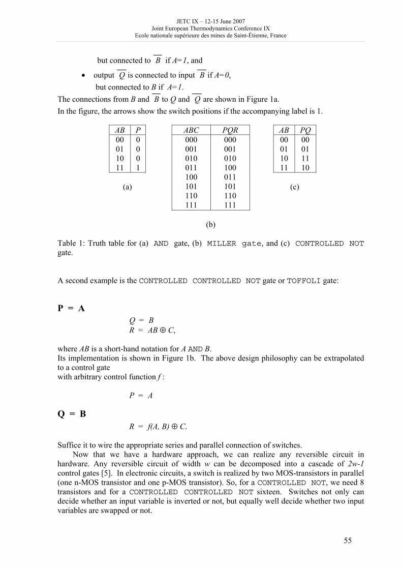
JETC IX – 12-15 June 2007 Joint European Thermodynamics Conference IX
Ecole nationale supérieure des mines de Saint-Étienne, France
55
but connected to B if A=1, and
• output Q is connected to input B if A=0, but connected to B if A=1.
The connections from B and B to Q and Q are shown in Figure 1a. In the figure, the arrows show the switch positions if the accompanying label is 1.
AB P ABC PQR AB PQ 00 01 10 11
0 0 0 1
00 01 10 11
00 01 11 10
(a)
000 001 010 011 100 101 110 111
000 001 010 100 011 101 110 111
(c)
(b)
Table 1: Truth table for (a) AND gate, (b) MILLER gate, and (c) CONTROLLED NOT gate. A second example is the CONTROLLED CONTROLLED NOT gate or TOFFOLI gate:
P = A Q = B R = AB ⊕ C,
where AB is a short-hand notation for A AND B. Its implementation is shown in Figure 1b. The above design philosophy can be extrapolated to a control gate with arbitrary control function f :
P = A
Q = B R = f(A, B) ⊕ C.
Suffice it to wire the appropriate series and parallel connection of switches.
Now that we have a hardware approach, we can realize any reversible circuit in hardware. Any reversible circuit of width w can be decomposed into a cascade of 2w-1 control gates [5]. In electronic circuits, a switch is realized by two MOS-transistors in parallel (one n-MOS transistor and one p-MOS transistor). So, for a CONTROLLED NOT, we need 8 transistors and for a CONTROLLED CONTROLLED NOT sixteen. Switches not only can decide whether an input variable is inverted or not, but equally well decide whether two input variables are swapped or not.
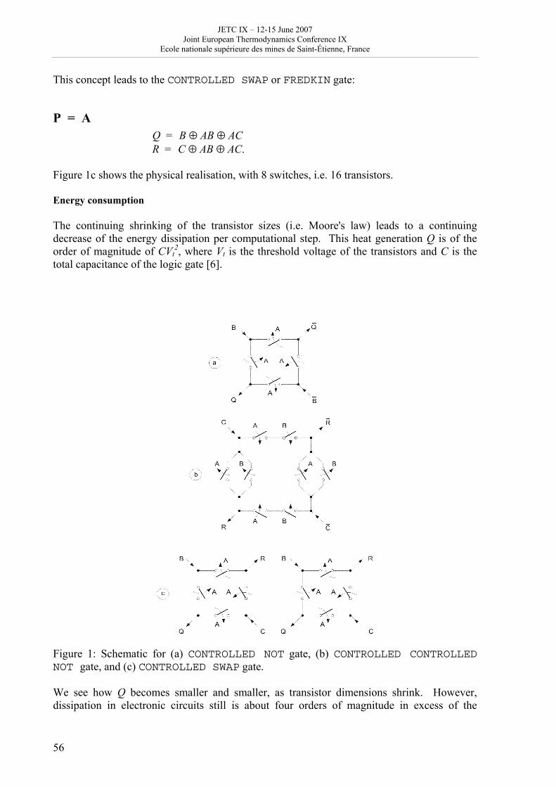
JETC IX – 12-15 June 2007 Joint European Thermodynamics Conference IX
Ecole nationale supérieure des mines de Saint-Étienne, France
56
This concept leads to the CONTROLLED SWAP or FREDKIN gate:
P = A Q = B ⊕ AB ⊕ AC R = C ⊕ AB ⊕ AC.
Figure 1c shows the physical realisation, with 8 switches, i.e. 16 transistors. Energy consumption The continuing shrinking of the transistor sizes (i.e. Moore's law) leads to a continuing decrease of the energy dissipation per computational step. This heat generation Q is of the order of magnitude of CVt
2, where Vt is the threshold voltage of the transistors and C is the total capacitance of the logic gate [6].
Figure 1: Schematic for (a) CONTROLLED NOT gate, (b) CONTROLLED CONTROLLED NOT gate, and (c) CONTROLLED SWAP gate. We see how Q becomes smaller and smaller, as transistor dimensions shrink. However, dissipation in electronic circuits still is about four orders of magnitude in excess of the
JETC IX – 12-15 June 2007 Joint European Thermodynamics Conference IX
Ecole nationale supérieure des mines de Saint-Étienne, France
57
Landauer quantum kT log(2), which amounts (for T = 300K) to about 3 × 10-21 J or 3 zeptojoule.
Further shrinking of transistor width and length and further reduction of Vt ultimately will lead to a Q value in the neighbourhood of kT log(2). That day, digital electronics will have good reason to be reversible, because entropy generation, caused by throwing away bits of information, will then be the main source of heat generation in chips. According to the International Technology Roadmap of Semiconductors [7] we may expect this to happen around 2036. This, however, does not mean that the reversible MOS circuits are useless today. Indeed, as they are a reversible form of pass-transistor topology, they are particularly suited for so-called adiabatic addressing. Here, all signals are gradually set, first to an intermediate level, then to their final values. In practice, such procedure leads to a factor of about 10 in power reduction [6].
References [1] I. Markov (2003). An introduction to reversible circuits. Proceedings of the Int. Workshop on Logic and Synthesis, Laguna Beach, 318-319. [2] A. De Vos (2003). Lossless computing. Proceedings of the IEEE Workshop on Signal Processing, Poznań, 7-14. [3] B. Hayes (2006). Reverse engineering. American Scientist 94 107-111. [4] R. Feynman (1985). Quantum mechanical computers. Optics News 11 11-20. [5] Y. Van Rentergem and A. De Vos (2007). Synthesis and optimization of reversible circuits. Proceedings of the 2007 Reed-Muller Workshop, Oslo. [6] A. De Vos and Y. Van Rentergem (2005). Energy dissipation in reversible logic addressed by a ramp voltage. Proceedings of the 15th Int. PATMOS Workshop, Leuven, 207-216. [7] P. Zeitzoff and J. Chang (Jan/Feb 2005). A perspective from the 2003 ITRS. IEEE Circuits & Devices Magazine 21 4-15.
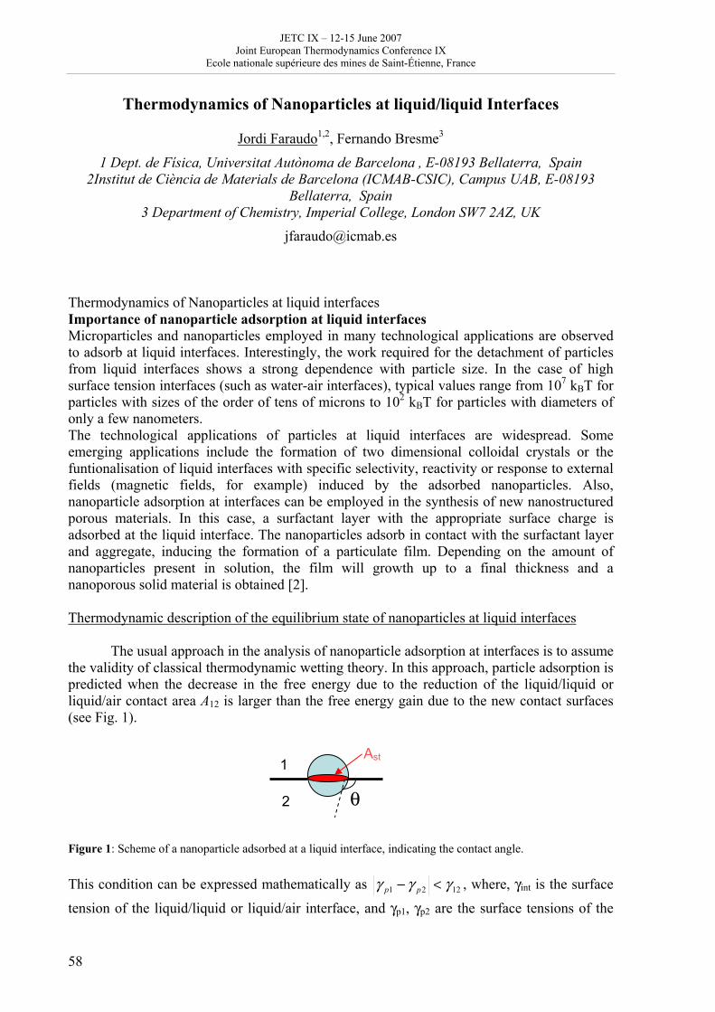
JETC IX – 12-15 June 2007 Joint European Thermodynamics Conference IX
Ecole nationale supérieure des mines de Saint-Étienne, France
58
Thermodynamics of Nanoparticles at liquid/liquid Interfaces
Jordi Faraudo1,2, Fernando Bresme3
1 Dept. de Física, Universitat Autònoma de Barcelona , E-08193 Bellaterra, Spain 2Institut de Ciència de Materials de Barcelona (ICMAB-CSIC), Campus UAB, E-08193
Bellaterra, Spain 3 Department of Chemistry, Imperial College, London SW7 2AZ, UK
[email protected] Thermodynamics of Nanoparticles at liquid interfaces Importance of nanoparticle adsorption at liquid interfaces Microparticles and nanoparticles employed in many technological applications are observed to adsorb at liquid interfaces. Interestingly, the work required for the detachment of particles from liquid interfaces shows a strong dependence with particle size. In the case of high surface tension interfaces (such as water-air interfaces), typical values range from 107 kBT for particles with sizes of the order of tens of microns to 102 kBT for particles with diameters of only a few nanometers. The technological applications of particles at liquid interfaces are widespread. Some emerging applications include the formation of two dimensional colloidal crystals or the funtionalisation of liquid interfaces with specific selectivity, reactivity or response to external fields (magnetic fields, for example) induced by the adsorbed nanoparticles. Also, nanoparticle adsorption at interfaces can be employed in the synthesis of new nanostructured porous materials. In this case, a surfactant layer with the appropriate surface charge is adsorbed at the liquid interface. The nanoparticles adsorb in contact with the surfactant layer and aggregate, inducing the formation of a particulate film. Depending on the amount of nanoparticles present in solution, the film will growth up to a final thickness and a nanoporous solid material is obtained [2]. Thermodynamic description of the equilibrium state of nanoparticles at liquid interfaces The usual approach in the analysis of nanoparticle adsorption at interfaces is to assume the validity of classical thermodynamic wetting theory. In this approach, particle adsorption is predicted when the decrease in the free energy due to the reduction of the liquid/liquid or liquid/air contact area A12 is larger than the free energy gain due to the new contact surfaces (see Fig. 1). Figure 1: Scheme of a nanoparticle adsorbed at a liquid interface, indicating the contact angle. This condition can be expressed mathematically as 1221 γγγ <− pp , where, γint is the surface
tension of the liquid/liquid or liquid/air interface, and γp1, γp2 are the surface tensions of the
θ
1
2
Ast
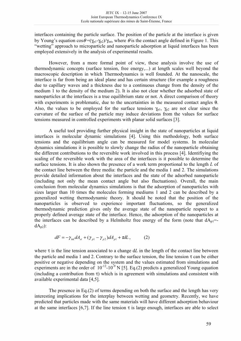
JETC IX – 12-15 June 2007 Joint European Thermodynamics Conference IX
Ecole nationale supérieure des mines de Saint-Étienne, France
59
interfaces containing the particle surface. The position of the particle at the interface is given by Young’s equation cosθ =(γp1-γp2)/γint, where θ is the contact angle defined in Figure 1. This “wetting” approach to microparticle and nanoparticle adsorption at liquid interfaces has been employed extensively in the analysis of experimental results. However, from a more formal point of view, these analysis involve the use of thermodynamic concepts (surface tension, free energy,...) at length scales well beyond the macroscopic description in which Thermodynamics is well founded. At the nanoscale, the interface is far from being an ideal plane and has certain structure (for example a roughness due to capillary waves and a thickness due to a continuous change from the density of the medium 1 to the density of the medium 2). It is also not clear whether the adsorbed state of nanoparticles at the interfaces is a true equilibrium state or not. A direct comparison of theory with experiments is problematic, due to the uncertainties in the measured contact angles θ. Also, the values to be employed for the surface tensions γp1, γp2 are not clear since the curvature of the surface of the particle may induce deviations from the values for surface tensions measured in controlled experiments with planar solid surfaces [3].
A useful tool providing further physical insight in the state of nanoparticles at liquid interfaces is molecular dynamic simulations [4]. Using this methodology, both surface tensions and the equilibrium angle can be measured for model systems. In molecular dynamics simulations it is possible to slowly change the radius of the nanoparticle obtaining the different contributions to the reversible work involved in this process [4]. Identifiying the scaling of the reversible work with the area of the interfaces is it possible to determine the surface tensions. It is also shown the presence of a work term proportional to the length L of the contact line between the three media: the particle and the media 1 and 2. The simulations provide detailed information about the interfaces and the state of the adsorbed nanoparticle (including not only the mean contact angle but also fluctuations). Overall, the main conclusion from molecular dynamics simulations is that the adsorption of nanoparticles with sizes larger than 10 times the molecules forming mediums 1 and 2 can be described by a generalized wetting thermodynamic theory. It should be noted that the position of the nanoparticles is observed to experience important fluctuations, so the generalized thermodynamic prediction gives only the average state of the nanoparticle respect to a properly defined average state of the interface. Hence, the adsorption of the nanoparticles at the interfaces can be described by a Helmholtz free energy of the form (note that dAp1=-dAp2): dLdAdAdF pppst τγγγ +−+−= 121int )( , (2) where τ is the line tension associated to a change dL in the length of the contact line between the particle and media 1 and 2. Contrary to the surface tension, the line tension τ can be either positive or negative depending on the system and the values estimated from simulations and experiments are in the order of 10-12-10-9 N [5]. Eq.(2) predicts a generalized Young equation (including a contribution from τ) which is in agreement with simulations and consistent with available experimental data [4,5]. The presence in Eq.(2) of terms depending on both the surface and the length has very interesting implications for the interplay between wetting and geometry. Recently, we have predicted that particles made with the same materials will have different adsorption behaviour at the same interfaces [6,7]. If the line tension τ is large enough, interfaces are able to select
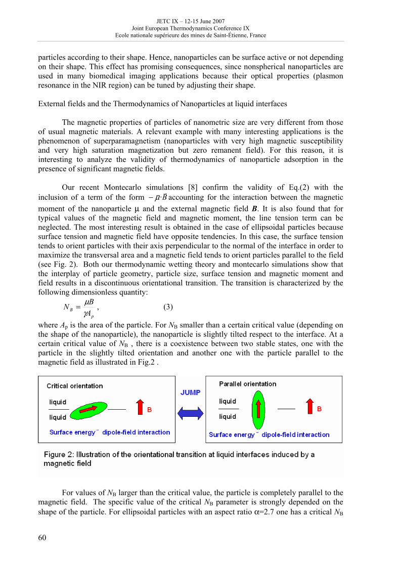
JETC IX – 12-15 June 2007 Joint European Thermodynamics Conference IX
Ecole nationale supérieure des mines de Saint-Étienne, France
60
particles according to their shape. Hence, nanoparticles can be surface active or not depending on their shape. This effect has promising consequences, since nonspherical nanoparticles are used in many biomedical imaging applications because their optical properties (plasmon resonance in the NIR region) can be tuned by adjusting their shape. External fields and the Thermodynamics of Nanoparticles at liquid interfaces
The magnetic properties of particles of nanometric size are very different from those of usual magnetic materials. A relevant example with many interesting applications is the phenomenon of superparamagnetism (nanoparticles with very high magnetic susceptibility and very high saturation magnetization but zero remanent field). For this reason, it is interesting to analyze the validity of thermodynamics of nanoparticle adsorption in the presence of significant magnetic fields.
Our recent Montecarlo simulations [8] confirm the validity of Eq.(2) with the
inclusion of a term of the form Brr·μ− accounting for the interaction between the magnetic
moment of the nanoparticle μ and the external magnetic field B. It is also found that for typical values of the magnetic field and magnetic moment, the line tension term can be neglected. The most interesting result is obtained in the case of ellipsoidal particles because surface tension and magnetic field have opposite tendencies. In this case, the surface tension tends to orient particles with their axis perpendicular to the normal of the interface in order to maximize the transversal area and a magnetic field tends to orient particles parallel to the field (see Fig. 2). Both our thermodynamic wetting theory and montecarlo simulations show that the interplay of particle geometry, particle size, surface tension and magnetic moment and field results in a discontinuous orientational transition. The transition is characterized by the following dimensionless quantity:
pB A
BNγμ= , (3)
where Ap is the area of the particle. For NB smaller than a certain critical value (depending on the shape of the nanoparticle), the nanoparticle is slightly tilted respect to the interface. At a certain critical value of NB , there is a coexistence between two stable states, one with the particle in the slightly tilted orientation and another one with the particle parallel to the magnetic field as illustrated in Fig.2 .
For values of NB larger than the critical value, the particle is completely parallel to the magnetic field. The specific value of the critical NB parameter is strongly depended on the shape of the particle. For ellipsoidal particles with an aspect ratio α=2.7 one has a critical NB
JETC IX – 12-15 June 2007 Joint European Thermodynamics Conference IX
Ecole nationale supérieure des mines de Saint-Étienne, France
61
about 0.15. The more favourable conditions to observe these transitions predicted in this work correspond to superparamagnetic nanoparticles with intermediate anisotropies (major/minor axes ≈3/2–2) at surfaces with low interfacial tensions. For example, for a typical superparamagnetic particle (magnetic susceptibility χ ≈ 10) with a major axis about 3000 nm and 1.6 anisotropy at an interface with a surface tension about 10 mN/m we obtain the orientational transition (NB = 0.15) using a magnetic field of about 0.02 T. In the case of stronger magnetic fields (about 0.1 T), typical superparamagnetic particles have a saturation magnetic moment of about μ ≈ 80 A m2 kg−1, so orientational transitions can in principle be observed at a water/air interface (γ ≈ 73 mN m−1).
References
[1] Pieranski P 1980 Phys. Rev. Lett. 45 569. [2] Fendler J.H. and Meldrum F.C. 1995 Adv. Mat. 7 607. [3] J. S. Rowlinson and B. Widom, Molecular Theory of Capillarity, Oxford University Press, Belfast, 1989. [4] Bresme F and Quirke N 1998 Phys. Rev. Lett. 80 3791 [5] Aveyard, R., Clint, J.H., Particle wettability and line tension, J. Chem. Soc. Faraday Trans., 92 (1996), 85–89. [6] Faraudo J and Bresme F 2003 J. Chem. Phys. 118 6518 [7] Faraudo J and Bresme F 2004 J. Non-Equilib. Thermodyn. 29 397 [8] Bresme F and Faraudo J 2007 J. Phys Condensed Matter (accepted for publication)
JETC IX – 12-15 June 2007 Joint European Thermodynamics Conference IX
Ecole nationale supérieure des mines de Saint-Étienne, France
62
What’s new with thermodynamical optimisation of refrigerating machines, with regards to design and control-command: a review synthesis
M. Feidt 1, M. Karkri 1, R. Boussehain 1, M. Costea2, C. Petre2, S. Petrescu2 1 LEMTA-UHP, NANCY, France
2 Faculté de Génie Mécanique, UPB BUCAREST, Roumanie
[email protected] Abstract A research program has been recently initiated by CEMAGREF (France). This project intend to have a better knowledge of how to design, control and command industrial refrigerating machines, mainly mechanical vapor compression configurations. In the beginning of the program, it appears useful to do a review of the state of the art and particularly the most recent thermodynamical developpements, part of which is denominated Finite Time Thermodynamics. The corresponding approach is a lumped one (macroscopic thermodynamical model). It intend to characterize with a minimum of site data the functional evolution of the design with respect to use (optimal rise of a system for various applications and not only for maximum or nominal use). The goal is to suggest robust and relevant models on the basis of the few experimental data. The question is, whether we should measures some other data, to dispose of more information and what is the expected gain (at least in control command). After twenty years of consideration [1], we suggest here a review in terms of : Applications [24], concepts [24,7,30] and analysis methodology [31,32 ,33]. 1. Introduction Finite time study of energy systems has been rediscovered with the publication of CURZON and AHLBORN, through the nice radical formulation:
( ) SCSF TTMaxW /1−=η (1) This relation gives the efficiency of a thermomechanical engine in contact with two thermostats (hot side SCT , cold side SFT ) at maximum [1]. This was previously done in 1957 inside publications of CHAMBADAL and NOVIKOV. Since then numerous works have been published for a great variety of engines criteria and constraints [2,3]. The same approach has been recently suggested for inverse cycle machines. The first two papers are from Blanchard (1980) and Y. Goth and M Feidt [4]. Since than numerous papers have been published in many laboratory and in our research group. We specify here tow review papers recently published in books [26 27]. One of the last published paper is relative to ferromagnetic sterling refrigerator in contact with two finite thermal capacities [10]. We intend to show here that the precedent theoretical works could be helpful in order to optimize inverse cycle machines. Two main goals appear for this purpose : (i) Optimum design of a machine to fulfil an identified demand (design optimisation or static optimisation); (ii) Optimum command of a given machine, to adapt the system at the demand evolution with time (control optimisation, or dynamic optimisation). 2. Review of existing models 2. 1. GORDON’s works For 10 years, GORDON studied the inverse cycle machine in order to prove the usefulness of
F.T.T to check in situ performance of the machines with a minimum of measurement information. And to propose robust but physical model control-command of the machine.
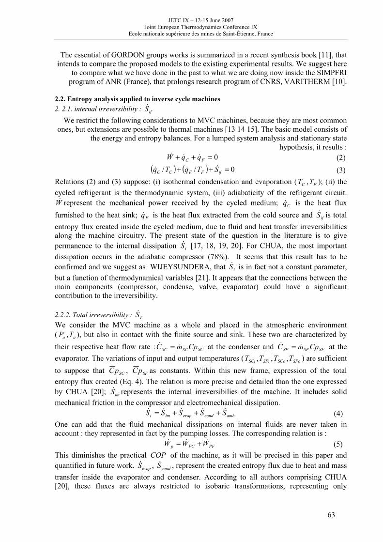
JETC IX – 12-15 June 2007 Joint European Thermodynamics Conference IX
Ecole nationale supérieure des mines de Saint-Étienne, France
63
The essential of GORDON groups works is summarized in a recent synthesis book [11], that intends to compare the proposed models to the existing experimental results. We suggest here
to compare what we have done in the past to what we are doing now inside the SIMPFRI program of ANR (France), that prolongs research program of CNRS, VARITHERM [10].
2.2. Entropy analysis applied to inverse cycle machines 2. 2.1. internal irreversibility : ifS&
We restrict the following considerations to MVC machines, because they are most common ones, but extensions are possible to thermal machines [13 14 15]. The basic model consists of
the energy and entropy balances. For a lumped system analysis and stationary state hypothesis, it results :
0=++ FC qqW &&& (2)( ) ( ) 0// =++ ifFFCC STqTq &&& (3)
Relations (2) and (3) suppose: (i) isothermal condensation and evaporation ( CT , FT ); (ii) the cycled refrigerant is the thermodynamic system, (iii) adiabaticity of the refrigerant circuit. W& represent the mechanical power received by the cycled medium; Cq& is the heat flux furnished to the heat sink; Fq& is the heat flux extracted from the cold source and ifS& is total entropy flux created inside the cycled medium, due to fluid and heat transfer irreversibilities along the machine circuitry. The present state of the question in the literature is to give permanence to the internal dissipation iS& [17, 18, 19, 20]. For CHUA, the most important dissipation occurs in the adiabatic compressor (78%). It seems that this result has to be confirmed and we suggest as WIJEYSUNDERA, that iS& is in fact not a constant parameter, but a function of thermodynamical variables [21]. It appears that the connections between the main components (compressor, condense, valve, evaporator) could have a significant contribution to the irreversibility. 2.2.2. Total irreversibility : TS& We consider the MVC machine as a whole and placed in the atmospheric environment ( aP , aT ), but also in contact with the finite source and sink. These two are characterized by their respective heat flow rate : SCSCSC CpmC && = at the condenser and SFSFSF CpmC && = at the evaporator. The variations of input and output temperatures ( SFiSCi TT , , SFoSCo TT , ) are sufficient to suppose that SCpC , SFpC as constants. Within this new frame, expression of the total entropy flux created (Eq. 4). The relation is more precise and detailed than the one expressed by CHUA [20]; imS& represents the internal irreversibilies of the machine. It includes solid mechanical friction in the compressor and electromechanical dissipation.
ambcondevapimt SSSSS &&&&& +++= (4) One can add that the fluid mechanical dissipations on internal fluids are never taken in account : they represented in fact by the pumping losses. The corresponding relation is :
PFPCp WWW &&& += (5) This diminishes the practical COP of the machine, as it will be precised in this paper and quantified in future work. evapS& , condS& , represent the created entropy flux due to heat and mass transfer inside the evaporator and condenser. According to all authors comprising CHUA [20], these fluxes are always restricted to isobaric transformations, representing only
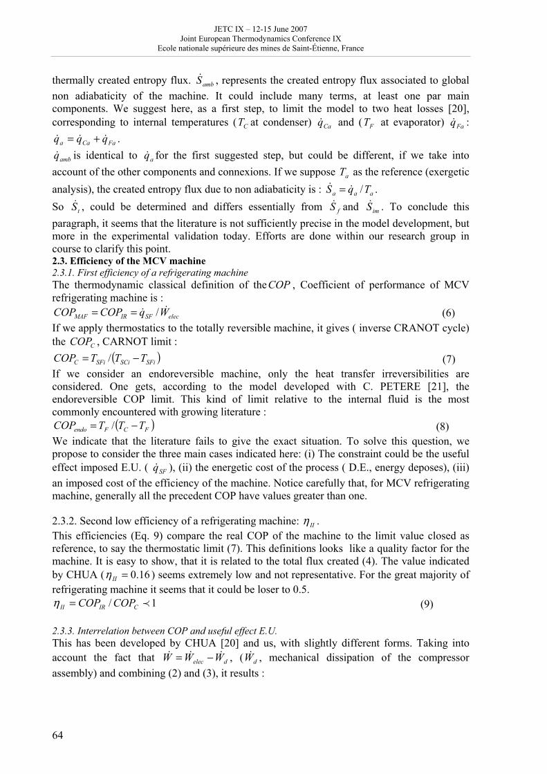
JETC IX – 12-15 June 2007 Joint European Thermodynamics Conference IX
Ecole nationale supérieure des mines de Saint-Étienne, France
64
thermally created entropy flux. ambS& , represents the created entropy flux associated to global non adiabaticity of the machine. It could include many terms, at least one par main components. We suggest here, as a first step, to limit the model to two heat losses [20], corresponding to internal temperatures ( CT at condenser) Caq& and ( FT at evaporator) Faq& :
FaCaa qqq &&& += .
ambq& is identical to aq& for the first suggested step, but could be different, if we take into account of the other components and connexions. If we suppose aT as the reference (exergetic analysis), the created entropy flux due to non adiabaticity is : aaa TqS /&& = . So tS& , could be determined and differs essentially from fS& and imS& . To conclude this paragraph, it seems that the literature is not sufficiently precise in the model development, but more in the experimental validation today. Efforts are done within our research group in course to clarify this point. 2.3. Efficiency of the MCV machine 2.3.1. First efficiency of a refrigerating machine The thermodynamic classical definition of theCOP , Coefficient of performance of MCV refrigerating machine is :
elecSFIRMAF WqCOPCOP && /== (6) If we apply thermostatics to the totally reversible machine, it gives ( inverse CRANOT cycle) the CCOP , CARNOT limit :
( )SFiSCiSFiC TTTCOP −= / (7) If we consider an endoreversible machine, only the heat transfer irreversibilities are considered. One gets, according to the model developed with C. PETERE [21], the endoreversible COP limit. This kind of limit relative to the internal fluid is the most commonly encountered with growing literature :
( )FCFendo TTTCOP −= / (8) We indicate that the literature fails to give the exact situation. To solve this question, we propose to consider the three main cases indicated here: (i) The constraint could be the useful effect imposed E.U. ( SFq& ), (ii) the energetic cost of the process ( D.E., energy deposes), (iii) an imposed cost of the efficiency of the machine. Notice carefully that, for MCV refrigerating machine, generally all the precedent COP have values greater than one. 2.3.2. Second low efficiency of a refrigerating machine: IIη . This efficiencies (Eq. 9) compare the real COP of the machine to the limit value closed as reference, to say the thermostatic limit (7). This definitions looks like a quality factor for the machine. It is easy to show, that it is related to the total flux created (4). The value indicated by CHUA ( 16.0=IIη ) seems extremely low and not representative. For the great majority of refrigerating machine it seems that it could be loser to 0.5.
1/ pCIRII COPCOP=η (9) 2.3.3. Interrelation between COP and useful effect E.U. This has been developed by CHUA [20] and us, with slightly different forms. Taking into account the fact that delec WWW &&& −= , ( dW& , mechanical dissipation of the compressor assembly) and combining (2) and (3), it results :
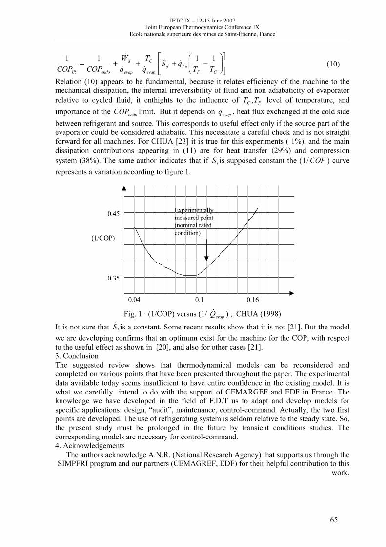
JETC IX – 12-15 June 2007 Joint European Thermodynamics Conference IX
Ecole nationale supérieure des mines de Saint-Étienne, France
65
⎥⎦
⎤⎢⎣
⎡⎟⎟⎠
⎞⎜⎜⎝
⎛−+++=
CFFaif
evap
C
evap
d
endoIR TTqS
qT
qW
COPCOP1111
&&&&
& (10)
Relation (10) appears to be fundamental, because it relates efficiency of the machine to the mechanical dissipation, the internal irreversibility of fluid and non adiabaticity of evaporator relative to cycled fluid, it enthights to the influence of FC TT , level of temperature, and importance of the endoCOP limit. But it depends on evapq& , heat flux exchanged at the cold side between refrigerant and source. This corresponds to useful effect only if the source part of the evaporator could be considered adiabatic. This necessitate a careful check and is not straight forward for all machines. For CHUA [23] it is true for this experiments ( 1%), and the main dissipation contributions appearing in (11) are for heat transfer (29%) and compression system (38%). The same author indicates that if iS& is supposed constant the ( COP/1 ) curve represents a variation according to figure 1.
(1/COP)
Experimentally measured point (nominal rated condition)
0.04 0.1 0.16
0.35
0.45
Fig. 1 : (1/COP) versus (1/ evapQ& ) , CHUA (1998)
It is not sure that iS& is a constant. Some recent results show that it is not [21]. But the model we are developing confirms that an optimum exist for the machine for the COP, with respect to the useful effect as shown in [20], and also for other cases [21]. 3. Conclusion The suggested review shows that thermodynamical models can be reconsidered and completed on various points that have been presented throughout the paper. The experimental data available today seems insufficient to have entire confidence in the existing model. It is what we carefully intend to do with the support of CEMARGEF and EDF in France. The knowledge we have developed in the field of F.D.T us to adapt and develop models for specific applications: design, “audit”, maintenance, control-command. Actually, the two first points are developed. The use of refrigerating system is seldom relative to the steady state. So, the present study must be prolonged in the future by transient conditions studies. The corresponding models are necessary for control-command. 4. Acknowledgements
The authors acknowledge A.N.R. (National Research Agency) that supports us through the SIMPFRI program and our partners (CEMAGREF, EDF) for their helpful contribution to this
work.
JETC IX – 12-15 June 2007 Joint European Thermodynamics Conference IX
Ecole nationale supérieure des mines de Saint-Étienne, France
66
References : [1] M.FEIDT, Thermodynamique et optimisation énergétique de système et Procédés, TEC et DOC, 2ième édition, 1996, 3ième partie, p339-379. [2] M.FEIDT, Energétique, concepts et applications, Dunod, Oct. 2006, (chapitre, 18-19). [3] S.M. GORDON, M. HULEILIL, General performance characteristics of real heat engines, J. of Appl. Phy. Aug. 1992, 72 (3), p 829-837. [4] Y.GOTH, M. FEIDT, Recherche des conditions optimales de fonctionnement des pompes à chaleur au machine à froid associés à un cycle de CARNOT endoreversible, C,R. Acad. Sci., Paris, série II, p113-122. [5] M. FEIDT, Thermodynamique et optimisation énergétique de systèmes et procédés, TEC et DOC, 2ième édition, 1996, 3ième partie (chapitre 4), p381-403. [6] M.FEIDT, Energétique, concepte et applications, Dumod, Oct. 2006, chapitre 15. [7] M.FEIDT, Production de Froid et revalorisation de la chaleur: principes généraux, T.I, BE8095 (10.1998). [8] M.FEIDT, Production de Froid et revalorisation de la chaleur: machines particulières, T.I. BE8096 (10.2003). [9] M.FEIDT,Production de Froid et revalorisation de la chaleur: machines cryogéniques, T. I.BE8097 (10.2005). [10] Y. XINGMFI et al., Performance optimisation of an irreversible ferromagnetic Stirling refrigerator with finite thermal sources, Proc, of ECOS, 2006, Greet, Greece, July 12-14,2006, p 1303-1318. [11] J.M. GORDON et al., Cool Thermodynamics, Cambridge Int. Sciences Publishers (2000). [12] P.SCHALBAERT, Modélisation du comportement des systèmes thermiques: application aux groupes frigorifiques, DEA, INA Lyon, Juillet 2003. [13] L. GROSU, M. FEIDT, R. BÉNELMIR, Study of the improvement in the performance coefficient of machines operating with three heat reservoirs, Int. J. Exergy, 1 (1) (2004), 147-162. [14] E. VASILESCU, M. FEIDT, R. BOUSSEHAIN, L'optimisation des cycles idéaux exo-irréversibles des systèmes frigorifiques quadrithermes, Proceedings COFRET'04, 22-24 Avril 2004, Nancy, France. [15] M.FEIDT, Tentative unified description of engines refrigerators and heat pomp in contact with two or three heat reservoirs, chapter 26, in Recent advances in FTT, editor c.w.u et al., Nova science Pal. 1999, p 449-471. [16] M. FEIDT, comportement en régime variable ou hors nominal de machines thermiques à cycles inverse et de leurs composants, rapport Varitherm, 2005. [17] J.M. GORDON, NG K.C., thermodynamic modelling of reciprocating chillers, I. J. of Apll. Phy. 75, 1994, p 2769-2774. [18] J.M. GORDON, NG K.C., Predictive and diagnostic aspects of universal thermodynamic model for chillers, Int. J.H.M.T, 38, 1995, p 807-815. [19] J.M. GORDON et al., centrifugal chillers: thermodynamic modelling and a diagnostic case study, I. J. of Ref, vol. 18, n° 4, 1995, p 253-257. [20] M.T. CHUA et al., Experimental study of the fundamental properties of reciprocating chillers and their relation to thermodynamic modelling and chiller design, Int. J.H.M.T, 39, 1996, p2195-2204. [21] C. PETRE et al., modélisation et optimisation d’une pompe à chaleur avec des contraintes, SFT, 2006.
JETC IX – 12-15 June 2007 Joint European Thermodynamics Conference IX
Ecole nationale supérieure des mines de Saint-Étienne, France
67
[22] NG K.C. et al., The role of internal dissipation and process average temperature in chillers performance and diagnostics, J. of Appl. Phy., vol. 83, n° 4, 1998, p 1831-1836. [23] H.T. CHUA, Universal thermodynamic modelling of chillers: special application to adsorption chillers, PHD, national university Singapour (272 p), 1998. [24] NG. KC et al., Diagnostic and optimization of reciprocating chillers: theory and experiments, Apll. Therm. Eng., vol. 17, n° 3, 1997, p 263-276. [25] G. BRAZZINI, Irreversible refrigerators with isothermal heat exchanges, Rev., Int. Froid, n°2, 1993, p101-106. [26] M. FIEDT, Thermodynamics and optimisation of reverses cycle machines refrigeration, heat pump, air conditioning, cryogenics in thermodynamic optimization of complex systems, Kluver. Acad, 1999, p 403-410. [27] M. FEIDT, Advanced thermodynamics of reverse cycle machine, in low temperature and cryogenic Ref. Kluver Acad., 2003, p 39-82. [28] J. PHELAN et al., In situ performance testing of chillers for Energy Analysis, ASHRE Trans., vol 103, n°1, 1997, p 290.302. [29] J.M.GORDON, K.C. NG, Cool thermodynamics, Cambridge int. science publishing, 2000. [30]M. FEIDT, Thermodynamics and optimization of reverse cycle machines : refrigeration heat pump, air conditioning, cryogenics, Thermodynamic optimisation of complex energy systems, Kluwer Academic, p 385-401, 1999. [31] M. FEIDT, Recent advances in Finite Time Thermodynamics", chap. 26, p 449-471, Editors C. WU, L. CHEN, J. CHEN, Nova science publishers, 1999. [32] M. FEIDT , Depletion of ozone and greenhouse effect, a new goal for the design of inverse cycle machines" Int. J. Energy research, special issue edited by A. Bejan et al, vol. 26 n° 7, p 653-674, 2002. [33] M. FEIDT, Advanced Thermodynamics of reverse cycle machine" in S. KAKAC et al, eds, Low temperature and cryogenic refrigeration, Kluwer Academic Press, p 39-82, 2003.
JETC IX – 12-15 June 2007 Joint European Thermodynamics Conference IX
Ecole nationale supérieure des mines de Saint-Étienne, France
68
Quantum surface energy and lateral forces in ideal gases
Coskun Firat and Altug Sisman*
Istanbul Technical University, Energy Institute, 34469 Maslak, Istanbul, Turkey.
[email protected], [email protected] Abstract: Gas particles confined in a finite domain non-locally interact with the boundaries due to their wave character. This non-local interaction causes a non-homogeneous density distribution even for an ideal gas at thermodynamic equilibrium. Non-homogeneity of gas density gives rise to a surface energy. Since it is originated from the wave character of the particles, it is called quantum surface energy (QSE). As a result of QSE, a quantum surface tension appears and becomes important for the systems in nano-scale while it is negligible for macro systems. Because of QSE, thermodynamic state functions of even an ideal gas not only depend on two intensive parameters, like temperature and density, but also on size and shape of the domain. Therefore, additivity of extensive quantities is not valid anymore and size and shape become additional control parameters on thermodynamic state. In this study, QSE of an ideal gas confined in a domain of an arbitrary shape is derived. For rectangular, cylindrical and spherical domains, local gas density distributions are also analytically determined. It is seen that there is a layer near to the boundaries of the domain and the gas density goes to zero within this layer due to non-local interactions of the particles with the boundaries. This layer is called quantum boundary layer (QBL) since its thickness goes to zero when ∇ goes to zero. It seems that quantum surface energy is a consequence of QBL. A movable wall which separates a rectangular box filled by an ideal gas into two parts is subjected to a repulsive lateral force due to quantum boundary layer. This non-classical effect may experimentally be verified as a macroscopic manifestation of QSE. 1. Introduction
In recent years, a great progress has been made in producing macro/nanostructures which provokes the design of micro/nano engines like gas turbines, heat exchangers and combustors [1-3]. It is known that the thermodynamics become different in micro/nano scale due to both classical and quantum size effects. Thermodynamic state functions of a gas confined in such a small scale depend also on shape and size of the domain besides two usual intensive variables, like temperature and density. These additional control variables may lead to design some new devices.
Dependence of global thermodynamic properties on shape and size of the confinement domain has been studied for classical and quantum ideal gases [4-14]. Shape and size dependencies of the global properties of ideal gases originate from quantum surface energy (QSE) [4, 9]. Analytical expressions for QSE have been given for rectangular, cylindrical and spherical geometries in literature [9].
Recently, it has been shown that the local density distribution of an ideal gas confined in a rectangular domain is not homogenous even at equilibrium state and there is a boundary layer in which the density goes to zero [4]. This layer has been called quantum boundary layer (QBL) since its thickness goes to zero when ∇ 0. QBL gives a basic and clear explanation for the origin of QSE in a rectangular domain.
JETC IX – 12-15 June 2007 Joint European Thermodynamics Conference IX
Ecole nationale supérieure des mines de Saint-Étienne, France
69
In this study, a Maxwellian ideal gas is considered and a generalized expression of QSE for a confinement domain of an arbitrary shape is obtained. For cylindrical and spherical confinement domains, density distributions are derived and examined. For the thickness of QBL, a general and simple analytical expression is obtained. It is shown that a movable wall of zero thickness which separates a rectangular box filled by an ideal gas into two parts is subjected to a repulsive force due to QBL. 2. Quantum surface energy of an ideal gas in a finite domain of an arbitrary shape All thermodynamic properties of a system can be calculated when the partition function is known. The partition function consists of a summation over the energy eigenvalues of the stationary Schrödinger equation. For macro systems, it is a very good approximation to replace the summation by integration to calculate the partition function. For micro/nano systems, however, it is necessary to use a more precise formula (such as Poisson, Euler-Maclaurin or Abel-Plana formula). The precise calculation of the partition function is the key work in determining the quantum size effects on thermodynamic properties of small systems.
A complete analytical solution of the stationary Schrödinger equation is possible only for a rectangular domain. Even for spherical and cylindrical domains, some approximations should be made to obtain an analytical expression for the energy eigenvalues [9]. For a domain of an arbitrary shape, it is impossible to solve the Schrödinger equation and find the eigenvalues. Fortunately, Weyl’s conjecture gives a precise formula for an asymptotic behavior of the eigenvalue spectrum of the stationary Schrödinger equation [14]. Therefore, it is possible to determine the density of states of eigenvalue spectrum in an asymptotic form for a domain of an arbitrary shape. Consequently, the influence of the confinement geometry on the global thermodynamic properties of an ideal gas can be generalized by using the Weyl’s conjecture.
Stationary Schrödinger equation for a particle confined in a domain bounded by an infinite potential is
022 =+∇ ψκψ in D, 0=∂Dψ (1) where D is a bounded domain of an arbitrary shape and κ is the wave number. According to the Weyl’s conjecture, the number of eigenvalues ( )κNE less than a given eigenvalue κ is given as follows for the asymptotic case ( ∞→κ )
( ) ( ),166
2232 κκ
πκ
πκ oAVNE +−= (2)
where V and A are volume and surface area of the bounded domain D. The second term in Eq.(2) comes from the more precise enumeration of the eigenvalues and it is negligible for macro systems since the surface over volume ratio is too small. On the other hand, it becomes important for micro/nano systems and it is the term where the quantum size effects originate. Therefore, the number of eigenvalues having the value of κ is determined by
( ) ( ) .82
22 κκ
πκκ
πκ
κκκ dAdVd
ddNEg −=≅ (3)
Energy is related with κ by ( ) m222κκε h= , each κ value corresponds a different energy state and ( )κg represents the degeneracy number of an energy state. Single particle partition function and the free energy of an ideal monatomic Maxwellian gas are given by the following expressions respectively
( ) ( )∑ −=κ
κεκζ Tkbeg . (4)
⎥⎦
⎤⎢⎣
⎡+⎟
⎠⎞
⎜⎝⎛−= 1ln
NTNkF b
ζ (5)
JETC IX – 12-15 June 2007 Joint European Thermodynamics Conference IX
Ecole nationale supérieure des mines de Saint-Étienne, France
70
where kb is the Boltzmann’s constant, T is the temperature and N is the total number of particles. By substituting Eq.(3) in Eq.(4) and by use of integral calculation, the partition function is obtained as
⎥⎦
⎤⎢⎣
⎡−=
VAL
LV c
c ππζ
21
8 3
23 (6)
where Lc is the half of the mean de Broglie wavelength defined as TmkhL bc 22= . Thus, free energy is determined as
ππ
21
8ln 3
23cb
cb
ALV
TNknL
TNkF +⎥⎥⎦
⎤
⎢⎢⎣
⎡⎟⎟⎠
⎞⎜⎜⎝
⎛+−= . (7)
The second term in Eq.(7) represents the general form of QSE of an ideal gas confined in a domain of an arbitrary shape. 3. Quantum boundary layer in rectangular, cylindrical and spherical domains
For an ideal Maxwellian gas, the number of particles of quantum state r in a differential local volume dV centered at position xr is expressed as follows [4]
( )[ ]dVxe
eNdN r
r
Tk
Tk
rbr
br 2rψε
ε
⎥⎥⎥⎥
⎦
⎤
⎢⎢⎢⎢
⎣
⎡
=∑ −
− (8)
where N is the total number of particles in the whole confinement volume, rε is the energy eigenvalue of particles corresponding to quantum state r, rψ is the eigenfunction corresponding to quantum state r. In Eq.(8), the term in the first bracket represents the thermodynamic probability to find a particle in quantum state r and the term in the second bracket represents the quantum mechanical probability to find a particle in a volume dV centered at position xr . Hence, the local number density is determined by [4]
( )( )
∑ ∑∑
−
−
==r
r
Tk
rr
Tk
rbr
br
e
xeNnxn ε
ε ψ 2r
r . (9)
Rectangular domain:
For an ideal monatomic gas confined in a rectangular domain, the eigenvalues and eigenfunctions of a particle are well known and the local density given by Eq.(9) has been analytically calculated in Ref. [4] as
( ) ( ) ( ) ( )
⎟⎟⎠
⎞⎜⎜⎝
⎛−⎟⎟
⎠
⎞⎜⎜⎝
⎛−⎟⎟
⎠
⎞⎜⎜⎝
⎛−
=
πα
πα
πα z
z
y
y
x
xcl
zfyfxfnzyxn1
~
1
~
1
~~,~,~ (10)
where ,~xLxx = ,
~yLyy = zLzz =~ , xcx LL=α , ycy LL=α , zcz LL=α and ( )xnx
~ , is given by
( ) ( ) ( )( )⎥⎦⎤
⎢⎣⎡ −⎥⎦⎤
⎢⎣⎡ −= −−− 22 ~1~
11~ xx xxx eexf απαπ . (11)
( )yf y~ and ( )zf z
~ are given by Eq.(11) with αy and αz respectively instead of αx. The dimensionless form of Eq.(10) is written as
( ) ( ) ( ) ( ) ( ).~~~~~~~,~,~~,~,~~ znynxnn
zyxnzyxn zyxcl
== (12)
In figure 1, the variation of ( )xnx~~ versus to xLxx =~ is given. It is seen that the density
distribution is not homogenous and there is a boundary layer in which the density goes to zero. To obtain an analytical expression for the thickness of this layer, density distribution is approximated by a step function (dashed lines in figure 1).
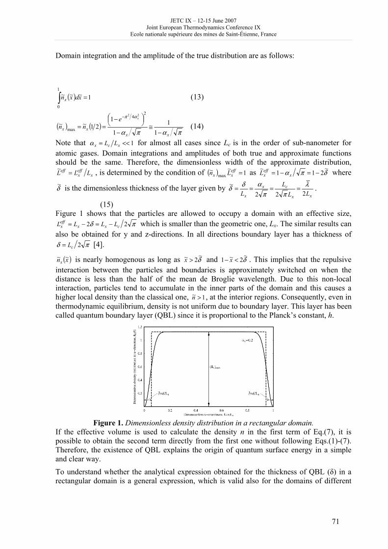
JETC IX – 12-15 June 2007 Joint European Thermodynamics Conference IX
Ecole nationale supérieure des mines de Saint-Étienne, France
71
Domain integration and the amplitude of the true distribution are as follows:
( )∫ =1
0
1~~~ xdxnx (13)
( ) ( )παπα
απ
xxxx
xenn
−≅
−
⎟⎠⎞⎜
⎝⎛ −
==−
11
1
121~~
24
max
22
(14)
Note that 1<<= xcx LLα for almost all cases since Lc is in the order of sub-nanometer for atomic gases. Domain integrations and amplitudes of both true and approximate functions should be the same. Therefore, the dimensionless width of the approximate distribution,
xeffx
eff LLL =~ , is determined by the condition of ( ) 1~~max =eff
xx Ln as δπα ~211~ −=−= xeffxL where
δ~ is the dimensionless thickness of the layer given by xx
cx
x LLL
L 222~ λ
ππαδδ ==== .
(15) Figure 1 shows that the particles are allowed to occupy a domain with an effective size,
πδ 22 cxxeffx LLLL −=−= which is smaller than the geometric one, Lx. The similar results can
also be obtained for y and z-directions. In all directions boundary layer has a thickness of πδ 2cL= [4].
( )xnx~~ is nearly homogenous as long as δ~2~ >x and δ~2~1 <− x . This implies that the repulsive
interaction between the particles and boundaries is approximately switched on when the distance is less than the half of the mean de Broglie wavelength. Due to this non-local interaction, particles tend to accumulate in the inner parts of the domain and this causes a higher local density than the classical one, 1~ >n , at the interior regions. Consequently, even in thermodynamic equilibrium, density is not uniform due to boundary layer. This layer has been called quantum boundary layer (QBL) since it is proportional to the Planck’s constant, h.
Figure 1. Dimensionless density distribution in a rectangular domain.
If the effective volume is used to calculate the density n in the first term of Eq.(7), it is possible to obtain the second term directly from the first one without following Eqs.(1)-(7). Therefore, the existence of QBL explains the origin of quantum surface energy in a simple and clear way.
To understand whether the analytical expression obtained for the thickness of QBL (δ) in a rectangular domain is a general expression, which is valid also for the domains of different
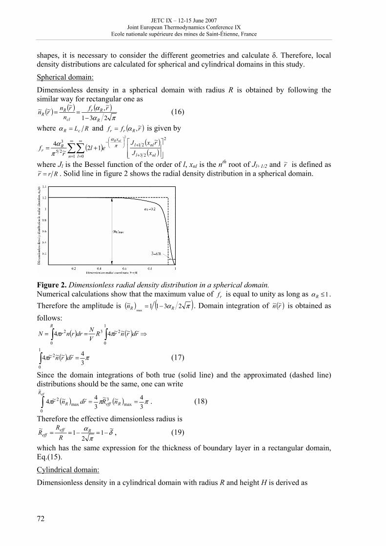
JETC IX – 12-15 June 2007 Joint European Thermodynamics Conference IX
Ecole nationale supérieure des mines de Saint-Étienne, France
72
shapes, it is necessary to consider the different geometries and calculate δ. Therefore, local density distributions are calculated for spherical and cylindrical domains in this study.
Spherical domain:
Dimensionless density in a spherical domain with radius R is obtained by following the similar way for rectangular one as
( ) ( ) ( )πα
α231
~, ~~~
R
Rr
cl
RR
rfn
rnrn−
== (16)
where RLcR =α and ( )rff Rrr~,α= is given by
( ) ( )( )∑∑
∞
=
∞
= +
+⎟⎠⎞
⎜⎝⎛−
⎥⎥⎦
⎤
⎢⎢⎣
⎡+=
1 0
2
23
2125
3 ~12~
42
n l nll
nllx
Rr xJ
rxJel
rf
nlR
πα
πα
where Jl is the Bessel function of the order of l, xnl is the nth root of Jl+1/2 and r~ is defined as Rrr =~ . Solid line in figure 2 shows the radial density distribution in a spherical domain.
Figure 2. Dimensionless radial density distribution in a spherical domain. Numerical calculations show that the maximum value of rf is equal to unity as long as 1≤Rα . Therefore the amplitude is ( ) ( )πα 2311~
max RRn −= . Domain integration of ( )rn ~~ is obtained as follows:
( ) ( )∫∫ ⇒==1
0
23
0
2 ~~~~44 rdrnrRVNdrrnrN
R
ππ
( )∫ =1
0
2
34~~~~4 ππ rdrnr (17)
Since the domain integrations of both true (solid line) and the approximated (dashed line) distributions should be the same, one can write
( ) ( ) πππ34~~
34~~~4
~
0max
3max
2 ==∫effR
ReffR nRrdnr . (18)
Therefore the effective dimensionless radius is
δπ
α ~12
1~ −=−== Reffeff R
RR , (19)
which has the same expression for the thickness of boundary layer in a rectangular domain, Eq.(15).
Cylindrical domain:
Dimensionless density in a cylindrical domain with radius R and height H is derived as
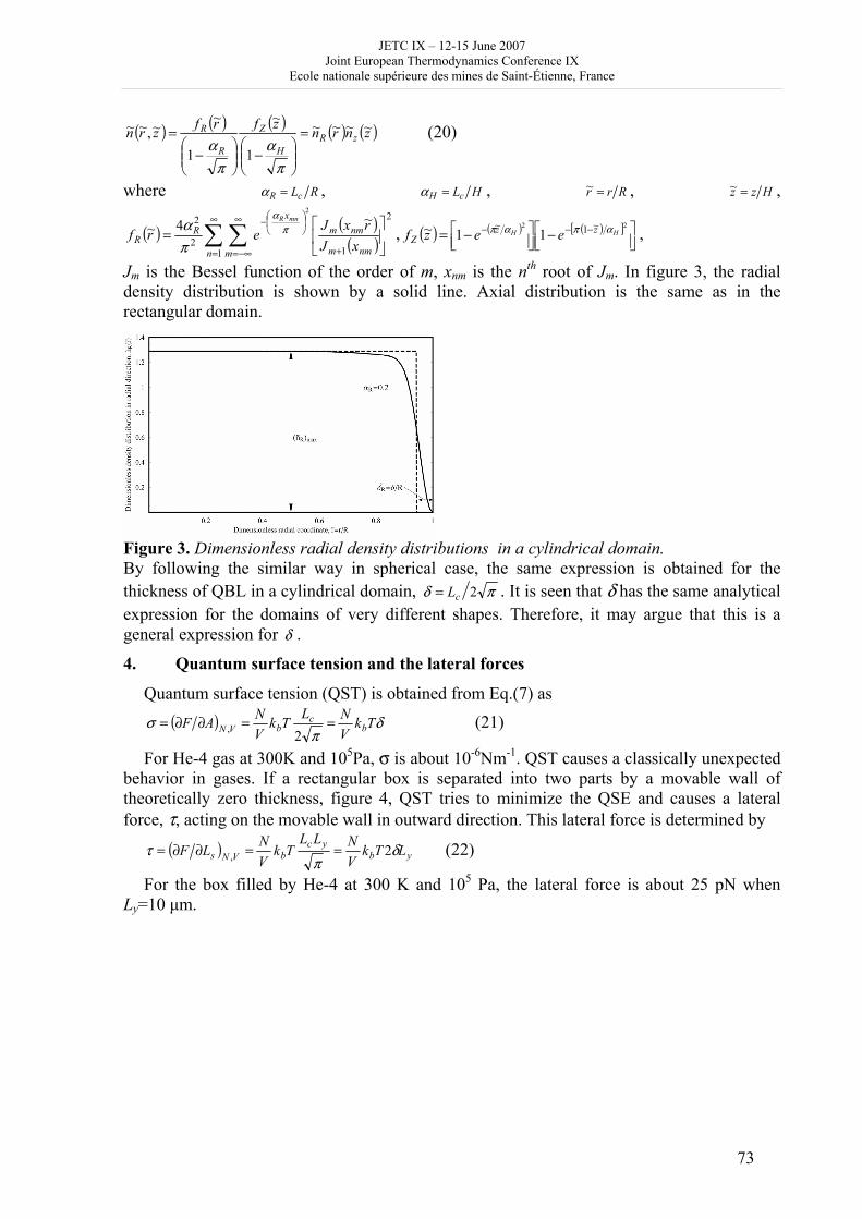
JETC IX – 12-15 June 2007 Joint European Thermodynamics Conference IX
Ecole nationale supérieure des mines de Saint-Étienne, France
73
( ) ( ) ( ) ( ) ( )znrnzfrfzrn zRH
Z
R
R ~~~~
1
~
1
~~,~~ =
⎟⎟⎠
⎞⎜⎜⎝
⎛−⎟⎟
⎠
⎞⎜⎜⎝
⎛−
=
πα
πα
(20)
where RLcR =α , HLcH =α , Rrr =~ , Hzz =~ ,
( ) ( )( )∑ ∑
∞
=
∞
−∞= +
⎟⎠⎞
⎜⎝⎛−
⎥⎦
⎤⎢⎣
⎡=
1
2
12
2 ~4~2
n m nmm
nmmx
RR xJ
rxJerf
mnR
πα
πα , ( ) ( ) ( )[ ]
⎥⎦⎤
⎢⎣⎡ −⎥⎦⎤
⎢⎣⎡ −= −−− 22 ~1~
11~ HH zzZ eezf απαπ ,
Jm is the Bessel function of the order of m, xnm is the nth root of Jm. In figure 3, the radial density distribution is shown by a solid line. Axial distribution is the same as in the rectangular domain.
Figure 3. Dimensionless radial density distributions in a cylindrical domain. By following the similar way in spherical case, the same expression is obtained for the thickness of QBL in a cylindrical domain, πδ 2cL= . It is seen that δ has the same analytical expression for the domains of very different shapes. Therefore, it may argue that this is a general expression for δ .
4. Quantum surface tension and the lateral forces
Quantum surface tension (QST) is obtained from Eq.(7) as ( ) δ
πσ Tk
VNLTk
VNAF b
cbVN ==∂∂=
2, (21)
For He-4 gas at 300K and 105Pa, σ is about 10-6Nm-1. QST causes a classically unexpected behavior in gases. If a rectangular box is separated into two parts by a movable wall of theoretically zero thickness, figure 4, QST tries to minimize the QSE and causes a lateral force, τ, acting on the movable wall in outward direction. This lateral force is determined by
( ) ybyc
bVNs LTkVNLL
TkVNLF δ
πτ 2, ==∂∂= (22)
For the box filled by He-4 at 300 K and 105 Pa, the lateral force is about 25 pN when Ly=10 μm.
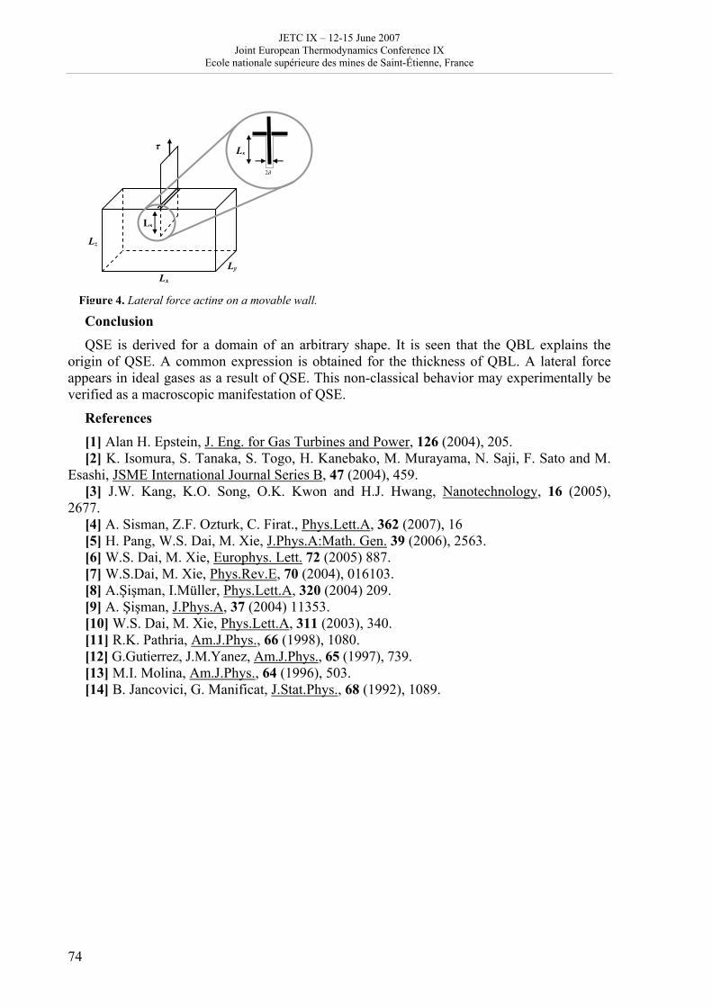
JETC IX – 12-15 June 2007 Joint European Thermodynamics Conference IX
Ecole nationale supérieure des mines de Saint-Étienne, France
74
Figure 4. Lateral force acting on a movable wall.
Conclusion QSE is derived for a domain of an arbitrary shape. It is seen that the QBL explains the
origin of QSE. A common expression is obtained for the thickness of QBL. A lateral force appears in ideal gases as a result of QSE. This non-classical behavior may experimentally be verified as a macroscopic manifestation of QSE.
References [1] Alan H. Epstein, J. Eng. for Gas Turbines and Power, 126 (2004), 205. [2] K. Isomura, S. Tanaka, S. Togo, H. Kanebako, M. Murayama, N. Saji, F. Sato and M.
Esashi, JSME International Journal Series B, 47 (2004), 459. [3] J.W. Kang, K.O. Song, O.K. Kwon and H.J. Hwang, Nanotechnology, 16 (2005),
2677. [4] A. Sisman, Z.F. Ozturk, C. Firat., Phys.Lett.A, 362 (2007), 16 [5] H. Pang, W.S. Dai, M. Xie, J.Phys.A:Math. Gen. 39 (2006), 2563. [6] W.S. Dai, M. Xie, Europhys. Lett. 72 (2005) 887. [7] W.S.Dai, M. Xie, Phys.Rev.E, 70 (2004), 016103. [8] A.Şişman, I.Müller, Phys.Lett.A, 320 (2004) 209. [9] A. Şişman, J.Phys.A, 37 (2004) 11353. [10] W.S. Dai, M. Xie, Phys.Lett.A, 311 (2003), 340. [11] R.K. Pathria, Am.J.Phys., 66 (1998), 1080. [12] G.Gutierrez, J.M.Yanez, Am.J.Phys., 65 (1997), 739. [13] M.I. Molina, Am.J.Phys., 64 (1996), 503. [14] B. Jancovici, G. Manificat, J.Stat.Phys., 68 (1992), 1089.
Ls
Lz
Lx Ly
τ
δ2
Ls
JETC IX – 12-15 June 2007 Joint European Thermodynamics Conference IX
Ecole nationale supérieure des mines de Saint-Étienne, France
75
Diffuse interface model for non-equilibrium phase transformations
Peter Galenko(1) and David Jou(2) (1)German Aerospace Center, Institute of Materials Physics in Space,
51170 Cologne, Germany (2)Departament de Fisica, Universitat Autonoma de Barcelona,
08193 Bellaterra, Catalonia, Spain;
[email protected] - [email protected] Diffuse-interface formalism is widely applied to phase transformations in condensed and soft media. The first introduction of the diffuse interface into the theory of phase transformations was made by Landau and Khalatnikov [1] by borrowing a formalism of the Landau theory of phase transitions [2]. Landau and Khalatnikov labeled different phases by an additional order parameter to describe anomalous sound absorption of liquid helium. In its well-known form, a formal variational approach was established by Ginzburg and Landau for the phase transitions from the normal to the superconducting phase [3]. A diffuse-interface model has also been developed for a description of phase transformations of the first order, especially for the solidification phenomenon [4-6].
The diffuse-interface model incorporates an order parameter in the form of a phase-field variable. The phase-field Φ has a constant value in homogeneous phases, e.g. Φ=-1 for an unstable phase. This phase is transformed into the stable phase with Φ=+1. Between these phases in the interfacial region, the phase field, Φ, changes steeply but smoothly from -1 to +1. Numerical solutions allow one to avoid explicit tracking of the interface and to locate the interface at Φ=0 [7]. The phase-field Φ is considered as an order parameter which is introduced to describe a moving interfacial boundary between unstable and stable phases. The main purpose of the present report is to describe a thermodynamically consistent model of rapid phase transformation in a binary system under local non-equilibrium conditions. Using the phase-field methodology, we derive governing equations compatible with the macroscopic formalism of extended irreversible thermodynamics [8]. The extended space of independent variables E is formed by the union of the classical set {C}={ Φ,, ce } consisting of the inner energy e , concentration c , and phase field variable Φ and of the additional space {F}={ qr , J
r, t∂Φ∂ / } consisting of the fast variables such as
fluxes of heat qr and solute Jr
, and also the rate of change t∂Φ∂ / of the phase-field variable. This yields
}/,,{},,{}{}{ tJqceFCE ∂Φ∂∪Φ=∪=rr . (1)
Our choice of fluxes as variables does not exclude other possibilities. For instance, one may formulate space {F} through the number of internal variables [9]. However, both descriptions based on introduction of fluxes and internal variables are compatible with each other through a Legendre transform.
In Eq. (1), fluxes qr and Jr
describe exchanges of heat and matter between the diffuse interface and the neighboring bulk phases. The fluxes do not follow instantaneously classical Fourier and Fick laws. It takes them some time (usually rather short) to reach the value predicted by the classical transport equations. Obviously, when the interface motion is fast
JETC IX – 12-15 June 2007 Joint European Thermodynamics Conference IX
Ecole nationale supérieure des mines de Saint-Étienne, France
76
enough, delay effects in the dynamics of fluxes may play a determining role. This happens, for instance, when the velocity V of the interface becomes comparable or higher than τ/l (where l being the mean-free-path of the particles and τ the relaxation time of fluxes). Thus, in these circumstances, qr and J
r behave as independent variables with their own dynamics,
which has important consequences for the dynamics and stability of the phase interface [10-12].
The introduction of t∂Φ∂ / as an additional independent variable is motivated by a similar, though slightly different consideration. Indeed, the space variation of Φ is related, among other factors, to the width of the interface. Thus, including t∂Φ∂ / as an independent variable allows for a more detailed description of both internal kinetics and shape of the interface. In the same way as in Newtonian mechanics (where the initial position and velocity of a particle must be specified to determine their evolution), here we take both Φ and t∂Φ∂ / as independent variables. If inertial effects are sufficiently low in comparison with dissipative effects, t∂Φ∂ / will be determined directly by a dynamical equation in terms of Φ and its gradient. Otherwise, Φ and t∂Φ∂ / will be independent and an equation for 22 / t∂Φ∂ must be found. To describe rapid phase transformation we use the following entropy functional:
Ω⎥⎥⎦
⎤
⎢⎢⎣
⎡Φ∇−∇−∇−∂Φ∂Φ= ∫Ω dcetJqcesS ce 2
22
22
2
222)/,,,,,( φεεεrr , (2)
where s is the entropy density based on the extended set (1) of independent thermodynamic variables, eε , cε , and φε constants for the energy, concentration, and phase-field, respectively. In the functional (2) the gradient terms are used to describe a spatial inhomogeneity within the fields according to previously formulated diffuse-interface models [3,7,13]. It is logical to include gradient terms in Eq. (2) because our interest is focused on interfaces with steep gradients. In addition to classic approach of Ginzburg and Landau [3], the entropy density s is based on the fluxes qr and J
r, and also adopts the rate of change
t∂Φ∂ / as the independent variable from the set (1). Entropy density s is an additive function of its local equilibrium contribution
),,( Φceseq and its pure non-equilibrium contribution )/,,( tJqsneq ∂Φ∂rr , i.e.
)/,,(),,()/,,,,,( tJqscestJqces neqeq ∂Φ∂+Φ=∂Φ∂Φ
rrrr . (3) Non-equilibrium contribution in Eq. (3) can be expanded in series as follows
( )222 )/(,,)(
)/,,( tJqOt
sJJsq
qstJqs
tneq ∂Φ∂+
∂Φ∂
Φ∂∂∂+
∂∂+
∂∂=∂Φ∂
rrrr
rr
rr . (4)
Taking linear proportionality for the derivatives: qqs q
rr α=∂∂ / , JJs J
rrα=∂∂ / , and
ts t ∂Φ∂=Φ∂∂∂ Φ /)(/ α , we omit terms with power of quadratic and higher order in the expansion (4). Then, Eq. (3) holds
JETC IX – 12-15 June 2007 Joint European Thermodynamics Conference IX
Ecole nationale supérieure des mines de Saint-Étienne, France
77
222
222),,()/,,,,,( ⎟
⎠⎞
⎜⎝⎛
∂Φ∂+++Φ=∂Φ∂Φ Φ
tJqcestJqces Jq
eqαααrr , (5)
where ,qα ,Jα and Φα are the coefficients independent on the fast variables
Eq. (5) shows that the entropy s has standard local equilibrium contribution eqs and contribution neqs explicitly dependent on fast variables. As it is well established in classic irreversible thermodynamics [14,15], thermodynamic functions (entropy, free energy, chemical potential) are strictly defined only for locally equilibrium states. Therefore, Eq. (5) can be specially explained by the following way. For the local equilibrium part eqs a local ergodicity (that is, the system needs to sample the phase space) is true. However, as soon as we postulate thermal and diffusion fluxes with their own finite relaxation times, as well as the rate t∂Φ∂ / of the phase-field change has its own finite relaxation time, this means that the local non-equilibrium contribution ( ) 2//2/2/ 222 tJq Jq ∂Φ∂++ Φααα assumes the existence of a slow physical processes, which are the thermal conduction and/or jump of solute atoms. Considering ergodicity of a phase space for non-equilibrium situation, one may well refer to statistical effects in fast phase transition due to the existence of many particles (atoms and molecules) within local volumes. Since we consider the phase transitions in high frequency approximation, the particles have not enough time to sample all the phase space. Thus, the number of microstates accessible to each of them will be lower than in equilibrium. This will imply a decrease in the entropy with respect to the local equilibrium contribution
eqs . This is one of the ways to interpret the non-equilibrium contribution neqs to the entropy (5). Using entropy density s in the form of Eq. (5), evolution of the total entropy (2) is described by the following system of equations [16] - the governing equation for energy density
⎥⎦
⎤⎢⎣
⎡⎟⎠⎞
⎜⎝⎛ ∇+
∂∂⋅∇⋅−∇=
∂∂+
∂∂ e
esM
te
te
eeT22
2
2
ετ , (6)
- the governing equation for solute concentration
⎥⎦
⎤⎢⎣
⎡⎟⎠⎞
⎜⎝⎛ ∇+
∂∂⋅∇⋅−∇=
∂∂+
∂∂ c
csM
tc
tc
ccD22
2
2
ετ , (7)
- the governing equation for the phase-field
⎟⎠⎞
⎜⎝⎛ Φ∇+
Φ∂∂∇=
∂Φ∂+
∂Φ∂
ΦΦ22
2
2
φετ sMtt
, (8)
where Tτ is the relaxation time for the heat diffusion flux, Dτ the relaxation time for solute diffusion flux, and Φτ is the timescale of the rate t∂Φ∂ / of phase-field change. According to Eq. (5), the acceleration 22 / t∂Φ∂ of the phase-field appears due to the introduction of both Φ and t∂Φ∂ / as independent variables. The acceleration characterizes inertial effects inside the width of diffuse interface.
In equations (6)-(8) one role of the relaxation times is clear: they characterize the delay with which qr and solute J
r reduce to their classical forms (which correspond to the
JETC IX – 12-15 June 2007 Joint European Thermodynamics Conference IX
Ecole nationale supérieure des mines de Saint-Étienne, France
78
classical transport equations). Furthermore, this delay indicates a loss of inertial effects in the dynamics of the interfacial region. Relaxation terms may be neglected in many circumstances, but become crucial in some important situations. For instance, they lead to a maximum possible value for the speed of advance of the interface (in contrast to the classic theory which allows for an infinite speed of propagation). Moreover, they lead to the possibility of oscillatory phenomena appearing within the domain of interface. Thus, the role of new terms is not simply to add some new undetermined parameters (i.e., the relaxation times), allowing for an improved fit with experimental results. These terms play an important conceptual role, because they open the possibility for a drastic change in behavior of the modeled system. Note that governing equations (6)-(8) describe the hyperbolic phase-field model. As an extension of this model, a model with memory, and a model of nonlinear evolution of transformation within the diffuse-interface can be developed [16]. The consistency of the model (6)-(8) is proved by the verification of the validity on phenomenological and microscopic levels of description [16]. Particularly, it is shown that governing equations (6)-(8) yield a definite positive expression for the entropy production in full agreement with the second law of thermodynamics. Also, our macroscopic formalism is consistent with the microscopic fluctuation-dissipation theorem. It has been shown that the transport coefficients (thermal conductivity, diffusion coefficient) are obtained in a form of well-known Green-Kubo formulae for transport coefficients [17-19]. It provides, in fact, a phenomenological complement to outcomes extracted from the fluctuation-dissipation theorem. The derived equations (6)-(8) for an evolution of diffuse interface are correlated with existing models of non-equilibrium transport processes and for the systems experiencing phase transformations. Particularly, they are compared with the outcomes following from models of superconductivity, viscoelastic or electronically-conducting fluids, interface motion by mean curvature, and reaction-diffusion systems. In the present report, we analyze solutions of the system (6)-(8) for rapidly solidifying systems and phase separation process by spinodal decomposition. Reasons for application of the present diffuse-interface model to processes of rapid solidification and spinodal decomposition are the following. At deep supercoolings in a solidifying system, or at high velocities of the solid-liquid interface, it is necessary to take into account local non-equilibrium effects in solute diffusion phenomena and to use a non-Fickian model for transport processes compatible with the extended irreversible thermodynamics [10-12]. The phenomenon of an advancement of diffuse-interfaces with higher velocities comparable with the solute diffusion speed is described by the phase-field model with a relaxation of the diffusion flux [20]. For systems rapidly quenched or deeply supercooled into the spinodal region or a phase diagram, the present diffuse-interface model is also applicable. The time for instability and transition from unstable state to the next metastable state under phase separation is very short and it is comparable with the time for relaxation of the solute diffusion flux. As a result, a partial differential equation of hyperbolic type (4) follows from the analysis of rapidly phase-separated systems. The predicted solutions for binary solidifying systems and phase-separated systems are tested against experimental data. References [1] L.D. Landau and I.M. Khalatnikov, Dokl. Akad. Nauk SSSR 96, 469 (1954); see also D. ter Haar (Editor): Collected Papers of L.D. Landau (Pergamon Press, Oxford, 1965), p.626. [2] L.D. Landau, JETP 7, 19 (1937); see also D. ter Haar (Editor): Collected Papers of L.D. Landau (Pergamon Press, Oxford, 1965), p.193.
JETC IX – 12-15 June 2007 Joint European Thermodynamics Conference IX
Ecole nationale supérieure des mines de Saint-Étienne, France
79
[3] V.L. Ginzburg and L.D. Landau, JETP 20, 1064 (1950); see also D. ter Haar (Editor): Collected Papers of L.D. Landau (Pergamon Press, Oxford, 1965), p.546. [4] G.J. Fix, in: Free Boundary Problems: Theory and Applications, Eds. A. Fasano and M. Primicerio (Pitman, Boston, 1983) p. 580. [5] J.B. Collins and H. Levine, Phys. Rev. B 31, 6119 (1985). [6] J.S. Langer, in: Directions in Condensed Matter Physics, Eds. G. Grinstein and G. Mazenko (World Scientific, Philadelphia, 1986) p. 165. [7] W.J. Boettinger, J.A. Warren, C. Beckermann, and A. Karma, Rev. Mater. Res. 32, 163 (2002). [8] D. Jou, J. Casas-Vazquez, and G. Lebon, Extended Irreversible Thermodynamics (Springer, Berlin, 1996). [9] D. Jou, J. Casas-Vazquez, and M. Criado-Sancho, Thermodynamics of Fluids Under Flow (Springer, Berlin, 2001). [10] P.K. Galenko and D.A. Danilov, Phys. Lett. A 278, 129 (2000). [11] P.K. Galenko and D.A. Danilov, J. Cryst Growth 216, 512 (2000). [12] P.K. Galenko and D.A. Danilov, Phys. Rev. E 69, 051608 (2004). [13] S.E. Allen and J.W. Cahn, Acta Metall. 27, 1085 (1979). [14] I. Progogine, Introduction to Thermodynamics of Irreversible Process (Interscience, New York, 1967). [15] P. Glansdorff and I. Prigogine, Thermodynamic Theory of Structure, Stability and Fluctuations (Wiley, New York, 1971). [16] P. Galenko and D. Jou, Phys. Rev. E 71, 046125 (2005). [17] P. Resibois and M. de Leener, Classical Kinetic Theory of Fluids (Wiley, New York, 1977). [18] D.N. Zubarev, V. Morozov, and G. Röpke, Statistical Mechanics of Nonequilibrium Processes (2 volumes), (Akademie Verlag, Berlin, 1977). [19] R. Luzzi, A.R. Vasconcellos, and J.G. Ramos, Foundation of a Nonequilibrium Ensemble Formalism (Kluwer, Dordrecht, 2002). [20] P. Galenko, Phys. Lett. A 287, 190 (2001).
JETC IX – 12-15 June 2007 Joint European Thermodynamics Conference IX
Ecole nationale supérieure des mines de Saint-Étienne, France
80
Local non-equilibrium effect on spinodal decomposition in a binary system
Peter Galenko(1) and Vladimir Lebedev(2) (1)German Aerospace Center, Institute of Materials Physics in Space,
51170 Cologne, Germany e-mail: (2)Udmurt State University, Department of Theoretical Physics,
426034 Izhevsk, Russia
[email protected] - [email protected] A phase transition in which both phases have equivalent symmetry but differ only in composition is well-known as spinodal decomposition. This transition has been theoretically described by Cahn and Hilliard [1,2] and experimentally tested within the context of critical phenomena on the Ground and in Space [3]. In parallel with detailed analysis and tests against experimental data the theory of Cahn and Hilliard has been further explored and developed. In particular, it has been shown that the theory has problems with the description of the early stages of decomposition. It has been demonstrated that experimental data extracted from light and x-ray scattering by phase-separated glasses [4,5] exhibit non-linear behavior in dispersion relation in contradiction with predictions of the Cahn-Hillard theory. According to the theory, only systems with long-range interaction may behave linearly during the early stage of spinodal decomposition [6]. This theoretical result has not been observed experimentally in systems with short-range interaction because non-linear or non-equilibrium effects become important for systems rapidly quenched or deeply supercooled into the spinodal region of a phase diagram. Recently, Cahn-Hillard theory has been modified by taking into account the relaxation of diffusion flux to its local steady state [7,8]. Using methods of extended irreversible thermodynamics, a partial differential equation of a hyperbolic type
( )[ ]cfMtc
tc
ccD22'
2
2
∇−∇⋅∇=∂∂+
∂∂ ετ
for phase separation with diffusion has been derived that can be called ``a hyperbolic model for spinodal decomposition''. In the above equation the following notations are introduced: c is the concentration, t the time, Dτ the relaxation time for diffusion flux to its steady state, M the atomic mobility, '
cf the derivative of the free energy density with respect to concentration, cε is the factor proportional to the correlation length.
In the present report, analysis of this hyperbolic model is given to predict critical parameters of decomposition in comparison with the outcomes of the Cahn-Hilliard theory. The dynamics of spinodal decomposition is modelled in 1D and 3D using computational methods of solution of the hyperbolic and parabolic differential equations. From the analytical treatments it is shown that the hyperbolic model predicts non-linearity in the amplification rate of decomposition, which is governed by the ratio between diffusion length and correlation length. The predicted amplification rate is tested against experimental data on a binary phase-separated glass.

JETC IX – 12-15 June 2007 Joint European Thermodynamics Conference IX
Ecole nationale supérieure des mines de Saint-Étienne, France
81
References [1] J.W. Cahn and J.E. Hilliard, J. Chem. Phys. 28, 258 (1958). [2] J.W. Cahn, Acta Metall. 9, 795 (1961). [3] D. Beysens, In: Materials Sciences in Space. Edited by B. Feuerbacher, H. Hamacher and R.J. Naumann (Springer, Berlin, 1986) pp. 191-224. [4] N.S. Andreev, G.G. Boiko, and N.A. Bokov, J. Non-Cryst. Solids 5, 41 (1970) [5] N.S. Andreev and E.A. Porai-Koshits, Discuss. Faraday Soc. 50, 135 (1970). [6] K. Binder and P. Fratzl, In: Phase transformations in materials. Edited by G. Kostorz (Wiley, Weinheim, 2001), pp. 409-480. [7] P. Galenko, Phys. Lett. A 287, 190 (2001). [8] P. Galenko and D. Jou, Phys. Rev. E 71, 046125 (2005).
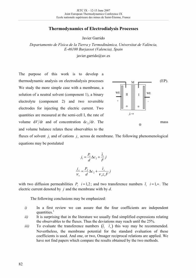
JETC IX – 12-15 June 2007 Joint European Thermodynamics Conference IX
Ecole nationale supérieure des mines de Saint-Étienne, France
82
Thermodynamics of Electrodialysis Processes
Javier Garrido
Departamento de Física de la Tierra y Termodinámica, Universitat de València, E-46100 Burjassot (Valencia), Spain
[email protected] The purpose of this work is to develop a
thermodynamic analysis on electrodialysis processes (EP).
We study the more simple case with a membrane, a
solution of a neutral solvent (component 1), a binary
electrolyte (component 2) and two reversible
electrodes for injecting the electric current. Two
quantities are measured at the semi-cell I, the rate of
volume dV dt and of concentration dc2 dt . The mass
and volume balance relates these observables to the
fluxes of solvent j1 and of cations j+ across de membrane. The following phenomenological
equations may be postulated
j1 = P1
dΔc2 + t 1
Fj
j+
ν +
= P2
dΔc2 + t +
ν +z+Fj
with two diffusion permeabilities Pi i =1,2 ; and two transference numbers t i i =1,+ . The electric current denoted by j and the membrane with by d.
The following conclusions may be emphasized:
i) In a first review we can assure that the four coefficients are independent quantities.1
ii) It is surprising that in the literature we usually find simplified expressions relating the observables to the fluxes. Thus the deviations may reach until the 25%.
iii) To evaluate the transference numbers t 1 t +( ) this way may be recommended. Nevertheless, the membrane potential for the standard evaluation of these coefficients is used. And one, or two, Onsager reciprocal relations are applied. We have not find papers which compare the results obtained by the two methods.
II I
+ -
WE WE
ji→
M
⊗⊗
⊗
JETC IX – 12-15 June 2007 Joint European Thermodynamics Conference IX
Ecole nationale supérieure des mines de Saint-Étienne, France
83
iv) The EP are better characterized by the electric current than by the electric potential ψ . In thermodynamics the electric equilibrium is better expressed by j = 0 than by ψ constant.2
v) The electric potential is measured at the terminals of the electrodes and always is an observable quantity.2 This variable plays a complementary role in EP.
vi) Profiles of the chemical and electrochemical potentials explain well the transport of the constituents across the membrane.
1. J. Garrido, Transport Equations of Electrodiffusion Processes in the Laboratory Reference Frame; J. Phys. Chem. B, 110, 3276 (2006). 2. J. Garrido, Thermodynamics of Electrochemical Systems; J. Phys. Chem. B, 108, 18336 (2004).
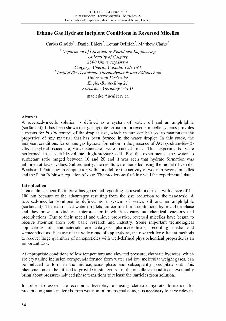
JETC IX – 12-15 June 2007 Joint European Thermodynamics Conference IX
Ecole nationale supérieure des mines de Saint-Étienne, France
84
Ethane Gas Hydrate Incipient Conditions in Reversed Micelles
Carlos Giraldo1 , Daniel Ehlers2, Lothar Oellrich2, Matthew Clarke1 1 Department of Chemical & Petroleum Engineering
University of Calgary 2500 University Drive
Calgary, Alberta, Canada, T2N 1N4 2 Institut für Technische Thermodynamik und Kältetechnik
Universität Karlsruhe Engler-Bunte-Ring 21
Karlsruhe, Germany, 76131
[email protected] Abstract A reversed-micelle solution is defined as a system of water, oil and an amphilphile (surfactant). It has been shown that gas hydrate formation in reverse-micelle systems provides a means for in-situ control of the droplet size, which in turn can be used to manipulate the properties of any material that has been formed in the water droplet. In this study, the incipient conditions for ethane gas hydrate formation in the presence of AOT(sodium-bis-(2-ethyl-hexyl)sulfosuccinate)-water-isooctane were carried out. The experiments were performed in a variable-volume, high-pressure cell. For the experiments, the water to surfactant ratio ranged between 10 and 20 and it was seen that hydrate formation was inhibited at lower values. Subsequently, the results were modelled using the model of van der Waals and Platteeuw in conjunction with a model for the activity of water in reverse micelles and the Peng Robinson equation of state. The predictions fit fairly well the experimental data. Introduction Tremendous scientific interest has generated regarding nanoscale materials with a size of 1 - 100 nm because of the advantages resulting from the size reduction to the nanoscale. A reversed-micellar solutions is defined as a system of water, oil and an amphilphile (surfactant). The nano-sized water droplets are confined in a continuous hydrocarbon phase and they present a kind of microreactor in which to carry out chemical reactions and precipitations. Due to their special and unique properties, reversed micelles have begun to receive attention from both basic research and industry. Some important technological applications of nanomaterials are catalysis, pharmaceuticals, recording media and semiconductors. Because of the wide range of applications, the research for efficient methods to recover large quantities of nanoparticles with well-defined physiochemical properties is an important task. At appropriate conditions of low temperature and elevated pressure, clathrate hydrates, which are crystalline inclusion compounds formed from water and low molecular weight gases, can be induced to form in the microaqueous phase and subsequently precipitate out. This phenomenon can be utilised to provide in-situ control of the micelle size and it can eventually bring about pressure-induced phase transitions to release the particles from solution. In order to assess the economic feasiblity of using clathrate hydrate formation for precipitating nano-materials from water-in-oil microemulsions, it is necessary to have relevant
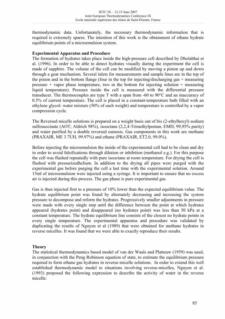
JETC IX – 12-15 June 2007 Joint European Thermodynamics Conference IX
Ecole nationale supérieure des mines de Saint-Étienne, France
85
thermodynamic data. Unfortunately, the necessary thermodynamic information that is required is extremely sparse. The intention of this work is the obtainment of ethane hydrate equilibrium points of a microemulsion system. Experimental Apparatus and Procedure The formation of hydrates takes place inside the high-pressure cell described by Dholabhai et al. (1996). In order to be able to detect hydrates visually during the experiment the cell is made of sapphire. The volume of the cell can be modified by moving a piston up and down through a gear mechanism. Several inlets for measurements and sample lines are in the top of the piston and in the bottom flange (four in the top for injecting/discharging gas + measuring pressure + vapor phase temperature, two in the bottom for injecting solution + measuring liquid temperature). Pressure inside the cell is measured with the differential pressure transducer. The thermocouples are type T with a span from -60 to 90°C and an inaccuracy of 0.5% of current temperature. The cell is placed in a constant-temperature bath filled with an ethylene glycol- water mixture (50% of each weight) and temperature is controlled by a vapor compression cycle. The Reversed micelle solutions is prepared on a weight basis out of bis (2-ethylhexyl) sodium sulfosuccinate (AOT; Aldrich 98%), isooctane (2,2,4-Trimethylpentan, EMD; 99,95% purity) and water purified by a double reversed osmosis. Gas components in this work are methane (PRAXAIR, ME 3.7UH, 99.97%) and ethane (PRAXAIR, ET2.0, 99.0%). Before injecting the microemulsion the inside of the experimental cell had to be clean and dry in order to avoid falsifications through dilution or inhibition (methanol e.g.). For this purpose the cell was flushed repeatedly with pure isooctane at room temperature. For drying the cell is flushed with pressurizedhelium. In addition to the drying all pipes were purged with the experimental gas before purging the cell a last time with the experimental solution. Around 15ml of microemulsion were injected using a syringe. It is important to ensure that no excess air is injected during this process. The gas phase is pure experimental gas. Gas is then injected first to a pressure of 10% lower than the expected equilibrium value. The hydrate equilibrium point was found by alternately decreasing and increasing the system pressure to decompose and reform the hydrates. Progressively smaller adjustments in pressure were made with every single step until the difference between the point at which hydrates appeared (hydrates point) and disappeared (no hydrates point) was less than 50 kPa at a constant temperature. The hydrate equilibrium line consists of the closest no hydrate points in every single temperature. The experimental apparatus and procedure was validated by duplicating the results of Nguyen et al (1989) that were obtained for methane hydrates in reverse micelles. It was found that we were able to exactly reproduce their results. Theory The statistical thermodynamics based model of van der Waals and Platteuw (1959) was used, in conjunction with the Peng Robinson equation of state, to estimate the equilibrium pressure required to form ethane gas hydrates in reverse-micelle solutions. In order to extend this well established thermodynamic model to situations involving reverse-micelles, Nguyen et al. (1993) proposed the following expression to describe the activity of water in the reverse micelle:
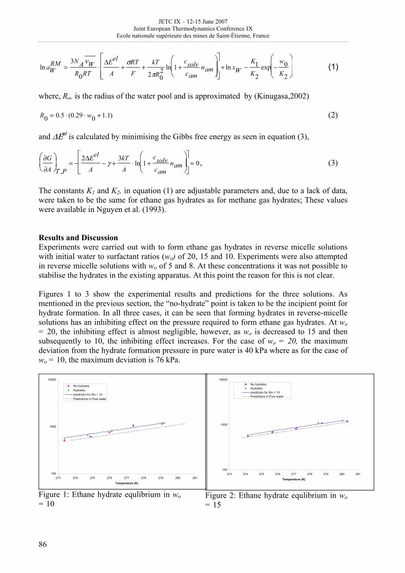
JETC IX – 12-15 June 2007 Joint European Thermodynamics Conference IX
Ecole nationale supérieure des mines de Saint-Étienne, France
86
ln aWRM =
3N A νWR0RT
⋅ΔEel
A+
σRT
F+
kT
2πR02 ln 1 +
csolvcam
nam⎛
⎝ ⎜
⎞
⎠ ⎟
⎡
⎣ ⎢ ⎢
⎤
⎦ ⎥ ⎥
+ ln xW −K1K2
exp −w0K2
⎛
⎝ ⎜ ⎜
⎞
⎠ ⎟ ⎟ (1)
where, Ro, is the radius of the water pool and is approximated by (Kinugasa,2002) R0 = 0.5 ⋅ (0.29 ⋅ w0 + 1.1) (2) and ΔΕel is calculated by minimising the Gibbs free energy as seen in equation (3),
∂G
∂A
⎛ ⎝ ⎜
⎞ ⎠ ⎟ T ,P
= −2ΔEel
A− γ +
3kT
A⋅ ln 1 +
csolvcam
nam⎛
⎝ ⎜
⎞
⎠ ⎟
⎡
⎣ ⎢
⎤
⎦ ⎥ = 0, (3)
The constants K1 and K2, in equation (1) are adjustable parameters and, due to a lack of data, were taken to be the same for ethane gas hydrates as for methane gas hydrates; These values were available in Nguyen et al. (1993). Results and Discussion Experiments were carried out with to form ethane gas hydrates in reverse micelle solutions with initial water to surfactant ratios (wo) of 20, 15 and 10. Experiments were also attempted in reverse micelle solutions with wo of 5 and 8. At these concentrations it was not possible to stabilise the hydrates in the existing apparatus. At this point the reason for this is not clear. Figures 1 to 3 show the experimental results and predictions for the three solutions. As mentioned in the previous section, the “no-hydrate” point is taken to be the incipient point for hydrate formation. In all three cases, it can be seen that forming hydrates in reverse-micelle solutions has an inhibiting effect on the pressure required to form ethane gas hydrates. At wo = 20, the inhibiting effect is almost negligible, however, as wo is decreased to 15 and then subsequently to 10, the inhibiting effect increases. For the case of wo = 20, the maximum deviation from the hydrate formation pressure in pure water is 40 kPa where as for the case of wo = 10, the maximum deviation is 76 kPa.
100
1000
10000
273 274 275 276 277 278 279 280 281
Temperature (K)
No hydratesHydratesprediction for Wo = 10Predictions in Pure water
Figure 1: Ethane hydrate equlibrium in wo = 10
100
1000
10000
273 274 275 276 277 278 279 280 281
Temperature (K)
No hydratesHydratesprediction for Wo = 15Predictions in Pure water
Figure 2: Ethane hydrate equlibrium in wo = 15
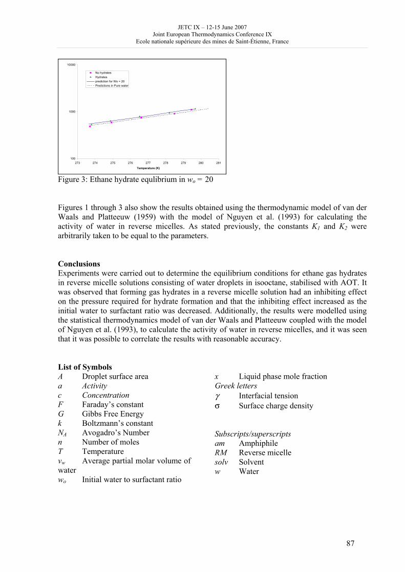
JETC IX – 12-15 June 2007 Joint European Thermodynamics Conference IX
Ecole nationale supérieure des mines de Saint-Étienne, France
87
100
1000
10000
273 274 275 276 277 278 279 280 281
Temperature (K)
No hydratesHydratesprediction for Wo = 20Predictions in Pure water
Figure 3: Ethane hydrate equlibrium in wo = 20 Figures 1 through 3 also show the results obtained using the thermodynamic model of van der Waals and Platteeuw (1959) with the model of Nguyen et al. (1993) for calculating the activity of water in reverse micelles. As stated previously, the constants K1 and K2 were arbitrarily taken to be equal to the parameters. Conclusions Experiments were carried out to determine the equilibrium conditions for ethane gas hydrates in reverse micelle solutions consisting of water droplets in isooctane, stabilised with AOT. It was observed that forming gas hydrates in a reverse micelle solution had an inhibiting effect on the pressure required for hydrate formation and that the inhibiting effect increased as the initial water to surfactant ratio was decreased. Additionally, the results were modelled using the statistical thermodynamics model of van der Waals and Platteeuw coupled with the model of Nguyen et al. (1993), to calculate the activity of water in reverse micelles, and it was seen that it was possible to correlate the results with reasonable accuracy. List of Symbols A Droplet surface area a Activity c Concentration F Faraday’s constant G Gibbs Free Energy k Boltzmann’s constant NA Avogadro’s Number n Number of moles T Temperature vw Average partial molar volume of water wo Initial water to surfactant ratio
x Liquid phase mole fraction Greek letters γ Interfacial tension σ Surface charge density Subscripts/superscripts am Amphiphile RM Reverse micelle solv Solvent w Water
JETC IX – 12-15 June 2007 Joint European Thermodynamics Conference IX
Ecole nationale supérieure des mines de Saint-Étienne, France
88
Acknowledgment This study was made possible with a generous grant from support from the Department of Chemical and Petroleum Engineering at the University of Calgary, with funding allocated from the Zandmer Estate. References
1. H.T. Nguyen, N. Kommareddy, V.T. John;A thermodynamic model to Predict Clathrate Hydrate Formation in Water-in-Oil Microemulsion Systems; Journal of colloid and interface Science 155, 482-487 (1993)
2. H.T. Nguyen, J.B. Phillips, V.T. John; Clathrate Hydrate Formation in reversed Micellar Solutions; The journal of physical chemistry Vol. 93, No. 25, 8123-8126, (1989)
3. J.B. Phillips, H. Nguyen, V.T. John; Protein Recovery from Reversed Micellar Solutions through Contact with a Pressurized Gas Phase; Biotechnol. Prog., Vol. 7, 43-48, (1991)
4. A.M. Rao, H. Nguyen, V.T. John; Modification of Enzyme Activity in Reversed Micelles through Clathrate Hydrate Formation; Biotchnol. Prog. Vol. 6, 465-471, (1990).
5. Dholabhai, P.D., Parent, J.S., Bishnoi, P.R.; Carbon Dioxide Hydrate Equilibrium in Aqueous Conditions Containing Electrolytes and Methanol using a New Apparatus; Ind. Eng. Chem. Res., Vol. 35, 819 – 826, (1996).
6. Van der Waals, J.H., Platteeuw, J.C., Clathrate Solutions, Adv.Chem.Phys., 2(1), 1-57, (1959).
7. T Kinugasa, A Kondo, S. Nishimura, Y Miyauchi, Y. Nishii, K. Watanabe, H Takeuchi. Estimation for size of reverse micelles formed by AOT and SDEHP based on viscosity measurement, Colloids and Surfaces A Vol 204, 193-199, (2002)
JETC IX – 12-15 June 2007 Joint European Thermodynamics Conference IX
Ecole nationale supérieure des mines de Saint-Étienne, France
89
Influence of heating substrate geometry and humidity on the dynamics of evaporating sessile water droplets
Fabien Girarda, Mickaël Antonia, Sylvain Faureb and Annie Steinchen-Sanfelda a Laboratoire de Thermodynamique et de Modélisation des Milieux hors Equilibre, UMR-CNRS 6171, Université Paul Cézanne Aix-Marseille BP 451, F-13397, Marseille cedex 20
(France) b CEA-Marcoule, Laboratoire des Procédés Avancés de Décontamination,
DTCD/SPDE/LPAD, Bât. 222, F-30207 Bagnols/Cèze Cedex (France)
[email protected] Evaporating systems have for long interested both the academic and industrial community. Specific properties like hydrodynamical instabilities, coexisting vapor-fluid phases and the role of interfaces have been investigated and used in various fields of industrial applications (paintings, cooling systems, printers and photocopiers, etc). The complete understanding of evaporation phenomena still motivates important scientific activity. One important objective is, for example, to allow substrate characterization from measured evaporation rates or contact angle dynamics. We propose to investigate numerically the properties of water evaporating droplets on a heating substrate [1]. These droplets are assumed to be sessile and axi-symmetric for the duration of the evaporation process. The dynamics is described through the usual hydrodynamic equations and the coupling between the droplet and surrounding air is determined by the water diffusivity in air, the rate of humidity and the local vapor pressure. We compare the numerical outputs with experimental data [2, 3] and show a relative good agreement. We investigate the influence of the heating substrate on evaporation dynamics [4] and describe the evolution of the Marangoni velocity field on the free interface [5]. We also present results about the role of humidity rate. We finally discuss the influence of the size of the heating substrate on droplet evaporation dynamics. [1] Hu, H. and Larson, R. G. Langmuir, 21 (2005), 3963-3971 [2] Crafton, E. F. and Black, W. Z. Int. J. Heat Mass Transfer, 47 (2004) 1187-1200 [3] Sefiane, K, J. Petrol. Sci. Eng. 51 (2006), 238-252 [4] Girard, F. et al. Microgravity Sci. Technol. 18(3/4), (2006) 42-46 [5] Girard, F. et al. Langmuir, (in press)
JETC IX – 12-15 June 2007 Joint European Thermodynamics Conference IX
Ecole nationale supérieure des mines de Saint-Étienne, France
90
Prigogine and the time problem: a dialog between physics and philosophy
Bernard GUY
Ecole nationale supérieure des mines de Saint-Etienne, France
[email protected] As many researchers did before him, Prigogine remained interested during his whole life by the time problem. It is useful to distinguish between two wordings: 1) the philosophical problem: "Time does not go backwards, why?" and 2) the physico-mathematical problem: "How can one go from the microscopic laws of mechanics, that are reversible by changing the direction of the parameter t: f (t) = f (-t), to the macroscopic laws of thermodynamics, that are irreversible: g(t) ≠ g (-t)?". A number of solutions have been proposed for problem (2). They are based on the “practical” resolution of the equations of mechanics for systems with a large (huge) number of particles: one loses the link with the initial conditions, owing to a number of effects associated to the instabilities, to the sensitiveness to the initial conditions known with a limited precision, to perturbations of different kinds, to the fractal character of the trajectories etc. One then needs an approach requiring the use of probabilities and irreversible equations of master equation or Boltzmann equation type. In this framework, one cannot go backwards because the initial conditions that would allow the return are improbable (impossible to prepare; see recent synthesis by Bricmont). Prigogine does not discuss the mathematical validity of these solutions and stands on the philosophical point of view (problem (1)) while saying: "- No, we cannot accept that the irreversibility of time, that raises as an elementary observation of nature, is linked to our ignorance or to an approximation of our representations". Prigogine and collaborators focus their work on the nonintegrable Poincaré systems with continuous spectrum which lead to the appearance of diffusive terms in the framework of dynamics, terms that break time symmetry and that are amplified. As a result one has to include already in the fundamental dynamical description the two aspects, probability and irreversibility. This approach, that is based on a continuous description of the equations of mechanics (phase spaces) is a new solution to problem (2) but, according to us, does not constitute the solution of the general problem (1). As a matter of fact, it still deals with systems with a large number of degrees of freedom and rather reveals a property of the number of particles of these systems than of time itself. How can one understand that time be able or not to go backwards "alone", regardless the world itself, that is regardless the number and the movement of the particles of a system? To ask this question, this is to stand at the philosophical level and at the joint between the philosophical level and the mathematical level. In these conditions, the first problem of time is not its irreversibility but more fundamentally its existence, that is to say its existence "alone". In reality, we do not study the properties of time alone, we construct it, and we construct it as opposed to space. This is done by taking into account the opposed relations of mobility and immobility of the material points. This opposition is not given once for ever but contains an irreducible part of approximation. The solution of the new problem we set, that can only be sketched here, is therefore equivalent to say: time does not exist alone, time is another manner to speak of space (as the theory of relativity also invites us to say). Time is associated to the relative mobility of the particles, space to their
JETC IX – 12-15 June 2007 Joint European Thermodynamics Conference IX
Ecole nationale supérieure des mines de Saint-Étienne, France
91
relative immobility, the two mobility and immobility concepts cannot be thought of separately. The opposition between reversibility and irreversibility is then based on this opposition and merely understood as the possible or impossible going back of some of the particles of the world with respect to others that would build the spatial frame for this potential return. Irreversibility and reversibility are then thought of in the same time and the limit between them is matter to approximation. As a conclusion, we are able to analyse how mathematical irreversibility increases with the number of particles of a system (decrease of the probability of the initial conditions allowing to go backward), knowing that an ontological or philosophical irreversibility, or rather a pair of associated reversibility and irreversibility concepts with an uncertain boundary provides the foundation of our thought of time. One retrieves the situation of an uncertain and open world as valued by Ilya Prigogine, but the uncertainty does not affect only the results of our investigation task, but the very tools of representation of the world, among which the opposition between time and space, or between reversibility and irreversibility.
JETC IX – 12-15 June 2007 Joint European Thermodynamics Conference IX
Ecole nationale supérieure des mines de Saint-Étienne, France
92
Geology and thermodynamics
Bernard GUY
Ecole nationale supérieure des mines de Saint-Etienne, France
[email protected] "This is to heat that the large movements that strike our eye upon the earth must be attributed; to it the agitations of the atmosphere, the ascension of the clouds, the fall of rains and other meteors, the watercourses that stream across the surface of the globe and a small part of which man succeeded to employ for his usage. At last, the earthquakes, the volcanic eruptions also recognize heat for their cause." Sadi Carnot (Reflections on the driving power of fire, 1824) Geology and thermodynamics are linked in both ways. Understood as upstream geology, thermodynamics certainly knows interesting applications in earth sciences. But cannot one envision the things the other way and note that the phenomena studied by geology furnished a motivation for the very construction of thermodynamics, as suggested by the above quote from Sadi Carnot at the beginning of his work? In our communication, we will choose some examples, largely drawn from our own research, where the comprehension work of the geological phenomena does not rest on a simple application of thermodynamics, but can enrich it and make it progress. For example: - Topological approaches to phase diagrams: the lack of thermodynamic data stimulated petrologists to take advantage of the sole composition of the phases in order to discuss the potential qualitative structure of phase diagrams. Original algebraic approaches were proposed (linear programming, theory of matroïds). - Study of systems with large dimensions: natural phenomena furnish new examples of dissipative structures on time and space scales with no comparison with those observed in the laboratory. They even give us the benefit of hindsight on our usual space and time variables! - Changes of scales: geology studies systems from the atomic scale to the scale of the continents. It is not evident that one can use the same laws or the same physical parameters to these different scales. The question therefore raises of the homogenization of the parameters and of the thermodynamic and kinetic laws. Certain phenomena at local scale (millimetre or centimetre scale), such as diffusion or kinetics, may be considered as negligible with respect to other phenomena to the metric or kilometric scale, such as those induced by convective movements. In order to describe these systems, hyperbolic type laws can be thus more adequate than parabolic type ones. The same phenomena show aspects of macroscopic quantification: the possible compositions form a discrete set and are selected by the second principle of the thermodynamics ("entropic condition" of hyperbolic problems). One can couple for them probabilistic approaches (which probability do we have to observe such rock composition?). - Study of complex systems, because of the number of components as well as the type of initial and boundary conditions (chemical variability of open systems). Today big computer
JETC IX – 12-15 June 2007 Joint European Thermodynamics Conference IX
Ecole nationale supérieure des mines de Saint-Étienne, France
93
codes are constructed in order to simulate phenomena to the geological scale, and are used for basic or applied research (CO2 storage). From a general point of view, before doing quantitative thermodynamic modelling, there remains not to underestimate the difficulty to unravel the complex history of the geological systems. Guy B. et Pla J.M. (1997) Structure of phase diagrams for n-component (n+k)-phase chemical systems: the concept of affigraphy, C. R. Acad. Sc. Paris, 324, IIa, 737-743. Guy B. (1981) Certain recurrent alternations of minerals in skarns and the dissipative structures in the sense of Prigogine: a parallel; C.R. Acad. Sc., Paris, 292, II, 413-416. Guy B. (2005) The behavior of solid solutions in geological transport processes : the quantization of rock compositions by fluid-rock interaction, in: Complex inorganic solids, structural, stability and magnetic properties of alloys, edited by P. Turchi, A. Gonis, K. Rajan and A. Meike, Springer, 265-273.
JETC IX – 12-15 June 2007 Joint European Thermodynamics Conference IX
Ecole nationale supérieure des mines de Saint-Étienne, France
94
Prediction of activity coefficients in non ideal solutions
S.L Hafsaoui, M. Ould Slimane and R. Mahmoud
Ecole Militaire Polytechnique, BP17, Bordj El Bahri, 16111, Algeria
Study of heavy hydrocarbon mixtures presents a practical advantage resulting from the importance of thermodynamic properties in the elaboration of many industrial processes. There is also a theoretical interest if we use statistical models to represent these strongly non ideal mixtures, according to energetic interactions and structure influence of these mixtures, on the thermodynamic properties. Prediction of thermodynamic properties of biphenyl in n-tetracosane, biphenyl in n-eicosane and dibenzofuran in n-octadecane is studied. Experimental results of liquid-solid equilibria (SLE) by means the differential scanning calorimeter (DSC) of these binaries, were used to estimate the influence of heteroatoms on polyaromatic structures interactions in solution with n-alkanes, and the corresponding activity coefficients were calculated using a group contribution method [1]. The three systems selected can be used for contributing to develop the data base using group contribution methods. For practical purposes, SLE are of interest in chemical process design, especially when process conditions must be specified to prevent solid deposition. We studied the phase behaviour of these binary solutions, and experimental results for these precursor systems are expected to supply information useful to characterising thermodynamics of phenomena occurring in heavy fractions of petroleum fluids, paraffin deposition, or flocculation. Most generally speaking, the flocculation results from interactions between the aromatic, polar part of the petroleum fluid with the non-polar, aliphatic environment. When these interactions become sufficiently important they allow liquid-liquid demixion accompanied by flocculation. In this study we discuss thermodynamic data concerning relatively simple systems which yield information on interactions leading to the above mentioned phenomena. Activity coefficients of components in systems containing long chain n-alkanes, can be estimated using Kehiaian model with parameters determined using experimental data [2]. Therefore, it was possible to obtain an interesting representation of these strongly non ideal systems. The influence of the presence of an heteroatom on the thermodynamic properties, can be explained by the steric and energetic environment of a group, which can possess an effect on interactions of this structure with groups of other molecules. This phenomenon still appears in a remarkable way in the case of polar molecules. Indeed, the interactions of a heteroatom with electronic structures of the polyaromatic cycles, modify the energetic situation of the groups constituting the molecule in mixture. References [1] H.V. Kehiaian, J.P. Grolier and G.C. Benson. Thermodynamics of organic mixtures. A generalized quasi chemical theory in term of group surface interactions. J. Chem. Phys., 75 (1978) 11-12. [2] J.A. Nelder, R. Mead. A simplex method for function minimization., Comp. J., (1965) 308-313.
JETC IX – 12-15 June 2007 Joint European Thermodynamics Conference IX
Ecole nationale supérieure des mines de Saint-Étienne, France
95
Quantifying Dissipative Processes
Karl Heinz Hoffmann1 1 Institut für Physik – Technische Universität Chemnitz – 09107 Chemnitz – Germany
[email protected] 1 Motivation and Introduction Real energy conversion processes are irreversible, and thus unavoidable losses occur as entropy is produced. These losses limit the efficiency of such processes and new bounds on the performance of heat engines appear. Equilibrium thermodynamics which compares real processes to reversible processes proceeding without losses at an infinite slow speed leads to a valid upper bound for efficiency. However it can not provide a sensible least upper bound for real irreversible processes and thus it may not be good enough to be a useful guide in the improvement of real processes. An example is the often used Carnot efficiency: HLC 1 TT−=η (1) It gives the fraction of the heat which at most can be converted to work in any engine using heat from a hot reservoir at temperature TH and rejecting some of the heat to a reservoir at lower temperature TL. Real heat engines, for example, seldom attain more than a fraction of the reversible Carnot efficiency. Engineers tried to diminish this discrepancy between real process and limiting reversible process by improving their design, specific to certain devices or processes. But despite all technological progress in engineering, the gap remains, and it has to remain due to the irreversible nature of real processes. Thus the remaining principle questions are “What are realistic bounds for thermodynamic processes performed in finite time?”' and “What are valid process paths to achieve this optimal process?”' This challenge has inspired scientists to conduct a wide spectrum of research activities. Already about fifty years ago the effect of finite heat transfer rates came into the focus of efficiency considerations for heat engines [1]. The effect of finite heat transfer on the power output of an otherwise reversible power plant was investigated. It was discovered that the efficiency at the maximum power point, HLC 1 TT−=η (2) is considerably lower than the corresponding Carnot efficiency. However, at that time this research activities did not attain much attention. After Curzon and Ahlborn 1975 re-discovered [2] the efficiency expression (2), which they found in remarkable agreement with the performance data of real power plants, the framework of finite time thermodynamics evolved (see for instance [3,4]). One reason was the oil crisis hitting the economy, again forcing the view on efficiency limiting irreversibilities of heat engines. The goal of this framework is to determine performance bounds for thermodynamic processes proceeding in a finite time or with finite rates. It has been applied since then mainly for thermal engines or processes. In general the approaches taken were
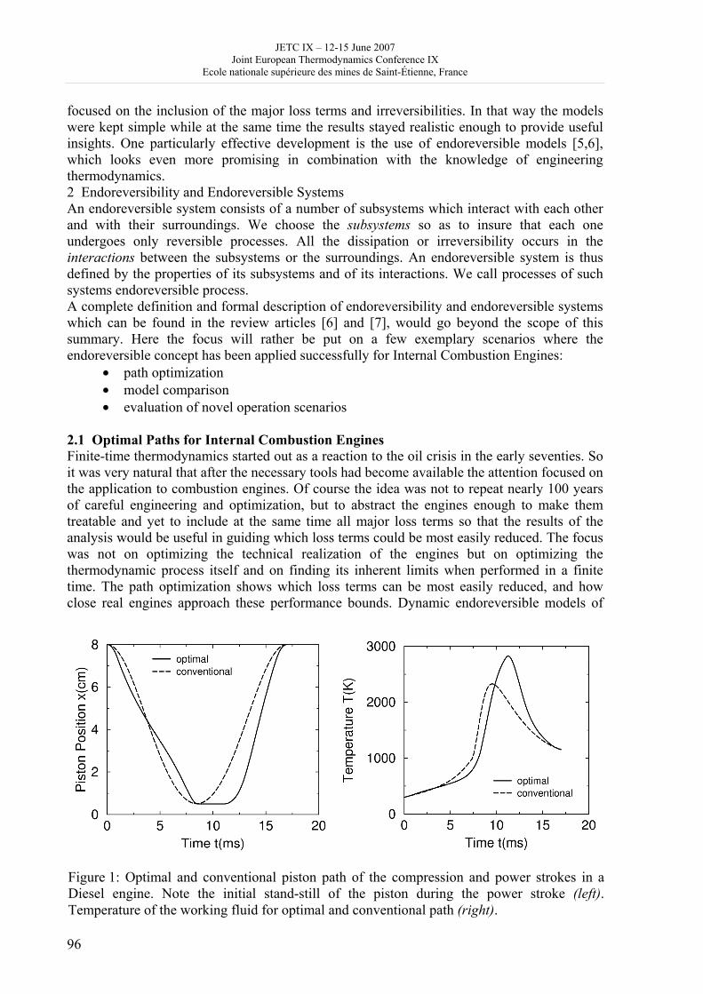
JETC IX – 12-15 June 2007 Joint European Thermodynamics Conference IX
Ecole nationale supérieure des mines de Saint-Étienne, France
96
focused on the inclusion of the major loss terms and irreversibilities. In that way the models were kept simple while at the same time the results stayed realistic enough to provide useful insights. One particularly effective development is the use of endoreversible models [5,6], which looks even more promising in combination with the knowledge of engineering thermodynamics. 2 Endoreversibility and Endoreversible Systems An endoreversible system consists of a number of subsystems which interact with each other and with their surroundings. We choose the subsystems so as to insure that each one undergoes only reversible processes. All the dissipation or irreversibility occurs in the interactions between the subsystems or the surroundings. An endoreversible system is thus defined by the properties of its subsystems and of its interactions. We call processes of such systems endoreversible process. A complete definition and formal description of endoreversibility and endoreversible systems which can be found in the review articles [6] and [7], would go beyond the scope of this summary. Here the focus will rather be put on a few exemplary scenarios where the endoreversible concept has been applied successfully for Internal Combustion Engines:
• path optimization • model comparison • evaluation of novel operation scenarios
2.1 Optimal Paths for Internal Combustion Engines Finite-time thermodynamics started out as a reaction to the oil crisis in the early seventies. So it was very natural that after the necessary tools had become available the attention focused on the application to combustion engines. Of course the idea was not to repeat nearly 100 years of careful engineering and optimization, but to abstract the engines enough to make them treatable and yet to include at the same time all major loss terms so that the results of the analysis would be useful in guiding which loss terms could be most easily reduced. The focus was not on optimizing the technical realization of the engines but on optimizing the thermodynamic process itself and on finding its inherent limits when performed in a finite time. The path optimization shows which loss terms can be most easily reduced, and how close real engines approach these performance bounds. Dynamic endoreversible models of
Figure 1: Optimal and conventional piston path of the compression and power strokes in aDiesel engine. Note the initial stand-still of the piston during the power stroke (left). Temperature of the working fluid for optimal and conventional path (right).
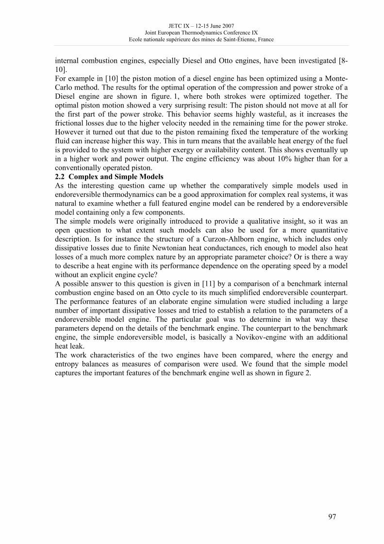
JETC IX – 12-15 June 2007 Joint European Thermodynamics Conference IX
Ecole nationale supérieure des mines de Saint-Étienne, France
97
internal combustion engines, especially Diesel and Otto engines, have been investigated [8-10]. For example in [10] the piston motion of a diesel engine has been optimized using a Monte-Carlo method. The results for the optimal operation of the compression and power stroke of a Diesel engine are shown in figure. 1, where both strokes were optimized together. The optimal piston motion showed a very surprising result: The piston should not move at all for the first part of the power stroke. This behavior seems highly wasteful, as it increases the frictional losses due to the higher velocity needed in the remaining time for the power stroke. However it turned out that due to the piston remaining fixed the temperature of the working fluid can increase higher this way. This in turn means that the available heat energy of the fuel is provided to the system with higher exergy or availability content. This shows eventually up in a higher work and power output. The engine efficiency was about 10% higher than for a conventionally operated piston. 2.2 Complex and Simple Models As the interesting question came up whether the comparatively simple models used in endoreversible thermodynamics can be a good approximation for complex real systems, it was natural to examine whether a full featured engine model can be rendered by a endoreversible model containing only a few components. The simple models were originally introduced to provide a qualitative insight, so it was an open question to what extent such models can also be used for a more quantitative description. Is for instance the structure of a Curzon-Ahlborn engine, which includes only dissipative losses due to finite Newtonian heat conductances, rich enough to model also heat losses of a much more complex nature by an appropriate parameter choice? Or is there a way to describe a heat engine with its performance dependence on the operating speed by a model without an explicit engine cycle? A possible answer to this question is given in [11] by a comparison of a benchmark internal combustion engine based on an Otto cycle to its much simplified endoreversible counterpart. The performance features of an elaborate engine simulation were studied including a large number of important dissipative losses and tried to establish a relation to the parameters of a endoreversible model engine. The particular goal was to determine in what way these parameters depend on the details of the benchmark engine. The counterpart to the benchmark engine, the simple endoreversible model, is basically a Novikov-engine with an additional heat leak. The work characteristics of the two engines have been compared, where the energy and entropy balances as measures of comparison were used. We found that the simple model captures the important features of the benchmark engine well as shown in figure 2.
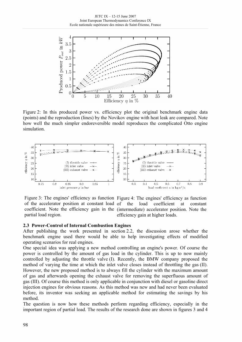
JETC IX – 12-15 June 2007 Joint European Thermodynamics Conference IX
Ecole nationale supérieure des mines de Saint-Étienne, France
98
Figure 2: In this produced power vs. efficiency plot the original benchmark engine data (points) and the reproduction (lines) by the Novikov engine with heat leak are compared. Note how well the much simpler endoreversible model reproduces the complicated Otto engine simulation.
2.3 Power-Control of Internal Combustion Engines After publishing the work presented in section 2.2, the discussion arose whether the benchmark engine used there would be able to help investigating effects of modified operating scenarios for real engines. One special idea was applying a new method controlling an engine's power. Of course the power is controlled by the amount of gas load in the cylinder. This is up to now mainly controlled by adjusting the throttle valve (I). Recently, the BMW company proposed the method of varying the time at which the inlet valve closes instead of throttling the gas (II). However, the new proposed method is to always fill the cylinder with the maximum amount of gas and afterwards opening the exhaust valve for removing the superfluous amount of gas (III). Of course this method is only applicable in conjunction with diesel or gasoline direct injection engines for obvious reasons. As this method was new and had never been evaluated before, its inventor was seeking an applicable method for estimating the savings by his method. The question is now how these methods perform regarding efficiency, especially in the important region of partial load. The results of the research done are shown in figures 3 and 4
Figure 3: The engines' efficiency as function of the accelerator position at constant load coefficient. Note the efficiency gain in the partial load region.
Figure 4: The engines' efficiency as function of the load coefficient at constant (intermediate) accelerator position. Note the efficiency gain at higher loads.
JETC IX – 12-15 June 2007 Joint European Thermodynamics Conference IX
Ecole nationale supérieure des mines de Saint-Étienne, France
99
while varying load and accelerator position. As only variant (I) really has a variable inlet pressure, in the other cases the valve timings are chosen to reproduce the first ones speed and power output. The surprising result was that the newer method was the best available. References [1] I. I. Novikov. The efficiency of atomic power stations. Journal Nuclear Energy II,
7:125-128, 1958. translated from Atomnaya Energiya, 3 (1957), 409. [2] F. L. Curzon and B. Ahlborn. Efficiency of a carnot engine at maximum power output.
Am. J. Phys., 43:22-24, 1975. [3] Adrian Bejan and J. L. Smith Jr. Thermodynamic optimization of mechanical supports
for cryogenic apparatus. Cryogenics, 14:158-163, 1974. [4] Bjarne Andresen, Peter Salamon, and R. Stephen Berry. Thermodynamics in finite
time: Extremals for imperfect heat engines. J. Chem. Phys., 66(4):1571-1577, 1977. [5] Morton H. Rubin. Optimal configuration of a class of irreversible heat engines. I. Phys.
Rev. A, 19(3):1272-1276, 1979. [6] K. H. Hoffmann, J. M. Burzler, and S. Schubert. Endoreversible thermodynamics. J.
Non-Equilib. Thermodyn., 22(4):311-355, 1997. [7] K. H. Hoffmann, J. Burzler, A. Fischer, M. Schaller, and S. Schubert. Optimal process
paths for endoreversible systems. J. Non-Equilib. Thermodyn., 28(3):233-268, 2003. [8] M. Mozurkewich and R. Stephen Berry. Optimal paths for thermodynamic systems:
The ideal otto cycle. J. Appl. Phys., 53(1):34-42, 1982. [9] Karl Heinz Hoffmann, Stanley J. Watowich, and R. Stephen Berry. Optimal paths for
thermodynamic systems: The ideal Diesel cycle. J. Appl. Phys., 58(6):2125-2134, 1985. [10] P. Blaudeck and K. H. Hoffmann. Optimization of the power output for the
compression and power stroke of the Diesel engine. In Y. A. Gögüs, A. Öztürk, and G. Tsatsaronis, Efficiency, Costs, Optimization and Environmental Impact of Energy Systems, volume 2 of Proceedings of the ECOS95 Conference, page 754, Istanbul, 1995. International Centre for Applied Thermodynamics (ICAT).
[11] A. Fischer and K. H. Hoffmann. Can a quantitative simulation of an Otto engine be accurately rendered by a simple Novikov model with heat leak? J. Non-Equilib. Thermodyn., 29(1):9-28, 2004.
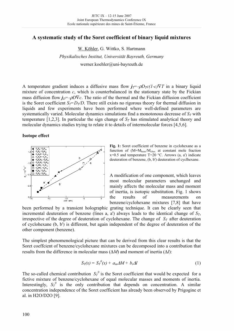
JETC IX – 12-15 June 2007 Joint European Thermodynamics Conference IX
Ecole nationale supérieure des mines de Saint-Étienne, France
100
A systematic study of the Soret coefficient of binary liquid mixtures
W. Köhler, G. Wittko, S. Hartmann
Physikalisches Institut, Universität Bayreuth, Germany
[email protected] A temperature gradient induces a diffusive mass flow jT=-ρDTc(1-c)∇T in a binary liquid mixture of concentration c, which is counterbalanced in the stationary state by the Fickian mass diffusion flow jD=-ρD∇c. The ratio of the thermal and the Fickian diffusion coefficient is the Soret coefficient ST=DT/D. There still exists no rigorous theory for thermal diffusion in liquids and few experiments have been performed where well-defined parameters are systematically varied. Molecular dynamics simulations find a monotonous decrease of ST with temperature [1,2,3]. In particular the sign change of ST has stimulated analytical theory and molecular dynamics studies trying to relate it to details of intermolecular forces [4,5,6]. Isotope effect
Fig. 1: Soret coefficient of benzene in cyclohexane as a function of (M=Mbenz/Mchex at constant mole fraction x=0.5 and temperature T=20 °C. Arrows (a, a') indicate deuteration of benzene, (b, b') deuteration of cyclhexane. A modification of one component, which leaves most molecular parameters unchanged and mainly affects the molecular mass and moment of inertia, is isotopic substitution. Fig. 1 shows the results of measurements on benzene/cyclohexane mixtures [7,8] that have
been performed by a transient holographic grating technique. It can be clearly seen that incremental deuteration of benzene (lines a, a') always leads to the identical change of ST, irrespective of the degree of deuteration of cyclohexane. The change of ST after deuteration of cyclohexane (b, b') is different, but again independent of the degree of deuteration of the other component (benzene). The simplest phenomenological picture that can be derived from this clear results is that the Soret coeffcient of benzene/cyclohexane mixtures can be decomposed into a contribution that results from the difference in molecular mass (ΔM) and moment of inertia (ΔI):
ST(x) = ST0(x) + amΔM + biΔI (1)
The so-called chemical contribution ST
0 is the Soret coefficient that would be expected for a fictive mixture of benzene/cyclohexane of equal molecular masses and moments of inertia. Interestingly, ST
0 is the only contribution that depends on concentration. A similar concentration independence of the Soret coefficient has already been observed by Prigogine et al. in H2O/D2O [9].
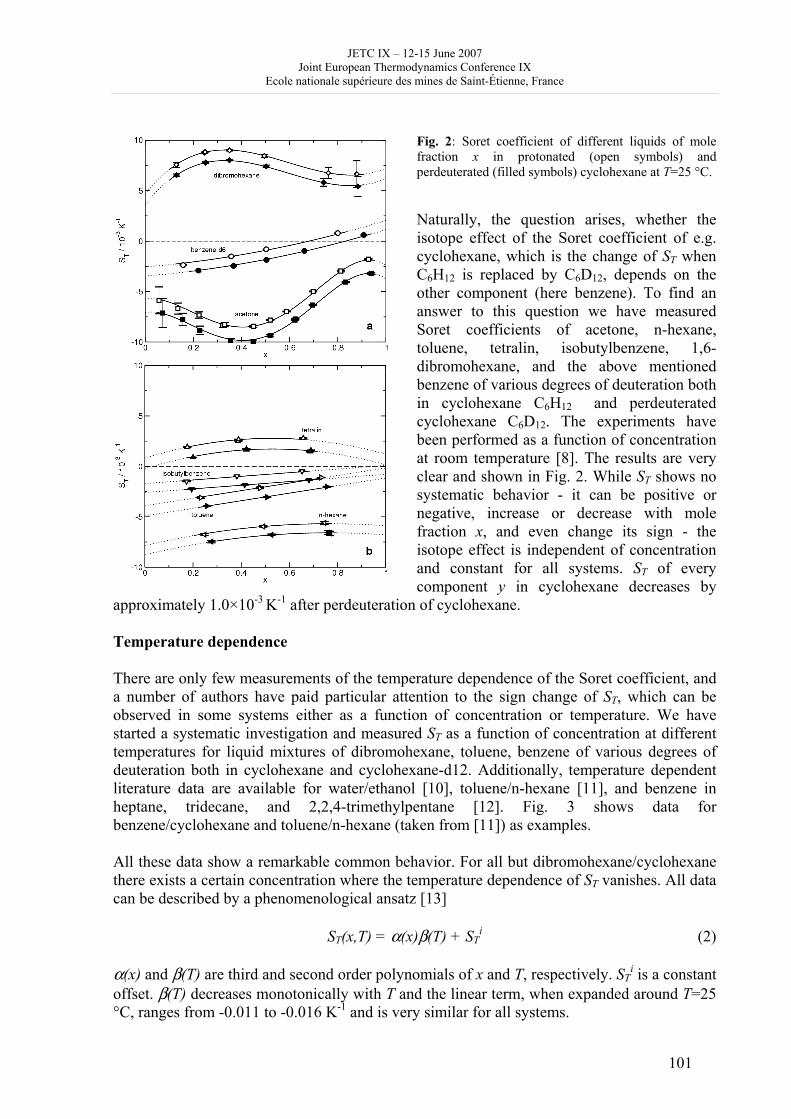
JETC IX – 12-15 June 2007 Joint European Thermodynamics Conference IX
Ecole nationale supérieure des mines de Saint-Étienne, France
101
Fig. 2: Soret coefficient of different liquids of mole fraction x in protonated (open symbols) and perdeuterated (filled symbols) cyclohexane at T=25 °C. Naturally, the question arises, whether the isotope effect of the Soret coefficient of e.g. cyclohexane, which is the change of ST when C6H12 is replaced by C6D12, depends on the other component (here benzene). To find an answer to this question we have measured Soret coefficients of acetone, n-hexane, toluene, tetralin, isobutylbenzene, 1,6-dibromohexane, and the above mentioned benzene of various degrees of deuteration both in cyclohexane C6H12 and perdeuterated cyclohexane C6D12. The experiments have been performed as a function of concentration at room temperature [8]. The results are very clear and shown in Fig. 2. While ST shows no systematic behavior - it can be positive or negative, increase or decrease with mole fraction x, and even change its sign - the isotope effect is independent of concentration and constant for all systems. ST of every component y in cyclohexane decreases by
approximately 1.0×10⁻³ K-1 after perdeuteration of cyclohexane. Temperature dependence There are only few measurements of the temperature dependence of the Soret coefficient, and a number of authors have paid particular attention to the sign change of ST, which can be observed in some systems either as a function of concentration or temperature. We have started a systematic investigation and measured ST as a function of concentration at different temperatures for liquid mixtures of dibromohexane, toluene, benzene of various degrees of deuteration both in cyclohexane and cyclohexane-d12. Additionally, temperature dependent literature data are available for water/ethanol [10], toluene/n-hexane [11], and benzene in heptane, tridecane, and 2,2,4-trimethylpentane [12]. Fig. 3 shows data for benzene/cyclohexane and toluene/n-hexane (taken from [11]) as examples. All these data show a remarkable common behavior. For all but dibromohexane/cyclohexane there exists a certain concentration where the temperature dependence of ST vanishes. All data can be described by a phenomenological ansatz [13]
ST(x,T) = α(x)β(T) + STi (2)
α(x) and β(T) are third and second order polynomials of x and T, respectively. ST
i is a constant offset. β(T) decreases monotonically with T and the linear term, when expanded around T=25 °C, ranges from -0.011 to -0.016 K-1 and is very similar for all systems.
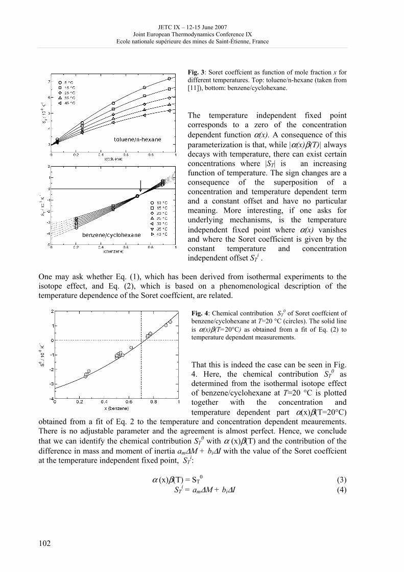
JETC IX – 12-15 June 2007 Joint European Thermodynamics Conference IX
Ecole nationale supérieure des mines de Saint-Étienne, France
102
Fig. 3: Soret coeffcient as function of mole fraction x for different temperatures. Top: toluene/n-hexane (taken from [11]), bottom: benzene/cyclohexane. The temperature independent fixed point corresponds to a zero of the concentration dependent function α(x). A consequence of this parameterization is that, while |α(x)β(T)| always decays with temperature, there can exist certain concentrations where |ST| is an increasing function of temperature. The sign changes are a consequence of the superposition of a concentration and temperature dependent term and a constant offset and have no particular meaning. More interesting, if one asks for underlying mechanisms, is the temperature independent fixed point where α(x) vanishes and where the Soret coefficient is given by the constant temperature and concentration independent offset ST
i . One may ask whether Eq. (1), which has been derived from isothermal experiments to the isotope effect, and Eq. (2), which is based on a phenomenological description of the temperature dependence of the Soret coeffcient, are related.
Fig. 4: Chemical contribution ST0 of Soret coeffcient of
benzene/cyclohexane at T=20 °C (circles). The solid line is α(x)β(T=20°C) as obtained from a fit of Eq. (2) to temperature dependent measurements. That this is indeed the case can be seen in Fig. 4. Here, the chemical contribution ST
0 as determined from the isothermal isotope effect of benzene/cyclohexane at T=20 °C is plotted together with the concentration and temperature dependent part α(x)β(T=20°C)
obtained from a fit of Eq. 2 to the temperature and concentration dependent meaurements. There is no adjustable parameter and the agreement is almost perfect. Hence, we conclude that we can identify the chemical contribution ST
0 with α (x)β(T) and the contribution of the difference in mass and moment of inertia amΔM + biΔI with the value of the Soret coeffcient at the temperature independent fixed point, ST
i:
α (x)β(T) = ST0 (3)
STi = amΔM + biΔI (4)
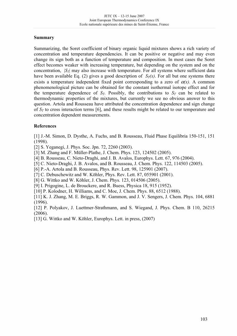
JETC IX – 12-15 June 2007 Joint European Thermodynamics Conference IX
Ecole nationale supérieure des mines de Saint-Étienne, France
103
Summary Summarizing, the Soret coefficient of binary organic liquid mixtures shows a rich variety of concentration and temperature dependencies. It can be positive or negative and may even change its sign both as a function of temperature and composition. In most cases the Soret effect becomes weaker with increasing temperature, but depending on the system and on the concentration, |ST| may also increase with temperature. For all systems where sufficient data have been available Eq. (2) gives a good description of ST(x). For all but one systems there exists a temperature independent fixed point corresponding to a zero of α(x). A common phenomenological picture can be obtained for the constant isothermal isotope effect and for the temperature dependence of ST. Possibly, the contributions to ST can be related to thermodynamic properties of the mixtures, but currently we see no obvious answer to this question. Artola and Rousseau have attributed the concentration dependence and sign change of ST to cross interaction terms [6], and these results might be related to our temperature and concentration dependent measurements. References [1] J.-M. Simon, D. Dysthe, A. Fuchs, and B. Rousseau, Fluid Phase Equilibria 150-151, 151 (1998). [2] S. Yeganegi, J. Phys. Soc. Jpn. 72, 2260 (2003). [3] M. Zhang and F. Müller-Plathe, J. Chem. Phys. 123, 124502 (2005). [4] B. Rousseau, C. Nieto-Draghi, and J. B. Avalos, Europhys. Lett. 67, 976 (2004). [5] C. Nieto-Draghi, J. B. Avalos, and B. Rousseau, J. Chem. Phys. 122, 114503 (2005). [6] P.-A. Artola and B. Rousseau, Phys. Rev. Lett. 98, 125901 (2007). [7] C. Debuschewitz and W. Köhler, Phys. Rev. Lett. 87, 055901 (2001). [8] G. Wittko and W. Köhler, J. Chem. Phys. 123, 014506 (2005). [9] I. Prigogine, L. de Brouckere, and R. Buess, Physica 18, 915 (1952). [10] P. Kolodner, H. Williams, and C. Moe, J. Chem. Phys. 88, 6512 (1988). [11] K. J. Zhang, M. E. Briggs, R. W. Gammon, and J. V. Sengers, J. Chem. Phys. 104, 6881 (1996). [12] P. Polyakov, J. Luettmer-Strathmann, and S. Wiegand, J. Phys. Chem. B 110, 26215 (2006). [13] G. Wittko and W. Köhler, Europhys. Lett. in press, (2007)
JETC IX – 12-15 June 2007 Joint European Thermodynamics Conference IX
Ecole nationale supérieure des mines de Saint-Étienne, France
104
Determination of solid-liquid-liquid equilibria in the ternary system Piperidine-sodium sulfate-water by Isoplethic Thermic Analysis: Study of
the isothermal sections 293K, 298K, 313K.
E. LABARTHE, N. KACIDEM, A.J. BOUGRINE,C. GOUTAUDIER, J.J COUNIOUX, H. DELALU
Laboratoire Hydrazines et Procédés-Université Claude Bernard Lyon 1-69622 VILLEURBANNE
[email protected] During the synthesis of N-aminopiperidine, we noted the formation of a salt of piperidinium. Then, we did a neutralization with soda. At this step, it occurs sodium sulfate which is at the origin of a separation of phase between an aqueous and an organic phase. However, sodium sulfate precipitates and prevents a complete demixting. That is why we started to study the ternary diagram Piperidine(PP)-Na2SO4-H2O in order to determine the optimal conditions for extraction of our useful product. Isoplethic Thermic Analysis (ATI) under isobar conditions, developed at the Hydrazines and Processes Laboratory, is a synthetic method of isothermal and isobar analysis well adapted to our study. Its principle is based on the measurement of the heating effects associated with the transformations of the system (appearance or disappearance of a phase) when its composition is modified. The mixture is maintained under quasi-isothermal conditions and the variations of temperature, about some hundredths of degree, are represented as function of the volume of water added to the system. Generally used for liquid-solid equilibrium, we also applied it for the establishment of the curves of demixion. Equilibria between condensed phases of this ternary diagram were studied at different temperatures:
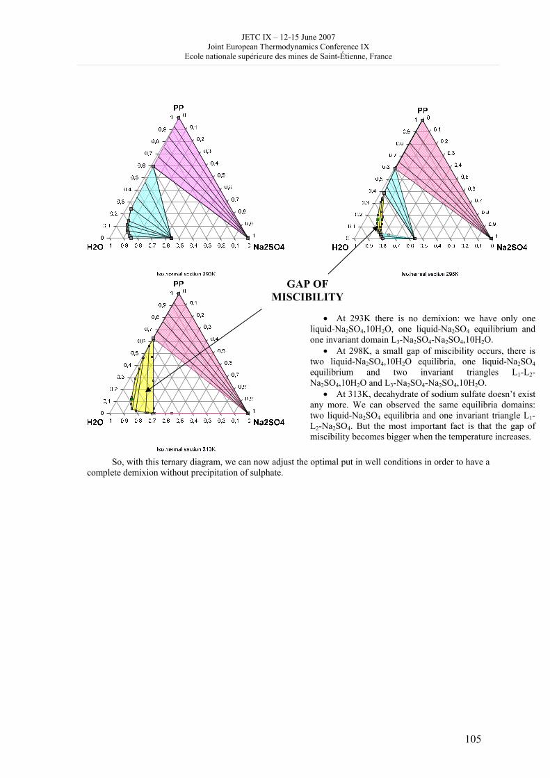
JETC IX – 12-15 June 2007 Joint European Thermodynamics Conference IX
Ecole nationale supérieure des mines de Saint-Étienne, France
105
So, with this ternary diagram, we can now adjust the optimal put in well conditions in order to have a
complete demixion without precipitation of sulphate.
L L
L
Na2SO4,10H2O Na2SO4,10H2O
GAP OF
MISCIBILITY
• At 293K there is no demixion: we have only one liquid-Na2SO4,10H2O, one liquid-Na2SO4 equilibrium and one invariant domain L3-Na2SO4-Na2SO4,10H2O.
• At 298K, a small gap of miscibility occurs, there is two liquid-Na2SO4,10H2O equilibria, one liquid-Na2SO4 equilibrium and two invariant triangles L1-L2-Na2SO4,10H2O and L3-Na2SO4-Na2SO4,10H2O.
• At 313K, decahydrate of sodium sulfate doesn’t exist any more. We can observed the same equilibria domains: two liquid-Na2SO4 equilibria and one invariant triangle L1-L2-Na2SO4. But the most important fact is that the gap of miscibility becomes bigger when the temperature increases.
JETC IX – 12-15 June 2007 Joint European Thermodynamics Conference IX
Ecole nationale supérieure des mines de Saint-Étienne, France
106
A "magmatic isotherm" for the exchange of Fe and Mg between an olivine solid solution and a melt
Morad Lakhssassi, Jacques Moutte and Bernard Guy
Ecole nationale supérieure des mines de Saint-Etienne, France
[email protected] The notion of isotherm was proposed to model chemical exchanges, in particular ion exchanges, between aqueous solutions and solid substrates. At thermodynamical equilibrium, for a given temperature and for one chemical component, the isotherm links the concentrations in the aqueous solution cf and in the solid substrate cs by an analytic law cf = f(cs). In the present work, we propose to extend this notion in the case of exchanges between solids and melts, under some validity conditions to be specified. We are interested in the chemical exchange between the mineral contained in a rock and presenting a solid solution, and a melt that flows across the pores of the rock. The example chosen is an olivine of variable composition between the Forsterite (Mg2SiO4) endmember and the Fayalite (Fe2SiO4) endmember and we aim to express chemical equilibrium within an isotherm cm = f(cs) where m indicates the melt and s the solid. In order to do so, we first write the equation for the exchange of one chemical component, for example the Forsterite, between the melt and the olivine : Mg2SiO4 (s) ⇔ Mg2SiO4 (m) At chemical equilibrium, the equality of chemical potentials in the melt and in the solid holds :
mFosFo ,, μμ = We will consider here ideal solutions both in solid and in magma; thus, the chemical potentials can be written : )ln(..2 ,
0,, sFosFosFo XRT+= μμ and )ln(..2 ,
0,, mFomFomFo XRT+= μμ
when the activity is equal to the molar fraction squared for stoechimetric reasons. By expressing the mass per volume concentrations cm et cs as functions of the molar fractions Xs et Xm, we get the searched law between cm et cs which is written for example for the Forsterite :
( )( ) 4,3
2,2
2,1
,, ...
)(βββ
β++
==sFosFo
sFosFomFo cc
ccfc (in kg/m3)
JETC IX – 12-15 June 2007 Joint European Thermodynamics Conference IX
Ecole nationale supérieure des mines de Saint-Étienne, France
107
when the iβ are constants depending on the following parameters : 0,sFoμ , 0
,mFoμ , 0,sFaμ , 0
,mFaμ ,
FoM , mFoV , , mFaV , , msolventV , , sFoV , and sFaV , where the iV are the molar volumes (in m3/mol) and FoM the molar mass (Kg/mol). In order to be able to write such a relation, we need to know the values of the different parameters involved (see Ghiorso et al. 2002) and to assume that the µ0 in the melt do not depend on the composition of this latter. In the case of a non ideal solution in the melt, the coefficients of the µ0 and of the solution model may be variable upon the composition of the melt. When compared with the isotherm written for an exchange with an aqueous solution, a hidden and important difference lies in what we can call the “magmatic solvent”, which we can compare to water in the case of the aqueous solution; XH2O is considered to be almost constant and close to 1, whereas in the case of basaltic melts for instance, the parameter Xsolvent of the fraction of the melt which is not the melted olivine can correspond to a fairly important quantity of SiO2, Al2O3, CaO, K2O etc , and can vary within a certain interval according to the olivine composition. The isotherm gives the possibility to predict the compositions we can observe in a system where a pervading melt reacts with a rock. Depending on the respective positions of the melt and of the rock on the isotherm, various behaviours are expected : appearance of discontinuities and propagation of transformation fronts, or propagation of “détente” waves.
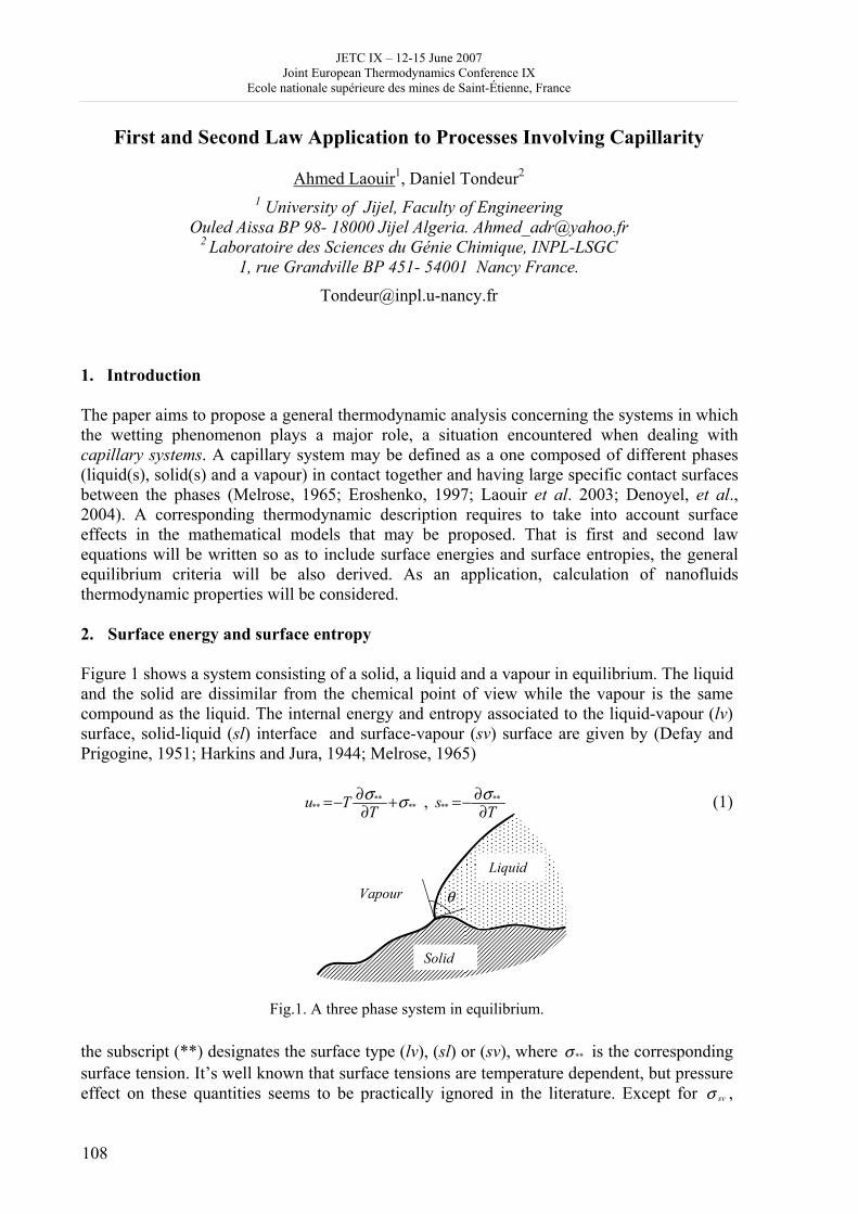
JETC IX – 12-15 June 2007 Joint European Thermodynamics Conference IX
Ecole nationale supérieure des mines de Saint-Étienne, France
108
First and Second Law Application to Processes Involving Capillarity
Ahmed Laouir1, Daniel Tondeur2
1 University of Jijel, Faculty of Engineering Ouled Aissa BP 98- 18000 Jijel Algeria. [email protected]
2 Laboratoire des Sciences du Génie Chimique, INPL-LSGC 1, rue Grandville BP 451- 54001 Nancy France.
[email protected] 1. Introduction The paper aims to propose a general thermodynamic analysis concerning the systems in which the wetting phenomenon plays a major role, a situation encountered when dealing with capillary systems. A capillary system may be defined as a one composed of different phases (liquid(s), solid(s) and a vapour) in contact together and having large specific contact surfaces between the phases (Melrose, 1965; Eroshenko, 1997; Laouir et al. 2003; Denoyel, et al., 2004). A corresponding thermodynamic description requires to take into account surface effects in the mathematical models that may be proposed. That is first and second law equations will be written so as to include surface energies and surface entropies, the general equilibrium criteria will be also derived. As an application, calculation of nanofluids thermodynamic properties will be considered. 2. Surface energy and surface entropy Figure 1 shows a system consisting of a solid, a liquid and a vapour in equilibrium. The liquid and the solid are dissimilar from the chemical point of view while the vapour is the same compound as the liquid. The internal energy and entropy associated to the liquid-vapour (lv) surface, solid-liquid (sl) interface and surface-vapour (sv) surface are given by (Defay and Prigogine, 1951; Harkins and Jura, 1944; Melrose, 1965)
****
** TTu σσ +∂∂−= , Ts **
** ∂∂−= σ (1)
Fig.1. A three phase system in equilibrium. the subscript (**) designates the surface type (lv), (sl) or (sv), where **σ is the corresponding surface tension. It’s well known that surface tensions are temperature dependent, but pressure effect on these quantities seems to be practically ignored in the literature. Except for svσ ,
Liquid
Solid
θVapour
JETC IX – 12-15 June 2007 Joint European Thermodynamics Conference IX
Ecole nationale supérieure des mines de Saint-Étienne, France
109
experimental data concerning temperature dependencies of surface tensions are scare. Using Young equation θσσσ coslvsvsl −= , slu and sls may be expressed as,
svlvlv
sl ucosT)cos(Tu +−
∂∂= θσθσ ; sv
lvsl sT
)cos(s +∂∂= θσ (2)
The contact angleθ of the specified solid and liquid couple is a thermodynamic property which is, as surface tensions, temperature and pressure dependent. 3. Energy and entropy balance The thermodynamic properties associated to the system shown in figure 1 involve those of the solid, the liquid, the vapour and those related to the contact surfaces discussed above. So the overall internal energy Ug for all the system is,
lvlvsvsvslslvvllssg AuAuAuumumumU +++++= (3)
us ,ul, uv are the specific internal energies of the three phases and usl , usv , ulv the internal energies related to the surfaces given by Eq. (1). Similarly, the overall entropy Sg is,
lvlvsvsvslslvvllssg AsAsAssmsmsmS +++++= (4) The general form of the energy balance equation is ,
)eeh(mWQdt
)EEU(dpcg
pcg ∑ ++++=++
&&& (5)
Ug, Ec and Ep are the overall internal energy, kinetic energy and potential energy of the system, Q& the rate of heat transfer, W& the power transfer, hg, ec and ep are the specific overall enthalpy, kinetic and potential energies related to the flow stream m& . The overall enthalpy hg is to be defined in relation to the energies transferred with matter across the system boundary (Laouir and Tondeur, 2004). The entropy balance equation is,
ε&&&
++= ∑ gg sm
TQ
dt)S(d (6)
where Sg is the overall entropy of the system, sg is the specific overall entropy of the corresponding flow stream and ε& the entropy production rate which is zero for reversible processes. 4. Equilibrium criteria The general equilibrium criteria may be derived by considering an infinitesimal change of state in the vicinity of the equilibrium point of a closed and non-moving system,
WQdEdU pg δδ +=+ and δεδ +=TQdS g (7)
JETC IX – 12-15 June 2007 Joint European Thermodynamics Conference IX
Ecole nationale supérieure des mines de Saint-Étienne, France
110
In many cases the work Wδ is zero (capillary rise, sessile drop…), in others it corresponds to the work of change in volume PdV− (bubble in a liquid, equilibrium of non-wetting liquid in a porous solid…). It should be stressed that pressure in capillary systems may not be uniform; the work is defined in relation to the pressure acting at the system boundary. The equilibrium state corresponds to the point at which entropy production ε is a maximum that is 0=δε . This is equivalent to say ε− is minimum, 0=−δε or 0=− δεT , the later leads to,
0=−++ gpg TdSdEPdVdU (8) an equation that gives the minimum of the differentiated quantity. For an equilibrium achieved at constant T and V, 0=+ pg dEdF and pg EF + is minimum ( ggg TSUF −= is the overall free energy of the system). If the equilibrium concerns an adiabatic system,
0==δεgdS , gS is maximum; assuming a constant volume, 0=+ pg dEdU and pg EU + constant in this case. 5. Thermodynamic properties of nanofluids Liquids containing suspended solid nanoparticles are termed nanofluids, the presence of the particles enhances dramatically the transport properties of the mixture (Boualit and Zeraibi, 2006; Trisaksri and Wongwises, 2007). Thermodynamic properties of such a fluid may be calculated as follows. The specific volume is lsg v)x(xvv −+= 1 where x is particles mass fraction, ls vv and solid and liquid specific volumes. According to Eq. (3) internal energy is
slslllssg AuumumU ++= , the particles are supposed spherical having a surface 24 rπ and a mass sv/.r/ 134 3π , therefore the specific wetted surface ssllsslsl m/xA)mm/(Aa =+= may be
expressed as r/xva ssl 13= . Specific internal energy of the fluid is slsllsg uau)x(xuu +−+= 1 and specific entropy is slsllsg sas)x(xss +−+= 1 ,
σσσ uu~T
Tr
xvu)x(xuu slsl
slsg +=⎥⎦⎤
⎢⎣
⎡ +∂
∂−+−+= 131 (9)
σσ ss~Tr
xvs)x(xss slslsg +=⎥⎦
⎤⎢⎣
⎡∂
∂−+−+= 131 (10)
specific enthalpy expression is ggg Pvuh += and the heat capacity defined by T/uc gg ∂∂= so,
σσ cc~T
Tr
xvc)x(xcc slslsg +=⎥
⎦
⎤⎢⎣
⎡
∂∂−+−+= 2
2131 (11)
sc and lc are the solid and liquid specific heats; c~s~u~ and , the average quantities of an
“ideal” blend for which there is no surface effects; σσσ csu and , are the quantities related to the wetting phenomenon which may be regarded as excess quantities. If )T(slsl σσ = is linear
σu and σs will be constant and σc zero, so the fluid will behave like an ideal blend. Using young equation, and knowing that )T(lvσ is practically linear for pure substances ( 022 ≈∂∂ T/lvσ ),
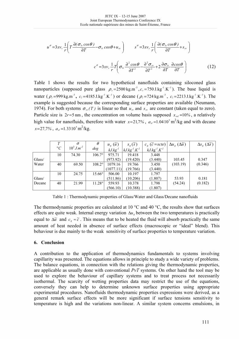
JETC IX – 12-15 June 2007 Joint European Thermodynamics Conference IX
Ecole nationale supérieure des mines de Saint-Étienne, France
111
⎟⎟⎠
⎞⎜⎜⎝
⎛+−
∂∂= svlv
lvs ucos
T)cos(T
rxvu θσθσσ 13 ⎟⎟
⎠
⎞⎜⎜⎝
⎛+
∂∂= sv
lvs s
T)cos(
rxvs θσσ 13
⎟⎟⎠
⎞⎜⎜⎝
⎛∂
∂∂
∂+∂
∂−∂
∂=T
cosTTT
cosTr
xvc lvsvlvs
θσσθσσ 213 2
2
2
2
(12)
Table 1 shows the results for two hypothetical nanofluids containing siloconed glass nanoparticles (supposed pure glass -3kg.m 2500=sρ , -1-1 KJ.kg 750 .cs = ). The base liquid is water ( -3kg.m 999=lρ , -1-1 KJ.kg 4185 .cl = ) or decane ( -3kg.m 724=lρ , -1-1 KJ.kg 2213 .cl = ). The example is suggested because the corresponding surface properties are available (Neumann, 1974). For both systems )T(svσ is linear so that svsv su and are constant (taken equal to zero). Particle size is nm 52 =r , the concentration on volume basis supposed %xvol 10= , a relatively high value for nanofluids, therefore with water %,x 721= , 510 041.asl = m2/kg and with decane
%,x 727= , 510 331.asl = m2/kg.
T °C
σ 103 J.m-2
θ deg
)( u~ug
kJ.kg-1 )(s~sg
kJ.kg-1.K-1 )( sctec~cg =
kJ.kg-1.K-1 )( u~u g ΔΔ )( s~sg ΔΔ
10 74.30 106.7° 975.71 (973.92)
19.418 (19.420)
3.448 (3.440)
Glass/ Water 40 69.50 108.2° 1079.16
(1077.11)19.766
(19.766) 3.450
(3.440)
103.45
(103.19)
0.347
(0.346)
10 24.75 15.66° 506.00 (511.86)
10.197 (10.206)
1.797 (1.807)
Glass/ Decane 40 21.99 11.28° 559.93
(566.10)10.378
(10.388) 1.798
(1.807)
53.93
(54.24)
0.181
(0.182)
Table 1 : Thermodynamic properties of Glass/Water and Glass/Decane nanofluids
The thermodynamic properties are calculated at 10 °C and 40 °C, the results show that surfaces effects are quite weak. Internal energy variation guΔ between the two temperatures is practically equal to u~Δ and c~cg ≈ . This means that to be heated the fluid will absorb practically the same amount of heat needed in absence of surface effects (macroscopic or “ideal” blend). This behaviour is due mainly to the weak sensitivity of surface properties to temperature variation. 6. Conclusion A contribution to the application of thermodynamics fundamentals to systems involving capillarity was presented. The equations allows in principle to study a wide variety of problems. The balance equations, in connection with the relations giving the thermodynamic properties, are applicable as usually done with conventional PvT systems. On other hand the tool may be used to explore the behaviour of capillary systems and to treat process not necessarily isothermal. The scarcity of wetting properties data may restrict the use of the equations, conversely they can help to determine unknown surface properties using appropriate experimental procedures. Nanofluids thermodynamic properties expressions were derived, as a general remark surface effects will be more significant if surface tensions sensitivity to temperature is high and the variations non-linear. A similar system concerns emulsions, in
JETC IX – 12-15 June 2007 Joint European Thermodynamics Conference IX
Ecole nationale supérieure des mines de Saint-Étienne, France
112
place of solid particles base liquid contains immiscible liquid droplets, the two liquids having a specified liquid-liquid surface tension )T(llσ . In this case contact surface lla may vary during a process as a result of droplets division or coalescence. References Boualit, H. Zeraibi, N. (2006). Numerical investigation of a laminar forced convection flow of nanofluids
in a uniformly heated tube. Int. conf. on micro and nano technologies, ICMNT’06, TiziOuzou, Algeria. Defay, R. Prigogine, I. (1951). Tension superficielle et adsorption, Dunod. Denoyel, R. Beurroies, I. Lefevre, B. (2004). Thermodynamics of wetting: information brought by microcalorimetry. Journal of Petroleum Science and Engineering, 45, pp 203 212. Eroshenko, V. (1997). Dimensionnalité de l’espace comme potentiel thermodynamique d'un système. Entropie, 202/203, pp 110 114. Harkins, W.D. Jura, G. (1944). An absolute method for the determination of the area of a finely divided crystalline solid. J. Am. Chem. Soc., 66, pp 1362-1373 Laouir,A. Tondeur,D.(2004). Bilans d’énergie et d’entropie étendues aux interactions interfaciales. Conférence internationale de mécanique avancée, CIMA’04, Boumerdès, Algérie. Laouir,A. Luo,L. Tondeur, D. Cachot,T. LeGoff,P.(2003). Thermal machines based on surface energy of
wetting. thermodynamic analysis. AIChE Journal, 49, pp 764-772. Melrose,J.C. (1965). On the thermodynamic relations between immersional and adhesional wetting. Journal of
colloid science, 20, pp 801 821. Neumann, A.W. (1974). Contact angles and their temperature dependence. Advances in colloid and interface science. 4, pp. 105-191. Triaksri, V. Wongwises, S. (2007). Critical review of heat transfer characteristics of nanofluids. Renewable and Sustainable Energy Reviews. 11, pp 512-523.
JETC IX – 12-15 June 2007 Joint European Thermodynamics Conference IX
Ecole nationale supérieure des mines de Saint-Étienne, France
113
Teaching and Learning Thermodynamics at school
Le Marechal Jean-François, El Bilani Rania
UMR I.C.A.R., INRP, CNRS, Université de Lyon, France
[email protected], [email protected] Teaching thermodynamics begins in primary school, with the first notion of temperature, and continues up to university. Many teaching and learning difficulties have been observed at all levels (Goedhart & Kaper, 2002). Typical examples at the earliest school levels cover changes of state and the difficult differentiation of the concepts of heat, energy and temperature. The problem of attributing a substantive character to heat has also been observed (Watson et al. 1997). Further along, at the university level, giving meaning to the difference between free energy, enthalpy and Gibbs energy is not easy, nor is the introduction of entropy. At such a level, introducing thermodynamics concepts relies primarily on the use of mathematics, for example partial derivatives, which is not possible at school level. How can teaching thermodynamics occur at lower levels? Energy is a unifying concept in physics and its teaching can no longer be viewed as a notion that looks different, to learners, in mechanics, electricity, chemistry, biology, etc. For example, incoherence occurs when learners are told that breaking a chemical bond costs energy in chemistry courses, whereas high-energy bonds store energy in ATP when biology is concerned (Boo & Watson, 2001). Moreover, it is probably not the best way for learners to make meaning out of the energy concept by reducing it to the use of formulas that are specific to each field, such as ½ m.v2, R.i2.t, m.C.��, and so on. One unified way to teach energy at school has been to present it as a variable with the following properties: energy is conservative, can be stored, transformed, and transferred (Gaidioz et al. 1998). Energy transfer can be done between two systems by one of the three modes: work, heat or rays. Such a general and unified introduction has proved to be teachable at secondary school level and usable in the many different fields that rely on energy, such as chemistry. Energy is much used in chemistry, and we introduced it at the upper secondary school level with a teaching sequence that considers three different aspects: a social aspect with the use of energy in heating and transport, aiming at giving students scientific literacy; a laboratory aspect as a tool to understand change of state or exothermic reactions; and a fundamental aspect with its interest in better understanding chemical bonds and their strengths. The teaching sequence was designed and then evaluated. It involved laboratory work and simulations. Although students’ difficulties to transfer our general and unified introduction of energy to the specific cases considered in chemistry studies still appeared, pre- and post-test showed an improvement of the basic conceptions on thermodynamics. We could also understand how the experimental and computer tasks had a positive impact on learning. BOO H.-K. & WATSON J. R. (2001). Progression in High School Students’ (Aged 16-18). Conceptualizations
about Chemical Reactions in Solution. Science Education, 85, pp. 568–585. GAIDIOZ P., MONNERET A. & TIBERGHIEN A. (1998). Introduction à l'énergie. Collection : Appliquer le
programme. Lyon: CRDP de Lyon. GOEDHART M. J. & KAPER W. (2002). From Chemical Energetics to Chemical Thermodynamics. In J. K.
Gilbert et al. (eds). Chemical Education: Towards Research-Based Practice, pp. 339-362. WATSON J. R., PRIETO T. & DILLON J. S. (1997). Consistency of Students’ Explanations about Combustion. Science Education, 81, pp. 425–444.
JETC IX – 12-15 June 2007 Joint European Thermodynamics Conference IX
Ecole nationale supérieure des mines de Saint-Étienne, France
114
Pattern formation in convective instabilities in a colloïdal suspension
Stefano Mazzoni, F. Giavazzi, R. Cerbino, M. Giglio and A. Vailati
European Space Agency - ESTEC HME-GAP, Keplerlaan 1, 2201AZ, Noordwijk ZH, The Netherlands
[email protected] Convection is a ubiquitous process in nature. The transport of heat inside stars and planets, the atmospheric circulation as well as the formation of deep currents in oceans are just a few examples of natural phenomena that are driven by convection. Traditionally, convective phenomena implicitly refer to heat transport by means of the macroscopic motion of the fluid itself, due to the fact that the vast majority of natural convective systems are of thermal nature. The earliest controlled observations of thermal convection are recognized to be the experiments of Bénard (1900), while, on the theoretical side, the fundamental work is that of Lord Rayleigh (1920). As a tribute, thermal convection is often referred as Rayleigh-Bénard instability. Despite the fact that the foundation of theory of convection as we now understand it dates back to nearly one century ago, convective phenomena are still of interest among the scientific community either from a theoretical or experimental point of view. Besides interesting technological problems (for instance the efficiency of cooling of electronic equipment), convection is worth studying due to diverse realms of scientific relevance it is related with. Let us discuss a few of them that are of interest in the present work. Although many studies of convective heat transport exist, the basic properties of heat transfer at high Rayleigh number (the Rayleigh number (Ra) is a dimensionless number that expresses the stress applied to the fluid) are still unclear. It is believed that the overall heat transferred by the convecting fluid should obey a power law scaling relation as a function of Ra, but no definite answer still exists about the value of the exponent of such a power law. This problem is of great interest since often convective regimes of natural system are high Rayleigh ones, and our present understanding of many of them would benefit from a detailed description of the heat transport properties. Another interesting facet of convection is the formation of spatiotemporal patterns. As often observed in far from thermal equilibrium systems, the non-equilibrium condition is a source of order at a macroscopic lengthscale. In the specific case of convective instabilities, the motions of the fluid are organized in a vast range of patterns whose features depend on the convective regime (expressed by Ra) and on the properties of the fluid. Convection is an ideal tool to study the problem of pattern formation outside of equilibrium, since laboratory based, controlled experiments are relatively easy to perform. Convective patterns are easy to generate and can be visualized by means of simple optical techniques, based on the principle that the hot and cold flows of fluid alter the wavefront of a light beam that impinges onto the sample. Finally, convection can be considered a prototypic system for the study of the transition to turbulence and chaotic behaviour. When increasing Ra, the spatial patterns, from the ordered state that characterize convection at low regimes, undergo a progressive transition to spatiotemporal disorder via the formation of spatial defects and time dependences, that eventually lead to fully developed turbulence. In this work we will focus our attention on a peculiar kind of convective instability, characterized by high values of the Rayleigh number Ra and of the Prandtl number Pr. The latter is a dimensionless number that expresses the ratio
JETC IX – 12-15 June 2007 Joint European Thermodynamics Conference IX
Ecole nationale supérieure des mines de Saint-Étienne, France
115
of viscosity over thermal diffusivity (and is therefore completely determined by the fluid properties). The peculiarity of such a convective regime relies on the fact that even if the convective regime is vigorous, the high value of Pr influences the flow in a way that it enhances its laminarity. In this way, ordered patterns are observed even if the convective regime is high. The study of high Prandtl convection is of interest in the particular problem of mantle convection, where the viscosity of the convective sample (that is rock) is nearly infinite (mantle convection is often referred as infinite Prandtl convection). However, the execution of an experimental investigation of high Ra, Pr convection is rather difficult, since these two conditions are in general difficult to meet simultaneously. This problem can be circumvented by considering solutal convection. We here present an experimental study of convective instabilities where the quantity that is convected by the fluid is the concentration of colloidal particles instead of heat as in usual Rayleigh-Bénard instability. This allows us to exploit the peculiar features of macromolecular suspensions to reach high (solutal equivalent of) Ra and Pr flows. The results here presented can be discussed within the framework of traditional thermal convection due to the existence of a formal analogy between the two cases. We will discuss the existence of a scaling relation for the mass transport during the onset of convection, obtaining an exponent comparable with those reported for turbulent thermal convection. Moreover, a topological analysis of the pattern will be presented, outlining a parallel between the observed cellular pattern (often called spoke pattern) and a peculiar kind of planar tessellation called Voronoi diagram. We will finally exploit this parallel in trying to characterize the progressive transition to spatial disorder when increasing the convective regime.
JETC IX – 12-15 June 2007 Joint European Thermodynamics Conference IX
Ecole nationale supérieure des mines de Saint-Étienne, France
116
Hyperbolic Reaction-Diffusion model for virus infections
Vicenç Méndez and José Casas-Vázquez
Grup de Física Estadística. Departament de Física. Universitat Autònoma de Barcelona. E-08193 Bellaterra (Cerdanyola) Spain.
[email protected], [email protected] Abstract We propose a reaction-diffusion model to study the front propagation of viruses growing in a bacterial colony. From a mesoscopic description we consider that viruses spread according to non-Markovian random walks obtaining a set of hyperbolic reaction-diffusion equations of three components. There is an excellent agreement between our predictions and experimental results. However, this agreement does not exist when random walks are Markovian and the resulting reaction-diffusion equations are of parabolic type. 1. Introduction
Reaction-diffusion equations have been studied extensively as mathematical models of systems with reactions and diffusion across a wide of applications. Most studies consider that the transport process is described by the Fick’s law. The resulting parabolic reaction-diffusion equation (Fisher equation) admits travelling wave solutions propagating with a constant speed which grows unboundedly with the reaction rate. More recently, it has been shown [1] that Fisher equation always overestimates the value of the front speed in neglecting the waiting time between jumps in comparison with the characteristic evolution time. However, in many process of biological interest both characteristic times may be of the same order, i.e. cannot be neglected. The first-order correction converts the reaction-diffusion equation into one of hyperbolic type. This equation predicts fronts propagating with constant speed exhibiting an upper bound in the fast reaction limit. In some ecological applications we have shown that the front speed of hyperbolic reaction-diffusion equations (HRD) is in a better agreement with the observed data than that obtained from the Fisher equation [2]. In this work we investigate the spreading dynamics of viruses which infect host bacteria. The process we want to model consists in the virus-bacteria interaction and the virus dispersal within the bacterial colony. We derive from a mesoscopic level a hyperbolic reaction-diffusion equation for the virus concentration. We also show that parabolic equations are inadequate as they do not take into account the time elapsed between the adsorption of a virus to a bacterium and the release of newborn viruses to the medium. This time will be estimated to be of the order of 20 min which is not negligible in front of the evolution time that is of about some hours. It is well known from virology that the virus reproduction within host bacteria causes the death of the bacteria and it is observed experimentally that the invaded area (plaque) can be regarded as a propagating front with constant speed [3]. The plaque is formed due to the adsorption of viruses to host bacteria, their replication within and the spread of the new generation after lysis. We deal, in particular, with virus phages such as T7 for which plaques grow unboundedly in a medium containing agar-immobilized stationary-phase host bacteria. Our model consists in three species: viruses (V), host bacteria (B) and infected bacteria (I). Their interactions (lytic cycle) can be summarized as follows:
JETC IX – 12-15 June 2007 Joint European Thermodynamics Conference IX
Ecole nationale supérieure des mines de Saint-Étienne, France
117
1 2k kV B I Y V+ ⎯⎯→ ⎯⎯→ ⋅ (1) where Y is the number of new viruses released per virus particle (yield), 1k is the rate of adsorption of viruses to a host bacteria and 2k is the death rate of infected bacteria.
2. Mesoscopic and macroscopic equations
2.1. Kinetic equations In order to deduce the interaction term between the three species, let us consider a homogeneous medium composed initially of infected bacteria and a few free viruses. The adsorption process can be described by the equation
1ddV k VBt
= − (2)
As for each adsorbed bacteria one viruses is “removed” one has d / d d / dV t B t= which can be integrated to yield B V C= + , where C is an integration constant. Integrating Eq. (1) one gets the equation
01
0
( ) ln ln V CV Cg V Ck tV V
⎛ ⎞++⎛ ⎞≡ − =⎜ ⎟⎜ ⎟⎝ ⎠ ⎝ ⎠
(3)
where 0 0C B V= − , 0 ( 0)B B t= = and 0 ( 0)V V t= = . For the virus replication we consider the logistic growth equation
2max
d 1dV Vk Vt V
⎛ ⎞= −⎜ ⎟
⎝ ⎠. (4)
If adsorption takes place at 0t = and we define the delay time τ as the time elapsed from the adsorption and the replication of max / 2V viruses, its solution reads
( )21( )
max( ) 1 τ −− −= + k tV t V e . (5)
On the other hand, from the conservation of the number of viruses and infected bacteria one has max max( ) ( )V t YI t V YI+ = = which can be introduced into Eq. (4) to yield
2max
d d 1d dV I IY k YIt t I
⎛ ⎞= − = −⎜ ⎟
⎝ ⎠. (6)
Finally, the set of kinetic equation reads d / d ( , , )VV t F V B I= , d / d ( , , )BB t F V B I= , d / d ( , , )II t F V B I= where
1 2 1 1 2max max
1 , , 1⎛ ⎞ ⎛ ⎞
≡ − + − ≡ − ≡ − −⎜ ⎟ ⎜ ⎟⎝ ⎠ ⎝ ⎠
V B II IF k VB k YI F k VB F k VB k I
I I (7)
2.2. Dispersal equation In order to propose an equation for the virus dispersal in agar we start form the mesoscopic equation for the virus number at point x at time t obtained from the continuous-time random walk with reaction [4]
0 0( , ) ( ) ( ,0) d d ( , ) ( , ) d ( ) ( )φ Ψ φ′ ′ ′ ′ ′ ′ ′ ′ ′= + − − + −∫ ∫ ∫
t t
VV x t t V x t x x t V x x t t t t F t t (8),
where ( , )Ψ x t is the probability density function (PDF) of performing a jump of length x after waiting a time t and ( )tφ is the survival probability which can be written in the form
JETC IX – 12-15 June 2007 Joint European Thermodynamics Conference IX
Ecole nationale supérieure des mines de Saint-Étienne, France
118
0( ) 1 d ( )φ ϕ′ ′= − ∫
tt t t with ( )tϕ the waiting time PDF. Transforming (8) by Fourier–Laplace and dividing by ( )sϕ one has
1 1 1 1 1( , ) 1 ( , 0) ( ) ( , ) 1 ( , )( ) ( ) ( )
Φϕ ϕ ϕ
⎛ ⎞ ⎛ ⎞= − = + + −⎜ ⎟ ⎜ ⎟
⎝ ⎠ ⎝ ⎠VV k s V k t k V k s F k s
s s s s s (9)
where we have assumed that jump lengths and waiting times are decoupled random variables, i.e. ( , ) ( ) ( )Ψ Φ ϕ=k s k s . To be more explicit we take a Gaussian PDF of jumps
22 2( ) 1 2τΦ τ−= −D kk e D k in the diffusive limit and the non-Markovian waiting-time PDF 2 /( ) ( / ) τϕ τ −= tt t e , where τ stands for the characteristic waiting time between jumps. Note
that we have intentionally taken the same notation for this time as for the half reproduction time for viruses because this means that they reproduce when they are at the sedentary stage only. Introducing the above definitions into Eq. (9) and inverting by Fourier–Laplace we get
2 21 12 2τ τ∂ + ∂ = ∂ + + ∂t t x V t VV V D V F F , that is, the hyperbolic reaction-diffusion equation [5] for the viruses. As the diffusion of viruses is hindered by the presence of a suspension of spheroids (host bacteria) we must take also into account the Fricke’s equation
*(1 ) /(1 / )D f D f ς= − + , where 0 max/f B B= is the concentration of bacteria relative to its maximum possible value for a fixed nutrient concentration, ς is a parameter which takes care of the shape of bacteria and is equal to 1.67 for E. Coli, and *D is the diffusion coefficient for free viruses in agar.
3. Parameter estimation and results
The adsorption rate between T7 and E. Coli was estimated from fitting Eq. (3) to experimental data [6] as shown in Figure 1 (inset). As a result, we obtained 1 (1.29= ±k 90.59) 10−× ml/min. By fitting (5) to the one-step-growth curve for the replication of T7 within E. Coli [7] (main curve in Figure 1) we got 1
2 1.39min−=k , τ = 18.4 min and max 0/ 34.5Y V V= = . The diffusion coefficient of T7 in agar can be approximated to that of P22 because it is very similar to T7 in size and shape [8], * 8 24 10 cm /sD −= × . The set of evolution equations for the number of viruses, host bacteria and infected bacteria
2 2
2 2 , ( , , ), ( , , )2 2
VV B I
FV V V B ID F F V I B F V I Bt t x t t t
τ τ ∂∂ ∂ ∂ ∂ ∂+ = + + = =∂ ∂ ∂ ∂ ∂ ∂
,(10)
with the interaction terms defined as in (7), describes a propagating front invading the unstable state 0(0, ,0)B . The dimensionless front speed c (the front speed is calculated by multiplying c by 2Dk ) is calculated by computing the minimum value of c for any 0λ > from the characteristic equation [9]
( ) ( ){ }3 * 2 2 * 21 12 21 1 1 1λ τ λ τ κ⎡ ⎤− + − + +⎣ ⎦c c c
{ }*121 1 ( 1) ( 1) 0λ κ τ κ⎡ ⎤− + − − + − =⎣ ⎦c Y Y , (11),
where the dimensionless quantities are defined as *2kτ τ= and 1 2 max/( )k f k Bκ = . In Figure 2
we plot our results obtained from Eq. (11) for the two extreme values of 1k (solid and dashed lines) together with the parabolic case where 0τ = . Symbols represent the experimental results [3] for Bmax = 107 ml–1 (Fig. 1a) and Bmax = 108 ml–1 (Fig. 1b).
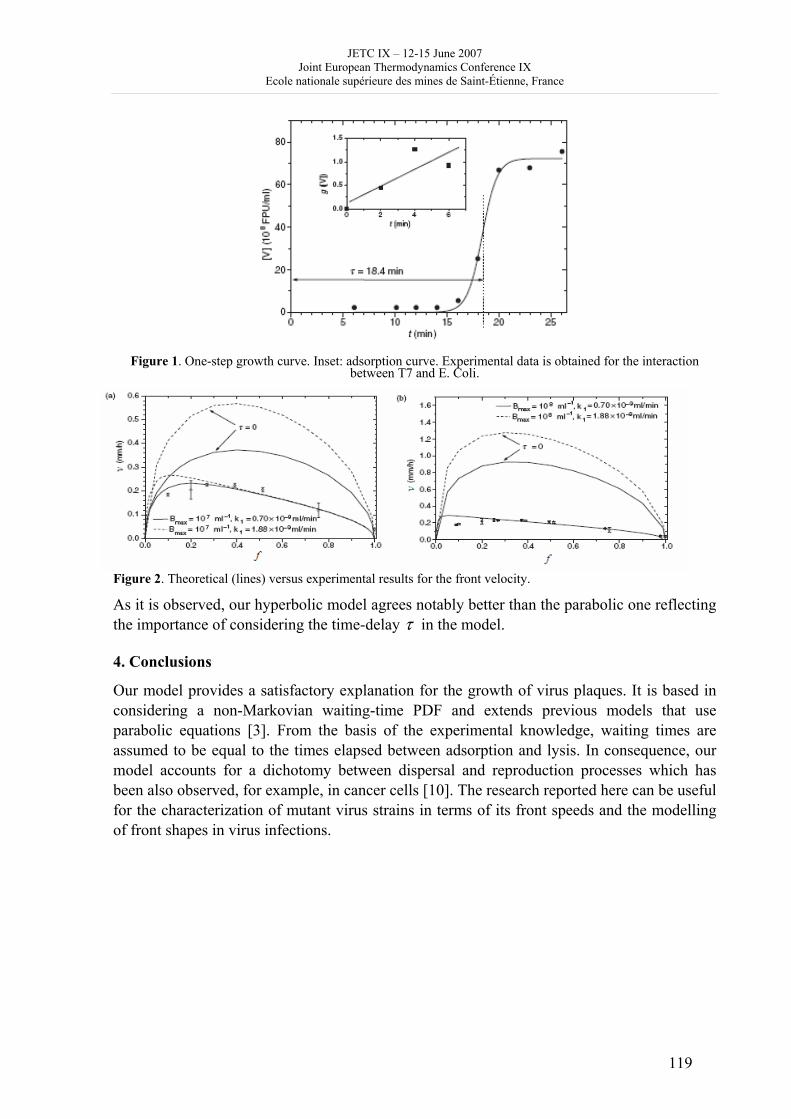
JETC IX – 12-15 June 2007 Joint European Thermodynamics Conference IX
Ecole nationale supérieure des mines de Saint-Étienne, France
119
Figure 1. One-step growth curve. Inset: adsorption curve. Experimental data is obtained for the interaction
between T7 and E. Coli.
Figure 2. Theoretical (lines) versus experimental results for the front velocity.
As it is observed, our hyperbolic model agrees notably better than the parabolic one reflecting the importance of considering the time-delay τ in the model. 4. Conclusions
Our model provides a satisfactory explanation for the growth of virus plaques. It is based in considering a non-Markovian waiting-time PDF and extends previous models that use parabolic equations [3]. From the basis of the experimental knowledge, waiting times are assumed to be equal to the times elapsed between adsorption and lysis. In consequence, our model accounts for a dichotomy between dispersal and reproduction processes which has been also observed, for example, in cancer cells [10]. The research reported here can be useful for the characterization of mutant virus strains in terms of its front speeds and the modelling of front shapes in virus infections.
JETC IX – 12-15 June 2007 Joint European Thermodynamics Conference IX
Ecole nationale supérieure des mines de Saint-Étienne, France
120
References [1] J. Fort and V. Méndez, Rep. Prog. Phys. 65 (2002) 895 [2] V. Ortega-Cejas, J. Fort and V. Méndez, Ecology 85 (2004) 258 [3] J. Yin and J. S. McCaskill, Biophys. J. 61 (1992) 1540 [4] S. Fedotov and V. Méndez, Phys. Rev. E 66 (2002) 030102 (R) [5] D. Jou, J. Casas-Vázquez and G. Lebon, Extended Irreversible Thermodynamics, (3rd ed., Springer, Berlin, 2001) [6] K. Shishido, A. Watarai, S. Naito and T. Ando, J. Antibiot. (Tokyo) 28 (1975) 676 [7] J. Yin, J. Bacteriol. 175 (1993) 1272 [8] H. W. Ackermann, Path. Biol. 24 (1976) 359 [9] J. Fort and V. Méndez, Phys. Rev. Lett. 89 (2002) 178101 [10] S. Fedotov and A. Iomin, Phys. Rev. Lett. 98 (2007) 118101
JETC IX – 12-15 June 2007 Joint European Thermodynamics Conference IX
Ecole nationale supérieure des mines de Saint-Étienne, France
121
Measurement of Soret coefficient in aqueous solutions.
Alexandr Mialdun, Valentina Shevrsova
MRC, Department of Chemical Physics, Université Libre de Bruxelles CP 165/62, av. F.D. Roosevelt 50, B–1050 Brussels, Belgium
[email protected] Introduction Transport coefficients in gases can be rather well estimated by kinetic theory but the situation is less favorable for liquid mixtures. Thermal diffusion in liquids is not so well understood even for binary mixtures. Soret effect is a thermodynamics quantity and its sign may depend on considered system and surrounding conditions. In some aqueous solutions the Soret coefficient may change sign depending on composition and temperature. The most advanced theoretical models are not complete for such systems and they should be more extensively verified by experimental measurements. Some of existing methods work well only for positive Soret coefficients. The most often used in the experiments binary mixture is water-ethyl alcohol. In the present experimental study the new experimental technique was validated against the literature data for water/ethanol mixture. The quantitative comparison for C0=0.51 and C0=0.61 reveals a good agreement with published data. Experimental Optical methods The proposed technique employs optical method of observation (interferometry). The main features of optical methods are non-intrusiveness and sensitivity. A significant advantage of these methods is the absence of mechanically driven parts in contact with liquid, so measurements do not disturb the experiment. The main disadvantage is that the media under investigation must be transparent. The measurement of thermal diffusion coefficients requires establishing a temperature gradient in the experimental cell. The absence of convection in the cell is crucial for achieving purely diffusive heat and mass transfer. It imposes an experimental constrains: heating from above and the working mixtures should have positive Soret effect. One of the traditional techniques is a beam deflection technique, where the evolution of composition is observed via deflection of a laser beam passing through the medium [1], [2]. Another important technique is the Thermal Diffusion Forced Rayleigh Scattering [3], where a grating created by the interference of two laser beams is converted into temperature grating by a chemically inert dye. Thus, the light is used to create a temperature gradient inside small zone of a liquid instead of differentially heated rigid walls. The refractive index grating read by a third laser beam. Recent advances in lasers and electronic cameras and increasing possibilities of computer-aided data processing have enabled considerable progress in the development of new optical measurement techniques. The present manuscript details the development of a new technique on the basis of optical digital interferometry to investigate the thermal diffusion process in liquids. The optical interferometer coupled with digital recording and processing is used for very accurate determination of refractive index variations. This method has several important advantages: allows measuring concentration and temperature distributions not only between hot and cold plates, but throughout the entire thermo/diffusion path. It allows to study transient regime of
JETC IX – 12-15 June 2007 Joint European Thermodynamics Conference IX
Ecole nationale supérieure des mines de Saint-Étienne, France
122
diffusion and Soret separation. Another important feature of the method is that it gives clear evidence of convective motion in the cell (if it presents). Experimental set_up The set-up was developed using the concept of Mach-Zehnder interferometer The light beam of constant frequency He-Ne laser (wavelength λ=632.8 nm) passes through the beam splitter where it splits into two beams of equal intensity. One of them (object beam) goes through the experimental cell perpendicular to the temperature gradient. Another one (reference beam) bypasses the cell. After passing mirrors the object and reference beams interfere with each other. The resulting interference fringes are captured by the CCD camera (1280 x 1024) pixels sensor. An optical cubic cell (Soret cell) of internal size L=10 mm is made of quartz. The top and bottom of the cell are made from copper and they are kept at different constant temperatures by Peltier modules (heating from above). The spatial temperature variation in the cell induces mass transfer through the Soret effect. Both temperature and composition variations contribute to the spatial distribution of the refractive index that modulates the wave-front of the optical beam. Each interferogram is reconstructed by performing a 2D fast Fourier transform (FFT) of the fringe image, filtering a selected band of the spectrum, performing an inverse 2D FFT of the filtered result and phase unwrapping. Knowledge of phase shifts gives information about the local gradients of composition inside of the fluid both for steady state and dynamic regimes. Composition analysis After fringe analysis one gets a spatial distribution of the total phase shift in the object beam caused by the optical properties of the liquid. Assume that the initial refractive index of the homogeneous mixture is n0(T0,C0), after a short period of time the refractive index changes to n(x,z,t) at the point (x,z) for some reasons (temperature and concentration variation). The change of the refractive index Δn may be obtained from the unwrapped phase change Δ φ using the expression:
ϕπλ Δ=−=Δ
Lnyxnn
2),( 0
where λ is the wavelength and L is the thickness of the liquid in the direction of the optical pathway. For the given wavelength, the variation of the refractive index includes temperature and concentration contributions
)1(),,(),,(),,(0000 ,,
tyxCCntyxT
Tntyxn
CTCT
Δ⎟⎠⎞
⎜⎝⎛
∂∂+Δ⎟
⎠⎞
⎜⎝⎛
∂∂=Δ
Because several very different time scales are involved in the process, the Eq.1 can be decomposed. The temperature dependent component of the refractive index will saturate relatively fast: first term in Eq.1 is considered while Δ C=0. And later in time the refractive index will change only due to the Soret induced variations of concentration field (the first term is a constant). Results A set of experiments was done with water-ethanol mixtures belonging to the region with positive Soret coefficient, namely for water mass fractions C0=0.49, 0.613. No hydrodynamic instabilities are expected for these mixtures. The mean temperature in these experiments was kept at ~297.5K and ΔT=10K. One of the close mixtures, C0=0.6088, was used for the kind of experimental benchmark, see ref. [4]. To avoid bubble in the long duration experiments the mixtures were degassed. Due to
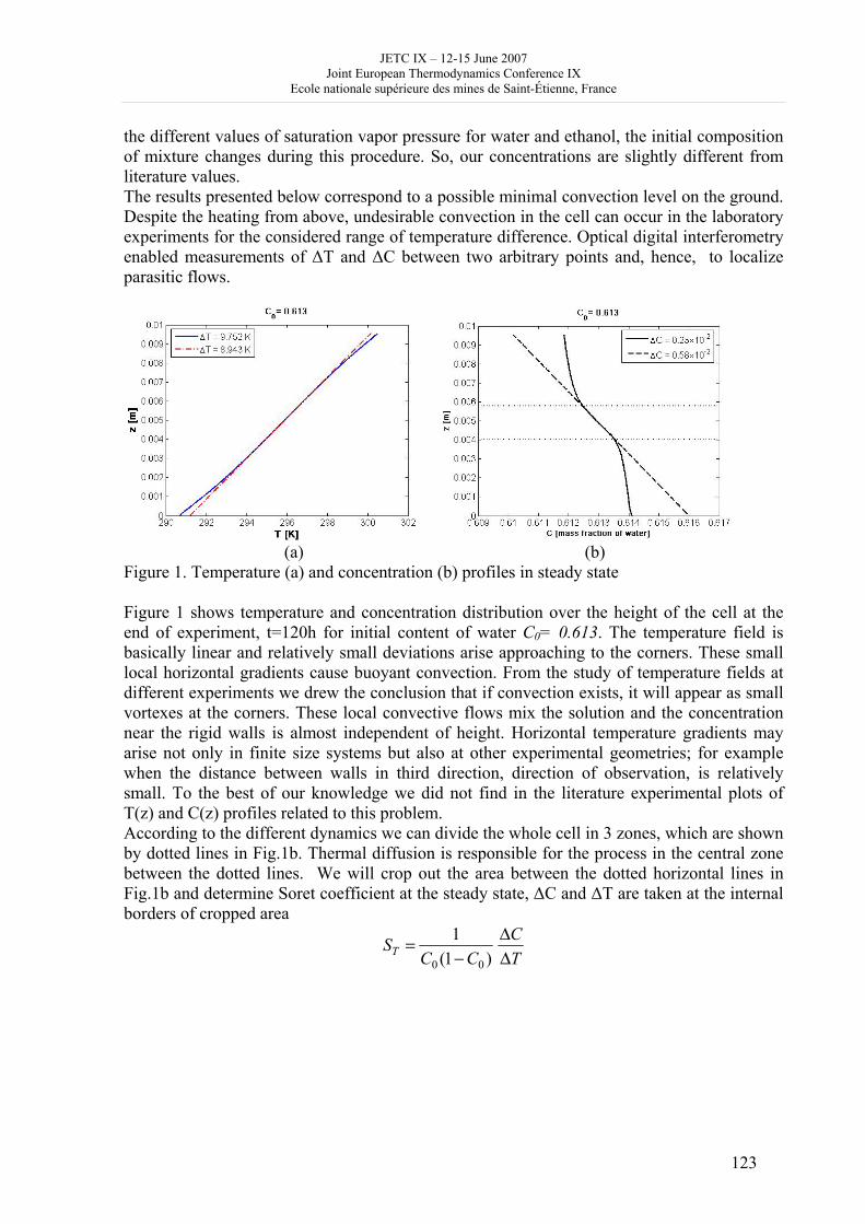
JETC IX – 12-15 June 2007 Joint European Thermodynamics Conference IX
Ecole nationale supérieure des mines de Saint-Étienne, France
123
the different values of saturation vapor pressure for water and ethanol, the initial composition of mixture changes during this procedure. So, our concentrations are slightly different from literature values. The results presented below correspond to a possible minimal convection level on the ground. Despite the heating from above, undesirable convection in the cell can occur in the laboratory experiments for the considered range of temperature difference. Optical digital interferometry enabled measurements of ΔT and ΔC between two arbitrary points and, hence, to localize parasitic flows.
(a) (b) Figure 1. Temperature (a) and concentration (b) profiles in steady state Figure 1 shows temperature and concentration distribution over the height of the cell at the end of experiment, t=120h for initial content of water C0= 0.613. The temperature field is basically linear and relatively small deviations arise approaching to the corners. These small local horizontal gradients cause buoyant convection. From the study of temperature fields at different experiments we drew the conclusion that if convection exists, it will appear as small vortexes at the corners. These local convective flows mix the solution and the concentration near the rigid walls is almost independent of height. Horizontal temperature gradients may arise not only in finite size systems but also at other experimental geometries; for example when the distance between walls in third direction, direction of observation, is relatively small. To the best of our knowledge we did not find in the literature experimental plots of T(z) and C(z) profiles related to this problem. According to the different dynamics we can divide the whole cell in 3 zones, which are shown by dotted lines in Fig.1b. Thermal diffusion is responsible for the process in the central zone between the dotted lines. We will crop out the area between the dotted horizontal lines in Fig.1b and determine Soret coefficient at the steady state, ΔC and ΔT are taken at the internal borders of cropped area
TC
CCST Δ
Δ−
=)1(
1
00
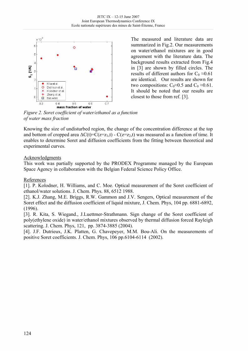
JETC IX – 12-15 June 2007 Joint European Thermodynamics Conference IX
Ecole nationale supérieure des mines de Saint-Étienne, France
124
The measured and literature data are summarized in Fig.2. Our measurements on water/ethanol mixtures are in good agreement with the literature data. The background results extracted from Fig.4 in [3] are shown by filled circles. The results of different authors for C0 ≈0.61 are identical. Our results are shown for two compositions: C0≈0.5 and C0 ≈0.61. It should be noted that our results are closest to those from ref. [3].
Figure 2. Soret coefficient of water/ethanol as a function of water mass fraction Knowing the size of undisturbed region, the change of the concentration difference at the top and bottom of cropped area ΔC(t)=C(z=z1,t) - C(z=z2,t) was measured as a function of time. It enables to determine Soret and diffusion coefficients from the fitting between theoretical and experimental curves. Acknowledgments This work was partially supported by the PRODEX Programme managed by the European Space Agency in collaboration with the Belgian Federal Science Policy Office. References [1]. P. Kolodner, H. Williams, and C. Moe. Optical measurement of the Soret coefficient of ethanol/water solutions. J. Chem. Phys. 88, 6512 1988. [2]. K.J. Zhang, M.E. Briggs, R.W. Gammon and J.V. Sengers, Optical measurement of the Soret effect and the diffusion coefficient of liquid mixture, J. Chem. Phys, 104 pp. 6881-6892, (1996). [3]. R. Kita, S. Wiegand., J.Luettmer-Strathmann. Sign change of the Soret coefficient of poly(ethylene oxide) in water/ethanol mixtures observed by thermal diffusion forced Rayleigh scattering. J. Chem. Phys, 121, pp. 3874-3885 (2004). [4]. J.F. Dutrieux, J.K. Platten, G. Chavepeyer, M.M. Bou-Ali. On the measurements of positive Soret coefficients. J. Chem. Phys, 106 pp.6104-6114 (2002).
JETC IX – 12-15 June 2007 Joint European Thermodynamics Conference IX
Ecole nationale supérieure des mines de Saint-Étienne, France
125
The arxim project: modules for the computation of thermodynamic equilibrium in heterogeneous systems;
applications to the simulation of fluid - rock systems
Jacques Moutte
Géochimie, Ecole des Mines de Saint Etienne, France
[email protected] Numerous computer programs are available for the calculation of thermodynamic equilibrium of heterogeneous systems, but it is often necessary to associate such calculations with other processes (e.g. kinetics, transport, ...), so that either several programs have to be used concurrently and "dynamically" exchange data, or, when using a more comprehensive software, rather complex scripts must be written. The objective of the arxim project is thus to develop, as an alternative to stand alone applications, a "library" of open, inter-dependent modules that comprise the main constructs and functions necessary for calculations of heterogeneous equilibrium in systems of arbitrary complexity. Originally developed as a "geochemical module" of a reactive transport code for water - rock interaction, the project is currently oriented toward fluid-rock systems, but its general architecture should be adaptable to a larger range of applications. The modules are written in Fortran 95, a language that, while suitable for the construction of complex codes, still remains readable for the non-professional programmer. The library consist of a hierarchy of data structures and related methods that implement the main constructs involved in chemical thermodynamics (component, species, phase, solution models, ...). As a result of this "encapsulation", adding new constructs, or extending the functionalities of a given construct is possible without reconsidering the whole program's structure. The "physical" modules, dedicated to the stoichiometric description of a system, the implementation of solution models, etc., are separated, as far as possible, from the more strictly numerical modules (e.g. matrix computations, implementation of a Newton-Raphson solver), in order to make easier the cooperative development between "physicists" and "numericists". Thermodynamic data can be retrieved from different types of sources, either from logK databases used by water-rock interaction softwares, or from more general tables of standard thermodynamic properties of pure and aqueous species. Modules are available for the implementation of the HKF equation of state [1,2], making arxim an intermediate between programs devoted to high (T,P) petrology [3,4] and those more oriented to fluid-rock interaction[5,6]. A stand alone application solving some problems of water-rock interactions is provided; it is used to check the modules' validity, but these are designed in such a way that any user can, on one hand, incorporate them in a specific application, and hopefully give feed back for their improvement, and, on the other hand, propose addition of new tools.

JETC IX – 12-15 June 2007 Joint European Thermodynamics Conference IX
Ecole nationale supérieure des mines de Saint-Étienne, France
126
Details on the project may be found on the web site www.emse.fr/~moutte/arxim References [1] Tanger J.C. IV, and Helgeson H.C., Amer. Jour. Science, 288: 19-98 (1988) [2] Johnson, J.W., Oelkers, E.H., and Helgeson H.C., Computers and Geosciences, (1992); updates at http://geopig.asu.edu/supcrt92_data/slop98.dat [3] de Capitani C., and Brown T.H., Geochim. Cosmochim. Acta 51:2639-2652 (1987) [4] Holland T.J.B. and Powell R., J. metamorphic Geol., 16: 309-343 (1998)
JETC IX – 12-15 June 2007 Joint European Thermodynamics Conference IX
Ecole nationale supérieure des mines de Saint-Étienne, France
127
Thermodynamic Optimization of Brayton Cycle with Steam Injection Using Exergy Analysis
M.Nikaien1, H.Ajam2, S.M.Hoseini Sarvari2
S.B University, Department of Mechanical Engineering, University St., Zahedan, Iran
[email protected] Gas turbine cycles, are suitable manner for fast power generation.But their efficiency is partly low.In order to achieving higher efficiencies, some propositions are preferred, such as recovery of heat from exhaust gases in a regenerator, utilization of intercooler in a multistage compressor ,steam injection to combustion chamber and etc. However, minimizing entropy generation of a cycle with these components is necessary for improving its efficiency. A.Poullikkas (2005), studied current and future sustainable gas turbine technologies [1].Ebadi et al (2005) studied exergetic analysis of gas turbine plants [2].In this research, thermodynamic optimization of a RISIGT1 cycle is presented. After recognition of most important effective parameters that affect on cycle proficiency-nominated as Design Parameters-such as compressor pressure ratio (RP), excess air in combustion (EA), turbine inlet temperature (TIT), rate of steam injection to combustion chamber (v), inlet air temperature (T0) and inlet air humidity ( )φ , entropy generation of RISIGT cycle (NS) derives as Objective Function using Exergy Analysis and Gouy-Stodola theorem. RISIGT cycle is shown in Fig.1.Our optimization problem and proper governing constraints, define as below: Minimize ( )φ,,,,, 0TvEATITRN Ps (1) Linear constraints:
501 ≤≤ PR , KTIT 16001000 ≤≤ , 41 ≤≤ EA 06.00 ≤≤ v , KT 323263 0 ≤≤ , 10 ≤≤ φ (2)
And nonlinear constraints: 0TTExh ≥ , (3)
This objective function minimized applying Genetic Algorithm in MATLAB. In this paper, we also peruse effect of regeneration, Intercooling and steam injection on optimum conditions and compute portion of each component in total entropy generation. Our main assumptions are: a) Air, combustion products and gaseous fuel are ideal gas with temperature dependent Cp. b) Fuel is natural gas with C1.5H5 chemical formula. c) Pressure drops in regenerator, intercooler and combustion chamber are considered. d) Compressor and turbine isentropic efficiencies and regenerator effectiveness are tc ηη ,
andε , respectively. e) Combustion chamber is not adiabatic, and combustion efficiency is bη . Results and conclusions 1. Combustion chamber and Stack are main elements in entropy generation, respectively. 2. RISIGT cycle has 43% more efficiency,51% more net power output and 22.2% less back
work ratio, in compare with simple gas turbine cycle.(When both of them work in optimum conditions)
3. Turbine entropy generation is more than compressor.
1 Regenerative-Intercooling-Steam-Injection-Gas- Turbine
intpodewExh TT ≥
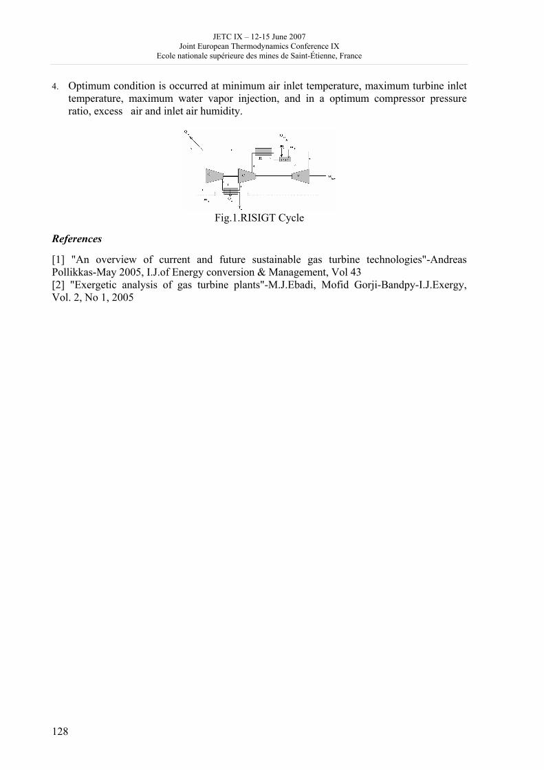
JETC IX – 12-15 June 2007 Joint European Thermodynamics Conference IX
Ecole nationale supérieure des mines de Saint-Étienne, France
128
4. Optimum condition is occurred at minimum air inlet temperature, maximum turbine inlet temperature, maximum water vapor injection, and in a optimum compressor pressure ratio, excess air and inlet air humidity.
Fig.1.RISIGT Cycle
References
[1] "An overview of current and future sustainable gas turbine technologies"-Andreas Pollikkas-May 2005, I.J.of Energy conversion & Management, Vol 43 [2] "Exergetic analysis of gas turbine plants"-M.J.Ebadi, Mofid Gorji-Bandpy-I.J.Exergy, Vol. 2, No 1, 2005
JETC IX – 12-15 June 2007 Joint European Thermodynamics Conference IX
Ecole nationale supérieure des mines de Saint-Étienne, France
129
A finite-time thermodynamics of unsteady flows from the onset of vortex shedding to developed homogeneous turbulence
Bernd R. Noack1, Michael Schlegel1, oye Ahlborn2, Gerd Mutschke3, Marek Morzynki4, Pierre Comte5 and Gilead Tadmor6
1 Berlin University of Technology, D-10623 Berlin, Germany 2 University of British Columbia, Vancouver V6Z 1Z1, Canada
3 Forschungszentrum Dresden-Rossendorf, Postfach 510119, D-01314 Dresden, Germany 4 Poznań University of Technology, PL-60-965 Poznań, Poland
5 Université de Poitiers, F-86036 Poitiers Cedex, France 6 Northeastern University, Boston, MA 02115, USA
[email protected] Abstract Turbulent fluid has often been conceptualized as transient thermodynamic phase. Here, a finite-time thermodynamics (FTT) formalism [1] is proposed to compute mean flow and fluctuation levels of unsteady incompressible flows. That formalism builds upon a traditional Galerkin model which simplifies a continuum 3D fluid motion into a finite-dimensional phase-space dynamics and subsequently, into a thermodynamics energy problem. This model consists of a velocity field expansion in terms of flow configuration dependent eigenmodes and of a dynamical system describing the temporal evolution of the mode coefficients. Each mode may be considered as a wave, parameterized by a wave number and frequency. In our FTT framework, the mode is treated as one thermodynamic degree of freedom, characterized by an energy level. The dynamical system approaches local thermal equilibrium (LTE) where each mode has the same energy if it is governed only by internal (triadic) mode interactions. However, the full system approaches only partial local thermal equilibrium (PLTE) by strongly mode-dependent external interactions. In these interactions, large-scale modes typically gain energy from the mean flow while small-scale modes loose energy to the heat bath. The energy flow cascade from large to small scales is thus a finite-time transition phenomenon. The FTT model has been successfully applied to predict the cascade for flows with simple to complex dynamics. Examples include laminar vortex shedding which is dominated by 2 eigenmodes and homogeneous shear turbulence which has been modeled with 1459 modes. In addition, the onset of vortex shedding is described in the Galerkin and vortex picture as a finite time scale phenomenon. 1. Introduction Turbulence is often referred to as the last unsolved problem of classical physics. As such, the quantitative description of fluid flows has been a tempting and rewarding challenge to many mathematics and physics disciplines, including theory of nonlinear dynamics, statistical physics and control theory, to name a few. Since the early 20th century, numerous studies propose a mathematical description of turbulence in the frame-work of statistical physics. While qualitative insights were gained, this approach has eluded a more rigorous quantitative prediction of flows. The statistical
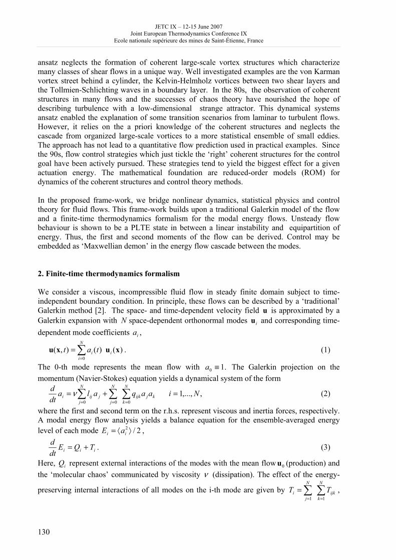
JETC IX – 12-15 June 2007 Joint European Thermodynamics Conference IX
Ecole nationale supérieure des mines de Saint-Étienne, France
130
ansatz neglects the formation of coherent large-scale vortex structures which characterize many classes of shear flows in a unique way. Well investigated examples are the von Karman vortex street behind a cylinder, the Kelvin-Helmholz vortices between two shear layers and the Tollmien-Schlichting waves in a boundary layer. In the 80s, the observation of coherent structures in many flows and the successes of chaos theory have nourished the hope of describing turbulence with a low-dimensional strange attractor. This dynamical systems ansatz enabled the explanation of some transition scenarios from laminar to turbulent flows. However, it relies on the a priori knowledge of the coherent structures and neglects the cascade from organized large-scale vortices to a more statistical ensemble of small eddies. The approach has not lead to a quantitative flow prediction used in practical examples. Since the 90s, flow control strategies which just tickle the ‘right’ coherent structures for the control goal have been actively pursued. These strategies tend to yield the biggest effect for a given actuation energy. The mathematical foundation are reduced-order models (ROM) for dynamics of the coherent structures and control theory methods. In the proposed frame-work, we bridge nonlinear dynamics, statistical physics and control theory for fluid flows. This frame-work builds upon a traditional Galerkin model of the flow and a finite-time thermodynamics formalism for the modal energy flows. Unsteady flow behaviour is shown to be a PLTE state in between a linear instability and equipartition of energy. Thus, the first and second moments of the flow can be derived. Control may be embedded as ‘Maxwellian demon’ in the energy flow cascade between the modes. 2. Finite-time thermodynamics formalism We consider a viscous, incompressible fluid flow in steady finite domain subject to time-independent boundary condition. In principle, these flows can be described by a ‘traditional’ Galerkin method [2]. The space- and time-dependent velocity field u is approximated by a Galerkin expansion with N space-dependent orthonormal modes iu and corresponding time-dependent mode coefficients ia ,
)()(),(0
xuxu i
N
ii tat ∑
=
= . (1)
The 0-th mode represents the mean flow with .10 ≡a The Galerkin projection on the momentum (Navier-Stokes) equation yields a dynamical system of the form
,,...,1000
Niaaqaladtd N
kkjijk
N
j
N
jjiji =+= ∑∑∑
===
ν (2)
where the first and second term on the r.h.s. represent viscous and inertia forces, respectively. A modal energy flow analysis yields a balance equation for the ensemble-averaged energy level of each mode 2/2 ⟩⟨= ii aE ,
iii TQEdtd += . (3)
Here, iQ represent external interactions of the modes with the mean flow 0u (production) and the ‘molecular chaos’ communicated by viscosity ν (dissipation). The effect of the energy-
preserving internal interactions of all modes on the i-th mode are given by ∑∑==
=N
kijk
N
ji TT
11
,
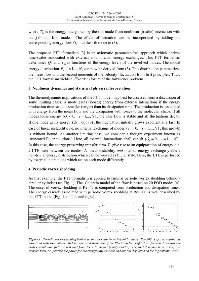
JETC IX – 12-15 June 2007 Joint European Thermodynamics Conference IX
Ecole nationale supérieure des mines de Saint-Étienne, France
131
where ijkT is the energy rate gained by the i-th mode from nonlinear (triadic) interaction with the j-th and k-th mode. The effect of actuation can be incorporated by adding the corresponding energy flow iG into the i-th mode in (3). The proposed FTT formalism [3] is an axiomatic parameter-free approach which derives time-scales associated with external amd internal energy exchanges. This FTT formalism determines iQ and ijkT as functions of the energy levels of the involved modes. The modal energy distribution ,,...,1, NiEi = can now be derived from (3). This distribution parametrizes the mean flow and the second moments of the velocity fluctuation from first principles. Thus, the FTT formalism yields a 2nd-order closure of the turbulence problem. 3. Nonlinear dynamics and statistical physics interpretation The thermodynamic implications of the FTT model may best be assessed from a discussion of some limiting cases. A mode gains (looses) energy from external interactions if the energy production time-scale is smaller (larger) than its dissipation time. The production is associated with energy from the mean flow and the dissipation with losses to the molecular chaos. If all modes loose energy ),...,1,0( NiQi =< , the base flow is stable and all fluctuations decay. If one mode gains energy )0:( >∃ iQi , the fluctuation initially grows exponentially fast. In case of linear instability, i.e. no internal exchange of modes ),...,1,0( NiTi == , this growth is without bound. As another limiting case, we consider a thought experiment known as ‘truncated Euler solutions’. Here, all external interactions shall vanish ),...,1,0( NiQi == . In this case, the energy-preserving transfer term iT give rise to an equipartition of energy, i.e. a LTE state between the modes. A linear instability and internal energy exchange yields a non-trivial energy distribution which can be viewed as PLTE state. Here, the LTE is perturbed by external interactions which act on each mode differently. 4. Periodic vortex shedding As first example, the FTT formalism is applied to laminar periodic vortex shedding behind a circular cylinder (see Fig. 1). The Galerkin model of the flow is based on 20 POD modes [4]. The onset of vortex shedding at Re=47 is computed from production and dissipation times. The energy cascade associated with periodic vortex shedding at Re=200 is well described by the FTT model (Fig. 1, middle and right).
Figure 1: Periodic vortex shedding behind a circular cylinder at Reynolds number Re=200. Left : a snapshot is visualized with streamlines. Middle: energy distribution of the POD modes. Right: transfer term from Navier-Stokes simulation (full circles) and from the FTT model (empty circles). The first 2 modes have a negative transfer term, i.e. provide the power for the energy flow cascade and are not displayed on the logarithmic scale.
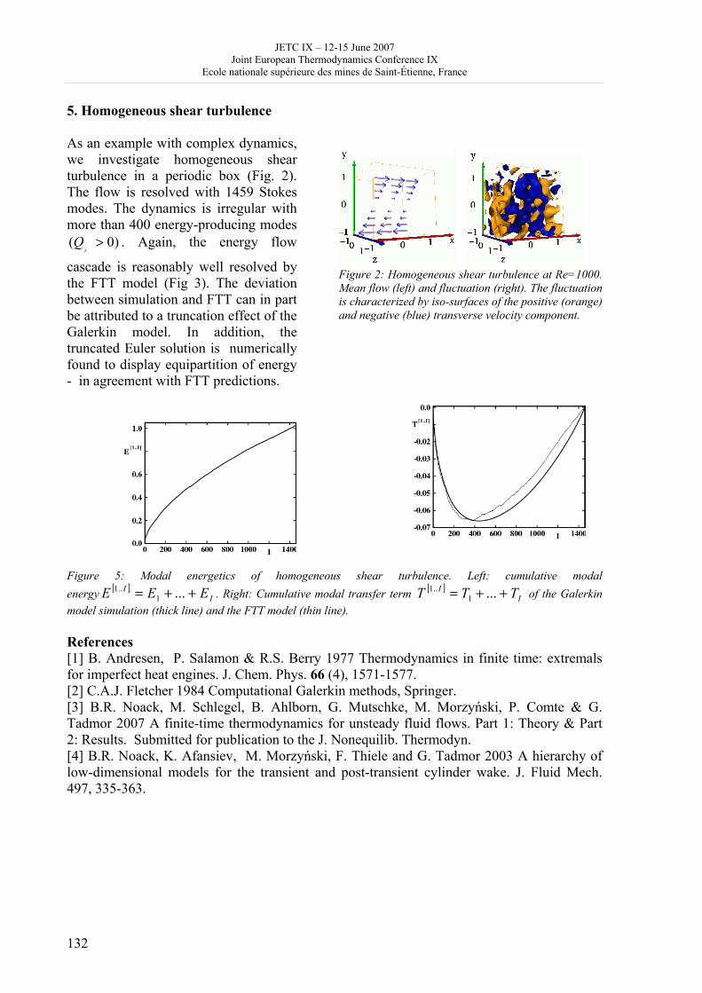
JETC IX – 12-15 June 2007 Joint European Thermodynamics Conference IX
Ecole nationale supérieure des mines de Saint-Étienne, France
132
5. Homogeneous shear turbulence As an example with complex dynamics, we investigate homogeneous shear turbulence in a periodic box (Fig. 2). The flow is resolved with 1459 Stokes modes. The dynamics is irregular with more than 400 energy-producing modes
)0( >i
Q . Again, the energy flow
cascade is reasonably well resolved by the FTT model (Fig 3). The deviation between simulation and FTT can in part be attributed to a truncation effect of the Galerkin model. In addition, the truncated Euler solution is numerically found to display equipartition of energy - in agreement with FTT predictions.
Figure 2: Homogeneous shear turbulence at Re=1000. Mean flow (left) and fluctuation (right). The fluctuation is characterized by iso-surfaces of the positive (orange) and negative (blue) transverse velocity component.
Figure 5: Modal energetics of homogeneous shear turbulence. Left: cumulative modal energy [ ]
II EEE ++= ...1
..1 . Right: Cumulative modal transfer term [ ]I
I TTT ++= ...1..1 of the Galerkin
model simulation (thick line) and the FTT model (thin line). References [1] B. Andresen, P. Salamon & R.S. Berry 1977 Thermodynamics in finite time: extremals for imperfect heat engines. J. Chem. Phys. 66 (4), 1571-1577. [2] C.A.J. Fletcher 1984 Computational Galerkin methods, Springer. [3] B.R. Noack, M. Schlegel, B. Ahlborn, G. Mutschke, M. Morzyński, P. Comte & G. Tadmor 2007 A finite-time thermodynamics for unsteady fluid flows. Part 1: Theory & Part 2: Results. Submitted for publication to the J. Nonequilib. Thermodyn. [4] B.R. Noack, K. Afansiev, M. Morzyński, F. Thiele and G. Tadmor 2003 A hierarchy of low-dimensional models for the transient and post-transient cylinder wake. J. Fluid Mech. 497, 335-363.
JETC IX – 12-15 June 2007 Joint European Thermodynamics Conference IX
Ecole nationale supérieure des mines de Saint-Étienne, France
133
A kinetic model for describing reactions between ideal solid solutions and aqueous solutions
E. Nourtier-Mazauric1, B. Guy2, D. Garcia2 1 Laboratoire Jean Kuntzmann, Grenoble, France
2 Ecole nationale supérieure des mines de Saint-Etienne, France
[email protected], [email protected], [email protected] In spite of the obvious importance of solid solutions in fluid-rock interactions, the kinetic approaches that have been proposed to incorporate those ubiquitous minerals in reactive transport models are few and recent [1,2]. In fact the continuously variable composition of solid solutions induces complex reactions when an aqueous solution is supersaturated with some solid solution. Indeed the range of solid compositions which can form changes as the aqueous solution evolves. This results in the coexistence of several precipitates, some of which must dissolve as the saturation state evolves. Therefore the reaction path may be very complex before equilibrium is reached at some unique solid and aqueous compositions. This study discusses especially kinetic aspects of the following theoretical and practical complications, in the case of ideal solid solutions: - departure from equilibrium is written differently depending on whether the composition of the solid solution is invariant or not, i.e. whether the stoichiometric saturation of the existing solid solution [3] or the total saturation if the whole range of potential compounds pertaining to the solid solution [4,5] is considered; - in general, equilibrium cannot be reached only by dissolving or precipitating the existing solid solution, and coprecipitation must be added to stoichiometric dissolution; when the aqueous solution is oversaturated with respect to a particular range of minerals pertaining to the solid solution, precipitation proceeds with a composition which is a priori different from that of the existing solid solution, and a rule must be introduced to calculate this composition as well as the reaction rate. The kinetic behaviour of an ideal solid solution is modelled here by two competing reactions: the stoichiometric dissolution of the existing solid and the (co-)precipitation of the least soluble compound, i.e. that with respect to which the oversaturation of the fluid is maximum. The overall reaction of the solid solution results from the simultaneous reactions of these two particular solid solutions, which are considered as independent, and they react with the fluid phase at their own rates: both reaction rates are expressed as a function of the corresponding departure from equilibrium. This defines uniquely how the fluid composition changes, how much of the existing solid solution is dissolved, and how much of the least soluble one is precipitated. This approach may be contrasted with the one followed by Lichtner and Carey [2], in which the solid solution is discretised into a finite set of stoichiometric solids with fixed compositions, and all supersaturated compositions may precipitate. Our work differs from theirs notably because in our approach, a single stoichiometric solid, corresponding to the least soluble phase, is allowed to precipitate. Moreover an oversimplification is done in our work in order to maintain a single phase (with varying composition and amount): the precipitate is assumed to dissolve immediately into the existing solid, which keeps a homogeneous composition instead of becoming zoned.
JETC IX – 12-15 June 2007 Joint European Thermodynamics Conference IX
Ecole nationale supérieure des mines de Saint-Étienne, France
134
In the binary case, chemical potential diagrams are introduced: they enable one to determine graphically the evolution of the solid solution composition from the aqueous one. References : [1] Nourtier-Mazauric, E., Guy, B., Fritz, B., Brosse, E., Garcia, D. and Clément, A., 2005. Modelling the dissolution/precipitation of ideal solid solutions. Oil & Gas Sci. And Tech. – Rev. IFP, 60, 2, 401-415. [2] Lichtner, P.C. and Carey, J.W., 2006. Incorporating solid solutions in reactive transport equations using a kinetic discrete-composition approach. Geochim. Cosmochim. Acta, 70, 1356-1378. [3] Thorstenson, D.C. and Plummer, L.N., 1977. Equilibrium criteria for two component solids reacting with fixed composition in aqueous phase. Example: the magnesian calcites. Am. J. Sci., 277, 1203-1223. [4] Denis, J. and Michard, G., 1983. Dissolution d'une solution solide : étude théorique et expérimentale. Bull. Minéral., 106, 309-319. [5] Michard, G., 1986. Dissolution d'une solution solide : compléments et corrections. Bull. Minéral., 109, 239-251.
JETC IX – 12-15 June 2007 Joint European Thermodynamics Conference IX
Ecole nationale supérieure des mines de Saint-Étienne, France
135
Recent advances in the use of the SAFT approach to Describe the Phase Behaviour of Associating Molecules, Electrolytes and Polymers.
Patrice Paricaud1*, Walter Furst 1, Christophe Coquelet2, Amparo Galindo3, George Jackson3. 1 Laboratoire de Chimie et Procédés, ENSTA, Paris, France; 2 Laboratoire de Thermodynamique des Equilibres de Phase,
Ecole des Mines de Paris, Fontainebleau. 3 Chemical Engineering Department, Imperial College, London, UK.
[email protected] A molecular description of matter using statistical mechanical theories and computer simulation modeling is the key to understanding and predicting the properties of dense fluids and materials. Fluid systems form an integral part of our modern lifestyle from the use of simple solvents in chemical processing to the design of opto-electronic devices with liquid crystalline and polymeric materials. The thermodynamics and phase equilibria of fluid systems are central to chemical process design in the traditional chemical and oil industries: calorimetry is used to design heat exchangers and refrigerators; separation and fractionation are important in distillation processes and the design of reaction stills; a knowledge of the thermodynamic properties of mixing is invaluable in choosing a solvent for a particular process; and an accurate description of phase and interfacial behaviour is of major interest in areas as diverse as supercritical fluid extraction of delicate substances, colloidal stability, detergency and enhanced oil recovery. In this contribution, we overview the recent developments in the use of the statistical associating fluid theory of variable range (SAFT-VR) in the areas of electrolytes, associating molecules with hydrogen bonding, and polymers. The focus will be on representative examples of: the use of SAFT together with a mean spherical approximation (MSA) treatment to examine the effect of added salt on the vapour–liquid equilibria (vapour pressure and density) of aqueous solutions of strong electrolytes; and the use of SAFT with parameters obtained for the long-chain alkanes to describe the adsorption and co-adsorption of alkanes and alkenes in polyethylene polymers. We will also discuss recent advances in the treatment of the near-critical region that requires the use of methodologies based on the renormalization group theory.
JETC IX – 12-15 June 2007 Joint European Thermodynamics Conference IX
Ecole nationale supérieure des mines de Saint-Étienne, France
136
From Dimer to Condensed Phases at Extreme Conditions: Accurate Predictions Properties of Water by a Gaussian Charge Polarizable Model
Patrice Paricaud1*, Jose L. Rivera2, Milan Předota3, Ariel A. Chialvo4, Peter T. Cummings4,5
1 Laboratoire de Chimie et Procédés, ENSTA, Paris, France; 2 Department of Physics, Wesleyan University, Middletown, CT, 06459, USA.
3 Department of Medical Physics and Biophysics, University of South Bohemia, Jírovcova 24, České Budějovice, 370 04, Czech Republic.
4 Chemical Sciences Division, Aqueous Chemistry and Geochemistry Group, Oak Ridge National Laboratory, Oak Ridge, Tennessee 37831-6110.
5 Department of Chemical Engineering, Vanderbilt University, Nashville, TN 37235-1604, USA.
[email protected] Water exhibits many unusual properties that are essential for the existence of life. Water completely changes its character from ambient to supercritical conditions, in a way that makes it possible to sustain life at extreme conditions, leading to conjectures that life may have originated in deep-sea vents. Molecular simulation can be very useful in exploring biological and chemical systems, particularly at extreme conditions for which experiments are either difficult or impossible; however this scenario entails an accurate molecular model for water applicable over a wide range of state conditions. Here, we present a Gaussian charge polarizable model (GCPM) based on the model developed earlier by Chialvo and Cummings (Fluid Phase Equilib. 150-151, 73 (1998)), which is, to our knowledge, the first that satisfies the water monomer and dimer properties, and simultaneously yields very accurate predictions of dielectric, structural, vapor-liquid equilibria, and transport properties, over the entire fluid range [1]. The particularity of the GCPM model is the use of Gaussian distributions instead of points to represent the partial charges on the water molecules. These charge distributions combined with a dipole polarizability and a Buckingham exp-6 potential are found to play a crucial role for the successful and simultaneous predictions of a variety of water properties. Some recent simulation results of the vapor-liquid interface of water are also presented. The different contributions of the surface tension were determined as well as the orientation profile of the water molecules and induce dipoles: it is found that the induced dipole has the same average orientation as the permanent dipole in the bulk phase, and but is more align to the interface than the permanent dipole in the interfacial regions [2].
References:
[1] P. Paricaud, M. Predota, A. A. Chialvo, P. T. Cummings, "From dimer to condensed phases at extreme conditions: Accurate predictions of the properties of water by a Gaussian charge polarizable model", J. Chem. Phys., 122, 244511 (2005). [2] J. L. Rivera, Francis W. Starr, P. Paricaud, and Peter T. Cummings, "Polarizable Contributions to the Surface Tension of Liquid Water", J. Chem. Phys., 125, 094712 (2006).
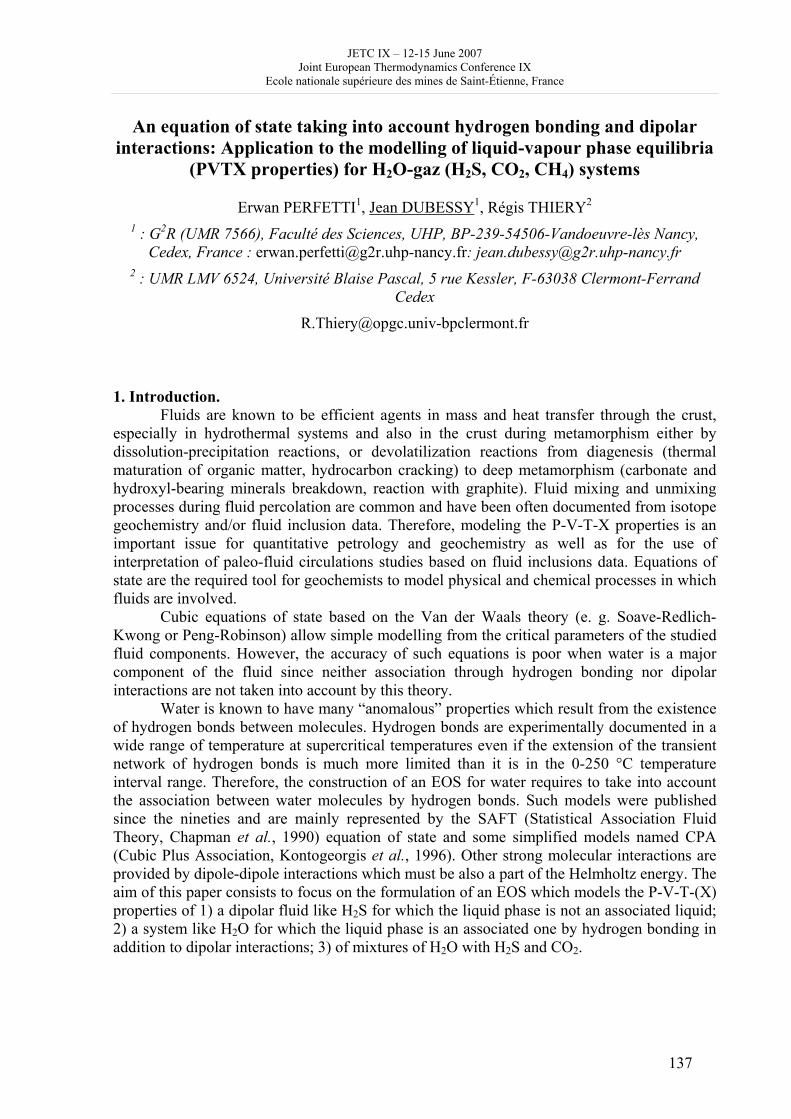
JETC IX – 12-15 June 2007 Joint European Thermodynamics Conference IX
Ecole nationale supérieure des mines de Saint-Étienne, France
137
An equation of state taking into account hydrogen bonding and dipolar interactions: Application to the modelling of liquid-vapour phase equilibria
(PVTX properties) for H2O-gaz (H2S, CO2, CH4) systems
Erwan PERFETTI1, Jean DUBESSY1, Régis THIERY2 1 : G2R (UMR 7566), Faculté des Sciences, UHP, BP-239-54506-Vandoeuvre-lès Nancy,
Cedex, France : [email protected]: [email protected] 2 : UMR LMV 6524, Université Blaise Pascal, 5 rue Kessler, F-63038 Clermont-Ferrand
Cedex
[email protected] 1. Introduction. Fluids are known to be efficient agents in mass and heat transfer through the crust, especially in hydrothermal systems and also in the crust during metamorphism either by dissolution-precipitation reactions, or devolatilization reactions from diagenesis (thermal maturation of organic matter, hydrocarbon cracking) to deep metamorphism (carbonate and hydroxyl-bearing minerals breakdown, reaction with graphite). Fluid mixing and unmixing processes during fluid percolation are common and have been often documented from isotope geochemistry and/or fluid inclusion data. Therefore, modeling the P-V-T-X properties is an important issue for quantitative petrology and geochemistry as well as for the use of interpretation of paleo-fluid circulations studies based on fluid inclusions data. Equations of state are the required tool for geochemists to model physical and chemical processes in which fluids are involved. Cubic equations of state based on the Van der Waals theory (e. g. Soave-Redlich-Kwong or Peng-Robinson) allow simple modelling from the critical parameters of the studied fluid components. However, the accuracy of such equations is poor when water is a major component of the fluid since neither association through hydrogen bonding nor dipolar interactions are not taken into account by this theory. Water is known to have many “anomalous” properties which result from the existence of hydrogen bonds between molecules. Hydrogen bonds are experimentally documented in a wide range of temperature at supercritical temperatures even if the extension of the transient network of hydrogen bonds is much more limited than it is in the 0-250 °C temperature interval range. Therefore, the construction of an EOS for water requires to take into account the association between water molecules by hydrogen bonds. Such models were published since the nineties and are mainly represented by the SAFT (Statistical Association Fluid Theory, Chapman et al., 1990) equation of state and some simplified models named CPA (Cubic Plus Association, Kontogeorgis et al., 1996). Other strong molecular interactions are provided by dipole-dipole interactions which must be also a part of the Helmholtz energy. The aim of this paper consists to focus on the formulation of an EOS which models the P-V-T-(X) properties of 1) a dipolar fluid like H2S for which the liquid phase is not an associated liquid; 2) a system like H2O for which the liquid phase is an associated one by hydrogen bonding in addition to dipolar interactions; 3) of mixtures of H2O with H2S and CO2.
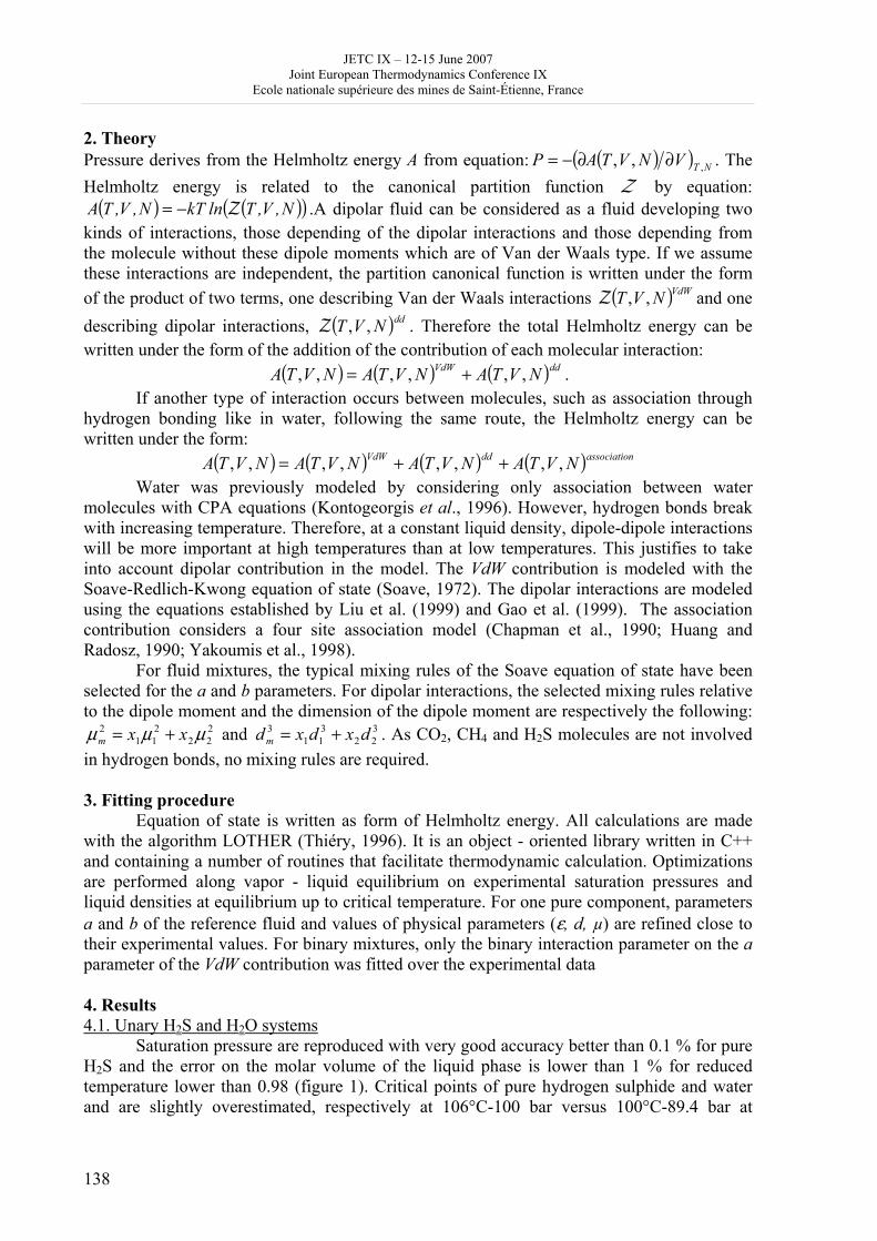
JETC IX – 12-15 June 2007 Joint European Thermodynamics Conference IX
Ecole nationale supérieure des mines de Saint-Étienne, France
138
2. Theory Pressure derives from the Helmholtz energy A from equation: ( )( ) NTVNVTAP ,,, ∂∂−= . The Helmholtz energy is related to the canonical partition function Z by equation:
( ) ( )( )N,V,TlnkTN,V,TA Z−= .A dipolar fluid can be considered as a fluid developing two kinds of interactions, those depending of the dipolar interactions and those depending from the molecule without these dipole moments which are of Van der Waals type. If we assume these interactions are independent, the partition canonical function is written under the form of the product of two terms, one describing Van der Waals interactions ( )VdWNVT ,,Z and one describing dipolar interactions, ( )ddNVT ,,Z . Therefore the total Helmholtz energy can be written under the form of the addition of the contribution of each molecular interaction:
( ) ( ) ( )ddVdW NVTANVTANVTA ,,,,,, += . If another type of interaction occurs between molecules, such as association through hydrogen bonding like in water, following the same route, the Helmholtz energy can be written under the form:
( ) ( ) ( ) ( ) nassociatioddVdW NVTANVTANVTANVTA ,,,,,,,, ++= Water was previously modeled by considering only association between water molecules with CPA equations (Kontogeorgis et al., 1996). However, hydrogen bonds break with increasing temperature. Therefore, at a constant liquid density, dipole-dipole interactions will be more important at high temperatures than at low temperatures. This justifies to take into account dipolar contribution in the model. The VdW contribution is modeled with the Soave-Redlich-Kwong equation of state (Soave, 1972). The dipolar interactions are modeled using the equations established by Liu et al. (1999) and Gao et al. (1999). The association contribution considers a four site association model (Chapman et al., 1990; Huang and Radosz, 1990; Yakoumis et al., 1998). For fluid mixtures, the typical mixing rules of the Soave equation of state have been selected for the a and b parameters. For dipolar interactions, the selected mixing rules relative to the dipole moment and the dimension of the dipole moment are respectively the following:
222
211
2 μμμ xxm += and 322
311
3 dxdxdm += . As CO2, CH4 and H2S molecules are not involved in hydrogen bonds, no mixing rules are required. 3. Fitting procedure Equation of state is written as form of Helmholtz energy. All calculations are made with the algorithm LOTHER (Thiéry, 1996). It is an object - oriented library written in C++ and containing a number of routines that facilitate thermodynamic calculation. Optimizations are performed along vapor - liquid equilibrium on experimental saturation pressures and liquid densities at equilibrium up to critical temperature. For one pure component, parameters a and b of the reference fluid and values of physical parameters (ε, d, µ) are refined close to their experimental values. For binary mixtures, only the binary interaction parameter on the a parameter of the VdW contribution was fitted over the experimental data 4. Results 4.1. Unary H2S and H2O systems Saturation pressure are reproduced with very good accuracy better than 0.1 % for pure H2S and the error on the molar volume of the liquid phase is lower than 1 % for reduced temperature lower than 0.98 (figure 1). Critical points of pure hydrogen sulphide and water and are slightly overestimated, respectively at 106°C-100 bar versus 100°C-89.4 bar at
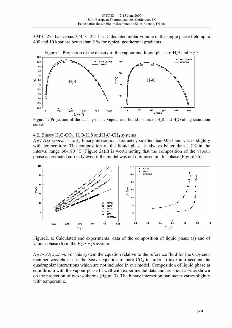
JETC IX – 12-15 June 2007 Joint European Thermodynamics Conference IX
Ecole nationale supérieure des mines de Saint-Étienne, France
139
394°C-275 bar versus 374 °C-221 bar. Calculated molar volume in the single phase field up to 400 and 10 kbar are better than 2 % for typical geothermal gradients.
Figure 1: Projection of the density of the vapour and liquid phase of H2S and H2O.
Figure 1: Projection of the density of the vapour and liquid phases of H2S and H2O along saturation curves. 4.2. Binary H2O-CO2, H2O-H2S and H2O-CH4 systems H2O-H2S system. The kij binary interaction parameter, smaller than0.023 and varies slightly with temperature. The composition of the liquid phase is always better than 1.7% in the interval range 60-180 °C (Figure 2a).It is worth noting that the composition of the vapour phase is predicted correctly even if the model was not optimised on this phase (Figure 2b).
Figure2. a: Calculated and experimental data of the composition of liquid phase (a) and of vapour phase (b) in the H2O-H2S system. H2O-CO2 system. For this system the equation relative to the reference fluid for the CO2-end-member was chosen as the Soave equation of pure CO2 in order to take into account the quadrupolar interactions which are not included in our model. Composition of liquid phase at equilibrium with the vapour phase fit well with experimental data and are about 5 % as shown on the projection of two isotherms (figure 3). The binary interaction parameter varies slightly with temperature.
H2O H2S
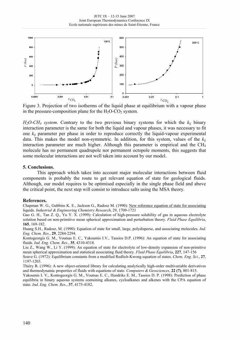
JETC IX – 12-15 June 2007 Joint European Thermodynamics Conference IX
Ecole nationale supérieure des mines de Saint-Étienne, France
140
Figure 3. Projection of two isotherms of the liquid phase at equilibrium with a vapour phase in the pressure-composition plane for the H2O-CO2 system. H2O-CH4 system. Contrary to the two previous binary systems for which the kij binary interaction parameter is the same for both the liquid and vapour phases, it was necessary to fit one kij parameter per phase in order to reproduce correctly the liquid-vapour experimental data. This makes the model non-symmetric. In addition, for this system, values of the kij interaction parameter are much higher. Although this parameter is empirical and the CH4 molecule has no permanent quadrupole nor permanent octopole moments, this suggests that some molecular interactions are not well taken into account by our model. 5. Conclusions. This approach which takes into account major molecular interactions between fluid components is probably the route to get relevant equation of state for geological fluids. Although, our model requires to be optimised especially in the single phase field and above the critical point, the next step will consist to introduce salts using the MSA theory. References. Chapman W. G., Gubbins K. E., Jackson G., Radosz M. (1990): New reference equation of state for associating liquids. Industrial & Engineering Chemistry Research, 29, 1709-1721 Gao G. H., Tan Z. Q., Yu Y. X. (1999): Calculation of high-pressure solubility of gas in aqueous electrolyte solution based on non-primitive mean spherical approximation and perturbation theory. Fluid Phase Equilibria, 165, 169-182. Huang S.H., Radosz, M. (1990): Equation of state for small, large, polydisperse, and associating molecules. Ind. Eng. Chem. Res., 29, 2284-2294. Kontogeorgis G. M., Voutsas E. C., Yakoumis I.V., Tassios D.P. (1996): An equation of state for associating fluids. Ind. Eng. Chem. Res., 35, 4310-4318. Liu Z., Wang W., Li Y. (1999): An equation of state for electrolyte of low-density expansion of non-primitive mean spherical approximation and statistical associating fluid theory. Fluid Phase Equilibria, 227, 147-156 Soave G. (1972): Equilibrium constants from a modified Redlich-Kwong equation of states. Chem. Eng. Sci., 27, 1197-1203. Thiéry R. (1996): A new object-oriented library for calculating analytically high-order multivariable derivatives and thermodynamic properties of fluids with equations of state. Computers & Geosciences, 22 (7), 801-815. Yakoumis I. V., Kontogeorgis G. M., Voutsas E. C., Hendriks E. M., Tassios D. P. (1998): Prediction of phase equilibria in binary aqueous systems containing alkanes, cycloalkanes and alkenes with the CPA equation of state. Ind. Eng. Chem. Res., 37, 4175-4182.
JETC IX – 12-15 June 2007 Joint European Thermodynamics Conference IX
Ecole nationale supérieure des mines de Saint-Étienne, France
141
Some Problems in the Teaching of Thermodynamics
Pierre Perrot
Laboratoire de Métallurgie Physique, Université des Sciences et technologies de Lille
[email protected] Introduction
Who did not experience the following situations? Being given an equilibrium of the kind:
Ice + Cream Icecream, characterized by K(T) = [Icecream] / [Ice][Cream],
what happens if [Cream] is multiplied by λ? The immediate answer is “Stupid question! The equilibrium constant K is indeed divided by λ!”☺. Here is another situation about the well-known expression giving the Gibbs energy of a reaction: ΔrG = ΔrG° + R T ln K! What is K ? “Is it necessary to ask for? K is the equilibrium constant, of course!”☺ I have pointed out a lot of mistakes in thermodynamics textbooks, and I have never seen such an affirmation, but it is surely impressed in gold letters into the students’ brains because I have even seen it on a poster in an international conference! It is easy to find some reasons for such a lack of a deep understanding: Thermodynamics makes a big use of differential quantities and most of the students (I dare not say most of the teachers), victims of what may be called “mathematical terrorism”, consider thermodynamics as the art of handling differential equations. Every undergraduate student is able to integrate elegantly the Clapeyron’s equation, but unable to answer even a simple question about the physical meaning of the obtained curves! The aim of this presentation is to pin point the looseness of terminology, the vagueness of statements, the unproved affirmations which make thermodynamics look like an esoteric science in which only initiated people may feel at ease! The principles
Thermodynamics did not arise like Aphrodite in all her glory out of the sea-foam, but blossomed gently, developing during the nineteenth century and reaching its full flowering during the first half of the twentieth century. The word itself was coined by Joule in 1858 to designate the science of relations between heat (θερμη) and power (δυναμις). Of course, classical phenomenon in history of sciences, its subject matter quickly expanded and thermodynamics designates now the science of all transformations of matter and energy. It rests on four principles clearly explicated by Clausius in 1850 (First and second law), Maxwell in 1872 (Zeroth law) and Nernst in 1918 (Third law). Epistemologists think that four principles for the ground of a science, it is may be three too much, and, in 1972, Hatsopoulos and Keenan showed that thermodynamics may be based on a single principle called “Law of stable equilibrium”, which may be expressed by a very simple, elegant and understandable statement: A constrained system, evolving in such a way that its surroundings remain unmodified, can reach one and only one state of stable equilibrium. Each word is important, but developing thermodynamics from this simple statement is not the easiest, neither the most pedagogical way to be understandable. The four old principles have still happy days before them. Neither the zeroth law, which is an easy mean to introduce the concept of temperature, neither the third law which defines an absolute value for the entropy function raises many problems, so, we shall focus our attention on the two first laws of thermodynamics
JETC IX – 12-15 June 2007 Joint European Thermodynamics Conference IX
Ecole nationale supérieure des mines de Saint-Étienne, France
142
The first law
The first law states, a little too quickly, that neither the elemental work dW, neither the elemental heat dQ are exact differential, whereas their sum dU = dQ + dW is an exact differential. In other terms, a system cannot be defined by its work content W, neither by its heat content Q because the functions W and Q do not exist. On another hand, a system can be defined by its internal energy U because the function U exists. The difficulties arise when we try to develop dW under the form: dW = ∑ Yi dXi where Xi and Yi are an extensity and a tension, respectively.
What is an extensity (or an extensive quantity)? It is a quantity proportional to the dimension of the system: Example: a length l, a surface A, a volume V, a quantity of electricity q or a quantity of matter ni. No problem? No problems! OK.
What is a tension? It is the partial derivative of an internal energy with respect to an extensity! As a consequence, a tension is an intensive quantity which may be defined for each point in the space. Example: A temperature T, a force F, a surface tension σ, a pressure P, an electric tension E, a chemical potential µi. No Problem? Wait a minute!
When two systems A and B interact, the assembly (A+B) being isolated, the energy exchanged under the influence of a difference in tension is manifested by a transfer of extensity. The greater the difference in tension between A and B, the greater is the flux of extensity crossing the boundary. So, the important consequence of the definition of a tension is the following: Tensions measured on both sides of the boundary separating two systems at equilibrium are equal.
With that result in mind, it is easy to develop:
dW = F dl + σ dA − P dV + E dq + ∑ µi dni
Such a development is satisfying if we do not try to include dEk (kinetical energy) neither dEp (potential energy) in the development of dW, because it is impossible to decompose an expression of dEk or dEp as the product of a tension by an extensity. This is impossible because Ek and Ep are not internal energy (Internal energy of a system depends only on the microscopic parameters of the system), but external energy (External energy of a system depends on its macroscopic parameters and on its coordinates in an external field).
The best expression of the first law is the following : There is a state function E, called “energy”, whose differential equals the work exchanged with the surroundings during an adiabatic process.
This statement needs only to define beforehand the concept of work and to give the meaning of the word adiabatic. The corollary, which states that E defined by:
dE = dQ + dW
is a state function is often presented as the first law, which is quite legitimate, but which suppose that heat has been defined beforehand, independently of the first law.
The energy E has two contributions: the internal energy U and the external energy which has itself a kinetic and a potential contribution:
dE = dU + dEk + dEp
As Ek and Ep are functions of state (dEk and dEp are exact differentials), U is also a function of state (dU is an exact differential). A tension is the derivative of U with respect to an extensity.
JETC IX – 12-15 June 2007 Joint European Thermodynamics Conference IX
Ecole nationale supérieure des mines de Saint-Étienne, France
143
What is the statute of electric or magnetic energies? Authors generally avoids taking a position; those who come to a decision generally class these energies as internal energies without too much justification, even if the electric work classically expressed by dW = ΔE dq (the potential of an electric charge dq varies by ΔE ) is clearly internal energy. Actually, an acute analysis of the situation shows that both energies have an internal and an external contribution. The fundamental reason proceeds from the fact that the presence of matter in an electric or in a magnetic field modifies these fields, which is not the case for a gravitational field.
The external contribution of electric energy, electrostatic energy of vacuum due to fixed charges is a potential energy expressed by dW = εo E dE (εo and E are the permittivity of the vacuum and the electric field, respectively). The external contribution of magnetic energy, the magnetic energy of vacuum due to electric current, is a kinetic energy expressed by dW = μo H dH (µo and H are the permeability of the vacuum and the magnetic excitation, respectively).
The second law
It is possible to present at least 30 different statements for the second law, the best known being those of Carnot, Clausius, Planck and Caratheodory. Once a statement accepted, the other may be deduced. Some statements do not use the concept of entropy. The entropy and its properties are then derived as a consequence of the second law. Most recent textbooks prefer first to define the entropy, then states the second law as a property of entropy which easily understandable, for instance: The entropy of an isolated system increases and reaches a maximum which corresponds to an equilibrium state.
In the short time available for this presentation, I forgot the 31th statement of the second law, that of Boltzmann, which is very different, because it does not forbid a decrease of the entropy of an isolated system, but gives a probability for the occurrence of such an event. I want only to show why, even very clever students cannot understand the concept of entropy. When the greek or latin tragedians did not know how to end a story, they introduced the Deus ex Machina. More than 2000 years later, the situation did not evolve very much: when modern authors of textbooks do not know how to present the concept of entropy, they use an undisputed authority: that of Prigogine : It exists a function entropy, labeled S, depending on the state of the system and which is defined by dS = (dQ/T)rev. Poor Prigogine! Did he know how many nonsense were expressed on his behalf?
Actually, the best way to present quickly the concept of entropy is to proceed by steps, showing successively that:
• dQ is not an exact differential (by a thought experiment)
• dQ / T is not an exact differential (by a thought experiment)
• For the transformations called reversible, dQ / T is a total differential.
This last statement is a theorem, which means that it may be rigorously demonstrated provided that a reversible transformation be carefully defined, which occurs rarely. The demonstration seems hard to understand because it cannot be carried out by a thought experiment, hence he reason why it is never encountered in the textbooks.
If (dQ / T )rev is an exact differential, it is possible to give a name (entropy) and a symbol (S) to the function whose the differential is dS = (dQ / T )rev. In simple words, the function 1 / T is not the integrating factor of dQ, but the integrating factor of dQrev.
JETC IX – 12-15 June 2007 Joint European Thermodynamics Conference IX
Ecole nationale supérieure des mines de Saint-Étienne, France
144
Once recognized the entropy function, it is possible to introduce the second law. It seems artificial to present the second law as an increase of entropy for an isolated system. It is less abrupt to identify the second law with the Clausius’inequality:
dS = (dQ / T )rev > (dQ / T )irr
Thought experiments show that Clausius’ inequality is obeyed in many cases, but they cannot be a proof that the inequality is always verified. As its generalization cannot be rigorously demonstrated, it is accepted as the “second law” whose correctness is verified by the exactitude of its consequences. As inequalities are not very praised by the human brain, the second law is better presented by the following equation:
dS = (dQ / T ) + d σ
where dσ, entropy created by the irreversibility of the transformation, is positive for an irreversible transformation (which is the second law) and zero for a reversible transformation (which is a well demonstrated theorem). An alternative, but similar presentation is to separate the entropy change into two contributions dS = deS + diS :
• deS = dQ / T, external contribution to the entropy change, represents a flux term
• diS = dσ ≥ 0, internal contribution to the entropy change, represents a source term
The introduction of the Helmholtz and Gibbs functions follows easily.
The chemical potential
It exists, in thermodynamics, few “magic formula” such as:
µi = µi° + R T ln ai
E = E° + ( R T / n F ) ln [(Ox) / (Red)]
ΔrG = ΔrG° + R T ln Π (ai)νi
These formula are “magic” because they can be easily proved, need no approximation, so that they are often used without any consideration about their physical meaning. Their presentation need few pages in thermodynamic textbooks (actually, few lines would be enough with underlying idea well understood), thus missing the most important features amongst their common characteristics. These three equations present the same construction: a first member which represents the result of a physical measure on a real system and a second member which is the sum of two terms. The first terms of the second members depend only on arbitary choosen standard states, whereas the second terms of the second members depends not only on the standard states, but also on the physical state of the system under investigation. As a consequence, any change in the standard states modify both terms of the second members, but these modifications annihilates because the first member represents a physical quantity measured by a physicist or a chemist and cannot be dependent on the arbitary choice of a standard state. This fact is never explicited so that, we can admire the types of poetry shown in the beginning of the presentation. There is a very nice problem which put in stage the inhabitants of two lovely planets: Melpomene and Proserpine. Their choice of standard states are linked to the physical characteristics of their own planets, so that thermodynamic tables are very different in both planets. Equilibrium constants calculated on each planet are, of course, far from being the same, but calculations give exactly the same results for the same physical conditions on both planets!
JETC IX – 12-15 June 2007 Joint European Thermodynamics Conference IX
Ecole nationale supérieure des mines de Saint-Étienne, France
145
Great confusions arise about the concept of chemical potential when a system exchanges an electrical work with the surroundings. It is traditional among electrochemists to define an electrochemical potential:
Φ+= Fiii zµµ~
where F is the Faraday’s constant and Φ the Galvani’s Potential. A close examination shows that the so called electrochemical potential is the new name of the chemical potential which has been separated into a chemical contribution µi and an electrical contribution zi F Φ. One must be aware of the implications of this new jargon. Only the electrochemical potential iµ~ is a quantity of tension because the equilibrium between two phases is expressed by equalling the electrochemical potentials iµ~ , not the chemical contribution µi. Conclusions
The presentation remains in the field of the macroscopic thermodynamics for the use of undergraduate students. It points out the “mathematical terrorism”, which favors the formal developments at the expense of the physical meaning of equations used, whence the low scientific rigor and sometimes the big mistakes due to the lack of understanding of fundamental concepts encountered in many textbooks. Paradoxes encountered in thermodynamics may be usefully discussed as good mental exercises to check ones profound understanding of the phenomena. Most of them are false paradoxes, reducing the second law to “Entropy may only increase”, forgetting that it is only valid for an isolated system. Considerations about the appearance of complex structures on the earth or in the Universe belong to this kind of fallacious paradoxes. Some paradoxes raise more serious objections and deserve careful discussion. Amongst the best known may be mentioned the Gibbs paradox, Maxwell’ demon, Poincaré recurrence, Speed inversion, Levenspiel’s fountain
JETC IX – 12-15 June 2007 Joint European Thermodynamics Conference IX
Ecole nationale supérieure des mines de Saint-Étienne, France
146
Study of the thermal diffusion behaviour of alkane/benzene mixtures by Thermal Diffusion Forced Rayleigh Scattering experiments and lattice
model calculations
Pavel Polyakov1, Jutta Luettmer-Strathmann2 and Simone Wiegand1 1 Forschungszentrum Juelich GmbH, IFF - Weiche Materie, D-52428 Juelich, Germany
2 Department of Physics and Department of Chemistry, The University of Akron, Akron, Ohio 44325-4001
[email protected] Introduction Thermal diffusion or the so-called Ludwig-Soret effect describes the coupling between a temperature gradient and a resulting mass flux. The effect has important technical applications for example in the modelling of the separation of crude oil components under the influence of thermal diffusion in geological conditions [1]; it also plays an important role in separation techniques for liquid mixtures (see e.g. Refs.[2-4]). Thermal diffusion in liquid mixtures of non-polar fluids is known to reflect a range of microscopic properties such as the mass, size, and shape of the molecules as well as their interactions (see Ref. [4] for a review). In mixtures of polar liquids, specific interactions between the molecules dominate the thermal diffusion process while mass and size of the molecules are most important in Lennard-Jones fluids. For liquids of non-polar molecules that are more complex than Lennard-Jones fluids, the Soret effect appears to depend on a delicate balance of the molecular properties of the components. This is true, in particular, for mixtures of alkanes and aromatic solvents. The group of Köhler [5, 6] investigated thermal diffusion in isotopic mixtures of benzene and other organic compounds with cyclohexane and wrote the Soret coefficient as a sum of three contributions:
δST = aM δM + bI δI + ST0 ,
where δM=(M1-M2) and δI=(I1-I2) are the absolute differences in mass and in moment of inertia (I1, I2). The coefficients aM and bI were found to be independent of the composition of the mixture. The third contribution, ST
0, reflects chemical differences of the molecules and was found to depend on the concentration and change its sign at a benzene mole fraction of 0.7. A further investigation of the isotope effect [6] suggested that the change of ST after isotopic substitution of cyclohexane neither depends on concentration nor on the nature of the non-polar mixing partner. We focus in this work on the Soret effect in binary alkane/benzene mixtures for linear as well as branched alkanes at different temperatures and concentrations. For the n-alkanes, we expect the differences in the chain length (molecular mass) to have the largest effect; for the branched alkanes, we expect a significant effect due to differences in the molecular architecture and the corresponding changes in the moments of inertia. Isotopic shift of ST for n-alkane/benzene mixtures after C6H6 to C6D6 substitution was investigated additionally. In order to investigate with theoretical methods the effect of intermolecular interactions on thermal diffusion, we have adapted a recently developed two-chamber lattice model for thermodiffusion [7] to alkane/benzene mixtures. In the two-chamber lattice model, one considers a lattice system divided into two chambers of equal size that are maintained at slightly different temperatures. Particles are free to move between the chambers, which do not otherwise interact. The partition functions for the chambers are calculated in exact
JETC IX – 12-15 June 2007 Joint European Thermodynamics Conference IX
Ecole nationale supérieure des mines de Saint-Étienne, France
147
enumeration and combined to yield a sum of states for the system. The Soret coefficient is then determined from the difference in average composition of the solutions in the two chambers. The system-dependent parameters of the model are determined from a comparison with thermodynamic properties of the pure components and volume changes on mixing. This allows us to make predictions of the Soret coefficient as a function of temperature, pressure, and composition without adjustable parameters. We find that predictions from this model, which includes the effects of chain length of the alkanes and orientation-dependent interactions of benzene molecules, are in good qualitative agreement with the Soret coefficients of linear alkane chains in benzene. Experiment Sample preparation The alkanes heptane (99,5 %), nonane (99 %), undecane (98 %), 2-methylhexane (98 %), 3-methylhexane (98 %) and 2,2,3-trimethylbutane (99 %) were purchased from Fluka; tridecane (99 %), pentadecane (99 %), heptadecane (99 %), 2,3-dimethylpentane (99 %), 2,4-dimethylpentane (99 %), 2,2,4-trimethylpentane (99 %), benzene (99.7 %) and deuterated benzene (96.96 atom % D) were ordered from Aldrich. The alkane mole fraction for all mixtures was adjusted by weighing the components. All samples contained approximately 0.002 wt % of the dye Quinizarin (Aldrich). Before each TDFRS experiment, approximately 2 ml of the freshly prepared solution were filtered through 0.2 μm filter (hydrophobic PTFE) into an optical quartz cell with 0.2 mm optical path length (Helma) which was carefully cleaned from dust particles before usage. TDFRS experiment and data analysis In our thermal diffusion forced Raleigh scattering (TDFRS) experiments, the beam of an argon-ion laser (λw=488 nm) is split into two writing beams of equal intensity which are allowed to interfere in the sample cell (see Ref. [8] for a detailed description of the method). A small amount of dye is present in the sample and converts the intensity grating into a temperature grating, which in turn causes a concentration grating by the effect of thermal diffusion. Both gratings contribute to a combined refractive index grating, which is read out by Bragg diffraction of a third laser beam (λr=633 nm). Results In Fig. 1 we present Soret coefficients of heptane and tridecane in mixtures with benzene as a function of composition for three different temperatures. The symbols are connected by dashed lines represent experimental data while the solid lines represent calculated Soret coefficients. The negative Soret coefficient implies that the linear alkane molecules tend to move to the warmer regions of the fluid while the benzene molecules tend to move in the opposite direction. Both theory and experiment show an increase of the alkane Soret coefficients with increasing alkane mole fraction, x. They also show that the temperature dependence of the Soret effect is larger for benzene-rich mixtures than for alkane rich mixtures. The differences between calculated and experimental values are most pronounced for alkane-rich mixtures.
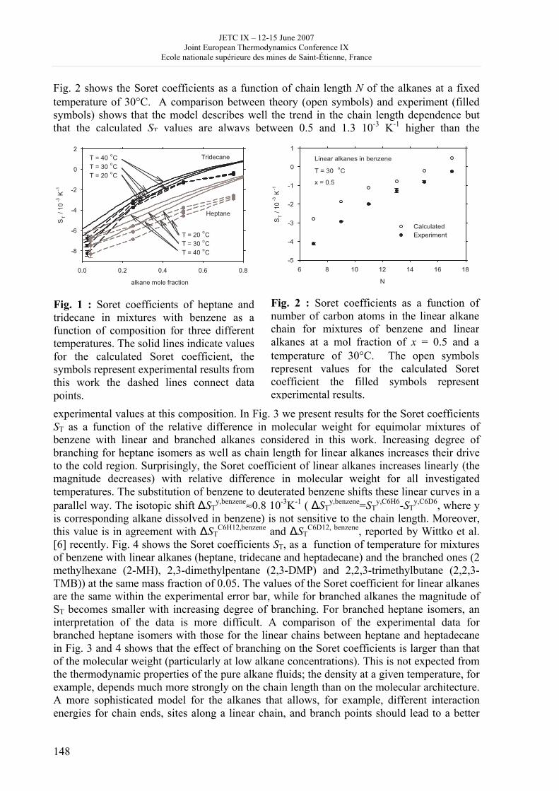
JETC IX – 12-15 June 2007 Joint European Thermodynamics Conference IX
Ecole nationale supérieure des mines de Saint-Étienne, France
148
Fig. 2 shows the Soret coefficients as a function of chain length N of the alkanes at a fixed temperature of 30°C. A comparison between theory (open symbols) and experiment (filled symbols) shows that the model describes well the trend in the chain length dependence but that the calculated ST values are always between 0.5 and 1.3 10-3 K-1 higher than the
experimental values at this composition. In Fig. 3 we present results for the Soret coefficients ST as a function of the relative difference in molecular weight for equimolar mixtures of benzene with linear and branched alkanes considered in this work. Increasing degree of branching for heptane isomers as well as chain length for linear alkanes increases their drive to the cold region. Surprisingly, the Soret coefficient of linear alkanes increases linearly (the magnitude decreases) with relative difference in molecular weight for all investigated temperatures. The substitution of benzene to deuterated benzene shifts these linear curves in a parallel way. The isotopic shift ΔST
y,benzene≈0.8 10-3K-1 ( ΔSTy,benzene=ST
y,C6H6-STy,C6D6, where y
is corresponding alkane dissolved in benzene) is not sensitive to the chain length. Moreover, this value is in agreement with ΔST
C6H12,benzene and ΔSTC6D12, benzene, reported by Wittko et al.
[6] recently. Fig. 4 shows the Soret coefficients ST, as a function of temperature for mixtures of benzene with linear alkanes (heptane, tridecane and heptadecane) and the branched ones (2 methylhexane (2-MH), 2,3-dimethylpentane (2,3-DMP) and 2,2,3-trimethylbutane (2,2,3-TMB)) at the same mass fraction of 0.05. The values of the Soret coefficient for linear alkanes are the same within the experimental error bar, while for branched alkanes the magnitude of ST becomes smaller with increasing degree of branching. For branched heptane isomers, an interpretation of the data is more difficult. A comparison of the experimental data for branched heptane isomers with those for the linear chains between heptane and heptadecane in Fig. 3 and 4 shows that the effect of branching on the Soret coefficients is larger than that of the molecular weight (particularly at low alkane concentrations). This is not expected from the thermodynamic properties of the pure alkane fluids; the density at a given temperature, for example, depends much more strongly on the chain length than on the molecular architecture. A more sophisticated model for the alkanes that allows, for example, different interaction energies for chain ends, sites along a linear chain, and branch points should lead to a better
Fig. 1 : Soret coefficients of heptane and tridecane in mixtures with benzene as a function of composition for three different temperatures. The solid lines indicate values for the calculated Soret coefficient, the symbols represent experimental results from this work the dashed lines connect data points.
Fig. 2 : Soret coefficients as a function of number of carbon atoms in the linear alkane chain for mixtures of benzene and linear alkanes at a mol fraction of x = 0.5 and a temperature of 30°C. The open symbols represent values for the calculated Soret coefficient the filled symbols represent experimental results.
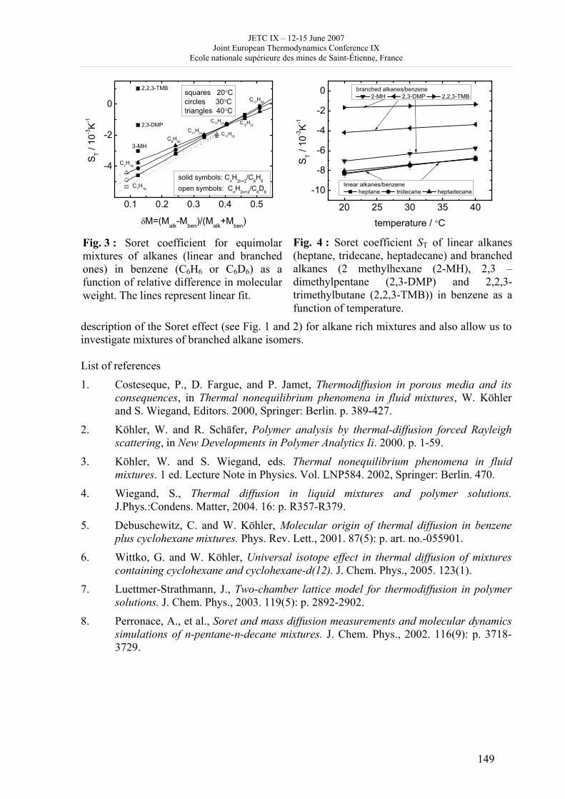
JETC IX – 12-15 June 2007 Joint European Thermodynamics Conference IX
Ecole nationale supérieure des mines de Saint-Étienne, France
149
description of the Soret effect (see Fig. 1 and 2) for alkane rich mixtures and also allow us to investigate mixtures of branched alkane isomers. List of references
1. Costeseque, P., D. Fargue, and P. Jamet, Thermodiffusion in porous media and its consequences, in Thermal nonequilibrium phenomena in fluid mixtures, W. Köhler and S. Wiegand, Editors. 2000, Springer: Berlin. p. 389-427.
2. Köhler, W. and R. Schäfer, Polymer analysis by thermal-diffusion forced Rayleigh scattering, in New Developments in Polymer Analytics Ii. 2000. p. 1-59.
3. Köhler, W. and S. Wiegand, eds. Thermal nonequilibrium phenomena in fluid mixtures. 1 ed. Lecture Note in Physics. Vol. LNP584. 2002, Springer: Berlin. 470.
4. Wiegand, S., Thermal diffusion in liquid mixtures and polymer solutions. J.Phys.:Condens. Matter, 2004. 16: p. R357-R379.
5. Debuschewitz, C. and W. Köhler, Molecular origin of thermal diffusion in benzene plus cyclohexane mixtures. Phys. Rev. Lett., 2001. 87(5): p. art. no.-055901.
6. Wittko, G. and W. Köhler, Universal isotope effect in thermal diffusion of mixtures containing cyclohexane and cyclohexane-d(12). J. Chem. Phys., 2005. 123(1).
7. Luettmer-Strathmann, J., Two-chamber lattice model for thermodiffusion in polymer solutions. J. Chem. Phys., 2003. 119(5): p. 2892-2902.
8. Perronace, A., et al., Soret and mass diffusion measurements and molecular dynamics simulations of n-pentane-n-decane mixtures. J. Chem. Phys., 2002. 116(9): p. 3718-3729.
Fig. 3 : Soret coefficient for equimolar mixtures of alkanes (linear and branched ones) in benzene (C6H6 or C6D6) as a function of relative difference in molecular weight. The lines represent linear fit.
Fig. 4 : Soret coefficient ST of linear alkanes (heptane, tridecane, heptadecane) and branched alkanes (2 methylhexane (2-MH), 2,3 – dimethylpentane (2,3-DMP) and 2,2,3-trimethylbutane (2,2,3-TMB)) in benzene as a function of temperature.
JETC IX – 12-15 June 2007 Joint European Thermodynamics Conference IX
Ecole nationale supérieure des mines de Saint-Étienne, France
150
The transition from single- to multi-cell natural convection of air in cavities with an aspect ratio of 20.
Michel PONS
CNRS-LIMSI, BP 133, 91403 Orsay Cedex, France
michel.pons @ limsi.fr Introduction Since the seminal work of Batchelor (1954), thermal convection in 2-D tall differentially-heated cavities (with aspect ratio A=H/L above 15) received great interest, probably because of its relevance in building engineering. Batchelor (1954) demonstrated that, sufficiently far away from the horizontal walls and when the Rayleigh number Ra is weak, the flow is 1-D, temperature T is a linear function of the horizontal position x (non-dimensional: 0≤x≤1/A) while vertical velocity is a cubic function: Vz=αL-1RaL(Ax–0.5)A(Ax2-x)/6; where α is the fluid thermal diffusivity and L is the cavity width. This is the conduction regime. It is well known that beyond a critical value of the Rayleigh number: RaL=βgL3ΔT(αν)-1, the flow undergoes a transition from single- to multi-cell pattern: secondary cells appear along the midline of the cavity (x=0.5/A), included in the external primary cell. Like the conduction regime, the transition regime leads to stable steady-states. (β is the thermal expansion coefficient, g the gravity acceleration, ΔT=Th-Tc the temperature difference between the two vertical walls, ν the fluid kinematic viscosity). That transition has been studied since the 60’s and still is, experimentally e.g. by Elder (1965), Lartigue et al. (2000) or Wright et al. (2006), numerically e.g. by Le Quéré (1990) or Zhao et al. (1997), and with linear stability analyses e.g. by Vest and Arpaci (1969) or Bergholz (1978). The present study develops a thermodynamic approach of that transition in cavities of fixed aspect ratio A = 20 filled with air at ambient temperature (300K, Pr = 0.71). The numerical model: thermodynamic Boussinesq equations The numerical model is based on the Boussinesq equations (Boussinesq, 1903), but slightly modified according to Spiegel and Veronis (1960). Following thermodynamic arguments, these authors keep in the heat equation two terms which are usually neglected: the work of pressure stress and the heat qv generated by viscous friction.
-1
2 ( )D DD D
v
Pp p
qT T PTt c T t c
ραρ
⎛ ⎞∂= ∇ + +⎜ ⎟∂⎝ ⎠
(1)
t stands for time, P for pressure, ρ for density, cp for heat capacity. They called the so-modified Boussinesq system, the thermodynamic Boussinesq equations. Indeed, these equations yield completely consistent thermodynamic balances especially with respect to the second law, when the usual Boussinesq equations do not. For non-dimensionalization, the reference quantities are: the cavity height H for distances, αL-1(ARaL)1/2 for velocities, ΔT for the difference T-T0, where T0=(Th+Tc)/2. Considering only the hydrostatic pressure gradient and that the average pressure is constant (obviously true at steady-state), the non-dimensionalized heat equation is:
21
pL L
gHu w w wx z cA ARa A ARa
θ θ θ βθ φ θτ
∂ ∂ ∂ Φ⎛ ⎞+ + = ∇ − + −⎜ ⎟∂ ∂ ∂ ⎝ ⎠ (2)
JETC IX – 12-15 June 2007 Joint European Thermodynamics Conference IX
Ecole nationale supérieure des mines de Saint-Étienne, France
151
where x, z, u, w, τ, and θ are the non-dimensional coordinates (horizontal, vertical), velocities (idem), time and temperature; φ=[βgHT0(cpΔT)-1] is the adiabatic temperature gradient [βgT0cp
-1] non-dimensionalized by the vertical temperature gradient in the problem [ΔT/H]; and Φ is the non-dimensional heat generated by viscous friction. The number [βgH/cp] appearing in the rightmost term is usually very small (of the order of 10-5 in this study). On the other hand, the term (-φw), which is practically the work of the pressure stress, can easily be of the order of unity and therefore should better not be neglected. * The equations are solved with a finite-difference second-order scheme on a staggered 128x512 grid, which is much finer than ever done before: Lee and Korpela (1983) used a 33x33 grid, and Le Quéré (1990) a 24x120. Moreover, our grid regular ensures correct resolution in the center of the cavity, there where the secondary cells take place. For more, see Pons and Le Quéré (2007). As the thermodynamic Boussinesq equations involve the parameters φ and βgH/cp, a given configuration cannot be described by the Rayleigh number only. Therefore two cavities with two given heights are considered herein: a small one, where the work of pressure stress is negligible (φ << 1), and a large one where it is not negligible (φ of the order of 1). The two cavities are described in Table 1, both are of human size, not of geophysics dimensions. The values of φ et ΔT given in Table 1 are those corresponding to RaL=5000. Values of RaL above 5000 are obtained just by increasing ΔT, so that φ is decreased proportionally.
Cavity H [m] φ_RaL=5000 ΔT_RaL=5000 [K] small large
0.808 2.032
0.01 0.4
0.789 0.0496
Table 1 : The two configurations investigated herein. Transition, heat fluxes and irreversibilities The first studies on that transition used stability analyses considering as base flow that defined by Batchelor (1954) and mentioned here above. The critical Rayleigh RaL lies between 5600 and 5700 (Vest and Arpaci, 1969;Bergholz, 1978). Purely numerical studies lead to larger values e.g. 6500 (Zhao et al., 1997). As all those evaluations are based on the usual Boussinesq equations, they can only apply to the present small cavity. In this short article, the thermodynamic analysis is based on two quantities. First, the Nusselt number, i.e. the ratio of the effective heat flux to that transferred in a purely conductive
system (fluid at rest): [ ( )110
dNu A x zθ−= ∂ ∂∫ ]. Second, the number of viscous irreversibility,
NIv. Indeed, in similarity with the Nusselt number, the irreversibilities are non-dimensionalized by the total entropy production of the purely conductive system. The numbers of viscous and conductive irreversibility are then given respectively by:
( ) ( ) ( ) ( ) 12 2 2102 2 . 1 d dIv
cavityN A u x u z w x w z T T x zφ θ −− ⎡ ⎤= ∂ ∂ + ∂ ∂ + ∂ ∂ + ∂ ∂ + Δ⎢ ⎥⎣ ⎦∫ and
( ) 2210. 1 d dIq
cavityN A T T x zθ θ −−= ∇ + Δ∫ , see (Pons and Le Quéré, 2005a, 2005b).
In the small cavity: Two secondary cells appear at the center of the cavity at RaL=5850, in agreement with the linear stability analyses. However, the thermodynamic analysis leads to a different threshold. The curves Nu and NIv vs. RaL, Figures 1 and 2, display knees at RaL=6100, i.e. when six secondary cells are formed in the cavity. If the relative increase of
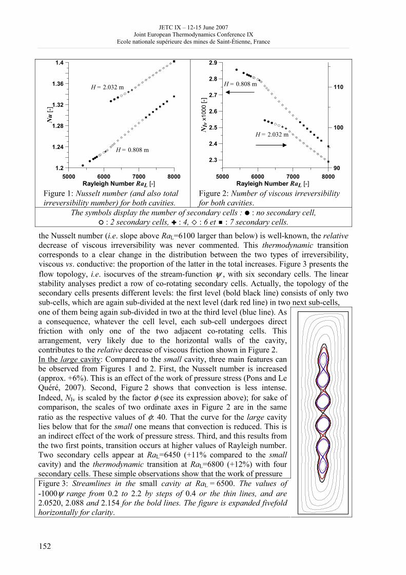
JETC IX – 12-15 June 2007 Joint European Thermodynamics Conference IX
Ecole nationale supérieure des mines de Saint-Étienne, France
152
5000 6000 7000 8000Rayleigh Number RaL [-]
1.2
1.24
1.28
1.32
1.36
1.4
Nu
[-]
H = 0.808 m
H = 2.032 m
Figure 1: Nusselt number (and also total irreversibility number) for both cavities.
5000 6000 7000 8000Rayleigh Number RaL [-]
2.3
2.4
2.5
2.6
2.7
2.8
2.9
NIv
x10
00 [-
]
90
100
110H = 0.808 m
H = 2.032 m
Figure 2: Number of viscous irreversibility for both cavities.
The symbols display the number of secondary cells : : no secondary cell, : 2 secondary cells, : 4, : 6 et : 7 secondary cells.
the Nusselt number (i.e. slope above RaL=6100 larger than below) is well-known, the relative decrease of viscous irreversibility was never commented. This thermodynamic transition corresponds to a clear change in the distribution between the two types of irreversibility, viscous vs. conductive: the proportion of the latter in the total increases. Figure 3 presents the flow topology, i.e. isocurves of the stream-function ψ , with six secondary cells. The linear stability analyses predict a row of co-rotating secondary cells. Actually, the topology of the secondary cells presents different levels: the first level (bold black line) consists of only two sub-cells, which are again sub-divided at the next level (dark red line) in two next sub-cells, one of them being again sub-divided in two at the third level (blue line). As a consequence, whatever the cell level, each sub-cell undergoes direct friction with only one of the two adjacent co-rotating cells. This arrangement, very likely due to the horizontal walls of the cavity, contributes to the relative decrease of viscous friction shown in Figure 2. In the large cavity: Compared to the small cavity, three main features can be observed from Figures 1 and 2. First, the Nusselt number is increased (approx. +6%). This is an effect of the work of pressure stress (Pons and Le Quéré, 2007). Second, Figure 2 shows that convection is less intense. Indeed, NIv is scaled by the factor φ (see its expression above); for sake of comparison, the scales of two ordinate axes in Figure 2 are in the same ratio as the respective values of φ: 40. That the curve for the large cavity lies below that for the small one means that convection is reduced. This is an indirect effect of the work of pressure stress. Third, and this results from the two first points, transition occurs at higher values of Rayleigh number. Two secondary cells appear at RaL=6450 (+11% compared to the small cavity) and the thermodynamic transition at RaL=6800 (+12%) with four secondary cells. These simple observations show that the work of pressure
Figure 3: Streamlines in the small cavity at RaL = 6500. The values of -1000ψ range from 0.2 to 2.2 by steps of 0.4 or the thin lines, and are 2.0520, 2.088 and 2.154 for the bold lines. The figure is expanded fivefold horizontally for clarity.
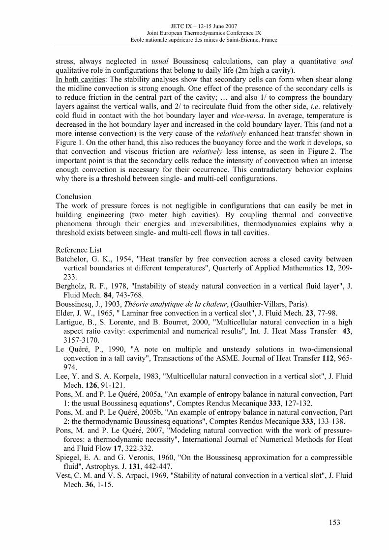
JETC IX – 12-15 June 2007 Joint European Thermodynamics Conference IX
Ecole nationale supérieure des mines de Saint-Étienne, France
153
stress, always neglected in usual Boussinesq calculations, can play a quantitative and qualitative role in configurations that belong to daily life (2m high a cavity). In both cavities: The stability analyses show that secondary cells can form when shear along the midline convection is strong enough. One effect of the presence of the secondary cells is to reduce friction in the central part of the cavity; … and also 1/ to compress the boundary layers against the vertical walls, and 2/ to recirculate fluid from the other side, i.e. relatively cold fluid in contact with the hot boundary layer and vice-versa. In average, temperature is decreased in the hot boundary layer and increased in the cold boundary layer. This (and not a more intense convection) is the very cause of the relatively enhanced heat transfer shown in Figure 1. On the other hand, this also reduces the buoyancy force and the work it develops, so that convection and viscous friction are relatively less intense, as seen in Figure 2. The important point is that the secondary cells reduce the intensity of convection when an intense enough convection is necessary for their occurrence. This contradictory behavior explains why there is a threshold between single- and multi-cell configurations. Conclusion The work of pressure forces is not negligible in configurations that can easily be met in building engineering (two meter high cavities). By coupling thermal and convective phenomena through their energies and irreversibilities, thermodynamics explains why a threshold exists between single- and multi-cell flows in tall cavities. Reference List Batchelor, G. K., 1954, "Heat transfer by free convection across a closed cavity between
vertical boundaries at different temperatures", Quarterly of Applied Mathematics 12, 209-233.
Bergholz, R. F., 1978, "Instability of steady natural convection in a vertical fluid layer", J. Fluid Mech. 84, 743-768.
Boussinesq, J., 1903, Théorie analytique de la chaleur, (Gauthier-Villars, Paris). Elder, J. W., 1965, " Laminar free convection in a vertical slot", J. Fluid Mech. 23, 77-98. Lartigue, B., S. Lorente, and B. Bourret, 2000, "Multicellular natural convection in a high
aspect ratio cavity: experimental and numerical results", Int. J. Heat Mass Transfer 43, 3157-3170.
Le Quéré, P., 1990, "A note on multiple and unsteady solutions in two-dimensional convection in a tall cavity", Transactions of the ASME. Journal of Heat Transfer 112, 965-974.
Lee, Y. and S. A. Korpela, 1983, "Multicellular natural convection in a vertical slot", J. Fluid Mech. 126, 91-121.
Pons, M. and P. Le Quéré, 2005a, "An example of entropy balance in natural convection, Part 1: the usual Boussinesq equations", Comptes Rendus Mecanique 333, 127-132.
Pons, M. and P. Le Quéré, 2005b, "An example of entropy balance in natural convection, Part 2: the thermodynamic Boussinesq equations", Comptes Rendus Mecanique 333, 133-138.
Pons, M. and P. Le Quéré, 2007, "Modeling natural convection with the work of pressure-forces: a thermodynamic necessity", International Journal of Numerical Methods for Heat and Fluid Flow 17, 322-332.
Spiegel, E. A. and G. Veronis, 1960, "On the Boussinesq approximation for a compressible fluid", Astrophys. J. 131, 442-447.
Vest, C. M. and V. S. Arpaci, 1969, "Stability of natural convection in a vertical slot", J. Fluid Mech. 36, 1-15.

JETC IX – 12-15 June 2007 Joint European Thermodynamics Conference IX
Ecole nationale supérieure des mines de Saint-Étienne, France
154
Wright, J. L., H. Jin, K. G. T. Hollands, and D. Naylor, 2006, "Flow visualization of natural convection in a tall, air-filled vertical cavity", Int. J. Heat Mass Transfer 49, 889-904.
Zhao, Y., D. Curcija, and W. P. Goss, 1997, "Prediction of the multicellular flow regime of natural convection in fenestration glazing cavities", ASHRAE Transactions 103, 1-12.
Keywords : Free convection, numerical model, thermodynamics, irreversibilities.
The numerical calculations were done on the NEC-SX8 of CNRS-IDRIS, Orsay.
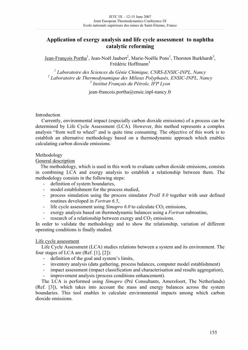
JETC IX – 12-15 June 2007 Joint European Thermodynamics Conference IX
Ecole nationale supérieure des mines de Saint-Étienne, France
155
Application of exergy analysis and life cycle assessment to naphtha catalytic reforming
Jean-François Portha1, Jean-Noël Jaubert2, Marie-Noëlle Pons1, Thorsten Burkhardt3, Frédéric Hoffmann3
1 Laboratoire des Sciences du Génie Chimique, CNRS-ENSIC-INPL, Nancy 2 Laboratoire de Thermodynamique des Milieux Polyphasés, ENSIC-INPL, Nancy
3 Institut Français du Pétrole, IFP Lyon
[email protected] Introduction
Currently, environmental impact (especially carbon dioxide emissions) of a process can be determined by Life Cycle Assessment (LCA). However, this method represents a complex analysis “from well to wheel” and is quite time consuming. The objective of this work is to establish an alternative methodology based on a thermodynamic approach which enables calculating carbon dioxide emissions.
Methodology General description
The methodology, which is used in this work to evaluate carbon dioxide emissions, consists in combining LCA and exergy analysis to establish a relationship between them. The methodology consists in the following steps:
- definition of system boundaries, - model establishment for the process studied, - process simulation using the process simulator ProII 8.0 together with user defined
routines developed in Fortran 6.5, - life cycle assessment using Simapro 6.0 to calculate CO2 emissions, - exergy analysis based on thermodynamic balances using a Fortran subroutine, - research of a relationship between exergy and CO2 emissions.
In order to validate the methodology and to show the relationship, variation of different operating conditions is finally studied. Life cycle assessment
Life Cycle Assessment (LCA) studies relations between a system and its environment. The four stages of LCA are (Ref. [1], [2]):
- definition of the goal and system’s limits, - inventory analysis (data gathering, process balances, computer model establishment) - impact assessment (impact classification and characterisation and results aggregation), - improvement analysis (process conditions enhancement).
The LCA is performed using Simapro (Pré Consultants, Amersfoort, The Netherlands) (Ref. [3]), which takes into account the mass and energy balances across the system boundaries. This tool enables to calculate environmental impacts among which carbon dioxide emissions.
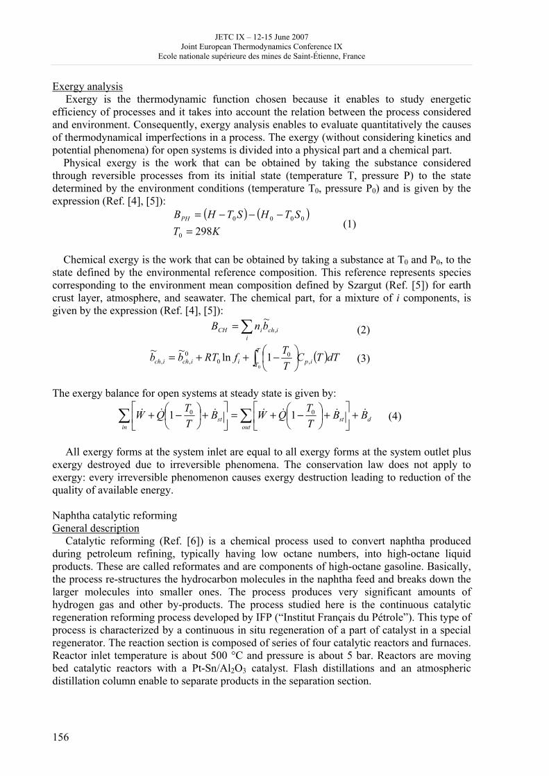
JETC IX – 12-15 June 2007 Joint European Thermodynamics Conference IX
Ecole nationale supérieure des mines de Saint-Étienne, France
156
Exergy analysis Exergy is the thermodynamic function chosen because it enables to study energetic
efficiency of processes and it takes into account the relation between the process considered and environment. Consequently, exergy analysis enables to evaluate quantitatively the causes of thermodynamical imperfections in a process. The exergy (without considering kinetics and potential phenomena) for open systems is divided into a physical part and a chemical part.
Physical exergy is the work that can be obtained by taking the substance considered through reversible processes from its initial state (temperature T, pressure P) to the state determined by the environment conditions (temperature T0, pressure P0) and is given by the expression (Ref. [4], [5]):
( ) ( )KT
STHSTHBPH
2980
0000
=−−−=
(1)
Chemical exergy is the work that can be obtained by taking a substance at T0 and P0, to the
state defined by the environmental reference composition. This reference represents species corresponding to the environment mean composition defined by Szargut (Ref. [5]) for earth crust layer, atmosphere, and seawater. The chemical part, for a mixture of i components, is given by the expression (Ref. [4], [5]):
∑=i
ichiCH bnB ,~ (2)
( )dTTCTTfRTbb ip
T
Tiichich ,0
00
,,0
1ln~~∫ ⎟
⎠⎞
⎜⎝⎛ −++= (3)
The exergy balance for open systems at steady state is given by:
dout
stin
st BBTTQWB
TTQW &&&&&&& +⎥
⎦
⎤⎢⎣
⎡ +⎟⎠⎞
⎜⎝⎛ −+=⎥
⎦
⎤⎢⎣
⎡ +⎟⎠⎞
⎜⎝⎛ −+ ∑∑ 00 11 (4)
All exergy forms at the system inlet are equal to all exergy forms at the system outlet plus
exergy destroyed due to irreversible phenomena. The conservation law does not apply to exergy: every irreversible phenomenon causes exergy destruction leading to reduction of the quality of available energy. Naphtha catalytic reforming General description
Catalytic reforming (Ref. [6]) is a chemical process used to convert naphtha produced during petroleum refining, typically having low octane numbers, into high-octane liquid products. These are called reformates and are components of high-octane gasoline. Basically, the process re-structures the hydrocarbon molecules in the naphtha feed and breaks down the larger molecules into smaller ones. The process produces very significant amounts of hydrogen gas and other by-products. The process studied here is the continuous catalytic regeneration reforming process developed by IFP (“Institut Français du Pétrole”). This type of process is characterized by a continuous in situ regeneration of a part of catalyst in a special regenerator. The reaction section is composed of series of four catalytic reactors and furnaces. Reactor inlet temperature is about 500 °C and pressure is about 5 bar. Reactors are moving bed catalytic reactors with a Pt-Sn/Al2O3 catalyst. Flash distillations and an atmospheric distillation column enable to separate products in the separation section.
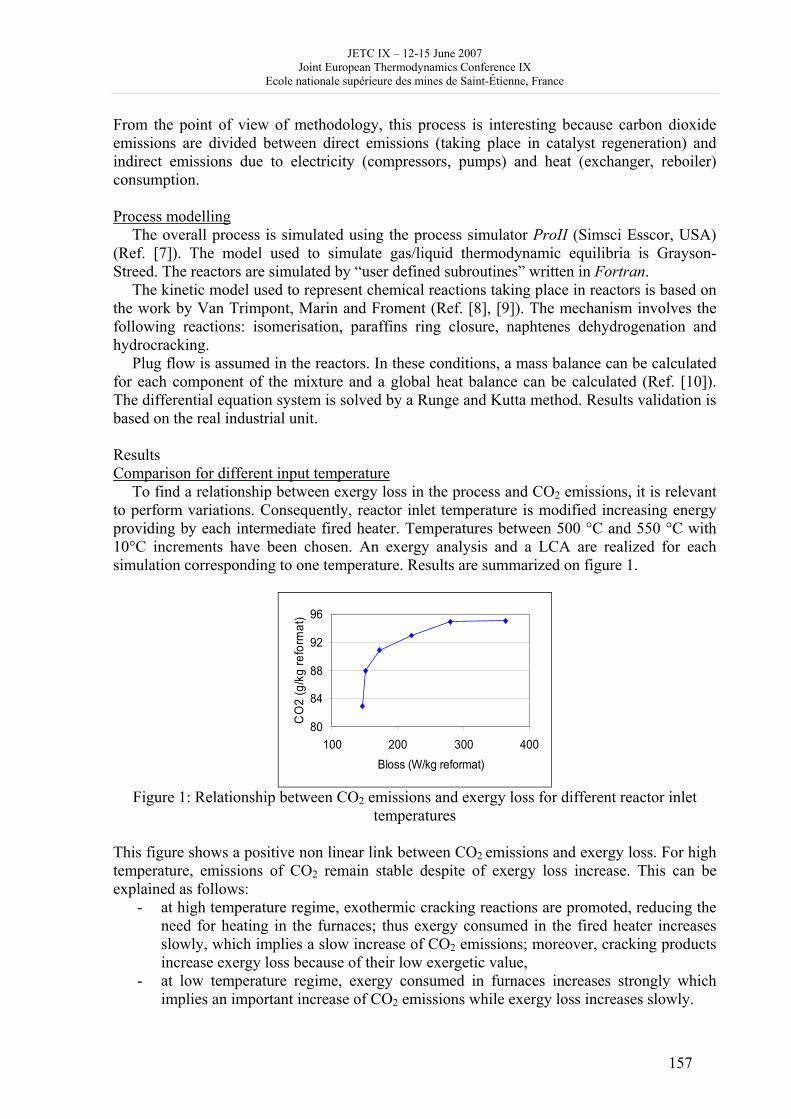
JETC IX – 12-15 June 2007 Joint European Thermodynamics Conference IX
Ecole nationale supérieure des mines de Saint-Étienne, France
157
From the point of view of methodology, this process is interesting because carbon dioxide emissions are divided between direct emissions (taking place in catalyst regeneration) and indirect emissions due to electricity (compressors, pumps) and heat (exchanger, reboiler) consumption. Process modelling
The overall process is simulated using the process simulator ProII (Simsci Esscor, USA) (Ref. [7]). The model used to simulate gas/liquid thermodynamic equilibria is Grayson-Streed. The reactors are simulated by “user defined subroutines” written in Fortran.
The kinetic model used to represent chemical reactions taking place in reactors is based on the work by Van Trimpont, Marin and Froment (Ref. [8], [9]). The mechanism involves the following reactions: isomerisation, paraffins ring closure, naphtenes dehydrogenation and hydrocracking.
Plug flow is assumed in the reactors. In these conditions, a mass balance can be calculated for each component of the mixture and a global heat balance can be calculated (Ref. [10]). The differential equation system is solved by a Runge and Kutta method. Results validation is based on the real industrial unit.
Results Comparison for different input temperature
To find a relationship between exergy loss in the process and CO2 emissions, it is relevant to perform variations. Consequently, reactor inlet temperature is modified increasing energy providing by each intermediate fired heater. Temperatures between 500 °C and 550 °C with 10°C increments have been chosen. An exergy analysis and a LCA are realized for each simulation corresponding to one temperature. Results are summarized on figure 1.
80
84
88
92
96
100 200 300 400Bloss (W/kg reformat)
CO
2 (g
/kg
refo
rmat
)
Figure 1: Relationship between CO2 emissions and exergy loss for different reactor inlet
temperatures This figure shows a positive non linear link between CO2 emissions and exergy loss. For high temperature, emissions of CO2 remain stable despite of exergy loss increase. This can be explained as follows:
- at high temperature regime, exothermic cracking reactions are promoted, reducing the need for heating in the furnaces; thus exergy consumed in the fired heater increases slowly, which implies a slow increase of CO2 emissions; moreover, cracking products increase exergy loss because of their low exergetic value,
- at low temperature regime, exergy consumed in furnaces increases strongly which implies an important increase of CO2 emissions while exergy loss increases slowly.
JETC IX – 12-15 June 2007 Joint European Thermodynamics Conference IX
Ecole nationale supérieure des mines de Saint-Étienne, France
158
Restrictions For the time being, our methodology suffers of some limitations. Indeed, exergy analysis is
carried out for the process only, without considering exergy destruction due to heat production and electricity production. Consequently, results will be improved by taking into account exergy destruction in furnaces (development of a model for furnaces) and exergy destruction in power plants. Moreover this model could give information about CO2 production from fuel combustion and this result could be compared to LCA results.
Conclusion
LCA analysis and exergy analysis are tools providing solutions to analyze processes and to determine environmental impact. With these tools a relationship has been establish between exergy loss and CO2 emissions in this work. The first results for the chosen process and the chosen parameter variation (reactor inlet temperature) show that the more exergy is destroyed, the higher the carbon dioxide emissions are. This result has already been observed in a previous work without taking into account chemical exergy (Ref. [11]).
The aim of this work was to establish a methodology based on a thermodynamic analysis without using Life Cycle Assessment. The non linear link between carbon dioxide emissions and exergy destruction has to be confirmed and quantified in future investigations. To achieve these objectives, others simulations will be carried out with additional operating conditions. If these results are confirmed, the methodology will be generalised to other processes.
References [1] J. Chevalier, Elaboration d’un protocole d’analyse de cycle de vie des procédés. Phd Dissertation, Institut National des Sciences Appliquées de Lyon, 1999. [2] R.L. Cornelissen, Thermodynamics and sustainable development, the use of exergy analysis and the reduction of irreversibility. Phd Dissertation, Enschede, the Netherlands, 1997. [3] Pré Consultants, Simapro 6, The Netherlands, 2004. [4] T.J. Kotas, The exergy method of thermal plant analysis. Krieger Publishing Company, Krieger Drive, Florida, 1995. [5] J. Szargut, Exergy method, technical and ecological applications. WIT Press, 2005. [6] R.A. Meyers, Handbook of petroleum refining processes. Second Editions, McGraw-Hill, 1996. [7] Simsci-Esscor, Pro II 7.0, United States of America, 2004. [8] G.B. Marin, G.F. Froment, Reforming of C6 hydrocarbons on a Pt/Al2O3 catalyst. Chemical Engineering Science, Vol. 37, No. 5, p. 759-773, 1981. [9] P.A. Van Trimpont, G.B. Marin, G.F. Froment, Reforming of C7 hydrocarbons on a sulfied commercial Pt/Al2O3 catalyst. Industrial Engineering Chemical Research, Vol. 27, p. 51-57, 1988. [10] J. Villermaux, Génie de la réaction chimique, conception et fonctionnement des réacteurs. Tec&Doc, Lavoisier, Paris, 1985. [11] J.F. Portha, A. Archane, M.N. Pons, J.N. Jaubert, T. Burkhardt, F. Hoffmann, Application of exergy analysis and life cycle assessment to the oil industry, Proceedings ECOS 2006.
JETC IX – 12-15 June 2007 Joint European Thermodynamics Conference IX
Ecole nationale supérieure des mines de Saint-Étienne, France
159
Entropic skins geometry and dynamics of turbulent reactive fronts
Diogo Queiros-Conde1 and Michel Feidt2 1ENSTA, Unité Chimie et Procédés, 32 Bb Victor, 75015 Paris
2LEMTA, ENSEM-INPL, 2 Av. de la Forêt de Haye, F-54504 Vandoeuvre lès Nancy
[email protected] Introduction Our aim in this presentation is to propose a geometrical way to study dynamics of turbulent reactive fronts by using the concept of scale entropy and a diffusion equation ruling this quantity established by the introduction of a new quantity in physics called “scale diffusivity” which characterizes how information concerning the multi-scale structure propagates through scale-space and how it unifies the system giving it a kind of “structural viscosity” in scale-space. This description derives from a more general framework called “entropic skins geometry” introduced to deal with the phenomenon of intermittency in turbulence and turbulent reactive systems. After a recall of the phenomenon of turbulent combustion, we will present our geometrical approach and then we will show how it can be applied in the field of turbulent combustion and, more generally, to the field of turbulent reactive fronts. Our long-term aim through this work is to establish links between this topological approach with classical quantities of non-equilibrium thermodynamics. We also think that such a way can help to visualize some traditional thermodynamical quantities. The interaction turbulence-reactive front: the turbulent velocity The study of turbulent combustion has started with the work by Mallard and Le Chatelier (1883) at the end of nineteenth century (realized at Ecole des mines de St-Etienne). The fundamental problem in turbulent combustion is to characterize how scales of turbulence influence the flame structure (front wrinkling, front thickening, quenching) and how this one, by heat production and hydrodynamical instabilities, influence the characteristics of turbulence. Thanks to the development of laser visualisation techniques, the multi-scale structure of turbulent flames has been revealed leading to the application to this field of fractal theory without real success to describe turbulent flames dynamics. A more complex multi-scale geometry is needed. The figure 1 represents an example of turbulent flame obtained by laser tomography [1]. The main effect of turbulence is to wrinkle the flame front and, if the flow contains scales smaller than the flame thickness, to thicken the front. In the “flamelet” regime, the problem is simplified by the fact that chemical time and flame thickness are much smaller than the time and spatial scales characterizing the turbulence cascade. Our study concerns this case since our main aim is to understand turbulence-combustion interaction. This is the case for the flame given at figure 1. The turbulent velocity UT results from the wrinkling process of the whole scale range of the turbulence cascade which can be defined by its turbulent intensity U’. The chemical part is defined by the thickness of the front δ and the laminar velocity UL. The flame surface is increased by the effect of wrinkling and leads to a turbulent surface ST which has a multi-scale structure. There is a direct relation between velocities and surfaces through the relation UT/UL=ST/SL where SL is the projected flame surface perpendicular to the mean direction given by UT and which also corresponds to the
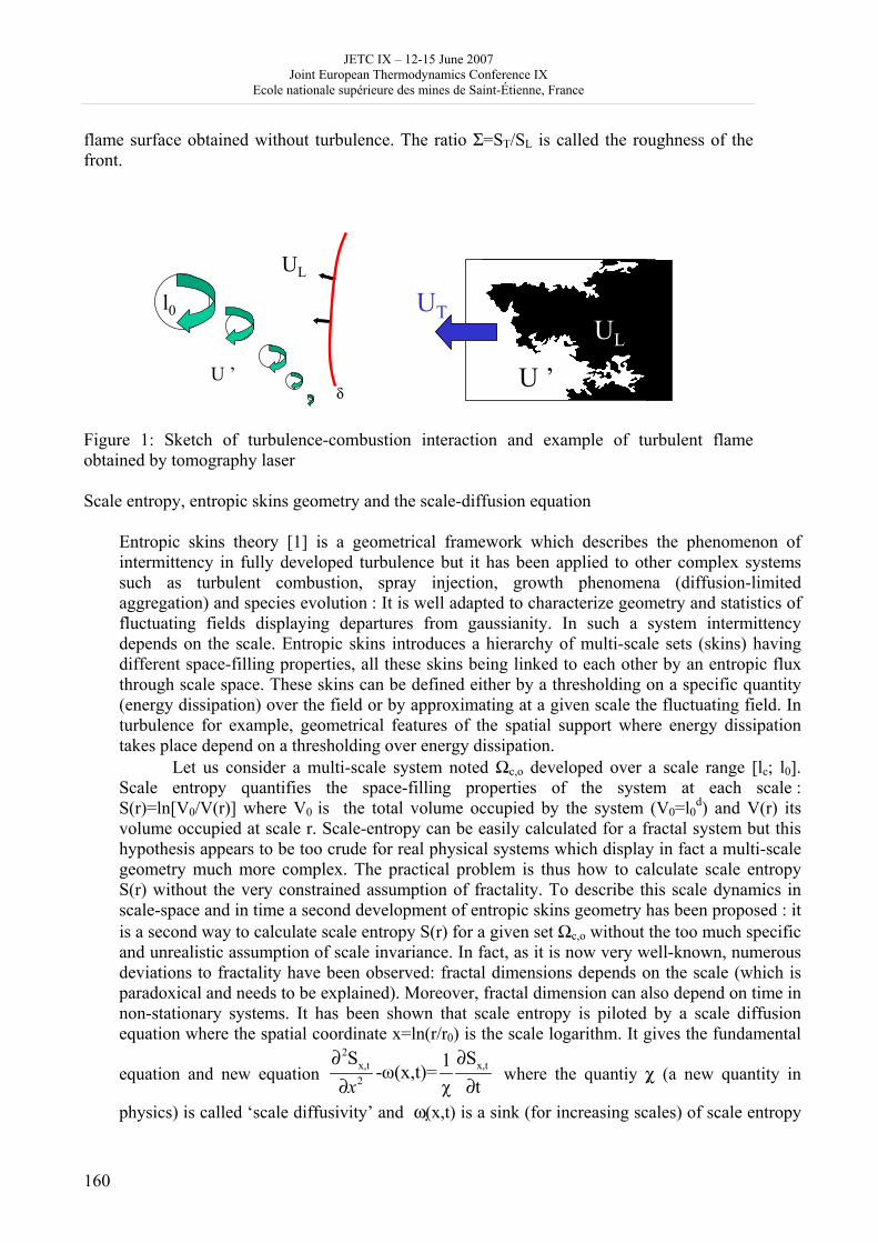
JETC IX – 12-15 June 2007 Joint European Thermodynamics Conference IX
Ecole nationale supérieure des mines de Saint-Étienne, France
160
flame surface obtained without turbulence. The ratio Σ=ST/SL is called the roughness of the front.
U ’
UL
l0
δ U ’
UL
UT
Figure 1: Sketch of turbulence-combustion interaction and example of turbulent flame obtained by tomography laser Scale entropy, entropic skins geometry and the scale-diffusion equation
Entropic skins theory [1] is a geometrical framework which describes the phenomenon of intermittency in fully developed turbulence but it has been applied to other complex systems such as turbulent combustion, spray injection, growth phenomena (diffusion-limited aggregation) and species evolution : It is well adapted to characterize geometry and statistics of fluctuating fields displaying departures from gaussianity. In such a system intermittency depends on the scale. Entropic skins introduces a hierarchy of multi-scale sets (skins) having different space-filling properties, all these skins being linked to each other by an entropic flux through scale space. These skins can be defined either by a thresholding on a specific quantity (energy dissipation) over the field or by approximating at a given scale the fluctuating field. In turbulence for example, geometrical features of the spatial support where energy dissipation takes place depend on a thresholding over energy dissipation.
Let us consider a multi-scale system noted Ωc,o developed over a scale range [lc; l0]. Scale entropy quantifies the space-filling properties of the system at each scale : S(r)=ln[V0/V(r)] where V0 is the total volume occupied by the system (V0=l0
d) and V(r) its volume occupied at scale r. Scale-entropy can be easily calculated for a fractal system but this hypothesis appears to be too crude for real physical systems which display in fact a multi-scale geometry much more complex. The practical problem is thus how to calculate scale entropy S(r) without the very constrained assumption of fractality. To describe this scale dynamics in scale-space and in time a second development of entropic skins geometry has been proposed : it is a second way to calculate scale entropy S(r) for a given set Ωc,o without the too much specific and unrealistic assumption of scale invariance. In fact, as it is now very well-known, numerous deviations to fractality have been observed: fractal dimensions depends on the scale (which is paradoxical and needs to be explained). Moreover, fractal dimension can also depend on time in non-stationary systems. It has been shown that scale entropy is piloted by a scale diffusion equation where the spatial coordinate x=ln(r/r0) is the scale logarithm. It gives the fundamental
equation and new equation 2
x,t x,t2
S S1-ω(x,t)=χ tx
∂ ∂∂ ∂
where the quantiy χ (a new quantity in
physics) is called ‘scale diffusivity’ and ω( x,t) is a sink (for increasing scales) of scale entropy
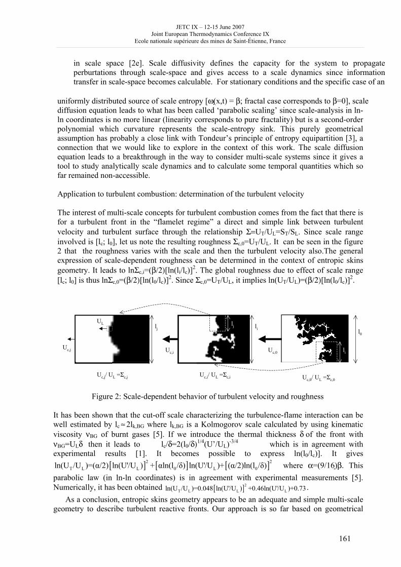
JETC IX – 12-15 June 2007 Joint European Thermodynamics Conference IX
Ecole nationale supérieure des mines de Saint-Étienne, France
161
in scale space [2e]. Scale diffusivity defines the capacity for the system to propagate perburtations through scale-space and gives access to a scale dynamics since information transfer in scale-space becomes calculable. For stationary conditions and the specific case of an
uniformly distributed source of scale entropy [ω( x,t) = β; fractal case corresponds to β=0], scale diffusion equation leads to what has been called ‘parabolic scaling’ since scale-analysis in ln-ln coordinates is no more linear (linearity corresponds to pure fractality) but is a second-order polynomial which curvature represents the scale-entropy sink. This purely geometrical assumption has probably a close link with Tondeur’s principle of entropy equipartition [3], a connection that we would like to explore in the context of this work. The scale diffusion equation leads to a breakthrough in the way to consider multi-scale systems since it gives a tool to study analytically scale dynamics and to calculate some temporal quantities which so far remained non-accessible. Application to turbulent combustion: determination of the turbulent velocity The interest of multi-scale concepts for turbulent combustion comes from the fact that there is for a turbulent front in the “flamelet regime” a direct and simple link between turbulent velocity and turbulent surface through the relationship Σ=UT/UL=ST/SL. Since scale range involved is [lc; l0], let us note the resulting roughness Σc,0=UT/UL. It can be seen in the figure 2 that the roughness varies with the scale and then the turbulent velocity also.The general expression of scale-dependent roughness can be determined in the context of entropic skins geometry. It leads to lnΣc,i=(β/2)[ln(li/lc)]2. The global roughness due to effect of scale range [lc; l0] is thus lnΣc,0=(β/2)[ln(l0/lc)]2. Since Σc,0=UT/UL, it implies ln(UT/UL)=(β/2)[ln(l0/lc)]2.
UL
l0
li
ljlj li
Uc,i/ UL =Σc,i
Uc,i Uc,0Uc,j
Uc,j/ UL =Σc,j Uc,0/ UL =Σc,0
Figure 2: Scale-dependent behavior of turbulent velocity and roughness It has been shown that the cut-off scale characterizing the turbulence-flame interaction can be well estimated by lc ≈ 2lk,BG where lk,BG is a Kolmogorov scale calculated by using kinematic viscosity νBG of burnt gases [5]. If we introduce the thermal thickness δ of the front with νBG=ULδ then it leads to lc/δ=2(l0/δ)1/4(U’/UL)-3/4 which is in agreement with experimental results [1]. It becomes possible to express ln(l0/lc)]. It gives
[ ] [ ] [ ]2 2T L L 0 L 0ln(U /U )=(α/2) ln(U'/U ) + αln(l /δ) ln(U'/U )+ (α/2)ln(l /δ) where α=(9/16)β. This
parabolic law (in ln-ln coordinates) is in agreement with experimental measurements [5]. Numerically, it has been obtained [ ]2
T L L Lln(U /U )=0.048 ln(U'/U ) +0.46ln(U'/U )+0.73. As a conclusion, entropic skins geometry appears to be an adequate and simple multi-scale
geometry to describe turbulent reactive fronts. Our approach is so far based on geometrical
JETC IX – 12-15 June 2007 Joint European Thermodynamics Conference IX
Ecole nationale supérieure des mines de Saint-Étienne, France
162
arguments but recent developments showed that it could be linked to thermodynamical arguments coming from specific optimization methods in thermodynamics [6].We hope to develop these aspects in future work.
References: [1] About Entropic Skins Geometry: D. Queiros-Conde: (a) "Geometry of intermittency in
fully-developed turbulence", C. R. Acad. Sci.", t. 327 série II b, 1385 (1999). (b) "Entropic skins model for fully-developed turbulence ", C. R. Acad. Sci, t. 328, série IIb , 541 (2000). (c) " Principle of flux entropy conservation in species evolution", C. R. Acad. Sci, série IIa 330, 445 (2000). (d) "Internal symmetry in the multifractal spectrum of fully developed turbulence", Phys. Rev. E, 64 015301(R) (2001). (e) "A diffusion equation to describe scale- and time-dependent dimensions of turbulent interfaces", Proc. R. Soc. Lond. A 459, 3043 (2003). (f) “Entropic Skins Dynamics for intermittent and multi-scale systems”, Habilitation à Diriger des Recherches (Nancy 1), 2006.
[2] D. Queiros-Conde, PhD Thesis, University of Provence, Marseille, France, 1996. See also A. Pocheau and D. Queiros-Conde, Phys. Rev. Lett. 76 (1996) 3352.
[3] D. Tondeur and E. Kvaalen, Ind. & Eng. Chem. Res., 26 (1987)50. [4] P.D. Ronney, B.D. Haslam, and N.O. Rhys., Phys. Rev. Letters, 74 (1995)3804. ; S. Shy,
Ronney P.D., Buckley S.G. and Yakhot V., Twenty-Fourth International Symposium on Combustion, Combustion, Institute, 1992, p. 543.
[5] D. Queiros-Conde an M. Feidt, Scientific Bulletin of the Politehnica, University of Timisoara, Transactions on mechanics, Fascicola 1, 2006.
[6] M. Feidt, Thermodynamique et optimisation énergétique des systèmes et des procédés, Ed. Tec & Doc, Paris, France, 1996.
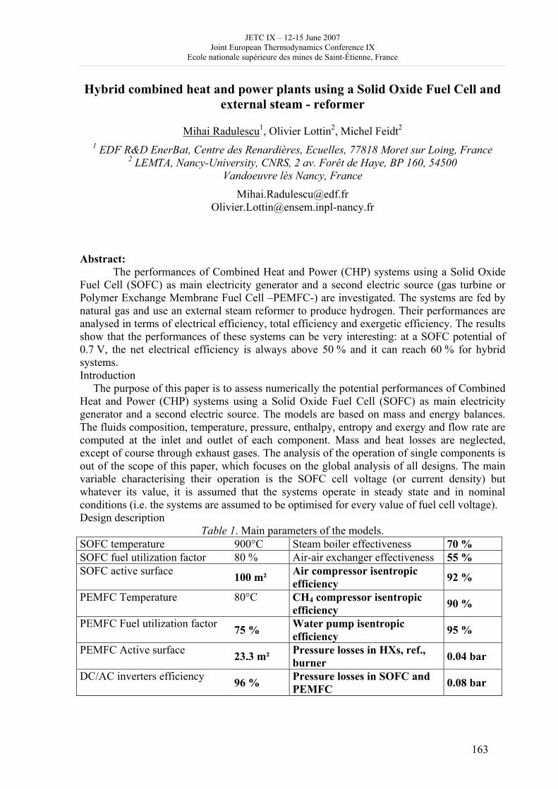
JETC IX – 12-15 June 2007 Joint European Thermodynamics Conference IX
Ecole nationale supérieure des mines de Saint-Étienne, France
163
Hybrid combined heat and power plants using a Solid Oxide Fuel Cell and external steam - reformer
Mihai Radulescu1, Olivier Lottin2, Michel Feidt2 1 EDF R&D EnerBat, Centre des Renardières, Ecuelles, 77818 Moret sur Loing, France
2 LEMTA, Nancy-University, CNRS, 2 av. Forêt de Haye, BP 160, 54500 Vandoeuvre lès Nancy, France
[email protected] [email protected]
Abstract:
The performances of Combined Heat and Power (CHP) systems using a Solid Oxide Fuel Cell (SOFC) as main electricity generator and a second electric source (gas turbine or Polymer Exchange Membrane Fuel Cell –PEMFC-) are investigated. The systems are fed by natural gas and use an external steam reformer to produce hydrogen. Their performances are analysed in terms of electrical efficiency, total efficiency and exergetic efficiency. The results show that the performances of these systems can be very interesting: at a SOFC potential of 0.7 V, the net electrical efficiency is always above 50 % and it can reach 60 % for hybrid systems. Introduction
The purpose of this paper is to assess numerically the potential performances of Combined Heat and Power (CHP) systems using a Solid Oxide Fuel Cell (SOFC) as main electricity generator and a second electric source. The models are based on mass and energy balances. The fluids composition, temperature, pressure, enthalpy, entropy and exergy and flow rate are computed at the inlet and outlet of each component. Mass and heat losses are neglected, except of course through exhaust gases. The analysis of the operation of single components is out of the scope of this paper, which focuses on the global analysis of all designs. The main variable characterising their operation is the SOFC cell voltage (or current density) but whatever its value, it is assumed that the systems operate in steady state and in nominal conditions (i.e. the systems are assumed to be optimised for every value of fuel cell voltage). Design description
Table 1. Main parameters of the models. SOFC temperature 900°C Steam boiler effectiveness 70 % SOFC fuel utilization factor 80 % Air-air exchanger effectiveness 55 % SOFC active surface 100 m² Air compressor isentropic
efficiency 92 %
PEMFC Temperature 80°C CH4 compressor isentropic efficiency 90 %
PEMFC Fuel utilization factor 75 % Water pump isentropic efficiency 95 %
PEMFC Active surface 23.3 m² Pressure losses in HXs, ref., burner 0.04 bar
DC/AC inverters efficiency 96 % Pressure losses in SOFC and PEMFC 0.08 bar
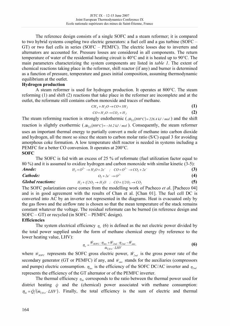
JETC IX – 12-15 June 2007 Joint European Thermodynamics Conference IX
Ecole nationale supérieure des mines de Saint-Étienne, France
164
The reference design consists of a single SOFC and a steam reformer; it is compared to two hybrid systems coupling two electric generators: a fuel cell and a gas turbine (SOFC – GT) or two fuel cells in series (SOFC – PEMFC). The electric losses due to inverters and alternators are accounted for. Pressure losses are considered in all components. The return temperature of water of the residential heating circuit is 40°C and it is heated up to 90°C. The main parameters characterizing the system components are listed in table 1. The extent of chemical reactions taking place in the reformer, shift reactor (if any) and burner is determined as a function of pressure, temperature and gases initial composition, assuming thermodynamic equilibrium at the outlet. Hydrogen production
A steam reformer is used for hydrogen production. It operates at 800°C. The steam reforming (1) and shift (2) reactions that take place in the reformer are incomplete and at the outlet, the reformate still contains carbon monoxide and traces of methane. 224 H3COOHCH +→+ (1) 222 HCOOHCO +→+ (2) The steam reforming reaction is strongly endothermic ( ( ) ( ) mol/kJ4.226C800h 1 =°Δ ) and the shift reaction is slightly exothermic ( ( ) ( ) mol/kJ2.34C800h 2 −=°Δ ). Consequently, the steam reformer uses an important thermal energy to partially convert a mole of methane into carbon dioxide and hydrogen, all the more so since the steam to carbon molar ratio (S/C) equal 3 for avoiding amorphous coke formation. A low temperature shift reactor is needed in systems including a PEMFC for a better CO conversion. It operates at 200°C. SOFC
The SOFC is fed with an excess of 25 % of reformate (fuel utilization factor equal to 80 %) and it is assumed to oxidize hydrogen and carbon monoxide with similar kinetic (3-5): Anode: −−−− +→++→+ e2COOCO;e2OHOH 2
22
22 (3)
Cathode: −− →+ 22 Oe2O (4)
Global reactions: 22222 COO21CO;OHO21H →+→+ (5) The SOFC polarization curve comes from the modelling work of Pacheco et al. [Pacheco 04] and is in good agreement with the results of Chan et al. [Chan 01]. The fuel cell DC is converted into AC by an inverter not represented in the diagrams. Heat is evacuated only by the gas flows and the airflow rate is chosen so that the mean temperature of the stack remains constant whatever the voltage. The residual reformate can be burned (in reference design and SOFC – GT) or recycled (in SOFC – PEMFC design). Efficiencies
The system electrical efficiency eη (6) is defined as the net electric power divided by the total power supplied under the form of methane chemical energy (by reference to the lower heating value, LHV):
LHVmWWW
4CH
auxnd2nd2invSOFCe ⋅
−⋅+⋅=
&
&&& ηηη (6)
where SOFCW& represents the SOFC gross electric power, nd2W& is the gross power rate of the secondary generator (GT or PEMFC) if any, and auxW& stands for the auxiliaries (compressors and pumps) electric consumption. invη is the efficiency of the SOFC DC/AC inverter and nd2η represents the efficiency of the GT alternator or of the PEMFC inverter.
The thermal efficiency thη corresponds to the ratio between the thermal power used for district heating Q& and the (chemical) power associated with methane consumption:
( )LHVmQ 4CHth ⋅= &&η . Finally, the total efficiency is the sum of electric and thermal
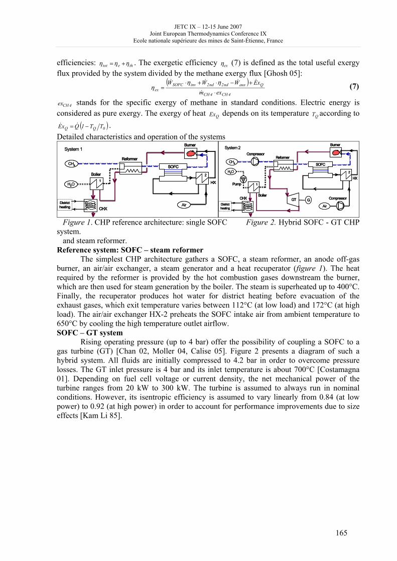
JETC IX – 12-15 June 2007 Joint European Thermodynamics Conference IX
Ecole nationale supérieure des mines de Saint-Étienne, France
165
efficiencies: thetot ηηη += . The exergetic efficiency exη (7) is defined as the total useful exergy flux provided by the system divided by the methane exergy flux [Ghosh 05]: ( )
4CH4CH
Qauxnd2nd2invSOFCex exm
xEWWW⋅
+−⋅+⋅=
&
&&&& ηηη (7)
4CHex stands for the specific exergy of methane in standard conditions. Electric energy is considered as pure exergy. The exergy of heat QEx depends on its temperature QT according to
( )0QQ TT1QxE −= && . Detailed characteristics and operation of the systems
System 1
Air
H2O
CH4
Reformer
SOFC
Burner
Boiler
HX
Districtheating
12
CHX
System 1
Air
H2O
CH4
Reformer
SOFC
Burner
Boiler
HX
Districtheating
12
CHX
System 2
Pump
CompressorGGTAir
H2O
CH4
Reformer
SOFC
Burner
Boiler
HX
Districtheating
CHX
1
2
CompressorSystem 2
Pump
CompressorGGTAir
H2O
CH4
Reformer
SOFC
Burner
Boiler
HX
Districtheating
CHX
1
2
Compressor
Figure 1. CHP reference architecture: single SOFC Figure 2. Hybrid SOFC - GT CHP
system. and steam reformer.
Reference system: SOFC – steam reformer The simplest CHP architecture gathers a SOFC, a steam reformer, an anode off-gas
burner, an air/air exchanger, a steam generator and a heat recuperator (figure 1). The heat required by the reformer is provided by the hot combustion gases downstream the burner, which are then used for steam generation by the boiler. The steam is superheated up to 400°C. Finally, the recuperator produces hot water for district heating before evacuation of the exhaust gases, which exit temperature varies between 112°C (at low load) and 172°C (at high load). The air/air exchanger HX-2 preheats the SOFC intake air from ambient temperature to 650°C by cooling the high temperature outlet airflow. SOFC – GT system
Rising operating pressure (up to 4 bar) offer the possibility of coupling a SOFC to a gas turbine (GT) [Chan 02, Moller 04, Calise 05]. Figure 2 presents a diagram of such a hybrid system. All fluids are initially compressed to 4.2 bar in order to overcome pressure losses. The GT inlet pressure is 4 bar and its inlet temperature is about 700°C [Costamagna 01]. Depending on fuel cell voltage or current density, the net mechanical power of the turbine ranges from 20 kW to 300 kW. The turbine is assumed to always run in nominal conditions. However, its isentropic efficiency is assumed to vary linearly from 0.84 (at low power) to 0.92 (at high power) in order to account for performance improvements due to size effects [Kam Li 85].
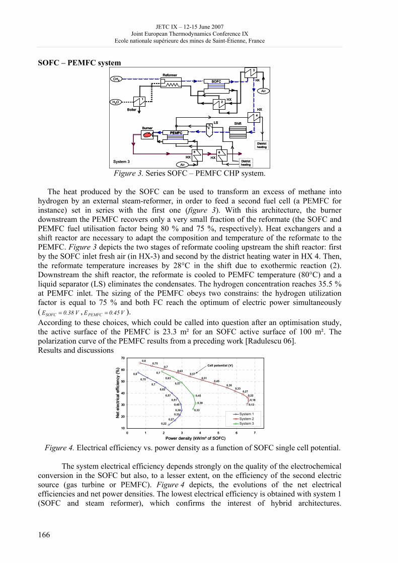
JETC IX – 12-15 June 2007 Joint European Thermodynamics Conference IX
Ecole nationale supérieure des mines de Saint-Étienne, France
166
SOFC – PEMFC system
System 3
Air
H2O
CH4
Reformer
SOFC
Burner
Boiler
HX
PEMFC
Shift
Air
HX
HX
Districtheating
HX
Districtheating
HX
21
3
4
5 6
LS
System 3
Air
H2O
CH4
Reformer
SOFC
Burner
Boiler
HX
PEMFCPEMFC
Shift
Air
HX
HX
Districtheating
HX
Districtheating
HX
21
3
4
5 6
LS
Figure 3. Series SOFC – PEMFC CHP system.
The heat produced by the SOFC can be used to transform an excess of methane into
hydrogen by an external steam-reformer, in order to feed a second fuel cell (a PEMFC for instance) set in series with the first one (figure 3). With this architecture, the burner downstream the PEMFC recovers only a very small fraction of the reformate (the SOFC and PEMFC fuel utilisation factor being 80 % and 75 %, respectively). Heat exchangers and a shift reactor are necessary to adapt the composition and temperature of the reformate to the PEMFC. Figure 3 depicts the two stages of reformate cooling upstream the shift reactor: first by the SOFC inlet fresh air (in HX-3) and second by the district heating water in HX 4. Then, the reformate temperature increases by 28°C in the shift due to exothermic reaction (2). Downstream the shift reactor, the reformate is cooled to PEMFC temperature (80°C) and a liquid separator (LS) eliminates the condensates. The hydrogen concentration reaches 35.5 % at PEMFC inlet. The sizing of the PEMFC obeys two constrains: the hydrogen utilization factor is equal to 75 % and both FC reach the optimum of electric power simultaneously ( V38.0ESOFC = , V45.0EPEMFC = ). According to these choices, which could be called into question after an optimisation study, the active surface of the PEMFC is 23.3 m² for an SOFC active surface of 100 m². The polarization curve of the PEMFC results from a preceding work [Radulescu 06]. Results and discussions
10
20
30
40
50
60
70
0 1 2 3 4 5 6 7
Power density (kW/m² of SOFC)
Net
ele
ctric
al e
ffici
ency
(%)
System 1System 2System 3
0,180,12
0,8
0,75
0,7
0,63
0,570,51
0,45
0,380,33
0,270,22
0,7
0,63
0,57
0,45
0,38
0,33
0,80,75
0,70,63
0,570,51
0,450,38
0,330,27
0,22
Cell potential (V)
10
20
30
40
50
60
70
0 1 2 3 4 5 6 7
Power density (kW/m² of SOFC)
Net
ele
ctric
al e
ffici
ency
(%)
System 1System 2System 3
0,180,12
0,8
0,75
0,7
0,63
0,570,51
0,45
0,380,33
0,270,22
0,7
0,63
0,57
0,45
0,38
0,33
0,80,75
0,70,63
0,570,51
0,450,38
0,330,27
0,22
Cell potential (V)
Figure 4. Electrical efficiency vs. power density as a function of SOFC single cell potential.
The system electrical efficiency depends strongly on the quality of the electrochemical
conversion in the SOFC but also, to a lesser extent, on the efficiency of the second electric source (gas turbine or PEMFC). Figure 4 depicts, the evolutions of the net electrical efficiencies and net power densities. The lowest electrical efficiency is obtained with system 1 (SOFC and steam reformer), which confirms the interest of hybrid architectures.
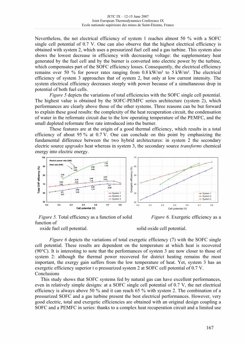
JETC IX – 12-15 June 2007 Joint European Thermodynamics Conference IX
Ecole nationale supérieure des mines de Saint-Étienne, France
167
Nevertheless, the net electrical efficiency of system 1 reaches almost 50 % with a SOFC single cell potential of 0.7 V. One can also observe that the highest electrical efficiency is obtained with system 2, which uses a pressurized fuel cell and a gas turbine. This system also shows the lowest decrease in efficiency with decreasing voltage: the supplementary heat generated by the fuel cell and by the burner is converted into electric power by the turbine, which compensates part of the SOFC efficiency losses. Consequently, the electrical efficiency remains over 50 % for power rates ranging from 0.8 kW/m² to 5 kW/m². The electrical efficiency of system 3 approaches that of system 2, but only at low current intensity. The system electrical efficiency decreases steeply with power because of a simultaneous drop in potential of both fuel cells.
Figure 5 depicts the variations of total efficiencies with the SOFC single cell potential. The highest value is obtained by the SOFC-PEMFC series architecture (system 2), which performances are clearly above those of the other systems. Three reasons can be but forward to explain these good results: the complexity of the heat recuperation circuit, the condensation of water in the reformate circuit due to the low operating temperature of the PEMFC, and the small depleted reformate flow rate introduced into the burner.
These features are at the origin of a good thermal efficiency, which results in a total efficiency of about 95 % at 0.7 V. One can conclude on this point by emphasizing the fundamental difference between the two hybrid architectures: in system 2 the secondary electric source upgrades heat whereas in system 3, the secondary source transforms chemical energy into electric energy.
50
60
70
80
90
100
0.2 0.3 0.4 0.5 0.6 0.7 0.8
Cell potential (V)
Tota
l CH
P ef
ficie
ncy
(%)
System 1System 2System 3
1,60,682,46
1,742,943,422,9
5,81
2,030,443,44
1,144,782,235,92
3,81
1,911,19
2,992,64
3,654,49
3,627,1
Electric power rate (kW)
Heat rate (kW)
50
60
70
80
90
100
0.2 0.3 0.4 0.5 0.6 0.7 0.8
Cell potential (V)
Tota
l CH
P ef
ficie
ncy
(%)
System 1System 2System 3
1,60,682,46
1,742,943,422,9
5,81
2,030,443,44
1,144,782,235,92
3,81
1,911,19
2,992,64
3,654,49
3,627,1
Electric power rate (kW)
Heat rate (kW)
20
30
40
50
60
70
0.2 0.3 0.4 0.5 0.6 0.7 0.8
Cell potential (V)
Exe
rget
ic e
ffici
ency
(%)
System 1System 2System 3
Figure 5. Total efficiency as a function of solid Figure 6. Exergetic efficiency as a
function of oxide fuel cell potential. solid oxide cell potential.
Figure 6 depicts the variations of total exergetic efficiency (7) with the SOFC single
cell potential. These results are dependent on the temperature at which heat is recovered (90°C). It is interesting to note that the performances of system 3 are now closer to those of system 2: although the thermal power recovered for district heating remains the most important, the exergy gain suffers from the low temperature of heat. Yet, system 3 has an exergetic efficiency superior t o pressurized system 2 at SOFC cell potential of 0.7 V. Conclusions
This study shows that SOFC systems fed by natural gas can have excellent performances, even in relatively simple designs: at a SOFC single cell potential of 0.7 V, the net electrical efficiency is always above 50 % and it can reach 65 % with system 2. The combination of a pressurized SOFC and a gas turbine present the best electrical performances. However, very good electric, total and exergetic efficiencies are obtained with an original design coupling a SOFC and a PEMFC in series: thanks to a complex heat recuperation circuit and a limited use
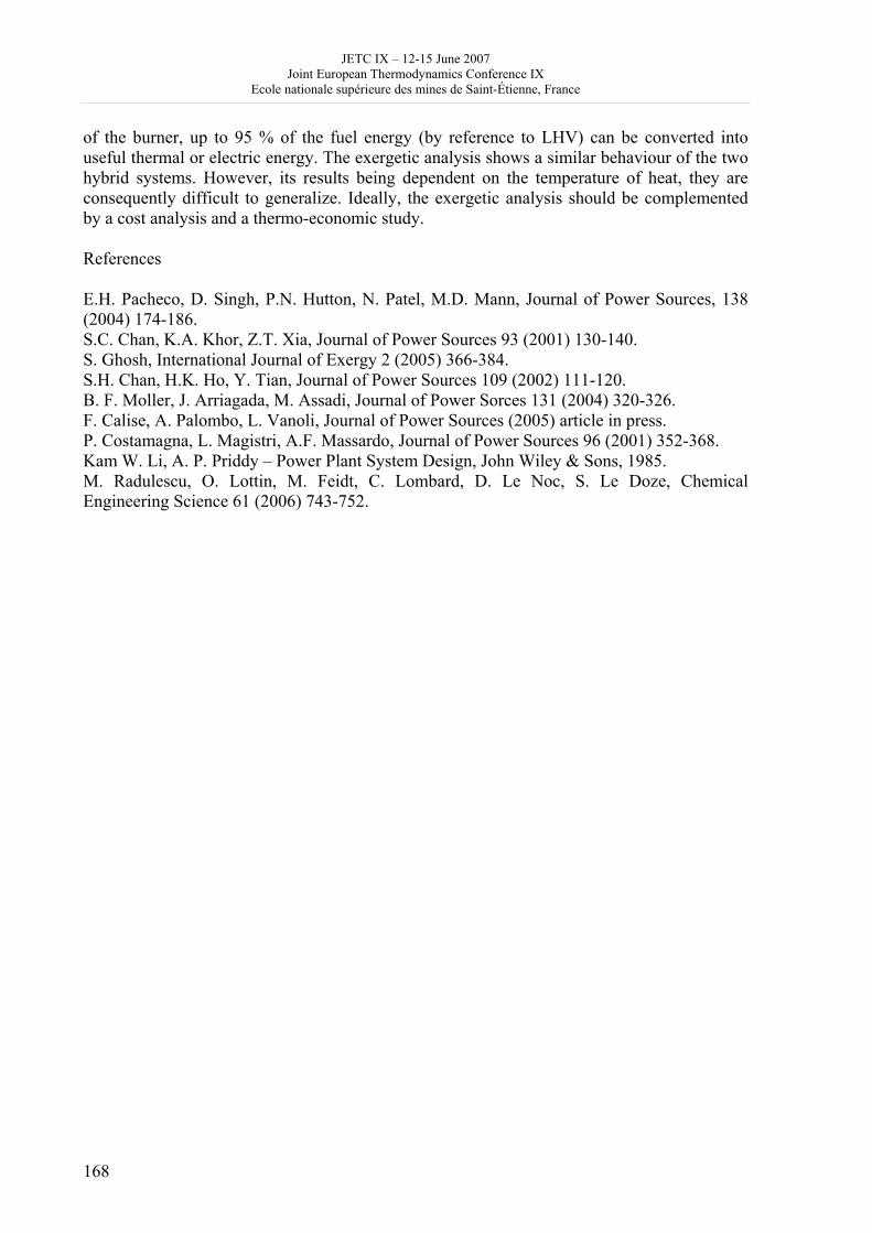
JETC IX – 12-15 June 2007 Joint European Thermodynamics Conference IX
Ecole nationale supérieure des mines de Saint-Étienne, France
168
of the burner, up to 95 % of the fuel energy (by reference to LHV) can be converted into useful thermal or electric energy. The exergetic analysis shows a similar behaviour of the two hybrid systems. However, its results being dependent on the temperature of heat, they are consequently difficult to generalize. Ideally, the exergetic analysis should be complemented by a cost analysis and a thermo-economic study.
References E.H. Pacheco, D. Singh, P.N. Hutton, N. Patel, M.D. Mann, Journal of Power Sources, 138 (2004) 174-186. S.C. Chan, K.A. Khor, Z.T. Xia, Journal of Power Sources 93 (2001) 130-140. S. Ghosh, International Journal of Exergy 2 (2005) 366-384. S.H. Chan, H.K. Ho, Y. Tian, Journal of Power Sources 109 (2002) 111-120. B. F. Moller, J. Arriagada, M. Assadi, Journal of Power Sorces 131 (2004) 320-326. F. Calise, A. Palombo, L. Vanoli, Journal of Power Sources (2005) article in press. P. Costamagna, L. Magistri, A.F. Massardo, Journal of Power Sources 96 (2001) 352-368. Kam W. Li, A. P. Priddy – Power Plant System Design, John Wiley & Sons, 1985. M. Radulescu, O. Lottin, M. Feidt, C. Lombard, D. Le Noc, S. Le Doze, Chemical Engineering Science 61 (2006) 743-752.
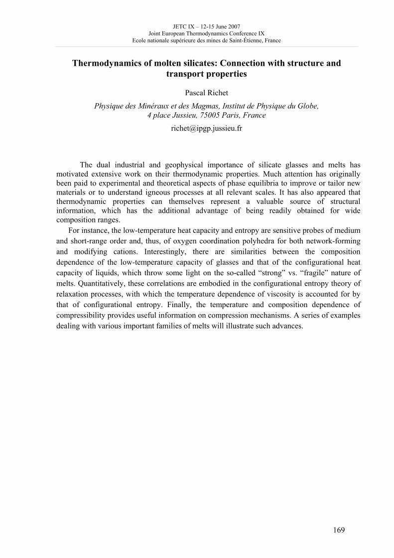
JETC IX – 12-15 June 2007 Joint European Thermodynamics Conference IX
Ecole nationale supérieure des mines de Saint-Étienne, France
169
Thermodynamics of molten silicates: Connection with structure and transport properties
Pascal Richet
Physique des Minéraux et des Magmas, Institut de Physique du Globe, 4 place Jussieu, 75005 Paris, France
[email protected] The dual industrial and geophysical importance of silicate glasses and melts has motivated extensive work on their thermodynamic properties. Much attention has originally been paid to experimental and theoretical aspects of phase equilibria to improve or tailor new materials or to understand igneous processes at all relevant scales. It has also appeared that thermodynamic properties can themselves represent a valuable source of structural information, which has the additional advantage of being readily obtained for wide composition ranges. For instance, the low-temperature heat capacity and entropy are sensitive probes of medium and short-range order and, thus, of oxygen coordination polyhedra for both network-forming and modifying cations. Interestingly, there are similarities between the composition dependence of the low-temperature capacity of glasses and that of the configurational heat capacity of liquids, which throw some light on the so-called “strong” vs. “fragile” nature of melts. Quantitatively, these correlations are embodied in the configurational entropy theory of relaxation processes, with which the temperature dependence of viscosity is accounted for by that of configurational entropy. Finally, the temperature and composition dependence of compressibility provides useful information on compression mechanisms. A series of examples dealing with various important families of melts will illustrate such advances.
JETC IX – 12-15 June 2007 Joint European Thermodynamics Conference IX
Ecole nationale supérieure des mines de Saint-Étienne, France
170
On thermal diffusion and convection in multicomponent mixtures with application to thermogravitational column
Ilya I. Ryzhkov1,2 and Valentina M. Shevtsova1
1MRC, Department of Chemical Physics, Universite Libre de Bruxelles CP 165/62, av. F.D. Roosevelt 50, B–1050 Brussels, Belgium
2Institute of Computational Modelling SB RAS, 660036 Krasnoyarsk, Russia
The theoretical framework for describing multicomponent mixtures with Soret effect is revised and extended. The separation ratio, a fundamental parameter characterizing the influence of thermal diffusion on convective phenomena, is generalized to multicomponent case. It is shown how to define this parameter for a particular component of the mixture. To characterize multicomponent system as a whole, the net separation ratio Ψ, which does not depend on the choice of solvent, is introduced. Based on these results, the dimensionless equations for convection in a multicomponent mixture are derived. The proposed formalism describes the system in such a way that the parameters and equations are similar to those used in binary case. It proves to be very helpful and efficient for studying convective flows and their stability in multicomponent mixtures with Soret effect.
The described formalism is applied to analyzing the steady state separation in thermogravitational column (TGC), which is a well-known technique for separating mixtures and measuring thermal diffusion coefficients. The approximation neglecting vertical diffusion in the column is employed and conditions for its validity are analyzed. The distributions of velocity, temperature, and composition in a multicomponent system are found. The relevant parameters here are the solutal Rayleigh numbers, which characterize the vertical separation of species, and the net solutal Rayleigh number R, which quantifies the overall effect of this separation on the system behaviour. It is shown that the key relation of TGC theory, which relates the vertical compositional gradients to the thermal diffusion coefficients, reduces to the dependence of the net separation ratio Ψ on the net solutal Rayleigh number R. A detailed study of this dependence is performed. The description of TGC in terms of these dimensionless parameters allows one to treat the relevant physical phenomena on a unified basis and reveals new peculiarities in the system behaviour. The evolution of vertical velocity and density profiles with changing the net separation ratio is investigated. It is shown that the stationary solution is unique for Ψ > –1, non-unique for –5 < Ψ < –1, and does not exist for Ψ < –5. A particular ternary mixture is considered and its behaviour in the column is analyzed. References I. Ryzhkov and V. Shevtsova. On thermal diffusion and convection in multicomponent mixtures with application to thermogravitational column. Physics of Fluids, 2007, accepted, in press.
JETC IX – 12-15 June 2007 Joint European Thermodynamics Conference IX
Ecole nationale supérieure des mines de Saint-Étienne, France
171
Aqueous solubility and partition coefficients of halogenated hydrocarbons as a function of molecular structure
Sabine Sarraute, Vladimir Majer, Margarida F. Costa Gomes
Laboratoire de Thermodynamique des Solutions et des Polymères, Université Blaise Pascal Clermont-Ferrand/CNRS, 63177 Aubière, France
[email protected] Abstract The aqueous solubilities of several halogenated hydrocarbons were studied between 274 and 313 K. The present experimental results exhibit an imprecision of ±5% and an estimated inaccuracy of ±10%. A combination with the data on pure solutes selected from the literature made it possible to calculate Henry’s law constants and the air-water partition coefficients. These different data were combinated with information from the literature and analysed with respect to the molecular structure of halogenated hydrocarbons. A simple group contribution concept was found to be useful for predicting the evolution of Henry’s law constants of alkanes, cycloalkanes and halogenated alkanes. Introduction The prediction of the transport and fate of hydrophobic organic chemicals in the environment requires a precise knowledge of their physical and chemical properties. One of the most important thermodynamic properties is the solubility in water because, together with the vapour pressure, it is essential for the calculation of several partion coefficients such as the air-water partition coefficient or the octanol-water coefficient [1,2]. Experimental All the solutes used were obtained from commercial sources with stated purities of at least 98 mol%. Distilled water was used as solvent. The experimental technique used in this work is based on a dynamic method and was previously described for measurements at high temperature [3]. The apparatus employed and the experimental procedure followed were described in detail in two previous publications [4,5]. The apparatus used is schematically represented in Figure 1. The saturated column (SC) was fill up with an inert stationary phase (Gaz Chrom R 60/80 for Alltech) impregnated with the organic solute and placed in the thermostatic bath (T). The liquid thermostat is contolled by a proportional-integral-derivative temperature controller from Tronac Inc., model PTC-40 which maintains the stability to within ±0.05 K in the whole temperature range of measurements. The water is pumped with a Gilson pump model 306 (P) operating in a constant-flow mode through the pre-heating coil into the saturation cell. The first step of the experimental procedure consists on the conditionning of the saturation column (Figure 1A). More than 10 mL of water are normally necessary to reach steady state. The extraction column (EC), previously conditionned with water, is then connected to the end of the system (Figure 1B). The solvent is pumped at flow rates between 0.1 and 0.3 mL/min, through a pre-heating coil, into the saturation cell containing the solute immobilized in a dry and clean solid stationary phase. The saturated solution is then pumped into an inverse phase analytical column where the solute is quantitatively retained. The organic compound is subsequently removed by back flushing this extaction column with an appropriate solvent, methanol in this
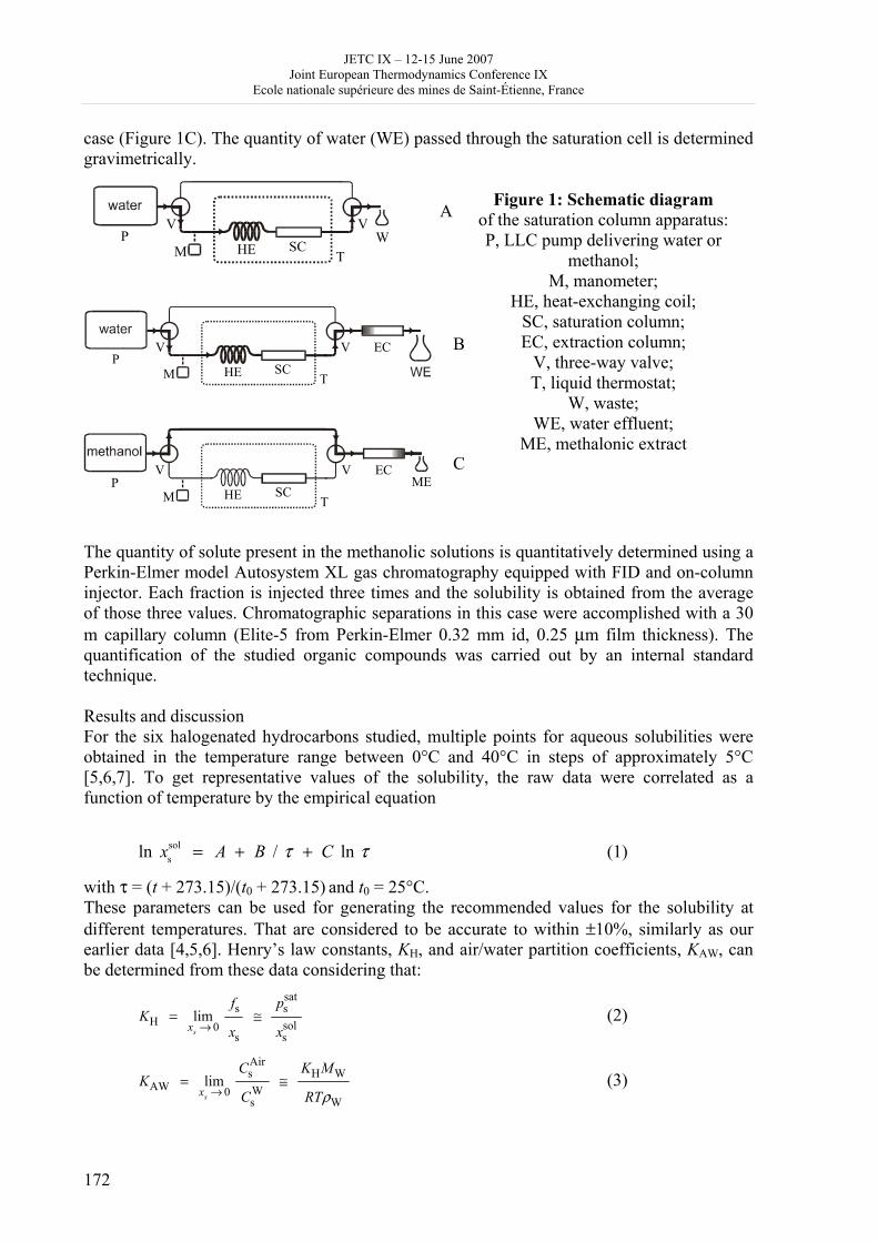
JETC IX – 12-15 June 2007 Joint European Thermodynamics Conference IX
Ecole nationale supérieure des mines de Saint-Étienne, France
172
case (Figure 1C). The quantity of water (WE) passed through the saturation cell is determined gravimetrically.
Figure 1: Schematic diagram
of the saturation column apparatus: P, LLC pump delivering water or
methanol; M, manometer;
HE, heat-exchanging coil; SC, saturation column; EC, extraction column;
V, three-way valve; T, liquid thermostat;
W, waste; WE, water effluent;
ME, methalonic extract
The quantity of solute present in the methanolic solutions is quantitatively determined using a Perkin-Elmer model Autosystem XL gas chromatography equipped with FID and on-column injector. Each fraction is injected three times and the solubility is obtained from the average of those three values. Chromatographic separations in this case were accomplished with a 30 m capillary column (Elite-5 from Perkin-Elmer 0.32 mm id, 0.25 μm film thickness). The quantification of the studied organic compounds was carried out by an internal standard technique. Results and discussion For the six halogenated hydrocarbons studied, multiple points for aqueous solubilities were obtained in the temperature range between 0°C and 40°C in steps of approximately 5°C [5,6,7]. To get representative values of the solubility, the raw data were correlated as a function of temperature by the empirical equation
ττ ln/ln sols CBAx ++= (1)
with τ = (t + 273.15)/(t0 + 273.15) and t0 = 25°C. These parameters can be used for generating the recommended values for the solubility at different temperatures. That are considered to be accurate to within ±10%, similarly as our earlier data [4,5,6]. Henry’s law constants, KH, and air/water partition coefficients, KAW, can be determined from these data considering that:
sols
sats
s
s0H lim
x
p
x
fK
sx≅=
→ (2)
W
WHWs
Airs
0AW limρRT
MK
C
CK
sx≅=
→ (3)
A
B
C
M P
HE SC
EC
T
V V
M P
HE SC
EC ME
T
V V
M P
HE SC W
T
V V
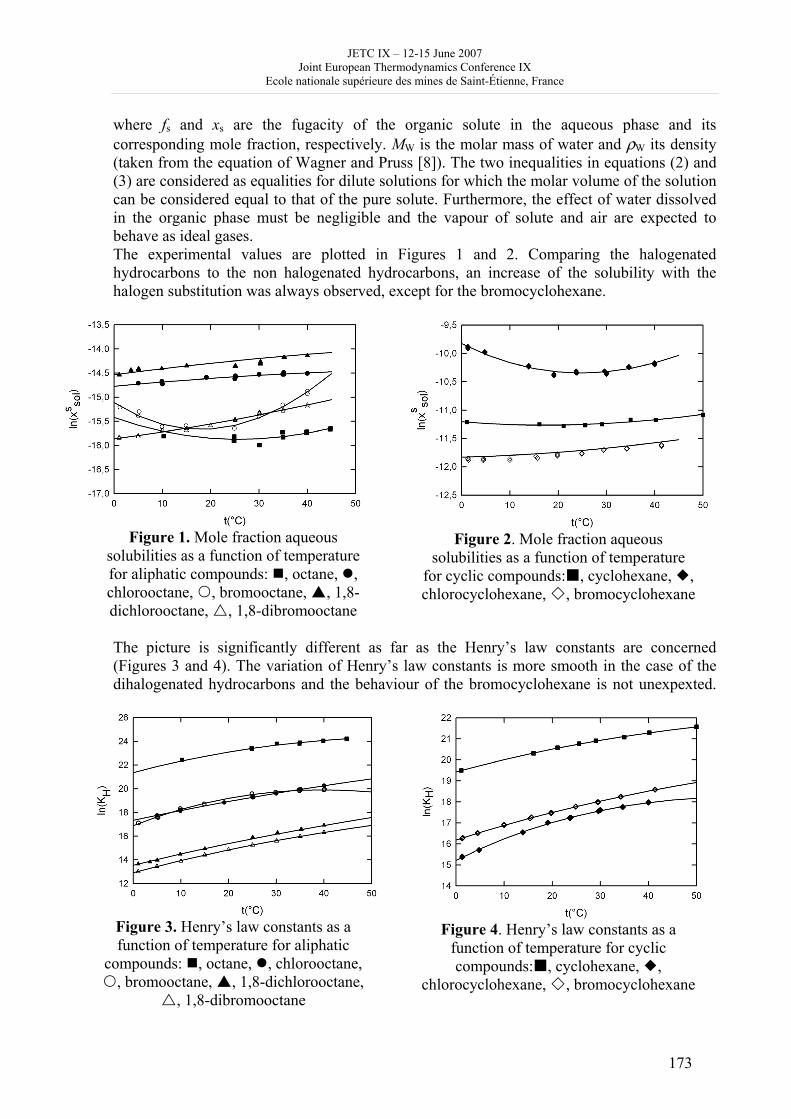
JETC IX – 12-15 June 2007 Joint European Thermodynamics Conference IX
Ecole nationale supérieure des mines de Saint-Étienne, France
173
where fs and xs are the fugacity of the organic solute in the aqueous phase and its corresponding mole fraction, respectively. MW is the molar mass of water and ρW its density (taken from the equation of Wagner and Pruss [8]). The two inequalities in equations (2) and (3) are considered as equalities for dilute solutions for which the molar volume of the solution can be considered equal to that of the pure solute. Furthermore, the effect of water dissolved in the organic phase must be negligible and the vapour of solute and air are expected to behave as ideal gases. The experimental values are plotted in Figures 1 and 2. Comparing the halogenated hydrocarbons to the non halogenated hydrocarbons, an increase of the solubility with the halogen substitution was always observed, except for the bromocyclohexane.
Figure 1. Mole fraction aqueous
solubilities as a function of temperature for aliphatic compounds: , octane, , chlorooctane, , bromooctane, , 1,8-dichlorooctane, , 1,8-dibromooctane
Figure 2. Mole fraction aqueous
solubilities as a function of temperature for cyclic compounds: , cyclohexane, , chlorocyclohexane, , bromocyclohexane
The picture is significantly different as far as the Henry’s law constants are concerned (Figures 3 and 4). The variation of Henry’s law constants is more smooth in the case of the dihalogenated hydrocarbons and the behaviour of the bromocyclohexane is not unexpexted.
Figure 3. Henry’s law constants as a function of temperature for aliphatic
compounds: , octane, , chlorooctane, , bromooctane, , 1,8-dichlorooctane,
, 1,8-dibromooctane
Figure 4. Henry’s law constants as a function of temperature for cyclic compounds: , cyclohexane, ,
chlorocyclohexane, , bromocyclohexane
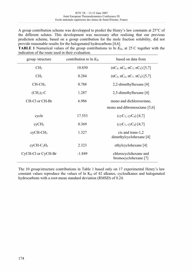
JETC IX – 12-15 June 2007 Joint European Thermodynamics Conference IX
Ecole nationale supérieure des mines de Saint-Étienne, France
174
A group contribution scheme was developped to predict the Henry’s law constants at 25°C of the different solutes. This development was necessary after realising that our previous prediction scheme, based on a group contribution for the mole fraction solubility, did not provide reasonable results for the halogenated hydrocarbons [4,6]. TABLE 1 Numerical values of the group contributions to ln KH, at 25 C together with the indication of the route used in their evaluation.
group /structure contribution to ln KH based on data from
CH3 10.850 (nC5, nC6, nC7, nC8) [5,7]
CH2 0.284 (nC5, nC6, nC7, nC8) [5,7]
CH-CH3 0.788 2,2-dimethylhexane [4]
(CH3)2-C 1.287 2,5-dimethylhexane [4]
CH-Cl or CH-Br 6.986 mono and dichlorooctane,
mono and dibromooctane [5,6]
cycle 17.553 (cyC7, cyC8) [4,7]
cyCH2 0.369 (cyC7, cyC8) [4,7]
cyCH-CH3 1.327 cis and trans-1,2 dimethylcyclohexane [4]
cyCH-C2H5 2.323 ethylcyclohexane [4]
CyCH-Cl or CyCH-Br -1.849 chlorocyclohexane and bromocyclohexane [7]
The 10 group/structure contributions in Table 1 based only on 17 experimental Henry’s law constant values reproduce the values of ln KH of 42 alkanes, cycloalkanes and halogenated hydrocarbons with a root-mean standard deviation (RMSD) of 0.24.
JETC IX – 12-15 June 2007 Joint European Thermodynamics Conference IX
Ecole nationale supérieure des mines de Saint-Étienne, France
175
References
[1] Boethling R. S., Mackay D. “Handbook of property estimation methods for chemicals-environmental and health sciences”, Lewis Publishers, 2000. [2] Mackay D. “Multimedia environmental models-The fugacity approach”, Lewis Publishers Inc., 1991. [3] Miller D.J., Hawthorne S.B., 1998. Method for determining the solubilities of hydrophobic organics in sbubcritical water. Anal. Chem. 70,1618-1621. [4] Dohányosová P., Sarraute S., Dohnal V., Majer V., Costa Gomes M., 2004. Aqueous solubility and related thermodynamic functions of nonaromatic hydrocarbons as a function of molecular structure. Ind. Eng. Chem. Res. 43, 2805-2815. [5] Sarraute S., Delepine, H., Costa Gomes M.F., Majer V., 2004. Aqueous solubility, Henry’s law constants and air/water partition coefficients of n-octane and two halogenated octanes. Chemosphere 57, 1543-1551. [6] Sarraute S., Mokbel I., Costa Gomes M.F., Majer V., Delepine, H., Jose J., 2006. Vapour pressures, aqueous solubility, Henry’s law constants and air/water partition coefficients of 1,8-dichlorooctane and 1,8-dibromooctane. Chemosphere 2006, 64, 1829-1836. [7] Sarraute S., Mokbel I., Costa Gomes M.F., Majer V., Jose J., 2006. Vapour pressures, aqueous solubility, Henry’s law constants and air/water partition coefficients of chloroccyclohexane and bromocyclohexane. Atmos. Environ. (in preparation) [8] Wagner W., Pruss A., 1993. Internationnal equations for saturation properties of ordinary water substance. Revised according to the international temperature scale of 1990. J. Phys. Chem. Ref. Data 22, 783-787.
JETC IX – 12-15 June 2007 Joint European Thermodynamics Conference IX
Ecole nationale supérieure des mines de Saint-Étienne, France
176
Monomolecular fraction in real gases
Boris Sedunov
Russian New University, Moscow
[email protected] Introduction The aim of this report is to show a new thermodynamic approach to real gases, joining in one picture the density D, pressure P, internal energy E, Gibbs G and Helmholz F free energies, entropy S and heat capacity Cv. This approach is based on a very important variable – the monomolecular fraction density (MFD). The approach is phenomenological and one of its goals is to develop the methods of computational analysis of experimental data about thermophysical properties of real gases capable to throw more light on mechanisms of intermolecular interactions in real gases.
The contemporary level of knowledge of the interatomic or intermolecular interaction potential does not provide an effective utilization of microscopic approaches, such as the density matrix or molecular dynamics methods, for precise calculation of the real gases thermophysical properties. The theoretical assumptions about the type and parameters of the van der Waals forces are rather approximate and do not match the precision of the experimental data. To move forward in this direction it is necessary both to constantly improve the precision of experimental data about thermophysical properties of real gases and to improve the methods of the interaction potential parameters computation based on these data. The suggested here phenomenological and thermodynamics based approach avoids any assumptions about interatomic and intermolecular interactions, but nevertheless leads to fundamental results that help to interpret and practically use experimental data.
Possible practical applications of this research may be in the next fields:
- more effective utilization of databases on thermophysical properties of real gases in the computer aided design and control of chemical and material technologies;
- an improved precision of the databases through the crosscorrelation of different thermodynamic functions and MFD;
- stimulation and targeting of new experimental research works in order to precise the details of the interatomic interaction mechanisms and van der Waals forces.
Physical and virtual cluster fractions in a real gas A real gas is usually considered as a mixture of fractions with different numbers N of molecules in clusters [1]: single molecules (monomers), dimers, trimers, and larger clusters. The monomolecular (monomer) fraction can be defined as the part of a real gas, which molecules are temporarily far enough from other molecules, and their interactions with the rest of gas may be considered as negligible. The monomer fraction is an ideal gas dissolved in the rest of a real gas. Its introduction is the next step after the ideal gas model. The MFD, Dm , is the number of moles of the monomer fraction in a unit of volume. Its values may be derived from the D (P,T) experimental data without any limitations on the pressure value.
JETC IX – 12-15 June 2007 Joint European Thermodynamics Conference IX
Ecole nationale supérieure des mines de Saint-Étienne, France
177
Quite similarly, the dimer fraction can be defined as the part of a real gas consisting of pairs of molecules, temporarily joined together in a relatively stable formation or repulsing from each other, with a negligibly small interaction with the rest of gas. The dimer fraction behaves also as an ideal gas with a complex internal movement depending on a type of the intermolecular interaction potential. The same is valid for larger cluster fractions. According to the theory of chemical equilibrium, in a real gas the partial concentration DN of every cluster should be proportional to the N–th power of the monomolecular molar density Dm , with an equilibrium cluster formation constant CN (T).
It is important to note that between molecules not only attraction forces, producing real physical clusters with an equilibrium constant CPN (T), but also repulsion forces act. They produce an appearance of some virtual cluster with negative equilibrium constant - CVN (T). Index P is used to mark real physical clusters and V - virtual negative clusters. So, an interaction of monomers results in appearance of the excluded volume CV2 (T) and attraction volume CP2 (T), forming the well known second virial coefficient C2 (T) = CP2 (T) - CV2 (T). For a larger cluster its equilibrium constant CN (T) also may be presented as a sum of the physical CP (T) and virtual parts - CVN (T): CN (T) = CPN (T) - CVN (T). There is an active discussion in literature about the precise definition of the physical cluster [2]. But in our phenomenology the N-th order cluster have pure mathematical sense, joining together its physical and virtual features in the N-th order terms of series expansions D (Dm ) and P (Dm ).
Historically clusters in real gases have been introduced to build the methods and interpret the results of virial expansions of P (D). Many theoretical works have been based on the so called Feynman’s diagrams [3], reflecting different isomers of clusters with the same order. Nevertheless, the virial approach to real gases, being based on the total density D instead of the monomer density Dm , does not match in a full scale with the chemical equilibrium theory. It might be explained by difficulties of the partial densities determination basing on the experimental values of the total density. To build the bridge between virial and chemical approaches it is essential to find the way of deriving from the available thermophysical data the molar density of the monomer fraction, MFD, and to base the theory of real gases on this value, as a fundamental variable.
Generalized Sackur-Tetrode equation for the entropy of a real gas We build the MFD determination on the equation for the entropy Si of a monatomic ideal gas that has been suggested by Otto Sackur and Hugo Tetrode in 1912 basing on the old quantum theory [4]. This equation in a compact form [5] may be expressed as:
Si = R (2.5 + ln (Vi /Vq )), (1)
where Vi is the molar volume of the ideal gas, Vq = h3NA4 /(2πmRT)3/2 - the molar quantum volume
that is proportional to the third degree of the thermal de Broglie wavelength, h – Plank’s constant, m – molecular weight in kg/mol, NA – Avogadro number, R – universal gas constant. The Sackur-Tetrode equation was a remarkable breakthrough from the classical thermodynamics to the emerging quantum picture of Nature and stimulated multiple theoretical and experimental investigations. It was experimentally confirmed for noble gases, starting from the Third Thermodynamics Law at zero T.
From the equation (1) an expression for Gibbs free energy, Gi , of the monatomic ideal gas results:
Gi = RT ln (D Vq ). (2)
In an equilibrium state of a real gas the Gibbs free energy GN for any fraction, including the Gibbs free energy Gm for monomer fraction, should be the same and should coincide with the
JETC IX – 12-15 June 2007 Joint European Thermodynamics Conference IX
Ecole nationale supérieure des mines de Saint-Étienne, France
178
Gibbs free energy G for total real gas: GN = Gm = G. It is a key point to calculate the Dm values basing on the experimental data D (P). It is useful to divide the Gibbs free energy on its translational, Gtr , and internal movements, Gint , parts. The second part can be found for any temperature as a limit of G at pressure coming to zero. For monatomic gases Gint = 0 and Gtr = G . The translational part of G can be found as: Gtr = G - Gint . The translational part of Gm , Gmtr = 2.5RT – T Smtr , for the monomer fraction, as an ideal gas, can be written as:
Gmtr = RT ln (Dm Vq ). (3)
Therefore, the translational part of G for total gas corresponds to the equation:
Gtr = H - Eint – T (S - Sint ) = RT ln (Dm Vq ). (4)
Here H is the molar enthalpy, Eint and Sint – the molar energy and entropy of the clusters’ internal movements in the real gas.
From this equation follows the generalized Sackur-Tetrode equation for the real gas entropy: S = (H - Eint ) / T + Sint - RT ln (DmVq ). (5)
The author came to this equation after attempts to find the approximation for S (P,T ) [6]. But in a final version it is free from any approximations and assumptions about the intermolecular interaction mechanisms. All pressure dependent details of these mechanisms are hidden in the enthalpy of a real gas. It may sound surprising, but this equation has been proven to be valid also for condensed matter that confirms the correctness of the Dm computation in all available range of pressures.
Utilization of the MFD as an argument for the density and pressure series expansions
Having in mind that Gint is independent on pressure, it is possible to apply the thermodynamic equation VPG
T=∂∂ / only to Gtr , given by (4), and to write a differential equation for the MFD:
DRTDPD mTm =∂∂ . (6)
The numerical integration of this equation returns the Dmj (Pj ,T ) values for any temperature and pressure. This integration is a very delicate procedure and requires a high precision of the initial data Dj (Pj , T ) with a small enough value of the pressure step Pj+1 - Pj .
After receiving the Dmj (Pj ,T ) values for a fixed T the total pressure P can be expressed as a series expansion that may be interpreted as a sum of partial pressures of fractions:
P = RT Dm (1 + ∑∞
=2NNC Dm
(N - 1)) . (7)
As it was already noted, this equation contains both physical and virtual parts of the CN . The total density D can be expressed in a similar way:
D = Dm (1 + ∑∞
=2NNC N Dm
(N – 1) ) . (8)
Experimental data processing and some preliminary results So, for D (Dm ) and P (Dm ) a system of coherent equations (7, 8) is valid. This coherence and crosscorrelation helps in finding the equilibrium constants CN (T). It serves both as a tool and a criterion of the joint series expansion of experimental data for P (Dm ), D (Dm ), preventing from falling into the well known problem of polynomial oscillation at series expansions. It
JETC IX – 12-15 June 2007 Joint European Thermodynamics Conference IX
Ecole nationale supérieure des mines de Saint-Étienne, France
179
helps also to throw away the numbers N not presented in the joint series expansion. It is very important to prevent from the series expansion program catching for the nonexistent numbers.
As a source of experimental data the online database of the NIST (the USA National Institute of Standards and Technology) [7] for atomic and molecular gases is used. This database contains comprehensive data for 75 substances given with 5 decimal digits. At the first step the range of Pj (T), where only the terms of the second and the third order are essential, is selected to find C2 and C3. Then, the working range of Pj (T) is step-by-step expanded to find C4 and C5 and to proceed further. The found values of CN (T) are used to compare the polynomial approximations for pressure and density with their real values. The computation process may be stopped and regarded as correct, if the deviation of the approximation is of the same order of magnitude, as the occasional spread of the initial Dj (Pj , T ) data. It is possible also to step from the investigated range of P in a supersaturated state of a real gas just to estimate the clusters populations change. It may be used in the branch of the nucleation processes research, based on the virial coefficients values [7].
Approximations for Gibbs G and Helmholz F free energies, based on the found values for Dm and CN, possess smaller spreads than the database values resulting from calorimetric measurements. It opens the way to correct the existing databases. And also the MFD tables can be added to existing databases to expand their cognitive power and practical value.
For the moment, the next real gases have been investigated: Helium, Parahydrogen, Argon, Nitrogen, Methane, Water vapor. For all investigated gases a discrete structure of the series expansion is discovered. That means an absence of some numbers N in the power expansions. So, for Argon, Parahydrogen, Methane and Nitrogen it was impossible to notice any traces of the C4 (T), but in Water this coefficient has a noticeable value that reflects quite different type (polar instead of the van der Waals) of the intermolecular interaction. It should be noted that the discrete structure of the MFD based series expansions disappears in ordinary virial expansions. That means the virial expansions are less informative than the MFD based.
The MFD based series expansions of the internal energy E and heat capacity Cv give temperature dependences for the van der Waals bond energies for small order clusters and for the excluded volume that provide possibilities to understand better the form of the intermolecular potential and the nature of the van der Waals forces.
Conclusion The introduction of Dm expands power of the computer assisted analysis of a wide series of thermodynamic functions of real gases to throw more light on the interactions of atoms and molecules. The found facts inspire and provide directions for more profound experimental and theoretical studies of real gases and condensed matter.
JETC IX – 12-15 June 2007 Joint European Thermodynamics Conference IX
Ecole nationale supérieure des mines de Saint-Étienne, France
180
References:
[1] Ford I.J. Statistical mechanics of nucleation: a review. Proc. Instn Mech. Engrs. Part C: J. Mechanical Engineering Science, 2004, 218 (C), 883 [2] Schaaf P., Senger B., and Reiss H. Defining Physical Clusters in Nucleation Theory from the N-Particle Distribution Function. J. Phys. Chem. B, 1997, 101 (43), 8740; Kusaka I. and Oxtoby D.W. Identifying Physical Clusters in Vapor Phase Nucleation. J. Chem. Phys. 1999, 110 (20), 5249; Harris S.S. and Ford I.J. A Dynamical Definition of Quasibound Molecular Clusters. J. Chem. Phys. 2003, 118 (20), 9216 [3] Feynman R. Statistical mechanics; A set of lectures; 1972, (W.A. Benjamin, Inc.) Massachusetts [4] Sackur O. 1913, Ann. der Physik 40, 67; Tetrode H. 1912, Ann. der Physik 38, 434 [5] Kittel Ch. Thermal physics; 1970, (John Wiley and Sons, Inc.) New York [6] Sedunov B. An analysis of interatomic interactions in simple condensed matter; 2001, E-Journal “Investigated in Russia” http://zhurnal.ape.relarn.ru/articles/2001/079e.pdf [7] NIST - Thermophysical Properties of Fluid Systems, http://webbook.nist.gov/chemistry/fluid/ [8] Ford I.J. Virial/Fisher Models of Molecular Cluster Populations. J. Chem. Phys. 1997, 106 (23), 9734
JETC IX – 12-15 June 2007 Joint European Thermodynamics Conference IX
Ecole nationale supérieure des mines de Saint-Étienne, France
181
Evolutions thermodynamics of a driving fluid in a cylinder with valves
M.Serier, A.Serier
Laboratory of covers, materials and environment M' Hamed Bougara university, 35000 Boumerdes - Algeria
[email protected] Introduction To allow the estimation of the energy level of the fluid and its variation in time, it is necessary to know in every point of the gas mixture and all the time, its pressure, its temperature, its density and its chemical composition. Whatever are the undergone transformations, present gases in the cylinder are supposed in balance thermodynamics. I – Modelling The transformations thermodynamics governing the evolution of the fluid are represented on her figure1
1. Compression – relaxation The works of compression and relaxation are obtained by the energy balance
ccc QUw −Δ= (a) ; ddd QUw −Δ= (b) (1) UΔ : is the variation of the internal energy of the fluid, obtained by the following relations:
( )[ ]dTcmcmmUT
Tvfuvmcarac ∫ ++=Δ
2
1
0 (a) ; ( ) dTcmmmU vfu
T
Tcarad ∫ ++=Δ
4
3
0 (b) (2)
T is the temperature of the fluid, ma mass of the air, the mcar the mass of the fuel and m0 the mass of the residual fluid; The thermal capacity molar expresses himself by:
2TTC iivi δβα ++= ; Kmol
cal.
77.4=α (3)
The coefficients iβ and iδ are given according to the nature of the gas. The expressions of the thermal capacities massiques in constant volume of smokes ( cvfu ) and mixture ( cvm ) are given by:
2210 TaTaacvfu ++= (a) ; 2
210 TbTbbcvm ++= (b) (4) The coefficients a0, a1, a2, b0, b1 and b2 depend on the number of atoms of carbon and on
hydrogen contained in the unity of mass of the fuel, the excess of air, coefficients β , δ , of the thermal capacities molars, and the real power comburivore of the fuel
( ) aa MeyxV +⎟⎠⎞
⎜⎝⎛ += 1
477.4 , Where Ma is the mass molar of the air (5)
The quantities of heat Qc and Qd exchanged between the fluid and the internal wall of the cylinder during the compression and during the relaxation are determined by expression:
( ) tTTSQ mcpmcc ′Δ−= α (a) ; ( ) tTTSQ mdpmdd ′Δ−= α (b) ( )⎥⎦⎤
⎢⎣⎡ +−Δ=′Δ
πθτ1tt (6)
tΔ corresponds to the quarter of the time of cycle of the transformations , or N30 with N
rotation speed; τ is the angular delay with the closing of the inlet valve during
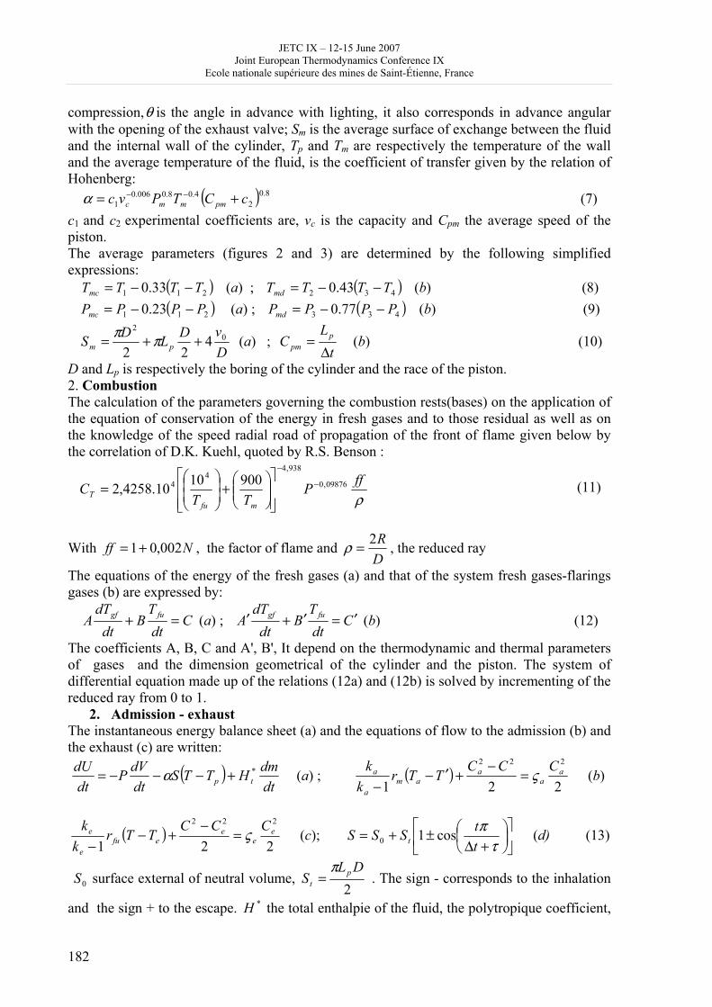
JETC IX – 12-15 June 2007 Joint European Thermodynamics Conference IX
Ecole nationale supérieure des mines de Saint-Étienne, France
182
compression,θ is the angle in advance with lighting, it also corresponds in advance angular with the opening of the exhaust valve; Sm is the average surface of exchange between the fluid and the internal wall of the cylinder, Tp and Tm are respectively the temperature of the wall and the average temperature of the fluid, is the coefficient of transfer given by the relation of Hohenberg:
( ) 8.02
4.08.0006.01 cCTPvc pmmmc += −−α (7)
c1 and c2 experimental coefficients are, vc is the capacity and Cpm the average speed of the piston. The average parameters (figures 2 and 3) are determined by the following simplified expressions:
( )211 33.0 TTTTmc −−= (a) ; ( )432 43.0 TTTTmd −−= (b) (8) ( )211 23.0 PPPPmc −−= (a) ; ( )433 77.0 PPPPmd −−= (b) (9)
DvDLDS pm
02
422
++= ππ (a) ; t
LC p
pm Δ= (b) (10)
D and Lp is respectively the boring of the cylinder and the race of the piston. 2. Combustion The calculation of the parameters governing the combustion rests(bases) on the application of the equation of conservation of the energy in fresh gases and to those residual as well as on the knowledge of the speed radial road of propagation of the front of flame given below by the correlation of D.K. Kuehl, quoted by R.S. Benson :
ρffP
TTC
mfuT
09876,0
938,44
4 9001010.4258,2 −
−
⎥⎥⎦
⎤
⎢⎢⎣
⎡⎟⎟⎠
⎞⎜⎜⎝
⎛+⎟
⎟⎠
⎞⎜⎜⎝
⎛= (11)
With Nff 002,01+= , the factor of flame and DR2=ρ , the reduced ray
The equations of the energy of the fresh gases (a) and that of the system fresh gases-flarings gases (b) are expressed by:
CdtT
Bdt
dTA fugf =+ (a) ; C
dtT
Bdt
dTA fugf ′=′+′ (b) (12)
The coefficients A, B, C and A', B', It depend on the thermodynamic and thermal parameters of gases and the dimension geometrical of the cylinder and the piston. The system of differential equation made up of the relations (12a) and (12b) is solved by incrementing of the reduced ray from 0 to 1.
2. Admission - exhaust The instantaneous energy balance sheet (a) and the equations of flow to the admission (b) and the exhaust (c) are written:
( )dtdmHTTS
dtdVP
dtdU
tp*+−−−= α (a) ; ( )
221
222a
aa
ama
a CCCTTr
kk ς=
−+′−
− (b)
( )221
222e
ee
efue
e CCCTTr
kk ς=
−+−
− (c); ⎥
⎦
⎤⎢⎣
⎡⎟⎠⎞
⎜⎝⎛
+Δ±+=
τπ
ttSSS t cos10 (d) (13)
0S surface external of neutral volume, 2
DLS p
t
π= . The sign - corresponds to the inhalation
and the sign + to the escape. *H the total enthalpie of the fluid, the polytropique coefficient,
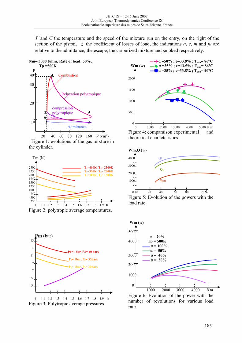
JETC IX – 12-15 June 2007 Joint European Thermodynamics Conference IX
Ecole nationale supérieure des mines de Saint-Étienne, France
183
T ′ and C the temperature and the speed of the mixture run on the entry, on the right of the section of the piston, ς the coefficient of losses of load, the indications a, e, m and fu are relative to the admittance, the escape, the carburized mixture and smoked respectively.
Nm= 3000 t/min, Rate of load: 50%, Tp =500K P 40 4 Combustion 30 Relaxation polytropique 20 compression 3 polytropique 5 6 Escape 10 1 2 Admittance 20 40 60 80 120 160 V (cm3) Figure 1: evolutions of the gas mixture in the cylinder. Tm (K) 2500 T1=400K, T3= 2500K 2250 T1=350K, T3= 2000K 2000 T1=300K, T3= 1500K 1750 1500 1250 1000 750 500 250 1 1.1 1.2 1.3 1.4 1.5 1.6 1.7 1.8 1.9 k
Figure 2: polytropic average temperatures.
Pm (bar) 15 13 P1= 1bar, P3= 40 bars 11 P1= 1bar, P3= 35bars 9 P1= 1bar, P3= 30bars 7 5 3 1 1.1 1.2 1.3 1.4 1.5 1.6 1.7 1.8 1.9 k
Figure 3: Polytropic average pressures.
α =50% ; e=33.8% ; Teau= 86°C Wm (w) α =35% ; e=13.5% ; Teau= 86°C α =35% ; e=33.8% ; Teau= 40°C 2000 1500 1000 500 0 0 1000 2000 3000 4000 5000 Nm Figure 4: comparaison experimental and theoretical characteristics Wm,Q (w) 4000 Qf 3000 Qp 2000 1000 Wm 0 10 20 40 60 80 α % Figure 5: Evolution of the powers with the load rate
Wm (w) 5000 e = 20% 4000 Tp = 500K α = 100% α = 50% 3000 α = 40% α = 30% 2000 1000 0 1000 2000 3000 4000 Nm Figure 6: Evolution of the power with the number of revolutions for various load rate.
JETC IX – 12-15 June 2007 Joint European Thermodynamics Conference IX
Ecole nationale supérieure des mines de Saint-Étienne, France
184
II - Confrontation theory - experience The results of this confrontation are represented on the figure 4 where we notice a rather good concordance between the theory and the experience as regards the output power. To obtain a global representation of the consequent performances of the transformations of the driving fluid, we presented on figures 5 the evolutions of the output power Wm, lost in the walls of the cylinder Qp and in the exhaust gases Qf according to the rate of load. The increasing pace of these evolutions for α =30 to 60 % seems to reach a landing for α = 60 to 100 %. The figure 6 brings to light for various regime and various rate of load the evolution of the output power developed by gases. III - Conclusion This study which uses at the same time analytical and empirical equations, is a tool of analysis and interpretation of the phenomena controlling the evolution of a driving fluid within a cylinder with valves. It allows, moreover, the relatively detailed analysis of the distribution of the energies developed by the transformations of the fluid. It presents, a good coherence with the experimental results obtained on a test bench of a single four –stroke spark-ignition gas engine cylinder. Bibliography [ ]1 Benson (R.S.), Annand (W.J.D.), Baruah (P.C.).- A simulation model including intake and exhaust system for a single four-stroke cycle spark-ignition engine. Int. J. Mech. Sci.,1975, v. 17, p. 97-124. [ ]2 Hohenberg (G.F.).- Advanced approches for heat transfer calculations. SAE/SP-79-449,1979, n° 790825, p. 61 – 79. [ ]3 Heywood (J. B.).- Internal Combustion Engines Fundamentals. McGraw-Hill Book Company, New York, 1988. [ ]4 Gunea (C.), Razavi (M. R.) et Karim (G. A.).- The effects of pilot fuel quality on dual-fuel engine ignition delay.SAE Paper, 1998, n° 982453. [ ]5 Roberge ( B).- Seuil minimal d'émission d'oxyde de carbone en rapport avec les émissions des oxydes d'azote dans les gaz d'échappement de véhicules au propane. Montréal, IRSST, Études et recherches R-218, 1999, 23 p.
JETC IX – 12-15 June 2007 Joint European Thermodynamics Conference IX
Ecole nationale supérieure des mines de Saint-Étienne, France
185
Constant-Hamiltonian paths for power-producing relaxation of non-linear resources
Stanislaw Sieniutycz
Faculty of Chemical and Process Engineering Warsaw University of Technology
PL 00-645, 1 Waryńskiego Street, Warsaw, Poland
Systems with active (i.e. power-producing) relaxation to the equilibrium are modeled and analyzed. The thermodynamic approach includes the simulation and modeling of nonlinear energy converters, in particular radiation engines. Thermodynamics leads to expressions for the converter’s efficiency and limiting generated work in terms of the entropy production. The exhaust of a resource leads to a dynamical problem characterized by a finite rate of the decay of the resource thermal potential. The real work is a cumulative effect obtained in a system containing: a resource, a sequence of engines, and an infinite bath. Nonlinear modeling involves methods of dynamic optimization such as maximum principles, variational calculus and dynamic programming. A main result of modeling is a finite-rate generalization of the classical, reversible work potential (exergy). The generalized function depends on thermal coordinates and a dissipation index, h, in fact the Hamiltonian of the optimization problem of minimum entropy production. This function implies stronger bounds on work delivered or supplied than the reversible work potential. As an example of the kinetic work limit in a nonlinear system, generalized exergy of radiation fluid is estimated in terms of finite rates, quantified by Hamiltonian h. Applying an involved mathematical analysis that eliminates the time variable by a Lagrange multiplier, this research formulates and discusses important quantitative and qualitative aspects of constant-Hamiltonian paths for power-producing relaxation. Keywords: thermal efficiency, thermal machines, entropy production, nonlinear engines
JETC IX – 12-15 June 2007 Joint European Thermodynamics Conference IX
Ecole nationale supérieure des mines de Saint-Étienne, France
186
Thermodynamically Guided Modelling and Intensification of Steady State Processes.
M.Sorina , F. Rheaulta and B. Spinnerb a CANMET Energy Technology Centre -Varennes, 1615 Lionel-Boulet, P.O. Box 4800,
Varennes, Quebec, J3X 1S6, Canada, Tel: (450) 652-3513, Fax: (450) 652-0999, b CNRS-IMP, Institut de Science et Génie des Matériaux et Procédés, UPR 8521, Université,
66860 Perpignan Cedex, France, Tel: 4-68662110, Fax:4-68556869
[email protected] In recent years, intensification has developed into an important trend in optimizing process unit operations such as separation units, chemical reactors, heat exchangers etc.; it results in the concurrent increase of process yield and radical reduction of equipment size. The present paper deals with one particular case of process unit intensification. Its objective is to maximize the yield of a fixed size separation unit in steady state operation by variation of the mass and energy flows. Here, the“Exergy Power” is used as a performance measure to assess the unit’s yield from both a quantitative and qualitative point of view. Unlike the traditional exergy analysis, which relies solely on thermodynamic considerations, Exergy Power relates to the physical characteristics of the process, namely, the finite dimensions of the units and finite flow rates . This is achieved by combining exergy balance with heat and mass transfer as well as chemical kinetics laws . Exergy balance is expressed as a bilinear function of intensive thermodynamic variables and the corresponding mass/energy flow rates . In turn, the latter are related to the process driving forces that take into account the unit size variables (volume, heat or mass transfer area etc.). The “Exergy Power” is the result of this combination; it is a performance measure that links explicitely the exergy balance to the process driving forces and, hence, to the unit’s physical characteristics. Some practical examples of process unit intensification are presented.
JETC IX – 12-15 June 2007 Joint European Thermodynamics Conference IX
Ecole nationale supérieure des mines de Saint-Étienne, France
187
Optimal distribution of irreversibilities in multi-scale fluidic trees
D. Tondeur
Laboratoire des Sciences du Génie Chimique CNRS ENSIC 1 rue Grandville, Nancy
This contribution discusses some theoretical aspects of the optimal design of multi-scale fluid distributors or collectors, built on a binary or quaternary branching pattern of channels. The design aims to distribute uniformly a fluid flow over a specified surface (uniform irrigation) while simultaneously minimizing the residence time, the residence-time distribution, the pressure drop and the viscous dissipation, leading to an optimization problem of the channel-size distribution, for both lengths and diameters. For the binary branching and square outlet surface, the uniform distribution of outlet points requires a particular, non-monotonous scaling law for channel lengths, and this distinguishes the structure from fractal branching patterns that have been studied previously. The quaternary branching allows a fractal-type structure (constant scale ratios for both channel length and diameter). A general result is established: in the optimal channel-size distribution, the density of viscous dissipation power (W/m3) is uniformly distributed over the volume at all scales. By contrast with such scale invariant (fractal) structures, one may dissociate the rules of change for channel length and for channel diameter, resulting in a "constructal" structure that has smaller residence time, smaller pressure drop and smaller viscous dissipation than the fractal structure. In addition, viscous dissipation in this structure is uniformly distributed over channel volume, not over scales. Some manufactured objects displaying these (or other more complex) features will be shown. These engineering artefacts are discussed in conjunction with natural tree-like structures such as the bronchial tree of the lungs, the vascular system, the venation of leaves, and in conjunction with the so-called "constructal law" of A.Bejan.
JETC IX – 12-15 June 2007 Joint European Thermodynamics Conference IX
Ecole nationale supérieure des mines de Saint-Étienne, France
188
Thermodynamics and nanosciences and nanotechnologies
Albert Truyol
CERET
[email protected] ABSTRACT Many laboratories aim at gaining and assessing physico-chemical properties of nanoscale particules or materials. These properties are often very different from those of the same materials at macroscale. New nano and meso-objects and subsequent nanostructured materials lead to new systems with specific properties for innovative use. To-day, there are many such systems and others are on the way. The knowlelge of the behavior of these systems requires new physical and thermodynamical approaches. Some authors highlight the colloid theories for nano-objects, in order to better understand intermolecular interactions. Regarding the inevitable complexity of these systems, some authors ask for grand challenges like: reconstruction of multi-scale dynamics, study of the transients of the dynamical systems (not only the attractors), understanding the importance of noise for stablity, providing a framework for the study of spatio-temporal morphodynamics. Some approaches based on physics and electronics are made with ab initio calculations, for instance on new hybrid systems made by fullerene molecules encapsulated in an organo-metallic frame, with as a result, a new way to study the superconducting state in the fullerene-based materials. In conclusion we ask for thermodynamics of complex systems. References : [1] Nanosciences Nanotechnologies Académie des Siences Académie des Technologies RST N° 18 Avril 2004 Edit. TEC et DOC [2] S.Hamel, V.Timoshevskii, M.Côté RQMP , Univ.de Montréal -Physical Review Letters 95 , 146403 (2005) [3] Nano construction session , Annual Seminar of « Observatoire des micro et Nanotecnologies », OMNT , Maison de la Chimie Paris, 6 st February. 2007 [4] Nanotechnology and Complexity : Building functionalities from muktitude – Complexity at Nanoscale Session – OMNT Seminar , Institut Curie , Paris , 21 december 2006
JETC IX – 12-15 June 2007 Joint European Thermodynamics Conference IX
Ecole nationale supérieure des mines de Saint-Étienne, France
189
The evolution of ideas in the field of analytical and computational thermodynamics of multi-component systems: from J.W.Gibbs up to XXI
century
A.L.Udovsky
Baikov Institute of Metallurgy and Materials Science of Russian Academy of Sciences
[email protected] 1.Introduction The theoretical foundation and geometrical connection between thermodynamic properties and phase diagrams (PD) has established more than a century ago by J.W.Gibbs [1]. J.C.Maxwell [2] in process of the fabrication to thermodynamic model of water in coordinate temperature - a pressure - a volume (T-P-V) for reception of values of volumes for equilibrium between fluid and gas phases for two-phase state has offered its famous rule "equality of the areas" in the P-V space at condition constant temperature. J.J.van Laar [3] and J.Bekker, B.Ya.Pines [4,5],D.S.Kamenetskaya [6], J.Mejering [7] have been investigated hypothetical phase diagram of binary systems by using regular solution model. The systematisation of the numerous papers denoted thermodynamic analysis and calculation of the PDs of multicomponent systems has shown practicability to their categorizations on two groups. To the first group of the studies possible to note refer papers [1,8-11], denoted thermodynamic analysis phase equilibriums in the general form without using the concrete models. However, studies of this direction it is enough distant from building of the constructive methods of the calculation of the PDs. To the second group of the studies possible to refer work, in which they are basically spared big attention to development and using the concrete models for description of the dependencies of Gibbs potential of different phases from composition, the temperature and pressures. Were they herewith used it is enough simple models and oriented on them algorithms and computer programs [12-18]. Change to models inevitably brought about change algorithm and computer programs of the calculation of the PDs. It is necessary to note that in chemical systems with different phases often appears need of the using the different models for different phases. In this connection development of problem of the creation of the general methods and computer programs of the thermodynamic calculation of the PDs binary and n-component systems (nCS), author of this paper possible was use for broad class of the models. The theoretical base of the development the general methods of the calculation of the PDs of nCS are analytical and computing thermodynamics. Thereby, the development of analytical and computation thermodynamics allows us to build the bridge between uncoupling and located enough far one another scientific areas: on the hand - a development of the mathematical formalism of the thermodynamics of nCS in general form, without using concrete models of the phases, on the other hand – the development of computer programs (frequently without theoretical ungrounded) oriented on using the concrete models for description of the thermodynamics of the different phases for chemical systems. The numerical methods of thermodynamic calculation of PDs as binary for as nCS can be divided into two classes. In studies of first class realize the search of global the Gibbs energy minimum for a heterogeneous system. In studies of second class, the set of phase equilibium equations is solved either the Newton-Raphson iterative method or the Nelder-Mead modified simplex method is used to minimize of the goal function representing the sum of residuals of the phase equilibrium equations.An
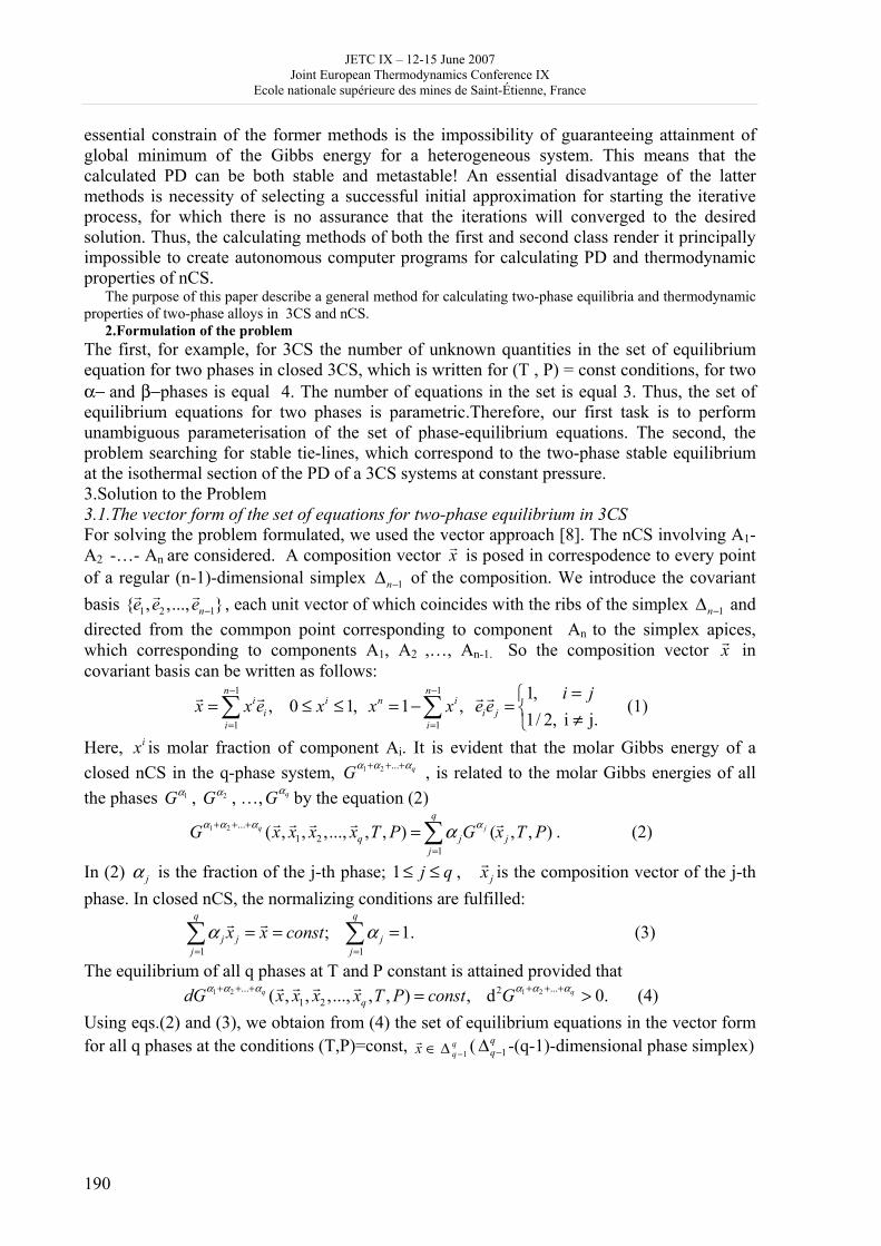
JETC IX – 12-15 June 2007 Joint European Thermodynamics Conference IX
Ecole nationale supérieure des mines de Saint-Étienne, France
190
essential constrain of the former methods is the impossibility of guaranteeing attainment of global minimum of the Gibbs energy for a heterogeneous system. This means that the calculated PD can be both stable and metastable! An essential disadvantage of the latter methods is necessity of selecting a successful initial approximation for starting the iterative process, for which there is no assurance that the iterations will converged to the desired solution. Thus, the calculating methods of both the first and second class render it principally impossible to create autonomous computer programs for calculating PD and thermodynamic properties of nCS.
The purpose of this paper describe a general method for calculating two-phase equilibria and thermodynamic properties of two-phase alloys in 3CS and nCS.
2.Formulation of the problem The first, for example, for 3CS the number of unknown quantities in the set of equilibrium equation for two phases in closed 3CS, which is written for (T , P) = const conditions, for two α− and β−phases is equal 4. The number of equations in the set is equal 3. Thus, the set of equilibrium equations for two phases is parametric.Therefore, our first task is to perform unambiguous parameterisation of the set of phase-equilibrium equations. The second, the problem searching for stable tie-lines, which correspond to the two-phase stable equilibrium at the isothermal section of the PD of a 3CS systems at constant pressure. 3.Solution to the Problem 3.1.The vector form of the set of equations for two-phase equilibrium in 3CS For solving the problem formulated, we used the vector approach [8]. The nCS involving A1- A2 -…- An are considered. A composition vector xr is posed in correspodence to every point of a regular (n-1)-dimensional simplex 1n−Δ of the composition. We introduce the covariant basis 1 2 1{ , ,..., }ne e e −
r r r , each unit vector of which coincides with the ribs of the simplex 1n−Δ and directed from the commpon point corresponding to component An to the simplex apices, which corresponding to components A1, A2 ,…, An-1. So the composition vector xr in covariant basis can be written as follows:
1 1
1 1
1, , 0 1, 1 ,
1/ 2, i j.
n ni i n i
i i ji i
i jx x e x x x e e
− −
= =
=⎧= ≤ ≤ = − = ⎨ ≠⎩∑ ∑r r r r (1)
Here, ix is molar fraction of component Ai. It is evident that the molar Gibbs energy of a closed nCS in the q-phase system, 1 2 ... qGα α α+ + + , is related to the molar Gibbs energies of all the phases 1Gα , 2Gα , …, qGα by the equation (2)
1 2 ...1 2
1( , , ,..., , , ) ( , , )q j
q
q j jj
G x x x x T P G x T Pα α α αα+ + +
=
=∑r r r r r . (2)
In (2) jα is the fraction of the j-th phase; 1 j q≤ ≤ , jxr is the composition vector of the j-th phase. In closed nCS, the normalizing conditions are fulfilled:
1 1; 1.
q q
j j jj j
x x constα α= =
= = =∑ ∑r r (3)
The equilibrium of all q phases at T and P constant is attained provided that 1 2 1 2... ...2
1 2( , , ,..., , , ) , d 0.q qqdG x x x x T P const Gα α α α α α+ + + + + += >r r r r (4)
Using eqs.(2) and (3), we obtaion from (4) the set of equilibrium equations in the vector form for all q phases at the conditions (T,P)=const, 1
qqx −∈ Δr ( 1
qq−Δ -(q-1)-dimensional phase simplex)
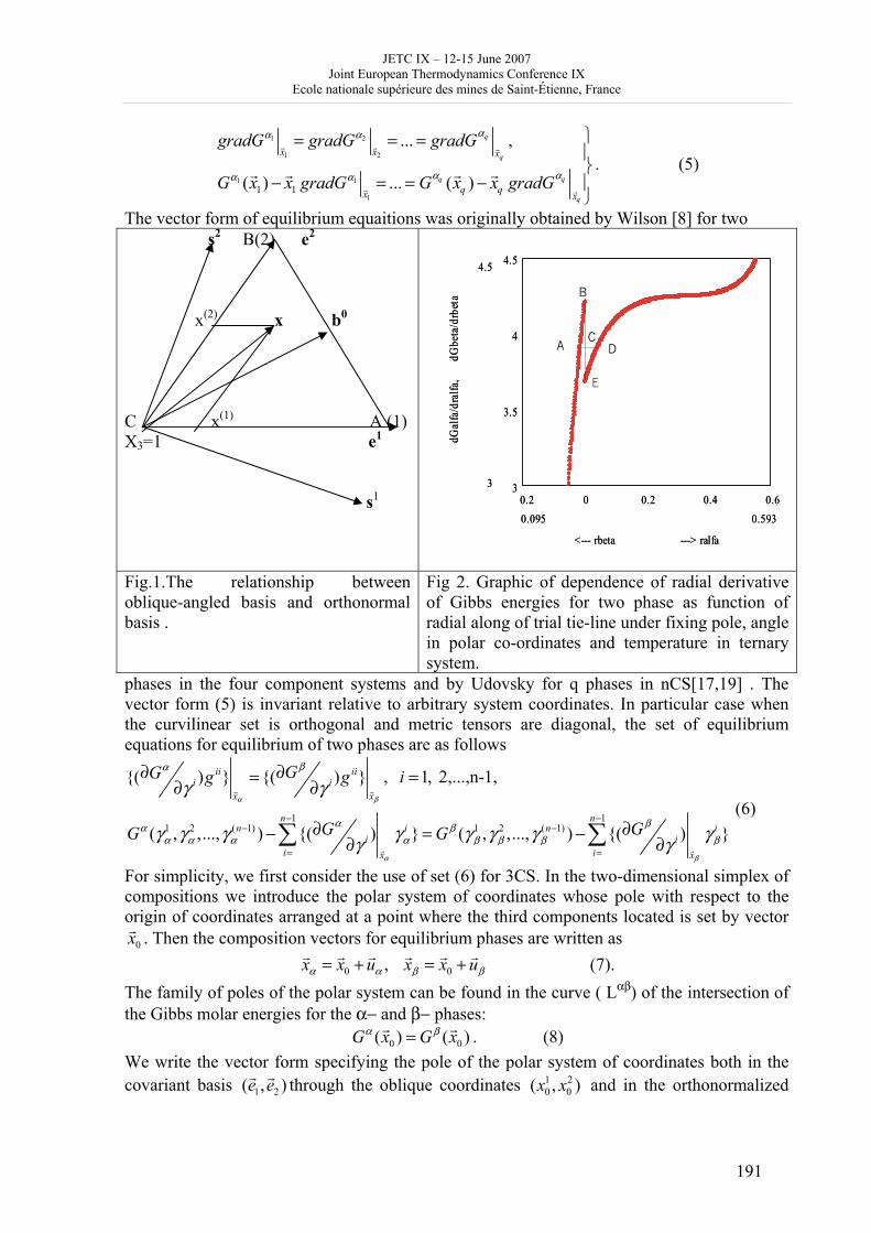
JETC IX – 12-15 June 2007 Joint European Thermodynamics Conference IX
Ecole nationale supérieure des mines de Saint-Étienne, France
191
1 2
1 2
1 1
11 1
... ,
( ) ... ( )
q
q
q q
q
x x x
q qx x
gradG gradG gradG
G x x gradG G x x gradG
αα α
α αα α
⎫= = =⎪⎬
− = = − ⎪⎭
r r r
r r
r r r r . (5)
The vector form of equilibrium equaitions was originally obtained by Wilson [8] for two s2 B(2) e2 x(2) x b0
C x(1) A (1) X3=1 e1 s1
Fig.1.The relationship between oblique-angled basis and orthonormal basis .
Fig 2. Graphic of dependence of radial derivative of Gibbs energies for two phase as function of radial along of trial tie-line under fixing pole, angle in polar co-ordinates and temperature in ternary system.
phases in the four component systems and by Udovsky for q phases in nCS[17,19] . The vector form (5) is invariant relative to arbitrary system coordinates. In particular case when the curvilinear set is orthogonal and metric tensors are diagonal, the set of equilibrium equations for equilibrium of two phases are as follows
1 11 2 ( 1) 1 2 ( 1)
{( ) } {( ) } , 1, 2,...,n-1,
( , ,..., ) {( ) } ( , ,..., ) {( ) }
ii iii i
x x
n nn i n i
i ii ix x
GG g g i
G GG G
α β
α β
βα
α βα βα α α α β β β β
γ γ
γ γ γ γ γ γ γ γγ γ− −
− −
= =
∂ ∂= =∂ ∂
∂ ∂− = −∂ ∂∑ ∑
r r
r r
(6)
For simplicity, we first consider the use of set (6) for 3CS. In the two-dimensional simplex of compositions we introduce the polar system of coordinates whose pole with respect to the origin of coordinates arranged at a point where the third components located is set by vector
0xr . Then the composition vectors for equilibrium phases are written as
0 0, x x u x x uα α β β= + = +r r r r r r (7). The family of poles of the polar system can be found in the curve ( Lαβ) of the intersection of the Gibbs molar energies for the α− and β− phases:
0 0( ) ( )G x G xα β=r r . (8) We write the vector form specifying the pole of the polar system of coordinates both in the covariant basis 1 2( , )e er r through the oblique coordinates 1 2
0 0( , )x x and in the orthonormalized
4.5
3
Ai 1,
0.5930.095 Ai 0,
0.2 0 0.2 0.4 0.63
3.5
4
4.5
<--- rbeta ---> ralfa
dGal
fa/d
ralfa
,
dGbe
ta/d
rbet
a
4.5
3
Ai 1,
0.5930.095 Ai 0,
0.2 0 0.2 0.4 0.63
3.5
4
4.5
<--- rbeta ---> ralfa
dGal
fa/d
ralfa
,
dGbe
ta/d
rbet
a
A
B
CD
JETC IX – 12-15 June 2007 Joint European Thermodynamics Conference IX
Ecole nationale supérieure des mines de Saint-Étienne, France
192
basis 1 2( , )s sr r arranged with respect to oblique basis 1 2( , )e er r so that the bisectrices of angles between the unit vectors of the corresponding bases coincide (see fig.1):
1 2 1 20 0 1 0 2 0 1 0 2x x e x e z s z s= + = +r r r r r . (9)
Fot this case, the polar coordinates of the composition vector for the α− and β− phases completely specify the oblique coordinates of these vectors
1 21 0 2 0
1 21 0 2 0
( cos ) ( sin ),
( cos ) ( sin ), 1, 2.
i i i
i i i
x u r z u r z
x u r z u r z iα α α α α
β β β β β
ϕ ϕϕ ϕ
= + + +
= − + + − + = (10)
Let the pole 1 20 0( , )x x the inside the two-phase (α+β) – field. In this case, with allowance for
the fact that the vectors rαr and rβ
r are antiparallel, set (6) in polar system of coordinates becomes
( , )( , )
( , ) ( , )
( , )
/ /
(1/ ) / (1/ ) /
( ) / ( , ) ( , )
rr
r r
r
G r G r
r G r G
r r G r G r G r
β β αα α
α α β β α
α α
α βϕ π ϕϕ
α βα βϕ ϕ π ϕ
α α βα β α α β β αϕ
ϕ ϕ
ϕ ϕ π ϕ
= +
= +
⎫∂ ∂ = −∂ ∂⎪⎪
∂ ∂ = − ∂ ∂ ⎬⎪⎪+ ∂ ∂ = − = +⎭
(11)
It is worthwhile to divide the process od solution of set (11) into free stages. 1)From equation (8) we find the curve Lαβ,that unambiguously parameterizes the family two-phase tie-lines. In this curve, a pole for polar system coordinates is chosen. 2)We fix a certain value of angle αϕ , then the set of equations (11). Then the subset of equations (11) describe of tentative tie-line, which depends parametrically on i
αϕ and represent the solution to set, which include the first and third equations form set (11). This set two equations is solved using the generalizing
Maxwell “rule of equal areas” in coordinates /G r r∂ ∂ −%where
( , ),( , )=
( , ),
ii
i i
G r r zG r
G r r z
α αβα
α β αββ α
ϕϕ
ϕ π ϕ⎧ ≤⎪⎨
= + ≥⎪⎩%
where r is the modulus of the radius vector directed along the unit vector 0r at angle iαϕ .
3) Then we used method of “angle dichotomy” for calculated stable tie-line as well as calcula calculation of equilibrium values of chemical potentials of components for(α+β)–tie-line. So we calculated all stable (α+β) – tie-line along the curve Lαβ,that unambiguously parame parameterizes the family two-phase tie-lines. These researches have been supported by projects under the terms the NWO-RFBR program (grant 047.014.008), grants 02-03-32621-a and 06-03-33152-a of RFBR References 1.J.W.Gibbs. Thermodynamics. Statistical mechanics.Moscow. Nauka. 1982 (in Russian) 2. U.I.Frankfurt. J.W.Gibbs. The outline of biography. Cit. from [1], p.533-549 (in Russian). 3.J.J.van Laar. Z.für Phys.Chem., 63, 1908,s.216-253; 64, 1909, s.257-297. 4.R.Becker. Ann.der Physik, 32, 1938, s.128-140. 5.B.Ya.Pines. JETPh,13, 1943, N 11-12, p. 411-417 (in Russian) 6.V.I.Danilov, D.S.Kamenetskaya. J.of Phys.Chem. 22, 1948, p.69-79; 81-89 (in Russian). 7.J.L.Mejering. Philips Res. Rep., 3, 1948, p. 281-302. 8.A.J.C.Wilson. Proc. Cambridge Phil.Soc., 37, 1941, p.95-101.
JETC IX – 12-15 June 2007 Joint European Thermodynamics Conference IX
Ecole nationale supérieure des mines de Saint-Étienne, France
193
9. L.S.Palatnik, A.I.Landau.Phase equilibria in multicomponent systems. Kharkov. KhGU, 1961. 10.A.V.Storonkin.Thermodynamics of heterogeneous systems. LGU, Part 1-2, 1967; part 3, 1969. 11.J.C.Wheeler. J. of Chem. Phys., 61, 1974, p.4474-4489. 12.L.Kaufman, H.Bernstein. Computer Calculation of Phase Diagram. Academic Press, New York, 1970. 13. J.F.Counsell, E.B.Less, P.J.Spencer. Met. Sci. J., 5, 1970, p.210-215. 14. H.Gaye, C.H.P.Lupis. Metall. Trans., A 6, 1975, p.1049-1055; 1057-1062. 15. H.L.Lukas, E.Th.Henig, and B.Zimmerman. CALPHAD, 1, 1977, p.225; 1982, p.229 16. B.Sundman, B.Jansson, J.O.Andersson. CALPHAD, 9 1985, p.153- 17. A.L.Udovsky. In: Math.Problems of Chem.Thermodynamics.Nauka.Novosibirsk.1985. P.132-145. 18. A.L.Udovsky,V.N.Karpushkin,E.A.Kozodaeva. CALPHAD, v.19, N 3, 1995, p.245-277. 19. A.L.Udovsky. Doklady of Russian Acad.Sci. v.377, N 6, 2001, p.754-757 (in Russian)
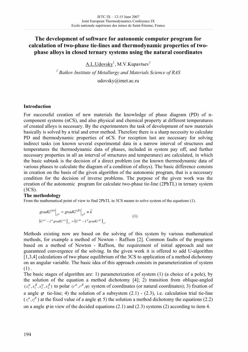
JETC IX – 12-15 June 2007 Joint European Thermodynamics Conference IX
Ecole nationale supérieure des mines de Saint-Étienne, France
194
The development of software for autonomic computer program for calculation of two-phase tie-lines and thermodynamic properties of two-
phase alloys in closed ternary systems using the natural coordinates
A.L.Udovsky1, M.V.Kupavtsev1 1 Baikov Institute of Metallurgy and Materials Science of RAS
Introduction For successful creation of new materials the knowledge of phase diagram (PD) of n-component systems (nCS), and also physical and chemical property at different temperatures of created alloys is necessary. By the experimenters the task of development of new materials basically is solved by a trial and error method. Therefore there is a sharp necessity to calculate PD and thermodynamic properties of nCS. For reception last are necessary for solving indirect tasks (on known several experimental data in a narrow interval of structures and temperatures the thermodynamic data of phases, included in system pay off, and further necessary properties in all an interval of structures and temperature) are calculated, in which the basic subtask is the decision of a direct problem (on the known thermodynamic data of various phases to calculate the diagram of a condition of alloys). The basic difference consists in creation on the basis of the given algorithm of the autonomic program, that is a necessary condition for the decision of inverse problems. The purpose of the given work was the creation of the autonomic program for calculate two-phase tie-line (2PhTL) in ternary system (3CS). The methodology From the mathematical point of view to find 2PhTL in 3CS means to solve system of the equations (1).
kgradGgradGxx
rrr ≡=
βαβα )()(
(1) ( ) ( ) βα
βββαααxx
gradGxGgradGxG rr
rr )()()()( −=− Methods existing now are based on the solving of this system by various mathematical methods, for example a method of Newton - Raffson [2]. Common faults of the programs based on a method of Newton - Raffson, the requirement of initial approach and not guaranteed convergence of the solving. In the given work it is offered to add U-algorithm [1,3,4] calculations of two phase equilibrium of the 3CS to application of a method dichotomy on an angular variable. The basic idea of this approach consists in parameterization of system (1) . The basic stages of algorithm are: 1) parameterization of system (1) (a choice of a pole), by the solution of the equation a method dichotomy [4]; 2) transition from oblique-angled
),,,( 2211βαβα xxxx to polar ),,( ϕβα rr system of coordinates (or natural coordinates); 3) fixation of
a angle ϕ tie-line; 4) the solution of a subsystem (2.1) - (2.3), i.e. calculation trial tie-line ( βα
ii rr , ) at the fixed value of a angle ϕ; 5) the solution a method dichotomy the equations (2.2) on a angle ϕ in view of the decided equations (2.1) and (2.3) systems (2) according to item 4.
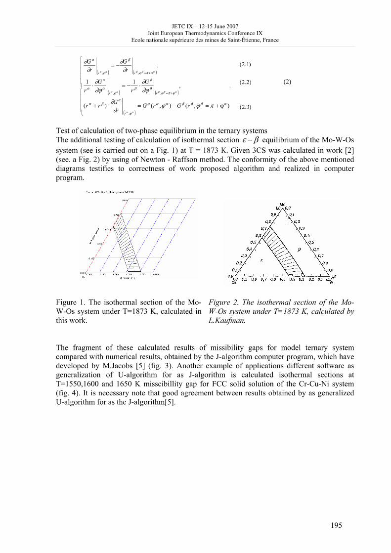
JETC IX – 12-15 June 2007 Joint European Thermodynamics Conference IX
Ecole nationale supérieure des mines de Saint-Étienne, France
195
( ) ( )
( ) ( )
( ))3.2(
)2.2(
)1.2(
.
),(),()(
,11
,
,
,,
,,
⎪⎪⎪⎪
⎩
⎪⎪⎪⎪
⎨
⎧
ϕ+=−=⋅+
⋅−=⋅
−=
ϕ+=
ϕ+=
αβββααα
ϕ
αβα
πϕβ
β
βϕ
α
α
α
πϕ
β
ϕ
α
πϕϕ∂
∂
∂ϕ∂
∂ϕ∂
∂∂
∂∂
αα
αββαα
αββαα
rGrGr
Grr
Gr
Gr
rG
rG
r
rr
rr
(2)
Test of calculation of two-phase equilibrium in the ternary systems The additional testing of calculation of isothermal section ε β− equilibrium of the Mo-W-Os system (see is carried out on a Fig. 1) at Т = 1873 К. Given 3CS was calculated in work [2] (see. a Fig. 2) by using of Newton - Raffson method. The conformity of the above mentioned diagrams testifies to correctness of work proposed algorithm and realized in computer program.
Figure 1. The isothermal section of the Mo-W-Os system under T=1873 K, calculated in this work.
Figure 2. The isothermal section of the Mo-W-Os system under T=1873 K, calculated by L.Kaufman.
The fragment of these calculated results of missibility gaps for model ternary system compared with numerical results, obtained by the J-algorithm computer program, which have developed by M.Jacobs [5] (fig. 3). Another example of applications different software as generalization of U-algorithm for as J-algorithm is calculated isothermal sections at T=1550,1600 and 1650 K misscibillity gap for FCC solid solution of the Cr-Cu-Ni system (fig. 4). It is necessary note that good agreement between results obtained by as generalized U-algorithm for as the J-algorithm[5].
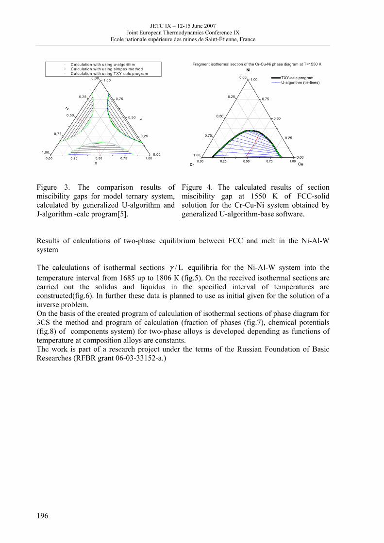
JETC IX – 12-15 June 2007 Joint European Thermodynamics Conference IX
Ecole nationale supérieure des mines de Saint-Étienne, France
196
0,00 0,25 0,50 0,75 1,00
0,00
0,25
0,50
0,75
1,00 0,00
0,25
0,50
0,75
1,00
Y
Calculation w ith using u-algorithm Calculation w ith using sim pex m ethod Calculation w ith using TXY-calc program
Z
X
0.00 0.25 0.50 0.75 1.00
0.00
0.25
0.50
0.75
1.00 0.00
0.25
0.50
0.75
1.00 TXY-calc program U-algorithm (tie-lines)
Fragment isothermal section of the Cr-Cu-Ni phase diagram at T=1550 K
Cr
Ni
Cu
Figure 3. The comparison results of miscibility gaps for model ternary system, calculated by generalized U-algorithm and J-algorithm -calc program[5].
Figure 4. The calculated results of section miscibility gap at 1550 K of FCC-solid solution for the Cr-Cu-Ni system obtained by generalized U-algorithm-base software.
Results of calculations of two-phase equilibrium between FCC and melt in the Ni-Al-W system The calculations of isothermal sections / Lγ equilibria for the Ni-Al-W system into the temperature interval from 1685 up to 1806 К (fig.5). On the received isothermal sections are carried out the solidus and liquidus in the specified interval of temperatures are constructed(fig.6). In further these data is planned to use as initial given for the solution of a inverse problem. On the basis of the created program of calculation of isothermal sections of phase diagram for 3CS the method and program of calculation (fraction of phases (fig.7), chemical potentials (fig.8) of components system) for two-phase alloys is developed depending as functions of temperature at composition alloys are constants. The work is part of a research project under the terms of the Russian Foundation of Basic Researches (RFBR grant 06-03-33152-а.)
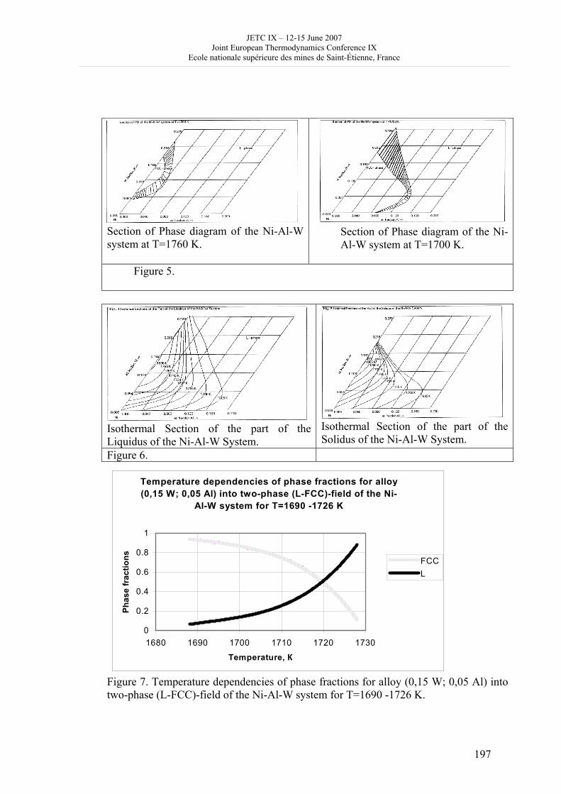
JETC IX – 12-15 June 2007 Joint European Thermodynamics Conference IX
Ecole nationale supérieure des mines de Saint-Étienne, France
197
Section of Phase diagram of the Ni-Al-W system at T=1760 K.
Section of Phase diagram of the Ni-Al-W system at T=1700 K.
Figure 5.
Isothermal Section of the part of the Liquidus of the Ni-Al-W System.
Isothermal Section of the part of the Solidus of the Ni-Al-W System.
Figure 6.
Figure 7. Temperature dependencies of phase fractions for alloy (0,15 W; 0,05 Al) into two-phase (L-FCC)-field of the Ni-Al-W system for T=1690 -1726 K.
Temperature dependencies of phase fractions for alloy (0,15 W; 0,05 Al) into two-phase (L-FCC)-field of the Ni-
Al-W system for T=1690 -1726 K
0
0.2
0.4
0.6
0.8
1
1680 1690 1700 1710 1720 1730
Temperature, К
Phas
e fr
actio
ns FCCL
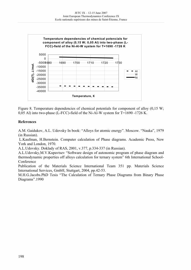
JETC IX – 12-15 June 2007 Joint European Thermodynamics Conference IX
Ecole nationale supérieure des mines de Saint-Étienne, France
198
Figure 8. Temperature dependencies of chemical potentials for component of alloy (0,15 W; 0,05 Al) into two-phase (L-FCC)-field of the Ni-Al-W system for T=1690 -1726 K. References A.M. Gaidukov, A.L. Udovsky In book: “Alloys for atomic energy”. Мoscow. “Nauka”, 1979 (in Russian). L.Kaufman, H.Bernstein. Computer calculation of Phase diagrams. Academic Press, New York and London, 1970. A.L.Udovsky. Doklady of RAS, 2001, v.377, p.334-337 (in Russian). A.L.Udovsky,M.V.Kupavtsev “Software design of autonomic program of phase diagram and thermodynamic properties off alloys calculation for ternary system” 6th International School-Conference Publication of the Materials Science International Team 351 pp. Materials Science International Services, GmbH, Stuttgart, 2004, pp.42-53. M.H.G.Jacobs.PhD Tesis “The Calculation of Ternary Phase Diagrams from Binary Phase Diagrams”.1990
Temperature dependencies of chemical potencials for component of alloy (0,15 W; 0,05 Al) into two-phase (L-
FCC)-field of the Ni-Al-W system for T=1690 -1726 K
-40000-35000-30000-25000-20000-15000-10000
-50000
5000
1680 1690 1700 1710 1720 1730
Temperature, К
dGi(T
), J.
/mol
.
AlWNi
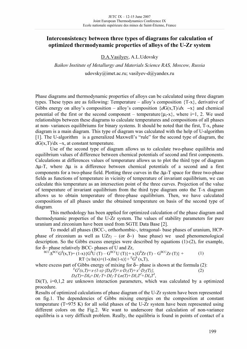
JETC IX – 12-15 June 2007 Joint European Thermodynamics Conference IX
Ecole nationale supérieure des mines de Saint-Étienne, France
199
Interconsistency between three types of diagrams for calculation of optimized thermodynamic properties of alloys of the U-Zr system
D.A.Vasilyev, A.L.Udovsky
Baikov Institute of Metallurgy and Materials Science RAS, Moscow, Russia
[email protected]; [email protected] Phase diagrams and thermodynamic properties of alloys can be calculated using three diagram types. These types are as following: Temperature – alloy’s composition {T-x}, derivative of Gibbs energy on alloy’s composition – alloy’s composition {dG(x,T)/dx −x} and chemical potential of the first or the second component – temperature{μi-x}, where i=1, 2. We used relationships between these diagrams to calculate temperatures and compositions of all phases at non- variances equilibriums for binary systems. It should be noted that the first, T-x, phase diagram is a main diagram. This type of diagram was calculated with the help of U-algorithm [1]. The U-algorithm is a generalized Maxwell’s “rule” for the second type of diagram, the dG(x,T)/dx −x, at constant temperature.
Use of the second type of diagram allows us to calculate two-phase equilibria and equilibrium values of difference between chemical potentials of second and first components. Calculations at differences values of temperature allows us to plot the third type of diagram Δμ-T, where Δμ is a difference between chemical potentials of a second and a first components for a two-phase field. Plotting three curves in the Δμ-T space for three two-phase fields as functions of temperature in vicinity of temperature of invariant equilibrium, we can calculate this temperature as an intersection point of the three curves. Projection of the value of temperature of invariant equilibrium from the third type diagram onto the T-x diagram allows us to obtain temperature of three-phase equilibrium. Then, we have calculated compositions of all phases under the obtained temperature on basis of the second type of diagram.
This methodology has been applied for optimized calculation of the phase diagram and thermodynamic properties of the U-Zr system. The values of stability parameters for pure uranium and zirconium have been used from SGTE Data Base [2].
To model all phases (BCC-, orthorhombic-, tetragonal- base phases of uranium, HCP-phase of zirconium as well as UZr2 – (or δ−) base phase) we used phenomenological description. So the Gibbs excess energies were described by equations (1)-(2), for example, for δ− phase relatively BCC- phases of U and Zr,
BCCΔBCCGδ(x,T)= (1-x){GδU (T) – GBCCU (T)}+ x{GδZr (T) – GBCCZr (T)} + RT·{x·ln(x)+(1-x)ln(1-x)}+ EGδ (x,T),
(1)
where excess part of Gibbs energy of mixing for δ− phase is shown at the formula (2): EGδ(x,T)=x·(1-x)·{D0(T)+x·D1(T)+x2·D2(T)},
DI(T)=DI0+DI1·T+DI2·T·Ln(T)+DI3T2+DI4T3, (2)
Di(T), i=0,1,2 are unknown interaction parameters, which was calculated by а optimized procedure. Results of optimized calculations of phase diagram of the U-Zr system have been represented on fig.1. The dependencies of Gibbs mixing energies on the composition at constant temperature (T=975 K) for all solid phases of the U-Zr system have been represented using different colors on the Fig.2. We want to underscore that calculation of non-variance equilibria is a very difficult problem. Really, the equilibria is found in points of contact of a
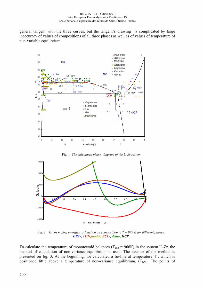
JETC IX – 12-15 June 2007 Joint European Thermodynamics Conference IX
Ecole nationale supérieure des mines de Saint-Étienne, France
200
general tangent with the three curves, but the tangent’s drawing is complicated by large inaccuracy of values of compositions of all three phases as well as of values of temperature of non-variable equilibrium.
Fig. 1 The calculated phase diagram of the U-Zr system
-2000
-1000
0
1000
2000
3000
0 0.1 0.2 0.3 0.4 0.5 0.6 0.7 0.8 0.9 1
x, mole fraction Zr
G, j
oule
Fig. 2 Gibbs mixing energies as function on composition at T = 975 K for different phases:
ORT-, TET-,liquid-, BCC-, delta-, HCP.
To calculate the temperature of monotectoid balances (Texp = 966К) in the system U-Zr, the method of calculation of non-variance equilibrium is used. The essence of the method is presented on fig. 3. At the beginning, we calculated a tie-line at temperature T1, which is positioned little above a temperature of non-variance equilibrium, (TNV). The points of
600
650
700
750
800
850
900
950
1000
1050
1100
1150
0 0,1 0,2 0,3 0,4 0,5 0,6 0,7 0,8 0,9 1
U x, mole fraction(Zr) Zr
T, K
BCC
δ
ORT + δ
ORT + BCC'
TET + BCC'
δ + HCP
BCC'
BCC' + HCP
963,54 K
935 K
889,96 K 886 K
ORT
TETδ + BCC'
TET + BCC
BCC + BCC'
0,719 0,724
0,74
0,802
0,588
0,4520,155
0,28 997 K
0,025
0,99998
▲ 54Sum tet+bccΔ 58Duf one phase◊ 57Phi ZrV Arkl■ 62Zeg two phase♦ 62Zeg one phase♦ 54Sum ort+bcc♦ 54Sum tet
● 62Zeg three phase◊ 54Sum two phase♦ 92 Aka□ 58How▲ 54Sum bcc+hcp
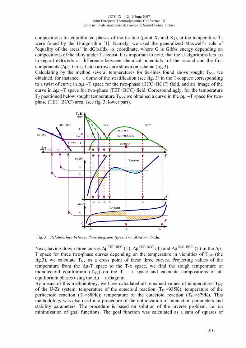
JETC IX – 12-15 June 2007 Joint European Thermodynamics Conference IX
Ecole nationale supérieure des mines de Saint-Étienne, France
201
compositions for equilibrated phases of the tie-line (point X3 and X4), at the temperature T1 were found by the U-algorithm [1]. Namely, we used the generalized Maxwell’s rule of "equality of the areas" in dG(x)/dx –x coordinate, where G is Gibbs energy depending on compositions of the alloy under T1=const. It is important to note, that the U-algorithms lets us to regard dG(x)/dx as difference between chemical potentials of the second and the first components (Δμ). Cross-hatch arrows are shown on scheme (fig.3). Calculating by the method several temperatures for tie-lines found above sought TNV, we obtained, for instance, a dome of the stratification (see fig. 3) in the T-x space corresponding to a twist of curve in Δμ −T space for the two-phase (BCC+BCC') field, and an image of the curve in Δμ −T space for two-phase (TET+BCC) field. Correspondingly, for the temperature T2 positioned below sought temperature TNV, we obtained a curve in the Δμ −T space for two-phase (TET+BCC') area, (see fig. 3, lower part).
Fig. 3 Relationships between three diagrams types: T–x, dG/dx–x, T–Δµ. Next, having drawn three curves ΔμTET+BCC (T), ΔμTET+BCC' (T) and ΔμBCC+BCC' (T) in the Δμ-T space for three two-phase curves depending on the temperature in vicinities of TNV (the fig.3), we calculate TNV as a cross point of these three curves. Projecting values of the temperature from the Δμ-T space to the T-x space, we find the sough temperature of monotectoid equilibrium (TNV) on the T – x space and calculate compositions of all equilibrium phases using the Δμ − x diagram. By means of this methodology, we have calculated all remained values of temperatures TNV of the U-Zr system: temperature of the eutectoid reaction (TE1=935K); temperature of the peritectoid reaction (TP=889K); temperature of the eutectoid reaction (TE2=879K). This methodology was also used in a procedure of the optimization of interaction parameters and stability parameters. The procedure is based on solution of the inverse problem, i.e. on minimization of goal functions. The goal function was calculated as a sum of squares of
T, K
dG/dX
X
Δµ 0
0
1049
TNV
X
BCC BCC’
β-U
T1
X1 X2 X3 X4 Z1
X1 X2 X3 X4 Z1
K2
K1
K2 K1
BCC+BCC’
βU+BCC
dG/dX
0 X
X5 Z2 X6
K3
K3
T2 βU+BCC’
BCC+BCC’
βU+BCC’
TNV=963,54K
T1=const
T2=const
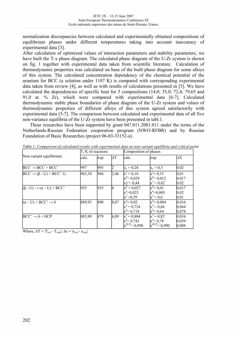
JETC IX – 12-15 June 2007 Joint European Thermodynamics Conference IX
Ecole nationale supérieure des mines de Saint-Étienne, France
202
normalization discrepancies between calculated and experimentally obtained compositions of equilibrium phases under different temperatures taking into account inaccuracy of experimental data [3]. After calculation of optimized values of interaction parameters and stability parameters, we have built the T-x phase diagram. The calculated phase diagram of the U-Zr system is shown on fig. 1 together with experimental data taken from scientific literature. Calculation of thermodynamic properties was calculated on base of the built phase diagram for some alloys of this system. The calculated concentration dependency of the chemical potential of the uranium for BCC (a solution under 1107 K) is compared with corresponding experimental data taken from review [4], as well as with results of calculations presented in [5]. We have calculated the dependencies of specific heat for 5 compositions (14,0; 35,0; 72,4; 79,65 and 91,0 at. % Zr), which were compared with experimental data [6-7]. Calculated thermodynamic stable phase boundaries of phase diagram of the U-Zr system and values of thermodynamic properties of different alloys of this system agreed satisfactorily with experimental data [5-7]. The comparison between calculated and experimental data of all five non-variance equilibria of the U-Zr system have been presented in tabl.1.
These researches have been supported by grant 047.011.2001.011 under the terms of the Netherlands-Russian Federation cooperation program (NWO-RFBR) and by Russian Foundation of Basic Researches (project 06-03-33152-a). Table 1. Comparison of calculated results with experimental data on non-variant equilibria and critical point
T, K of reactions Composition of phases Non-variant equilibrium calc. exp. ∆T calc. exp. ∆X
BCC → BCC + BCC’ 997 995 2 xc = 0,28 xc = 0,3 0,02 BCC → (β - U) + BCC’ 1) 963,54 966 2,46 xγ = 0,16
xβ= 0,029 xγ’= 0,44
xγ= 0,15 xβ= 0,012 xγ’= 0,42
0,01 0,017 0.02
(β - U) → (α – U) + BCC’ 935 935 0 xβ = 0,027 xα=0,025 xγ’=0,59
xβ= 0,01 xα=0,005 xγ’= 0,6
0,017 0,02 0,01
(α – U) + BCC’ → δ 889,93 890 0,07 xα= 0,02 xγ’= 0,724 xδ= 0,718
xα= 0,004 xγ’= 0,66 xδ= 0,64
0,016 0,064 0,078
BCC’ → δ + HCP 885,89 879 6,89 xγ’= 0,804 xδ= 0,741 xHCP= 0,998
xγ’= 0,82 xδ= 0,78 xHCP= 0,990
0,016 0,039 0,008
Where, ∆T = |Tcal - Texp|; ∆x = |xcal - xexp|
JETC IX – 12-15 June 2007 Joint European Thermodynamics Conference IX
Ecole nationale supérieure des mines de Saint-Étienne, France
203
1.A.T.Dinsdale. SGTE DATA FOR PURE ELEMENTS .CALPHAD, 1991, v. 15, № 4, P.317-425. 2. A.L.Udovsky. Izvestiya AN USSR, Metally. 1990, № 2, p.136-158 (in Russian). 3. A.L.Udovsky. The Physical bases of computer design of materials. Great Novgorod. 2005 (in Russian). 4. R.I.Sheldon, D.E.Peterson. The U-Zr (Uranium-Zirconium) System. Los Alamos National Laboratory. Bulletin of Alloys Phase Diagrams. Vol. 10. 1989. № 2. P. 165-181. 5. P.-Y.Chevalier, E.Fisher, B.Cheynet. Progress in the Thermodynamic modeling of the O-U-Zr ternary system. CALPHAD, 2004, v. 28, p.15-40. 6. Y.Takahashi, K.Yamamoto, T.Ohsato, H.Shimada, T. Terai. J. Nuclear Materials, 1989, v.167, p.147-151. 7.B-H.Lee et all. J.Nucl. Materials. 2007, v.360, p.315-320.
JETC IX – 12-15 June 2007 Joint European Thermodynamics Conference IX
Ecole nationale supérieure des mines de Saint-Étienne, France
204
Before thermodynamics: a short history of the steam engine
Thierry Veyron
Ville de Saint-Etienne, 42000, France
[email protected] Before, well before thermodynamics was founded as a science in the first half of the nineteenth century, technicians had foreseen and even used the driving power of fire: one remembers the eolipylon designed by Heron of Alexandria, in the first century of our era; then, following the example of the Greek mechanic, similar machines were built by the engineers of the Renaissance, notably Salomon de Caus. These machines remained “thaumata”, literally wonders, or even miracles. They also attested what anthropologist Claude lévi-strauss names “handyman thinking”. Nevertheless, they correspond to a step in the reflection of scholars such as Papin and Savery, who succeeded in foreseeing true industrial devices thanks to the use of steam, or atmosphere pressure, that was evidenced by Pascal and Torricelli in the years 1640. The classical science comes into play. In 1690, Denis Papin presents his pneumatic cylinder. The device is a simple cylinder-piston set in which one pours water before putting it on the fire, which provokes the rising of the piston, maintained in high position by a wedge that it suffices to withdraw, after cooling and condensation, to release the force of the atmospheric pressure on the full height of the cylinder. In 1698, Thomas Savery designs a fire engine, aimed to pump the water out of the mines, that uses the vacuum and the atmospheric pressure to suck out water, and the steam pressure to repel it. Their ideas are made practical by Thomas Newcomen, a blacksmith from Devonshire: he personifies the return to handyman thinking! His atmospheric machine uses the steam produced in a boiler and admitted in a cylinder then condensed in order to obtain vacuum and to release the action of the atmosphere: this is this very force that drives the pump. The machine of Newcomen dates back to 1705. It very quickly spreads across Great Britain: pumping water from the mines, filling the canals, supplying drinkable water to the cities. However, it is very slow and cannot offer a rotation movement. It comes back to James Watt to design the classical steam engine. Watt is a practical scholar, a worker philosopher according to the word of chemist Robison. Undertaking the critical assessment of the atmospheric machine, he notes the huge heat loss caused by condensation inside the cylinder and concludes to the superiority of the driving force provided by steam; the condenser is separated from the cylinder, which is itself isolated so that its high temperature is preserved. Such is the steam engine, with simple effect, from Watt, still used to pumping (1769). Watt then conceives the so-called rotation machine, i.e. a double effect machine where steam acts on both faces of the piston, allowing a quick movement and therefore the achievement of a circular movement, by the addition to the rod of a crank and of a wheel (1783) : the steam engine then permits all industrial uses, provided the fluid pressure is

JETC IX – 12-15 June 2007 Joint European Thermodynamics Conference IX
Ecole nationale supérieure des mines de Saint-Étienne, France
205
allowed to vary (high pressure locomotives or mining extraction machines, without condenser) and relax (Woolf machines with double expansion, marine machines). The steam engine is perfectly established at the end of the eighteenth century. Associated with other inventions and innovations in the domains of textile, metallurgy, mine working, it gives Great Britain a considerable advance over the other developed nations, especially France, that enters at the same moment in the revolutionary tempest
JETC IX – 12-15 June 2007 Joint European Thermodynamics Conference IX
Ecole nationale supérieure des mines de Saint-Étienne, France
206
Thermal diffusion of neutral and charged colloidal dispersions
Simone Wiegand, Hui Ning, Johan Buitenhuis, Jan K.G. Dhont
IFF-Soft condensed mater, Research Center Jülich, Leo-Brandt Str., 52428 Jülich
[email protected] Introduction Colloidal particles show many physical phenomena that are also found in ordinary molecular systems. Consequently, colloids have been used frequently to study fundamental questions in physics. Therefore, it is expected that they are also a suitable model system to illuminate the microscopic mechanism underlying the Ludwig-Soret effect, which was discovered already 150 years ago [1, 2]. This effect, also known as thermal diffusion, describes the diffusive mass transport induced by a temperature gradient in a multi-component system. A number of studies show that interactions play an important role for the thermal diffusion behavior, where long ranged repulsion between charged micelles and colloids has been considered [3-5]. Conceptually, thermal diffusive behavior of highly diluted and concentrated dispersions can be differentiated [6]. In dilute dispersions, where colloid-colloid interactions can be neglected, the thermal diffusion coefficient of the colloids is determined by the nature of the interactions between single colloidal particles and solvent molecules (and possibly other solutes like ions that form a double layer around the colloids). Structural changes of the surrounding solvation layer due to temperature changes and/or changes of the solvent composition may induce a sign change of the thermal diffusive behavior of single colloidal particles. Usually, the mechanism leading to a sign change is system dependent. Although, for several aqueous mixtures with and without solutes such as polymers and colloids, we found the sign change concentration is almost system independent and strongly correlated with the breakdown of the hydrogen-bond network [6]. Also the temperature dependence of ST for a large class of macromolecules and colloids in water shows a distinctive universal characteristic [7]. A pronounced concentration dependence of the Soret coefficient has been found in experiments [4, 8] and is predicted by theory [9, 10]. In recent years, modern optical techniques have been developed which allow the investigation of complex fluids with slow dynamics such as polymer solutions and blends, micellar solutions, colloidal dispersions and bio-molecules [5, 7, 11-14]. The main issues of interest were the derivation of scaling laws and to understand the sign change of the Soret coefficient for macromolecular and colloidal systems on the basis of existing theories for molecular fluids. In the past few years several theoretical concepts have been proposed to understand single particle and colloid-colloid interaction contributions to the thermophoretic motion of colloidal particles [9, 10, 15-17]. While the majority of the theoretical approaches give expressions for the single particle contribution, the work by Dhont gives explicit expressions for the contribution of colloid-colloid interactions to the thermal diffusion coefficient DT. These interaction contributions lead to a concentration dependence of the thermal diffusion coefficient. According to this theory, a sign change of the Soret coefficient as a function of temperature and concentration is possible for appropriate interaction parameters. In a recent work Dhont et al. [18] derived an expression for the single-particle thermal diffusion coefficient of a charged colloidal sphere on the basis of a force balance on the Brownian time scale in combination with thermodynamics. The goal of this
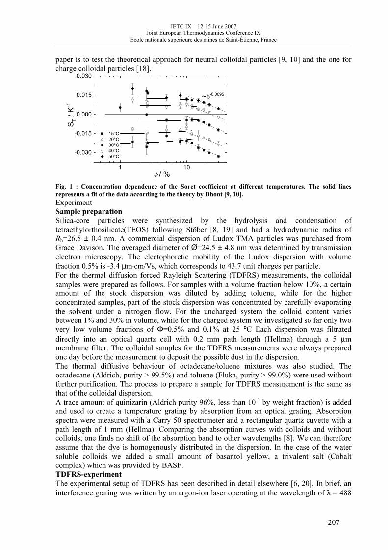
JETC IX – 12-15 June 2007 Joint European Thermodynamics Conference IX
Ecole nationale supérieure des mines de Saint-Étienne, France
207
paper is to test the theoretical approach for neutral colloidal particles [9, 10] and the one for charge colloidal particles [18].
1 10
-0.030
-0.015
0.000
0.015
0.030
S T / K
-1
φ / %
~φ-0.0095
15°C 20°C 30°C 40°C 50°C
Fig. 1 : Concentration dependence of the Soret coefficient at different temperatures. The solid lines represents a fit of the data according to the theory by Dhont [9, 10]. Experiment Sample preparation Silica-core particles were synthesized by the hydrolysis and condensation of tetraethylorthosilicate(TEOS) following Stöber [8, 19] and had a hydrodynamic radius of Rh=26.5 ± 0.4 nm. A commercial dispersion of Ludox TMA particles was purchased from Grace Davison. The averaged diameter of Ø=24.5 ± 4.8 nm was determined by transmission electron microscopy. The electophoretic mobility of the Ludox dispersion with volume fraction 0.5% is -3.4 μm⋅cm/Vs, which corresponds to 43.7 unit charges per particle. For the thermal diffusion forced Rayleigh Scattering (TDFRS) measurements, the colloidal samples were prepared as follows. For samples with a volume fraction below 10%, a certain amount of the stock dispersion was diluted by adding toluene, while for the higher concentrated samples, part of the stock dispersion was concentrated by carefully evaporating the solvent under a nitrogen flow. For the uncharged system the colloid content varies between 1% and 30% in volume, while for the charged system we investigated so far only two very low volume fractions of Φ=0.5% and 0.1% at 25 ºC Each dispersion was filtrated directly into an optical quartz cell with 0.2 mm path length (Hellma) through a 5 μm membrane filter. The colloidal samples for the TDFRS measurements were always prepared one day before the measurement to deposit the possible dust in the dispersion. The thermal diffusive behaviour of octadecane/toluene mixtures was also studied. The octadecane (Aldrich, purity > 99.5%) and toluene (Fluka, purity > 99.0%) were used without further purification. The process to prepare a sample for TDFRS measurement is the same as that of the colloidal dispersion. A trace amount of quinizarin (Aldrich purity 96%, less than 10-4 by weight fraction) is added and used to create a temperature grating by absorption from an optical grating. Absorption spectra were measured with a Carry 50 spectrometer and a rectangular quartz cuvette with a path length of 1 mm (Hellma). Comparing the absorption curves with colloids and without colloids, one finds no shift of the absorption band to other wavelengths [8]. We can therefore assume that the dye is homogenously distributed in the dispersion. In the case of the water soluble colloids we added a small amount of basantol yellow, a trivalent salt (Cobalt complex) which was provided by BASF. TDFRS-experiment The experimental setup of TDFRS has been described in detail elsewhere [6, 20]. In brief, an interference grating was written by an argon-ion laser operating at the wavelength of λ = 488
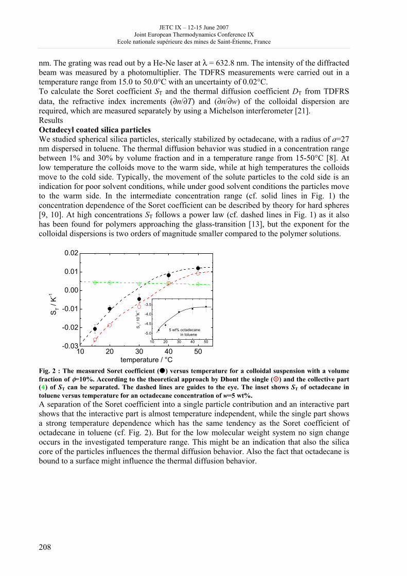
JETC IX – 12-15 June 2007 Joint European Thermodynamics Conference IX
Ecole nationale supérieure des mines de Saint-Étienne, France
208
nm. The grating was read out by a He-Ne laser at λ = 632.8 nm. The intensity of the diffracted beam was measured by a photomultiplier. The TDFRS measurements were carried out in a temperature range from 15.0 to 50.0°C with an uncertainty of 0.02°C. To calculate the Soret coefficient ST and the thermal diffusion coefficient DT from TDFRS data, the refractive index increments (∂n/∂T) and (∂n/∂w) of the colloidal dispersion are required, which are measured separately by using a Michelson interferometer [21]. Results Octadecyl coated silica particles We studied spherical silica particles, sterically stabilized by octadecane, with a radius of a=27 nm dispersed in toluene. The thermal diffusion behavior was studied in a concentration range between 1% and 30% by volume fraction and in a temperature range from 15-50°C [8]. At low temperature the colloids move to the warm side, while at high temperatures the colloids move to the cold side. Typically, the movement of the solute particles to the cold side is an indication for poor solvent conditions, while under good solvent conditions the particles move to the warm side. In the intermediate concentration range (cf. solid lines in Fig. 1) the concentration dependence of the Soret coefficient can be described by theory for hard spheres [9, 10]. At high concentrations ST follows a power law (cf. dashed lines in Fig. 1) as it also has been found for polymers approaching the glass-transition [13], but the exponent for the colloidal dispersions is two orders of magnitude smaller compared to the polymer solutions.
10 20 30 40 50-0.03
-0.02
-0.01
0.00
0.01
0.02
10 20 30 40 50
-5.0
-4.5
-4.0
-3.5
S T / K-1
temperature / °C
5 wt% octadecane in toluene
ST /
10-3K
-1
Fig. 2 : The measured Soret coefficient ( ) versus temperature for a colloidal suspension with a volume fraction of φ=10%. According to the theoretical approach by Dhont the single ( ) and the collective part (4) of ST can be separated. The dashed lines are guides to the eye. The inset shows ST of octadecane in toluene versus temperature for an octadecane concentration of w=5 wt%. A separation of the Soret coefficient into a single particle contribution and an interactive part shows that the interactive part is almost temperature independent, while the single part shows a strong temperature dependence which has the same tendency as the Soret coefficient of octadecane in toluene (cf. Fig. 2). But for the low molecular weight system no sign change occurs in the investigated temperature range. This might be an indication that also the silica core of the particles influences the thermal diffusion behavior. Also the fact that octadecane is bound to a surface might influence the thermal diffusion behavior.
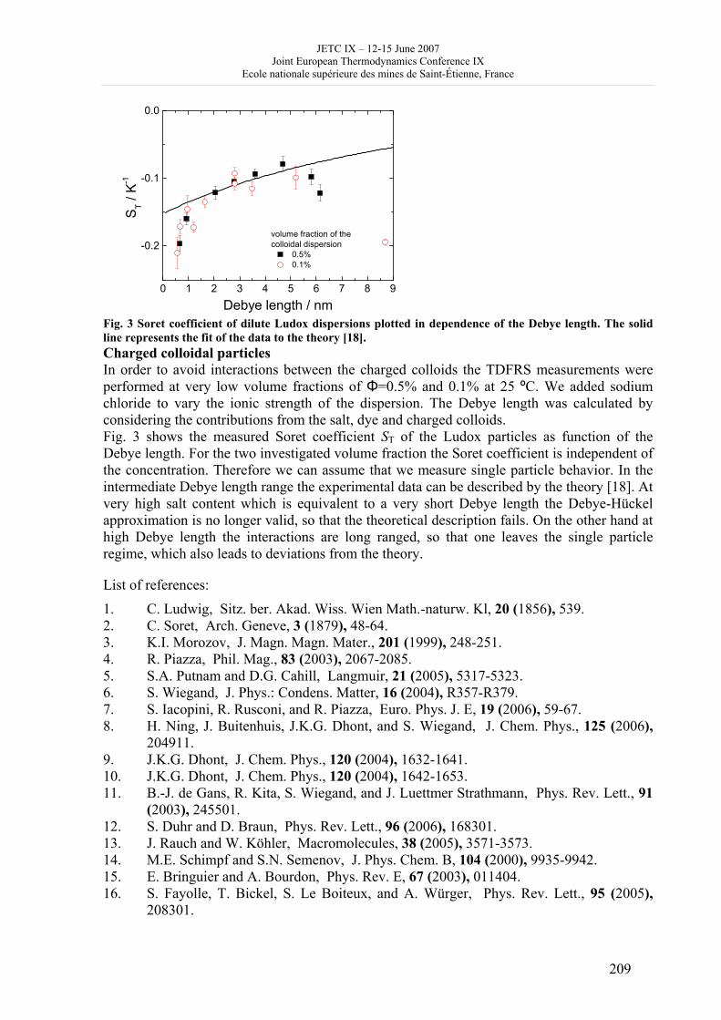
JETC IX – 12-15 June 2007 Joint European Thermodynamics Conference IX
Ecole nationale supérieure des mines de Saint-Étienne, France
209
0 1 2 3 4 5 6 7 8 9
-0.2
-0.1
0.0
volume fraction of the colloidal dispersion
0.5% 0.1%
ST /
K-1
Debye length / nm Fig. 3 Soret coefficient of dilute Ludox dispersions plotted in dependence of the Debye length. The solid line represents the fit of the data to the theory [18]. Charged colloidal particles In order to avoid interactions between the charged colloids the TDFRS measurements were performed at very low volume fractions of Φ=0.5% and 0.1% at 25 ºC. We added sodium chloride to vary the ionic strength of the dispersion. The Debye length was calculated by considering the contributions from the salt, dye and charged colloids. Fig. 3 shows the measured Soret coefficient ST of the Ludox particles as function of the Debye length. For the two investigated volume fraction the Soret coefficient is independent of the concentration. Therefore we can assume that we measure single particle behavior. In the intermediate Debye length range the experimental data can be described by the theory [18]. At very high salt content which is equivalent to a very short Debye length the Debye-Hückel approximation is no longer valid, so that the theoretical description fails. On the other hand at high Debye length the interactions are long ranged, so that one leaves the single particle regime, which also leads to deviations from the theory.
List of references:
1. C. Ludwig, Sitz. ber. Akad. Wiss. Wien Math.-naturw. Kl, 20 (1856), 539. 2. C. Soret, Arch. Geneve, 3 (1879), 48-64. 3. K.I. Morozov, J. Magn. Magn. Mater., 201 (1999), 248-251. 4. R. Piazza, Phil. Mag., 83 (2003), 2067-2085. 5. S.A. Putnam and D.G. Cahill, Langmuir, 21 (2005), 5317-5323. 6. S. Wiegand, J. Phys.: Condens. Matter, 16 (2004), R357-R379. 7. S. Iacopini, R. Rusconi, and R. Piazza, Euro. Phys. J. E, 19 (2006), 59-67. 8. H. Ning, J. Buitenhuis, J.K.G. Dhont, and S. Wiegand, J. Chem. Phys., 125 (2006),
204911. 9. J.K.G. Dhont, J. Chem. Phys., 120 (2004), 1632-1641. 10. J.K.G. Dhont, J. Chem. Phys., 120 (2004), 1642-1653. 11. B.-J. de Gans, R. Kita, S. Wiegand, and J. Luettmer Strathmann, Phys. Rev. Lett., 91
(2003), 245501. 12. S. Duhr and D. Braun, Phys. Rev. Lett., 96 (2006), 168301. 13. J. Rauch and W. Köhler, Macromolecules, 38 (2005), 3571-3573. 14. M.E. Schimpf and S.N. Semenov, J. Phys. Chem. B, 104 (2000), 9935-9942. 15. E. Bringuier and A. Bourdon, Phys. Rev. E, 67 (2003), 011404. 16. S. Fayolle, T. Bickel, S. Le Boiteux, and A. Würger, Phys. Rev. Lett., 95 (2005),
208301.

JETC IX – 12-15 June 2007 Joint European Thermodynamics Conference IX
Ecole nationale supérieure des mines de Saint-Étienne, France
210
17. A. Parola and R. Piazza, Euro. Phys. J. E, 15 (2004), 255-263. 18. J.K.G. Dhont, S. Wiegand, S. Duhr, and D. Braun, Langmuir, 23 (2007), 1674-1683. 19. W. Stöber, A. Fink, and E. Bohn, J. Colloid Interf. Sci., 26 (1968), 62-69. 20. H. Ning, R. Kita, H. Kriegs, J. Luettmer-Strathmann, and S. Wiegand, J. Phys. Chem.
B, 110 (2006), 10746-10756. 21. A. Becker, W. Köhler, and B. Müller, Ber. Bunsen. Phys. Chem., 99 (1995), 600-608.
JETC IX – 12-15 June 2007 Joint European Thermodynamics Conference IX
Ecole nationale supérieure des mines de Saint-Étienne, France
211
Criterion of minimum entropy production applied to the explanation of lamella / rod transformation
Waldemar WOŁCZYŃSKI
Institute of Metallurgy and Materials Science – 25, Reymonta Street, 30059 Kraków, Poland
[email protected] Abstract A general theory for the lamella rod transformation is presented. The analysis has been developed in two steps: first, taking into account the condition of minimum Gibbs’ free energy, next, using the criterion of minimum entropy production together with the concept of marginal stability. A common explanation suggested by the Jackson – Hunt theory, based on the condition of minimum undercooling was misleading. The present theory provides a justification for theoretical determination of a threshold growth rate at which solidification begins to form rod-like structure instead of lamellar one as well as for a real range of rates, that is, for the so-called operating range for transformation, within which this transformation develops continuously, through progressive vanishing of lamellae. An Al-Si eutectic alloy was solidified directionally by Bridgman’s system at different growth rates, v, and various temperature gradients, G, to reveal the above structural transformation. A model of the evolution of the mechanical equilibrium is introduced to satisfy some changes of a curvature of the solid / liquid interface with increasing growth rate. An application of the condition of minimum free energy allows to formulate a new criterion for the threshold growth rate at which lamella rod transformation begins. An application of the criterion of minimum entropy production also leads to determination of the threshold growth rate at which discussed transformation begins as shown for the Al-Si eutectic alloy. Additionally, a model of instability of the solid/liquid interface referred to marginal stability is introduced. It yields not only an explanation for a behaviour of the solid / liquid interface of the wetting non-faceted (Al) – phase but an justification of the operating range within which the lamella rod transformation occurs continuously as well. Introduction Many eutectics systems exhibit either a lamellar or rod-like structure depending on solidification conditions, [1]. Especially, growth rate plays a crucial role in the lamella / rod transformation. Some impurities also involve the transition, [2]. It can be concluded that impurities change the specific surface free energies and finally modify a mechanical equilibrium at the triple point of the solid/liquid interface. It is assumed in the current model that the mechanical equilibrium varies with solidification conditions. So, the influence of impurities is the same as that of varying growth rate. Each crystal orientation manifests a proper growth rate. Therefore, some changes of an initial growth orientation into a final growth orientation gives also an effect to the lamella / rod transformation, Fig. 1. Jackson-Hunt theory, [3] predicts the threshold growth rate at which transformation should occur. The J-H condition contains some materials parameters. There are no control parameters. So, this condition is referred to a given phase diagram, only. Thus, this criterion is misleading in the case of transformation observed in Al-Si eutectic system when control parameters are varying. Therefore, a new condition for transformation based on the free energy calculation is given in the current model. The threshold growth rate
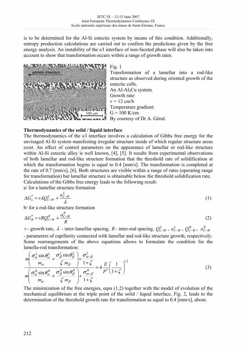
JETC IX – 12-15 June 2007 Joint European Thermodynamics Conference IX
Ecole nationale supérieure des mines de Saint-Étienne, France
212
is to be determined for the Al-Si eutectic system by means of this condition. Additionally, entropy production calculations are carried out to confirm the predictions given by the free energy analysis. An instability of the s/l interface of non-faceted phase will also be taken into account to show that transformation occurs within a range of growth rates.
Fig. 1 Transformation of a lamellar into a rod-like structure as observed during oriented growth of the eutectic cells. An Al-Al2Cu system. Growth rate: v = 12 cm/h Temperature gradient: G = 100 K/cm By courtesy of Dr A. Góral.
Thermodynamics of the solid / liquid interface The thermodynamics of the s/l interface involves a calculation of Gibbs free energy for the envisaged Al-Si system manifesting irregular structure inside of which regular structure areas exist. An effect of control parameters on the appearance of lamellar or rod-like structure within Al-Si eutectic alloy is well known, [4], [5]. It results from experimental observations of both lamellar and rod-like structure formation that the threshold rate of solidification at which the transformation begins is equal to 0.4 [mm/s]. The transformation is completed at the rate of 0.7 [mm/s], [6]. Both structures are visible within a range of rates (operating range for transformation) but lamellar structure is obtainable below the threshold solidification rate. Calculations of the Gibbs free energy leads to the following result: a/ for a lamellar structure formation
λλ
LWCL
WCLaQvG −
− +=Δ * (1)
b/ for a rod-like structure formation
RavRQG
RWCR
WCR−
− +=Δ * (2)
v - growth rate, λ - inter-lamellar spacing, R - inter-rod spacing, LWCQ − , L
WCa − , ,RWCQ − R
WCa − - parameters of capillarity connected with lamellar and rod-like structure growth, respectively. Some rearrangements of the above equations allows to formulate the condition for the lamella-rod transformation:
5.1
* 114
1sinsin
1sinsin
⎟⎟⎠
⎞⎜⎜⎝
⎛+
=
++⎟
⎟⎠
⎞⎜⎜⎝
⎛+
++⎟⎟⎠
⎞⎜⎜⎝
⎛+
−
−
ζζ
σζ
θσθσ
ζσ
ζθσθσ
βα
β
ββ
α
αα
βα
β
ββ
α
αα
PE
mmm
mmm
RRRRR
LLLLL
(3)
The minimization of the free energies, eqns (1,2) together with the model of evolution of the mechanical equilibrium at the triple point of the solid / liquid interface, Fig. 2, leads to the determination of the threshold growth rate for transformation as equal to 0.4 [mm/s], about.
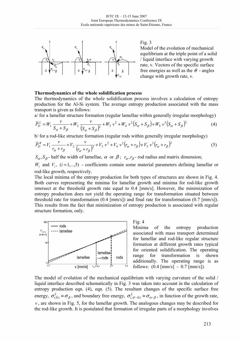
JETC IX – 12-15 June 2007 Joint European Thermodynamics Conference IX
Ecole nationale supérieure des mines de Saint-Étienne, France
213
Fig. 3 Model of the evolution of mechanical equilibrium at the triple point of a solid / liquid interface with varying growth rate, v. Vectors of the specific surface free energies as well as the θ - angles change with growth rate, v.
Thermodynamics of the whole solidification process The thermodynamics of the whole solidification process involves a calculation of entropy production for the Al-Si system. The average entropy production associated with the mass transport is given as follows: a/ for a lamellar structure formation (regular lamellae within generally irregular morphology)
( ) ( ) ( )235
24
23221 βαβα
βαβαSSvWSSvWvW
SSvW
SSvWP L
D ++++++
++
= (4)
b/ for a rod-like structure formation (regular rods within generally irregular morphology)
( ) ( ) ( )235
24
23221 βαβα
βαβαrrvVrrvVvV
rrvV
rrvVP R
D ++++++
++
= (5)
βα SS , - half the width of lamellae, α or β ; βα rr , - rod radius and matrix dimension;
iW and iV , )5,...,1( =i - coefficients contain some material parameters defining lamellar or rod-like growth, respectively. The local minima of the entropy production for both types of structures are shown in Fig. 4. Both curves representing the minima for lamellar growth and minima for rod-like growth intersect at the threshold growth rate equal to 0.4 [mm/s]. However, the minimization of entropy production does not yield the operating range for transformation situated between threshold rate for transformation (0.4 [mm/s]) and final rate for transformation (0.7 [mm/s]). This results from the fact that minimization of entropy production is associated with regular structure formation, only.
Fig. 4 Minima of the entropy production associated with mass transport determined for lamellar and rod-like regular structure formation at different growth rates typical for oriented solidification. The operating range for transformation is shown additionally. The operating range is as follows: (0.4 [mm/s] - 0.7 [mm/s]).
The model of evolution of the mechanical equilibrium with varying curvature of the solid / liquid interface described schematically in Fig. 3 was taken into account in the calculation of entropy production eqn. (4), eqn. (5). The resultant changes of the specific surface free energy, βσσ ≡L
Si)( , and boundary free energy, βασσ −− ≡LSiAl )( , in function of the growth rate,
v , are shown in Fig. 5, for the lamellar growth. The analogous changes may be described for the rod-like growth. It is postulated that formation of irregular parts of a morphology involves
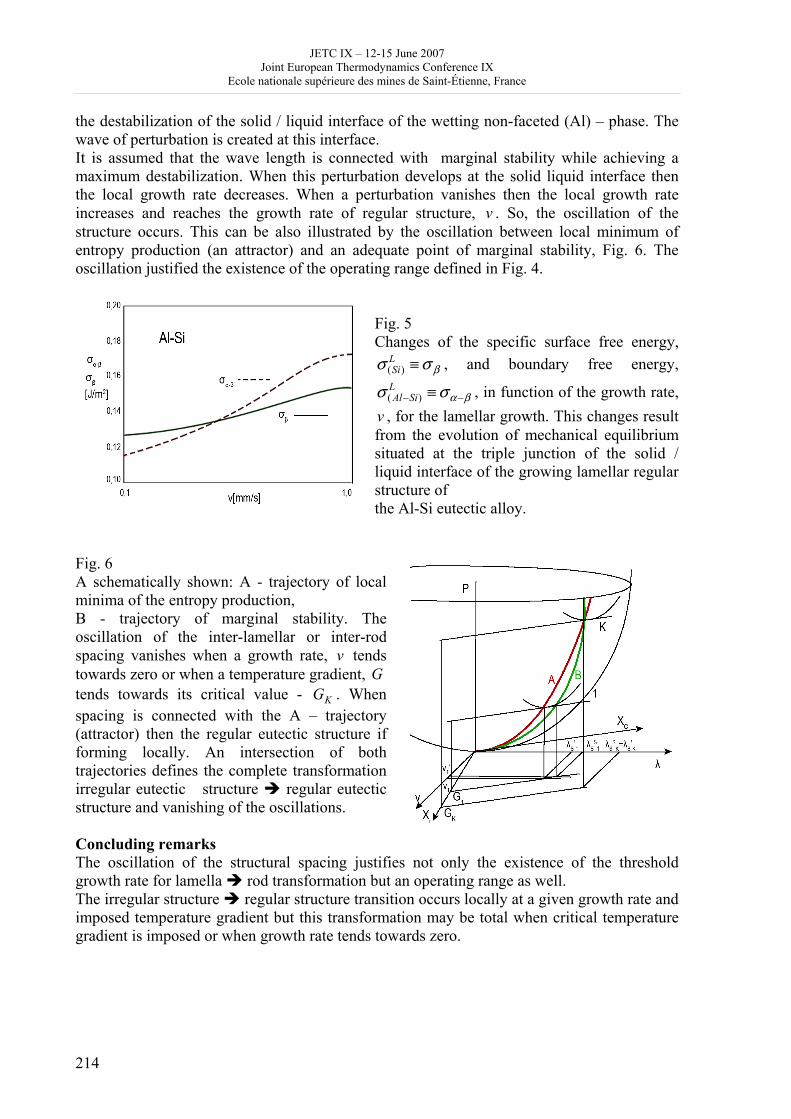
JETC IX – 12-15 June 2007 Joint European Thermodynamics Conference IX
Ecole nationale supérieure des mines de Saint-Étienne, France
214
the destabilization of the solid / liquid interface of the wetting non-faceted (Al) – phase. The wave of perturbation is created at this interface. It is assumed that the wave length is connected with marginal stability while achieving a maximum destabilization. When this perturbation develops at the solid liquid interface then the local growth rate decreases. When a perturbation vanishes then the local growth rate increases and reaches the growth rate of regular structure, v . So, the oscillation of the structure occurs. This can be also illustrated by the oscillation between local minimum of entropy production (an attractor) and an adequate point of marginal stability, Fig. 6. The oscillation justified the existence of the operating range defined in Fig. 4.
Fig. 5 Changes of the specific surface free energy,
βσσ ≡LSi)( , and boundary free energy,
βασσ −− ≡LSiAl )( , in function of the growth rate,
v , for the lamellar growth. This changes result from the evolution of mechanical equilibrium situated at the triple junction of the solid / liquid interface of the growing lamellar regular structure of the Al-Si eutectic alloy.
Fig. 6 A schematically shown: A - trajectory of local minima of the entropy production, B - trajectory of marginal stability. The oscillation of the inter-lamellar or inter-rod spacing vanishes when a growth rate, v tends towards zero or when a temperature gradient, G tends towards its critical value - KG . When spacing is connected with the A – trajectory (attractor) then the regular eutectic structure if forming locally. An intersection of both trajectories defines the complete transformation irregular eutectic structure regular eutectic structure and vanishing of the oscillations. Concluding remarks The oscillation of the structural spacing justifies not only the existence of the threshold growth rate for lamella rod transformation but an operating range as well. The irregular structure regular structure transition occurs locally at a given growth rate and imposed temperature gradient but this transformation may be total when critical temperature gradient is imposed or when growth rate tends towards zero.

JETC IX – 12-15 June 2007 Joint European Thermodynamics Conference IX
Ecole nationale supérieure des mines de Saint-Étienne, France
215
Bibliography [1] J.D.Hunt J.P.Chilton, Journal of the Institute of Metals, 91, (1962/63), 338-342. [2] J.P.Chilton, W.C.Winegard, Journal of the Institute of Metals, 89, (1960/61), 162-168. [3] K.A.Jackson, J.D.Hunt, Transactions of the AIME 236, (1966), 1129-1142. [4] B.Toloui, A.Hellawell, Acta Metallurgica 24, (1976), 565-572. [5] O.A.Atasoy, Aluminium, 60, (1984), 109-116. [6] R.Cupryś, B.Major, W.Wołczyński, Materials Science Forum, 329/330, (2000), 161-166.
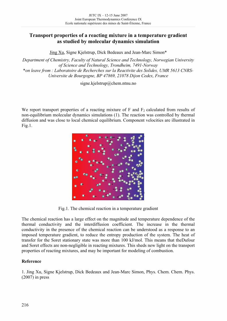
JETC IX – 12-15 June 2007 Joint European Thermodynamics Conference IX
Ecole nationale supérieure des mines de Saint-Étienne, France
216
Transport properties of a reacting mixture in a temperature gradient as studied by molecular dynamics simulation
Jing Xu, Signe Kjelstrup, Dick Bedeaux and Jean-Marc Simon*
Department of Chemistry, Faculty of Natural Science and Technology, Norwegian University of Science and Technology, Trondheim, 7491-Norway
*on leave from : Laboratoire de Recherches sur la Reactivite des Solides, UMR 5613 CNRS-Universite de Bourgogne, BP 47869, 21078 Dijon Cedex, France
We report transport properties of a reacting mixture of F and F2 calculated from results of non-equilibrium molecular dynamics simulations (1). The reaction was controlled by thermal diffusion and was close to local chemical equilibrium. Component velocities are illustrated in Fig.1.
Fig.1. The chemical reaction in a temperature gradient
The chemical reaction has a large effect on the magnitude and temperature dependence of the thermal conductivity and the interdiffusion coefficient. The increase in the thermal conductivity in the presence of the chemical reaction can be understood as a response to an imposed temperature gradient, to reduce the entropy production of the system. The heat of transfer for the Soret stationary state was more than 100 kJ/mol. This means that theDufour and Soret effects are non-negligible in reacting mixtures. This sheds new light on the transport properties of reacting mixtures, and may be important for modeling of combustion.
Reference
1. Jing Xu, Signe Kjelstrup, Dick Bedeaux and Jean-Marc Simon, Phys. Chem. Chem. Phys. (2007) in press
JETC IX – 12-15 June 2007 Joint European Thermodynamics Conference IX
Ecole nationale supérieure des mines de Saint-Étienne, France
217
Convective instabilities of ternary mixtures in thermogravitational columns
Abdelfattah Zebib
Mechanical & Aerospace Engineering Rutgers University, Piscataway, NJ 08854, USA
[email protected] Convective instabilities in side heated infinite vertical slots containing a single fluid are stationary, shear driven when the Prandtl number .≤Pr 12 5 while they are oscillatory, buoyancy dominated with .≥Pr 12 5 due to the diminished influence of the thermal diffusivity with increasing Pr . In [1] we addressed the influence of the Soret effect on this instability in binary mixtures. Here we examine the influence of the concentration field generated by thermodiffusion in a ternary mixture of otherwise uniform concentration on this phenomenon. We first derive expressions and calculate the basic steady one-dimensional flow taking into account the vertical concentration gradients caused by thermodiffusion. Linear stability of this basic state is performed and the critical Rayleigh number, wavenumber and frequency are determined as function of the two separation ratios, ratio of thermal expansivities, four Lewis numbers, and Pr . The results are in excellent agreement with the base flow of the ternary mixture considered in [2,3]. Stability results agree very well with those from a simplified model in the long wave approximation [4]. Stability restrictions on the operation of the thermogravitational column for the ternary mixture [2,3] will be discussed. References [1]A. Zebib, J. Noneq. Therm. (2007), in press [2]A. Leahy-Dios, M. Bou-Ali, J. Platten & A. Firoozabadi J. Chem. Phys. 122 (2005) [3]I. Ryzhkov & V. Shevtsova, Phys. Fluids (2007), in press [4]I. Ryzhkov & V. Shevtsova, (2006), private comm.

JETC IX – 12-15 June 2007 Joint European Thermodynamics Conference IX
Ecole nationale supérieure des mines de Saint-Étienne, France
218
JETC IX – 12-15 June 2007 Joint European Thermodynamics Conference IX
Ecole nationale supérieure des mines de Saint-Étienne, France
219
List and numbers of posters 1 • C. Giraldo et al.: Ethane gaz hydrate incipient conditions in reversed micelles 2 • D. Vasilyev and A. Udovsky: Interconsistency between three types of diagrams for calculation of optimized thermodynamic properties of alloys of the U-Zr system 3 • JF Dalloz: New equations of state for various gases (Ar, CO2, C2 H2 , C2H4, NH3, N2, O2) obtained from experimental data 4 • A. Abbaci and A. Acidi: Supercritical fluids: case of hexane 5 • A. Bougrine et al.: Determination of liquid/vapour equilibria by ebulliometry and modelling by the quasi-ideal model 6 • E. Labarthe et al.: Determination of solid-liquid equilibria in the ternary system piperidine-sodium sulphate water by isoplethic thermic analysis: study of the isothermal sections 293K, 298K, 313K 7 • P. Paricaud et al.: Recent advances in the use of the SAFT approach to describe the phase behaviour of associating molecules, electrolytes and polymers 8 • M. Lakhssassi et al. : A “magmatic isotherm” for the exchange of Fe and M between an olivine solid solution and a melt 9 • A. Udovsky and M Kupavtsev: The development of software for automatic computer program for calculation of two-phase tie-lines and thermodynamic properties of two-phase alloys in closed ternary systems using the natural coordinates 10 • G. Beretta: Non linear generalization of Schrödinger’s equation uniting quantum mechanics and thermodynamics 11 • C. Firat and A Sisman: Quantum surface energy and lateral forces in ideal gases 12 • A Truyol: Thermodynamics and nanosciences and nanotechnologies 13 • F Dennery: Entropy grows whatever the signs of temperature and time in their arrows 14 • P. Galenko and V. Lebedev: Local non-equilibrium effect on spinodal decomposition in a binary system 15 • J. Garrido: Thermodynamics of electrodialysis processes 16 • M. Feidt et al.: What’s new with thermodynamic optimization of refrigerating machines, with regards to design and control-command: a review synthesis
JETC IX – 12-15 June 2007 Joint European Thermodynamics Conference IX
Ecole nationale supérieure des mines de Saint-Étienne, France
220
17 • M. Nikaien et al.: Thermodynamic optimization of Brayton cycle wih steam engine injection using exergy analysis 18 • M. Serier and A Serier: Evolutions thermodynamics of a driving fluid in a cylinder with valves 19 • M. Radulescu et al.: Hybrid combined heat and power plants using a solid oxide fuel cell and external steam reformer 20 • P. Blanco et al.: A predictive phenomenological law of the thermodiffusion coefficient in organic mixtures of n-alkanes nCi- nCj (i, j = 5, …, 18) at 25 ° and 50 wt% 21 • W. Kölher et al.: A systematic study of the Soret coefficient of binary liquid mixtures 22 • A. Zebib: Convective instabilities of ternary mixtures in thermogravitational columns 23 • P. Polyakov: Study of thermal diffusion behaviour of alkane/benzene mixtures by thermal diffusion forced Rayleigh scattering experiments and lattice model calculations 24 • A. Mialdun: Measurement of Soret coefficients in aqueous solutions 25 • B Guy: Geology and thermodynamics
JETC IX – 12-15 June 2007 Joint European Thermodynamics Conference IX
Ecole nationale supérieure des mines de Saint-Étienne, France
221
Geological field trip, 15 June 2007 Departure: Saint-Etienne: 8h 30 9h 30 : First stop: Col du Pertuis View point (Le Puy area, Devès etc.) : the different types of volcanic rocks as seen in the landscape (different geomorphologic behavior): basaltic cones and flows, trachyte and phonolithe intrusions… The problem to understand the link between these different rocks in the same area. 10h 30: Second stop: suc de Monac The phonolithic dyke of Monac: inspection of the rock. General view of the outcrop. 11h 30: Third stop: basaltic lava lake of Noustoulet The basaltic rock and its peridotites enclaves. The columnar jointing of basalts. General discussion: - fractionate cristallization of magmas and phase diagrams - partial fusion of peridotites and the formation of basalts - geothermometers and geobarometers and the physical conditions for the formation of enclaves - columnar jointing of basalts: constitution undercooling or thermal induced stress? 13h: Saint-Jullien Chapteuil Lunch 15h : End 16h: Back to Saint-Etienne

JETC IX – 12-15 June 2007 Joint European Thermodynamics Conference IX
Ecole nationale supérieure des mines de Saint-Étienne, France
222
JETC IX – 12-15 June 2007 Joint European Thermodynamics Conference IX
Ecole nationale supérieure des mines de Saint-Étienne, France
223
Exhibition on thermodynamics
An exhibition on thermodynamics will be prepared by the students of Ecole des mines under the supervision of La ROTONDE group (Popularisation of Science) led by Emilie POURCHEZ: history of thermodynamics, important names, great inventions etc. Making of models. Special activities: history of steam machine and steam locomotive for which engineers from Saint-Etienne brought important improvement in the XIXth century. The exhibition will be visited by young schoolboys and schoolgirls from Saint-Etienne area. The way they react to the exhibition will be studied by a group of researchers from Ecole normale supérieure de Lyon (pedagogy of science).
Message of the students (Fabien Le Bars, Bruno Renié, Benoît Richard, Pierre Sallot, Monard Vong):
“Today, science is more and more present in our life through the different issues of global warming, renewable sources of energy, scientific research on cancer. So, that is why popularisation of science is of the essence. As far as we are concerned, we, the students of Ecole nationale supérieure des mines de Saint-Etienne, have just tried to offer young scholars some keys to better understand thermodynamics and to follow a kind of scientific approach of these phenomena. To conclude with, we hope this workshop will stir up their curiosity thanks to amazing experiments. We have set up three devices to show the usage of thermodynamics we make in everyday life.
The first one consists in designing a little boat propelled by an engine only made up with a metal tube and a little candle.
An other device will show a reduced model of a Stirling engine. We will try to explain how a temperature difference can be converted to physical movement.
The last device is an "entertaining chemistry" experiment : we will set up an oscillating chemical reaction which we will explain simply. Our goal is here to show that chemistry can be sympathetic and easy to understand.”

JETC IX – 12-15 June 2007 Joint European Thermodynamics Conference IX
Ecole nationale supérieure des mines de Saint-Étienne, France
224
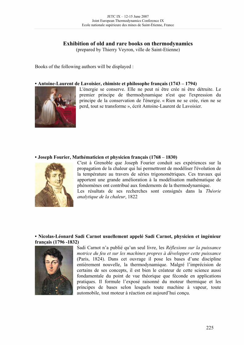
JETC IX – 12-15 June 2007 Joint European Thermodynamics Conference IX
Ecole nationale supérieure des mines de Saint-Étienne, France
225
Exhibition of old and rare books on thermodynamics
(prepared by Thierry Veyron, ville de Saint-Etienne) Books of the following authors will be displayed : • Antoine-Laurent de Lavoisier, chimiste et philosophe français (1743 – 1794)
L'énergie se conserve. Elle ne peut ni être crée ni être détruite. Le premier principe de thermodynamique n'est que l'expression du principe de la conservation de l'énergie. « Rien ne se crée, rien ne se perd, tout se transforme », écrit Antoine-Laurent de Lavoisier.
• Joseph Fourier, Mathématicien et physicien français (1768 – 1830)
C'est à Grenoble que Joseph Fourier conduit ses expériences sur la propagation de la chaleur qui lui permettront de modéliser l'évolution de la température au travers de séries trigonométriques. Ces travaux qui apportent une grande amélioration à la modélisation mathématique de phénomènes ont contribué aux fondements de la thermodynamique. Les résultats de ses recherches sont consignés dans la Théorie analytique de la chaleur, 1822
• Nicolas-Léonard Sadi Carnot usuellement appelé Sadi Carnot, physicien et ingénieur français (1796 -1832)
Sadi Carnot n’a publié qu’un seul livre, les Réflexions sur la puissance motrice du feu et sur les machines propres à développer cette puissance (Paris, 1824). Dans cet ouvrage il pose les bases d’une discipline entièrement nouvelle, la thermodynamique. Malgré l’imprécision de certains de ses concepts, il est bien le créateur de cette science aussi fondamentale du point de vue théorique que féconde en applications pratiques. Il formule l’exposé raisonné du moteur thermique et les principes de bases selon lesquels toute machine à vapeur, toute automobile, tout moteur à réaction est aujourd’hui conçu.
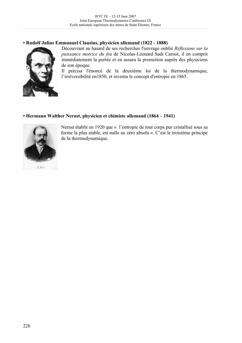
JETC IX – 12-15 June 2007 Joint European Thermodynamics Conference IX
Ecole nationale supérieure des mines de Saint-Étienne, France
226
• Rudolf Julius Emmanuel Clausius, physicien allemand (1822 - 1888)
Découvrant au hasard de ses recherches l'ouvrage oublié Réflexions sur la puissance motrice du feu de Nicolas-Léonard Sadi Carnot, il en comprit immédiatement la portée et en assura la promotion auprès des physiciens de son époque. Il précisa l'énoncé de la deuxième loi de la thermodynamique, l’irréversibilité en1850, et inventa le concept d'entropie en 1865.
• Hermann Walther Nernst, physicien et chimiste allemand (1864 – 1941)
Nernst établit en 1920 que « l’entropie de tout corps pur cristallisé sous sa forme la plus stable, est nulle au zéro absolu ». C’est le troisième principe de la thermodynamique.
JETC IX – 12-15 June 2007 Joint European Thermodynamics Conference IX
Ecole nationale supérieure des mines de Saint-Étienne, France
227
Ceilidh
Social folk dance (Ceilidh) – Thursday evening 14 June 2007 After the Colloquium has finished on Thursday evening, 14th June members of JETCIX are invited to a social folk dance (Ceilidh) with a local club called “Danses sans Frontières” (DSF) at Villars, a small suburb on the northern outskirts of St Etienne. There will be live Scottish music provided by Pascal Rosiak (chromatic accordion), and French music played by two local musicians from Doizieux Yakafolké (Martine and Jean-Philippe) on diatonic button accordions. The JETCIX dance will officially begin at 22h00 and continue until midnight at “La salle de la Libération” Villars. You are welcome at Danses sans Frontières after 21h00 when you can freely participate with members of DSF who will be practicing various dances from Israel. Some members of DSF will stay after 22h00 to assist with the fok dance (Ceilidh) for example if you need help with the dance or you are looking for a dancing partner. It is important to indicate on registration that you wish to participate at the folk dance and to reserve a place on the coach for yourself, and any other accompanying person. There will be a small charge of 5€ per person. The coach will leave Saint Etienne at 21h00 precisely returning at 00h30. Peter Bowden Ceilidh co-ordinator
JETC IX – 12-15 June 2007 Joint European Thermodynamics Conference IX
Ecole nationale supérieure des mines de Saint-Étienne, France
228
What is ECAST ? European Center for Advanced Studies in Thermodynamics Statutes: Association according to French law, governed by the law of the 1st July 1901 and the decree of August 16, 1901. Goal: Promote the cooperation between researchers and engineers in Europe to develop scientific and technical interactions in the domain of thermodynamics and energetics. Composition: group of physical persons or legal entities in Europe interested by the study, the research, the teaching, the information, the normalization, the legislation, the application and the use of thermodynamics. Activities: Organization of scientific and technical meetings in the aforementioned domains. Disseminating information relating to the schedule of international conferences and to the recent papers in the implied sciences. Investigating about the offers and the requests for studies by thermodynamicists likely to promote the new discoveries of their specialties. Developing the relations with other European associations interested by thermodynamics and energetics. Encouragement of European cooperation in the teaching, the research in laboratories and the use, by appropriate gathering of complementary means regarding theory, experiment and computation. Consultations with the national or European organisms on the possibilities to insert the preceding activities in the programs of actions proposed by these administrations. (the complete statutes of the association will be communicated to every person on request)
JETC IX – 12-15 June 2007 Joint European Thermodynamics Conference IX
Ecole nationale supérieure des mines de Saint-Étienne, France
229
List of authors by alphabetic order of the first authors
A. Abbaci and A. Acidi........................................................................................................................................ 16 Faculté des Sciences, Département de Chimie, Université Badji-Mokhtar B. P. 12, El-Hadjar, Annaba (23200) [email protected]
Bjarne Andresen1 and Christopher Essex2........................................................................................................ 17 1 Niels Bohr Institute, University of Copenhagen, Universitetsparken 5, DK-2100 Copenhagen Ø, Denmark 2 Department of Applied Mathematics, University of Western Ontario, London ON, N6A 5B7, Canada [email protected], [email protected]
Magdalena Bendová, a Zdeněk Wagner, a Michal Moučka b........................................................................... 19 a Institute of Chemical Process Fundamentals, Academy of Sciences of the Czech Republic, Rozvojová 135, 165 02 Prague 6, Czech Republic b Department of Applied Cybernetics, Technical University of Liberec, Hálkova 6, 461 17 Liberec. Czech Republic [email protected] - [email protected]
Gian Paolo Beretta .............................................................................................................................................. 24 Università di Brescia, Italy [email protected]
Gian Paolo Beretta .............................................................................................................................................. 30 Università di Brescia, Italy [email protected] - www.quantumthermodynamics.org
P. Blanco1, M.M Bou-Ali1, J.K. Platten2, J.A. Madariaga3, P. Urteaga1 and C Santamaría3 ...................... 36 1Manufacturing Department, MGEP Mondragon Goi Eskola Politeknikoa Loramendi 4, Apartado 23, 20500 Mondragon, Spain. 2University of Mons-Hainaut, avenue du Champs de Mars 24, B-7000 Mons, Belgium 3Departamento de Fisica Aplicada II, Universidad del Pais Vasco, Apdo 644, 48080 Bilbao, Spain [email protected]
A.J. Bougrine, E. Labarthe, C. Blanchard, O. Duclos, R. Tenu, H. Delalu, C. Goutaudier ......................... 40 Laboratoire Hydrazines et Procédés, UMR 5179 Université Claude Bernard Lyon 1 – CNRS – Isochem/SNPE 43, Bd du 11 Novembre 1918, 69622 Villeurbanne Cedex, France [email protected]
Danièle Clausse1, Isabelle Pezron 1, Moncef Stambouli2 and Jean- Louis Grossiord3................................... 42 1 Université de Technologie de Compiègne. Département de Génie Chimique. BP 20529 60205 Compiègne France 2 Ecole Centrale Paris- Laboratoire de Génie des Procédés et Matériaux- 92 296 Chatenay-Malabry 3 Université de Paris Sud, Laboratoire de Physique Pharmaceutique, UMR CNRS 8612, 92296 Châtenay-Malabry, France. [email protected]
F. Couenne , C. Jallut, B. Maschke .................................................................................................................... 43 Université de Lyon, Université Lyon 1, Laboratoire d’Automatique et de Génie des Procédés, UMR CNRS 5007, ESCPE, 43 Bd du 11 Novembre 1918, 69622 Villeurbanne cedex [email protected]
Jean-François Dalloz........................................................................................................................................... 47 La Seyne, 83 500, France [email protected]
François-Xavier Demoures ................................................................................................................................. 48 Ecole Normale Supérieure Lettres et Sciences Humaines (Lyon) department of Philosophy [email protected]
JETC IX – 12-15 June 2007 Joint European Thermodynamics Conference IX
Ecole nationale supérieure des mines de Saint-Étienne, France
230
F.M. Dennery .......................................................................................................................................................49 Hon. prof. E.C.P francis.dennery @ wanadoo.fr
Prof.em.dr.ir. J. de Swaan Arons .......................................................................................................................53 Delft University of Technology Delft, The Netherlands and Royal Dutch Shell Chair Chemical Engineering Dept. Tsinghua University Beijing, China [email protected]
Alexis De Vos and Yvan Van Rentergem ..........................................................................................................54 Imec v.z.w. and Universiteit Gent Sint-Pietersnieuwstraat 41, B-9000 Gent, Belgium [email protected]
Jordi Faraudo1,2, Fernando Bresme3..................................................................................................................58 1 Dept. de Física, Universitat Autònoma de Barcelona , E-08193 Bellaterra, Spain 2Institut de Ciència de Materials de Barcelona (ICMAB-CSIC), Campus UAB, E-08193 Bellaterra, Spain 3 Department of Chemistry, Imperial College, London SW7 2AZ, UK [email protected]
M. Feidt 1, M. Karkri 1, R. Boussehain 1, M. Costea2, C. Petre2, S. Petrescu2 ................................................62 1 LEMTA-UHP, NANCY, France 2 Faculté de Génie Mécanique, UPB BUCAREST, Roumanie [email protected]
Coskun Firat and Altug Sisman*........................................................................................................................68 Istanbul Technical University, Energy Institute, 34469 Maslak, Istanbul, Turkey. [email protected], [email protected]
Peter Galenko(1) and David Jou(2) .......................................................................................................................75 (1)German Aerospace Center, Institute of Materials Physics in Space, 51170 Cologne, Germany (2)Departament de Fisica, Universitat Autonoma de Barcelona, 08193 Bellaterra, Catalonia, Spain [email protected] - [email protected]
Peter Galenko(1) and Vladimir Lebedev(2)..........................................................................................................80 (1)German Aerospace Center, Institute of Materials Physics in Space, 51170 Cologne, Germany e-mail: (2)Udmurt State University, Department of Theoretical Physics, 426034 Izhevsk, Russia [email protected] - [email protected]
Javier Garrido......................................................................................................................................................82 Departamento de Física de la Tierra y Termodinámica, Universitat de València, E-46100 Burjassot (Valencia), Spain [email protected]
Carlos Giraldo1 , Daniel Ehlers2, Lothar Oellrich2, Matthew Clarke1 ............................................................84 1 Department of Chemical & Petroleum Engineering University of Calgary 2500 University Drive Calgary, Alberta, Canada, T2N 1N4 2 Institut für Technische Thermodynamik und Kältetechnik Universität Karlsruhe Engler-Bunte-Ring 21 Karlsruhe, Germany, 76131 [email protected]
Fabien Girarda, Mickaël Antonia, Sylvain Faureb and Annie Steinchen-Sanfelda .........................................89 a Laboratoire de Thermodynamique et de Modélisation des Milieux hors Equilibre, UMR-CNRS 6171, Université Paul Cézanne Aix-Marseille BP 451, F-13397, Marseille cedex 20 (France) b CEA-Marcoule, Laboratoire des Procédés Avancés de Décontamination, DTCD/SPDE/LPAD, Bât. 222, F-30207 Bagnols/Cèze Cedex (France)
Bernard GUY.......................................................................................................................................................90 Ecole nationale supérieure des mines de Saint-Etienne, France [email protected]
JETC IX – 12-15 June 2007 Joint European Thermodynamics Conference IX
Ecole nationale supérieure des mines de Saint-Étienne, France
231
Bernard GUY....................................................................................................................................................... 92 Ecole nationale supérieure des mines de Saint-Etienne, France [email protected]
S.L Hafsaoui, M. Ould Slimane and R. Mahmoud........................................................................................... 94 Ecole Militaire Polytechnique, BP17, Bordj El Bahri, 16111, Algeria [email protected]
Karl Heinz Hoffmann1 ........................................................................................................................................ 95 1 Institut für Physik – Technische Universität Chemnitz – 09107 Chemnitz – Germany [email protected]
W. Köhler, G. Wittko, S. Hartmann................................................................................................................ 100 Physikalisches Institut, Universität Bayreuth, Germany [email protected]
E. LABARTHE, N. KACIDEM, A.J. BOUGRINE,C. GOUTAUDIER, J.J COUNIOUX, H. DELALU . 104 Laboratoire Hydrazines et Procédés-Université Claude Bernard Lyon 1-69622 VILLEURBANNE [email protected]
Morad Lakhssassi, Jacques Moutte and Bernard Guy .................................................................................. 106 Ecole nationale supérieure des mines de Saint-Etienne, France [email protected]
Ahmed Laouir1, Daniel Tondeur2 .................................................................................................................... 108 1 University of Jijel, Faculty of Engineering Ouled Aissa BP 98- 18000 Jijel Algeria. [email protected] 2
Laboratoire des Sciences du Génie Chimique, INPL-LSGC 1, rue Grandville BP 451- 54001 Nancy France. [email protected]
Le Marechal Jean-François, El Bilani Rania .................................................................................................. 113 UMR I.C.A.R., INRP, CNRS, Université de Lyon, France [email protected], [email protected]
Stefano Mazzoni, F. Giavazzi, R. Cerbino, M. Giglio and A. Vailati............................................................ 114 European Space Agency - ESTEC HME-GAP, Keplerlaan 1, 2201AZ, Noordwijk ZH, The Netherlands [email protected]
Vicenç Méndez and José Casas-Vázquez ........................................................................................................ 116 Grup de Física Estadística. Departament de Física. Universitat Autònoma de Barcelona. E-08193 Bellaterra (Cerdanyola) Spain. [email protected], [email protected]
Alexandr Mialdun, Valentina Shevrsova ........................................................................................................ 121 MRC, Department of Chemical Physics, Université Libre de Bruxelles CP 165/62, av. F.D. Roosevelt 50, B–1050 Brussels, Belgium [email protected]
Jacques Moutte .................................................................................................................................................. 125 Géochimie, Ecole des Mines de Saint Etienne, France [email protected]
M.Nikaien1, H.Ajam2, S.M.Hoseini Sarvari2 ................................................................................................... 127 S.B University, Department of Mechanical Engineering, University St., Zahedan, Iran [email protected]
JETC IX – 12-15 June 2007 Joint European Thermodynamics Conference IX
Ecole nationale supérieure des mines de Saint-Étienne, France
232
Bernd R. Noack1, Michael Schlegel1, oye Ahlborn2, Gerd Mutschke3, Marek Morzynki4, Pierre Comte5
and Gilead Tadmor6 ..........................................................................................................................................129 1 Berlin University of Technology, D-10623 Berlin, Germany 2 University of British Columbia, Vancouver V6Z 1Z1, Canada 3 Forschungszentrum Dresden-Rossendorf, Postfach 510119, D-01314 Dresden, Germany 4
Poznań University of Technology, PL-60-965 Poznań, Poland 5 Université de Poitiers, F-86036 Poitiers Cedex, France 6 Northeastern University, Boston, MA 02115, USA [email protected]
E. Nourtier-Mazauric1, B. Guy2, D. Garcia2....................................................................................................133 1 Laboratoire Jean Kuntzmann, Grenoble, France 2 Ecole nationale supérieure des mines de Saint-Etienne, France [email protected], [email protected], [email protected]
Patrice Paricaud1*, Walter Furst 1, Christophe Coquelet2, Amparo Galindo3, George Jackson3. .............135 1 Laboratoire de Chimie et Procédés, ENSTA, Paris, France; 2 Laboratoire de Thermodynamique des Equilibres de Phase, Ecole des Mines de Paris, Fontainebleau. 3 Chemical Engineering Department, Imperial College, London, UK. [email protected]
Patrice Paricaud1*, Jose L. Rivera2, Milan Předota3, Ariel A. Chialvo4, Peter T. Cummings4,5 ................136 1 Laboratoire de Chimie et Procédés, ENSTA, Paris, France; 2 Department of Physics, Wesleyan University, Middletown, CT, 06459, USA. 3 Department of Medical Physics and Biophysics, University of South Bohemia, Jírovcova 24, České Budějovice, 370 04, Czech Republic. 4 Chemical Sciences Division, Aqueous Chemistry and Geochemistry Group, Oak Ridge National Laboratory, Oak Ridge, Tennessee 37831-6110. 5 Department of Chemical Engineering, Vanderbilt University, Nashville, TN 37235-1604, USA. [email protected]
Erwan PERFETTI1, Jean DUBESSY1, Régis THIERY2................................................................................137 1 : G2R (UMR 7566), Faculté des Sciences, UHP, BP-239-54506-Vandoeuvre-lès Nancy, Cedex, France : [email protected]: [email protected] 2 : UMR LMV 6524, Université Blaise Pascal, 5 rue Kessler, F-63038 Clermont-Ferrand Cedex [email protected]
Pierre Perrot ......................................................................................................................................................141 Laboratoire de Métallurgie Physique, Université des Sciences et technologies de Lille [email protected]
Pavel Polyakov1, Jutta Luettmer-Strathmann2 and Simone Wiegand1........................................................146 1 Forschungszentrum Juelich GmbH, IFF - Weiche Materie, D-52428 Juelich, Germany 2 Department of Physics and Department of Chemistry, The University of Akron, Akron, Ohio 44325-4001 [email protected]
Michel PONS......................................................................................................................................................150 CNRS-LIMSI, BP 133, 91403 Orsay Cedex, France michel.pons @ limsi.fr
Jean-François Portha1, Jean-Noël Jaubert2, Marie-Noëlle Pons1, Thorsten Burkhardt3, Frédéric Hoffmann3...........................................................................................................................................155
1 Laboratoire des Sciences du Génie Chimique, CNRS-ENSIC-INPL, Nancy 2 Laboratoire de Thermodynamique des Milieux Polyphasés, ENSIC-INPL, Nancy 3 Institut Français du Pétrole, IFP Lyon [email protected]
Diogo Queiros-Conde1 and Michel Feidt2 .......................................................................................................159 1ENSTA, Unité Chimie et Procédés, 32 Bb Victor, 75015 Paris 2LEMTA, ENSEM-INPL, 2 Av. de la Forêt de Haye, F-54504 Vandoeuvre lès Nancy [email protected]
JETC IX – 12-15 June 2007 Joint European Thermodynamics Conference IX
Ecole nationale supérieure des mines de Saint-Étienne, France
233
Mihai Radulescu1, Olivier Lottin2, Michel Feidt2 ........................................................................................... 163 1 EDF R&D EnerBat, Centre des Renardières, Ecuelles, 77818 Moret sur Loing, France 2 LEMTA, Nancy-University, CNRS, 2 av. Forêt de Haye, BP 160, 54500 Vandoeuvre lès Nancy, France [email protected] [email protected]
Pascal Richet ...................................................................................................................................................... 169 Physique des Minéraux et des Magmas, Institut de Physique du Globe, 4 place Jussieu, 75005 Paris, France [email protected]
Ilya I. Ryzhkov1,2 and Valentina M. Shevtsova1.............................................................................................. 170 1MRC, Department of Chemical Physics, Universite Libre de Bruxelles CP 165/62, av. F.D. Roosevelt 50, B–1050 Brussels, Belgium 2Institute of Computational Modelling SB RAS, 660036 Krasnoyarsk, Russia [email protected]
Sabine Sarraute, Vladimir Majer, Margarida F. Costa Gomes .................................................................... 171 Laboratoire de Thermodynamique des Solutions et des Polymères, Université Blaise Pascal Clermont-Ferrand/CNRS, 63177 Aubière, France [email protected]
Boris Sedunov .................................................................................................................................................... 176 Russian New University, Moscow [email protected]
M.Serier, A.Serier ............................................................................................................................................. 181 Laboratory of covers, materials and environment M' Hamed Bougara university, 35000 Boumerdes - Algeria [email protected]
Stanislaw Sieniutycz .......................................................................................................................................... 185 Faculty of Chemical and Process Engineering Warsaw University of Technology PL 00-645, 1 Waryńskiego Street, Warsaw, Poland
M.Sorina , F. Rheaulta and B. Spinnerb ........................................................................................................... 186 a CANMET Energy Technology Centre -Varennes, 1615 Lionel-Boulet, P.O. Box 4800, Varennes, Quebec,
J3X 1S6, Canada, Tel: (450) 652-3513, Fax: (450) 652-0999, b CNRS-IMP, Institut de Science et Génie des Matériaux et Procédés, UPR 8521, Université, 66860 Perpignan Cedex, France, Tel: 4-68662110, Fax:4-68556869 [email protected]
D. Tondeur ......................................................................................................................................................... 187 Laboratoire des Sciences du Génie Chimique CNRS ENSIC 1 rue Grandville, Nancy
Albert Truyol ..................................................................................................................................................... 188 CERET [email protected]
A.L.Udovsky ...................................................................................................................................................... 189 Baikov Institute of Metallurgy and Materials Science of Russian Academy of Sciences [email protected]
A.L.Udovsky1, M.V.Kupavtsev1 ....................................................................................................................... 194 1 Baikov Institute of Metallurgy and Materials Science of RAS [email protected]
D.A.Vasilyev, A.L.Udovsky .............................................................................................................................. 199 Baikov Institute of Metallurgy and Materials Science RAS, Moscow, Russia [email protected]; [email protected]
JETC IX – 12-15 June 2007 Joint European Thermodynamics Conference IX
Ecole nationale supérieure des mines de Saint-Étienne, France
234
Thierry Veyron ..................................................................................................................................................204 Ville de Saint-Etienne, 42000, France [email protected]
Simone Wiegand, Hui Ning, Johan Buitenhuis, Jan K.G. Dhont ..................................................................206 IFF-Soft condensed mater, Research Center Jülich, Leo-Brandt Str., 52428 Jülich [email protected]
Waldemar WOŁCZYŃSKI ..............................................................................................................................211 Institute of Metallurgy and Materials Science – 25, Reymonta Street, 30059 Kraków, Poland [email protected]
Jing Xu, Signe Kjelstrup, Dick Bedeaux and Jean-Marc Simon* .................................................................216 Department of Chemistry, Faculty of Natural Science and Technology, Norwegian University of Science and Technology, Trondheim, 7491-Norway *on leave from : Laboratoire de Recherches sur la Reactivite des Solides, UMR 5613 CNRS-Universite de Bourgogne, BP 47869, 21078 Dijon Cedex, France [email protected]
Abdelfattah Zebib..............................................................................................................................................217 Mechanical & Aerospace Engineering Rutgers University, Piscataway, NJ 08854, USA [email protected]


Ecole nationale supérieure des mines de Saint-Etienne 158, cours Fauriel – 42023 Saint-Etienne Cedex 2
Place of conference:
29, rue Pontchardier – 42023 Saint-Etienne Cedex 2
Phone : +33 (0)4 77 42 01 23 www.emse.fr/JETCIX