Introduction to

CATEGORY THEORY

and

CATEGORICAL LOGIC

Thomas Streicher

SS 03 and WS 03/04

Contents

1 Categories 5

2 Functors and Natural Transformations 9

3 Subcategories, Full and Faithful Functors, Equivalences 14

4 Comma Categories and Slice Categories 16

5 Yoneda Lemma 17

6 Grothendieck universes : big vs. small 20

7 Limits and Colimits 22

8 Adjoint Functors 36

9 Adjoint Functor Theorems 46

10 Monads 52

11 Cartesian Closed Categories and λ–Calculus 6311.1 Exponentials in Presheaf Categories . . . . . . . . . . . . . . . 6411.2 Categorical semantics of typed λ-calculus in ccc’s . . . . . . . 68

12 Elementary Toposes 77

13 Logic of Toposes 86

14 Some Exercises in Presheaf Toposes 106

15 Sheaves 111

1

Introduction

The aim of this course is to give an introduction to the basic notions ofCategory Theory and Categorical Logic.The first part on Category Theory should be of interest to a general math-ematical audience with interest in algebra, geometry and topology where atleast the language of category theory and some of its basic notions like lim-its, colimits and adjoint functors are indispensible nowadays. However, forfollowing the lectures in a profitable way one should have already attended acourse in basic algebra or topology because algebraic structures like groups,rings, modules etc. and topological spaces serve as the most important sourceof examples illustrating the abstract notions introduced in the course of thelectures.The second part will be of interest to people who want to know about logicand how it can be modelled in categories. In particular, we will presentcartesian closed categories where one can interpret typed λ-calculus, thebasis of modern functional programming languages, and (elementary) toposesproviding a most concise and simple notion of model for constructive higherorder logic. Guiding examples for both notions will be presented en detail.Some knowledge about constructive logic would be helpful (as a motivatingbackground) but is not necessary for following the presentation itself.

We conclude this most concise introduction with a list of suggestions forfurther reading.

References

[ARV] J. Adamek, J. Rosicky, E. Vitale Algebraic Theories. CUP (2011).

[Aw] S. Awodey Category Theory OUP (2006).

[BW1] M.Barr, Ch. Wells Toposes, Triples and Theories Springer (1985).

[BW2] M.Barr, Ch. Wells Category Theory for Computing Science PrenticeHall (1990).

[Bor] F. Borceux Handbook of Categorical Algebra 3 vols., CambridgeUniversity Press (1994).

2

[FS] P.J. Freyd, A. Scedrov Categories, Allegories North Holland (1990).

[Jac] B. Jacobs Categorical Logic and Type Theory North Holland (1999).

[Joh] P. T. Johnstone Sketches of an Elephant. A Topos Theory Com-pendium. 2 vols. OUP (2002).

[JM] A. Joyal, I. Moerdijk Algebraic Set Theory CUP (1995).

[LaS] J. Lambek, P. J. Scott Introduction to Higher Order Categorical LogicCUP (1986).

[LS] F.W. Lawvere, S. Schanuel Conceptual Mathematics CUP (1997).

[LR] F.W. Lawvere, R. Rosebrugh Sets for Mathematics. A first introduc-tion to categories. CUP (2003).

[McL] C. McLarty Elementary Categories, Elementary Toposes OUP(1995).

[ML] S. MacLane Categories for the Working Mathematician Spinger(1971).

[MM] S. MacLane, I. Moerdijk Sheaves in Geometry and Logic. A FirstIntroduction to Topos Theory. Spinger (1992).

[PRZ] M. La Palme Reyes, G. Reyes, H. Zolfaghari Generic figures and theirglueings. A constructive approach to functor categories. Polimetrica(2004).

[PT] P. Taylor Practical Foundations CUP (1999).

3

Part I CATEGORY THEORY

4

1 Categories

We first introduce our basic notion of structure, namely categories.

Definition 1.1 A category C is given by the following data

• a class Ob(C) of objects of C

• a family Mor(C) associating with every pair A,B ∈ Ob(C) a classMor(C)(A,B) of morphisms from A to B

• for all A,B,C ∈ Ob(C) a mapping

A,B,C : Mor(C)(B,C)×Mor(C)(A,B)→ Mor(C)(A,C)

called composition

• for all A ∈ Ob(C) a distinguished morphism

idA ∈ Mor(C)(A,A)

called identity morphism for A

required to satisfy the following conditions

• for all A,B,C,D ∈ Ob(C) and f ∈ Mor(C)(A,B), g ∈ Mor(C)(B,C)and h ∈ Mor(C)(C,D) it holds that

(Ass) h (g f) = (h g) f

standing as an abbreviation for the more explicit, but also more unread-able equation A,C,D(h, A,B,C(g, f)) = A,B,D(B,C,D(h, g), f)

• for all A,B,C ∈ Ob(C) and f ∈ Mor(C)(A,B) and g ∈ Mor(C)(C,A)it holds that

(Id) f idA = f and idA g = g

standing as an abbreviation for the more explicit, but also more unread-able equations A,A,B(f, idA) = f and C,A,A(idA, g) = g. ♦

5

Notice that the identity morphisms are uniquely determined by and therequirement (Id). (Exercise!)

Some remarks on notation.As already in Definition 1.1 we write simply g f instead of the more explicitA,B,C(g, f) whenever f ∈ Mor(C)(A,B) and g ∈ Mor(C)(B,C). Instead ofthe somewhat clumsy Mor(C)(A,B) we often write simply C(A,B) and forf ∈ Mor(C)(A,B) we simply write f : A → B when C is clear from thecontext. Instead of idA we often write 1A or simply A. When the object Ais clear from the context we often write simply id or 1 instead of idA or 1A,respectively.

Next we consider some

Examples of Categories

(1) The category whose objects are sets, whose morphisms from A to Bare the set-theoretic functions from A to B and where composition isgiven by (g f)(x) = g(f(x)) is denoted as Set. Of course, in Set theidentity morphism idA sends every x ∈ A to itself. For obvious reasonswe call Set the category of sets (and functions).

(2) We write Set∗ for the category of sets with a distinguished element(denoted by ∗) and functions preserving this distinguished point.

(3) We write Mon for the category of monoids and monoid homomor-phisms. This makes sense as monoid homomorphisms are closed undercomposition and identity maps preserve the monoid structure.

(4) We write Grp for the full subcategory1 of Mon whose objects aregroups.

(5) We write Ab for the full subcategory of Grp whose objects are theabelian (i.e. commutative) groups.

(6) We write Rng for the category whose objects are rings and whosemorphisms are ring homomorphisms and CRng for the full subcategoryof Rng on commutative rings.

1B is a subcategory of A if Ob(B) ⊆ Ob(A), B(X,Y ) ⊆ A(X,Y ) for all X,Y ∈ Ob(B)and composition and identities in B are inherited from A (by restriction). A subcategoryB of A is called full if B(X,Y ) = A(X,Y ) for all X,Y ∈ Ob(B).

6

(7) For a commutative ring R we write ModR for the category of R-modules and their homomorphisms (if R is a field k then we writeVectk instead of Modk). The category of R-algebras and their homo-morphisms is denoted as AlgR.

(8) We write Sp for the category of topological spaces and continuousmaps.

(9) Identifying homotopy equivalent maps in Sp gives rise to the categorySph.

2

(10) Every monoid M = (M, ·, 1) can be understood as a category with oneobject (usually denoted as ∗). Categories with one object are preciselythe monoids.

(11) Every preorder P = (P,≤) (i.e. where ≤ is a reflexive and transitivebinary relation on P ) can be considered as a category whose objectsare the elements of P and whose morphisms from x to y are given bythe set ∗ | x ≤ y. Categories arising this way are those categories Cwhere C(X, Y ) contains at most one element for all X, Y ∈ Ob(C) andthey are called posetal. ♦

When “inverting the direction of arrows” in a given category this gives riseto the so-called “dual” or “opposite” category Cop which in general is quitedifferent from C.

Definition 1.2 Let C be a category. Then its dual or opposite categoryCop is given by Ob(Cop) = Ob(C), Cop(A,B) = C(B,A) and Cop

A,B,C(g, f) =CC,B,A(f, g). ♦

Obviously, for every object A the morphism idA is the identity morphism forA also in Cop.

Next we consider some properties of morphisms generalising the notions in-jective, surjective and bijective known from Set to arbitrary categories.

2Continuous maps f0, f1 : X → Y are called homotopy equivalent (notation f0 ∼ f1)iff there is a continuous map f : [0, 1] × X → Y with fi(x) = f(i, x) for all x ∈ X andi ∈ 0, 1. One easily checks that f0 ∼ f1 and g0 ∼ g1 implies g0 f0 ∼ g1 f1 (wheneverthe composition is defined), i.e. composition respects homotopy equivalence. This explainswhy identifying homotopy equivalent continuous maps gives rise to a category.

7

Definition 1.3 Let C be a category and f : A→ B be a morphism in C.The morphism f is called a monomorphism or monic iff for all g, h : C → Afrom f g = f h it follows that g = h.The morphism f is called an epimorphism or epic iff for all g, h : B → Cfrom g f = h f it follows that g = h.The morphism f is called an isomorphism iff there exists a morphism g :B → A with g f = idA and f g = idB. Such a morphism g is uniqueprovided it exists in which case it is denoted as f−1. ♦

It is easy to show that an isomorphism is both monic and epic (Exercise!).However, the converse is not true in general: consider for example the inclu-sion Z → Q which is a morphism in Rng (and, of course, also CRng) whichis epic and monic, but obviously not an isomorphism.(Exercise!) Categorieswhere monic and epic implies isomorphism are called balanced.

Exercises

1. Show that in Set and Ab a morphism f : A → B is monic iff f isone-to-one, is epic iff f is onto, is an isomorphism iff f is bijective.

2. Do the above equivalences hold also in Sp?

3. Find a category which is not posetal but where all morphisms aremonic.

8

2 Functors and Natural Transformations

This section is devoted to the concept of a functor, i.e. structure preservingmap between categories, inspired by and generalising both monoid homo-morphism and monotonic maps.

Definition 2.1 Let A and B be categories. A (covariant) functor F from Ato B (notation F : A→ B) is given by a function

FOb : Ob(A)→ Ob(B)

(called “object part” of F ) together with a family of functions

FMor =(FA,B : A(A,B)→ B(F (A), F (B))

)A,B∈Ob(A)

(called “morphism part” of F ) satisfying the following requirements

(1) FA,A(idA) = idFOb(A) for all A ∈ Ob(A)

(2) FA,C(g f) = FB,C(g) FA,B(f) for all f : A→ B and g : B → C.

A contravariant functor from A to B is a covariant functor from Aop to B. ♦

Most of the time we suppress the indices of F as they could be reconstructedfrom the context without any pain. Under this convention for example con-ditions (1) and (2) of Definition 2.1 are formulated as

F (idA) = idF (A) F (g f) = F (g) F (f)

which certainly is more readable.Very often one needs functors with more than one argument. These aresubsumed by Definition 2.1 taking A as A1 × · · · × An, i.e. a (cartesian)product of categories, whose straightforward definition we leave to the readeras an exercise(!).Actually, functors are ubiquitous in mathematics as can be seen from thefollowing

Examples of Functors

(1) Functors between categories with precisely one object correspond tomonoid homomorphisms.

9

(2) Functors between posetal categories correspond to monotone functionsbetween preorders.

(3) If C is a group or a monoid then functors from C to Vectk, the categoryof vector spaces over field k, are called linear representations of C.

(4) The powerset function A 7→ P(A) is the object part of two differentfunctors from Set to Set, a covariant one and a contravariant one: letf : A→ B be a morphism in Set then the covariant power set functorsends X ∈ P(A) to f [X] = f(x) | x ∈ X and the contravariantpower set functor sends Y ∈ P(B) to f−1[Y ] = x ∈ A | f(x) ∈ Y .

(5) For every category C we may consider its “hom-functor” HomC : Cop×C→ Set whose object part is given by

HomC(A,B) = C(A,B)

and whose morphism part is given by

HomC(f, g) : HomC(A,B)→ HomC(A′, B′) : h 7→ g h f

for f : A′ → A and g : B → B′. Notice that the hom-functor iscontravariant in its first argument and covariant in its second argument.Fixing the first or second argument of HomC gives rise to the functors

Y∗C(A) = HomC(A,−) : C→ Set

andYC(B) = HomC(−, B) : Cop → Set

where Y refers to the mathematician Nobuo YONEDA who firstconsidered these functors.

(6) Let F : Set→Mon be the functor sending set A to A∗, the free monoidover A and f : A→ B to the monoid homomorphism F (f)(a1 . . . an) =f(a1) . . . f(an). There is also a functor U : Mon→ Set in the reversedirection “forgetting” the monoid structure. Such “forgetful” functorsU can be defined not only for Mon but for arbitrary categories of(algebraic) structures. The associated “left adjoint” functor F doesn’talways exist. What “adjoint” really means will be clarified later andturns out as a central notion of category theory.

10

Notice that in the above definition of the hom-functor HomC we have cheateda bit in assuming that HomC(A,B) = C(A,B) actually is a set for all objectsA and B in C. However, this assumption is valid for most categories onemeets in practice and they are called locally small. A category C is calledsmall if not only all C(A,B) are sets but also Ob(C) itself is a set. Typically,categories of structures like Mon, Grp, Sp and also Set are locally small,but not small.

Next we will show how to organise the collection of functors from A to Binto a category itself by defining an appropriate notion of morphism betweenfunctors which is called natural transformation.

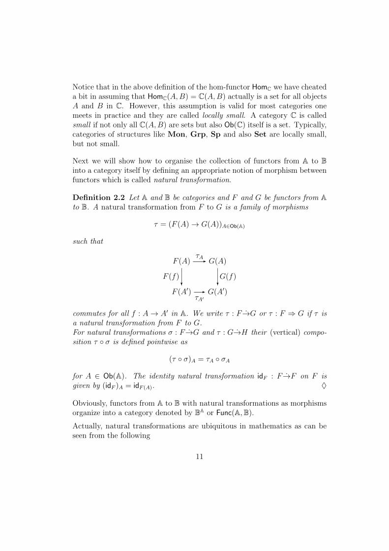
Definition 2.2 Let A and B be categories and F and G be functors from Ato B. A natural transformation from F to G is a family of morphisms

τ = (F (A)→ G(A))A∈Ob(A)

such that

F (A)τA- G(A)

F (A′)

F (f)?

τA′- G(A′)

G(f)?

commutes for all f : A→ A′ in A. We write τ : F→G or τ : F ⇒ G if τ isa natural transformation from F to G.For natural transformations σ : F→G and τ : G→H their (vertical) compo-sition τ σ is defined pointwise as

(τ σ)A = τA σA

for A ∈ Ob(A). The identity natural transformation idF : F→F on F isgiven by (idF )A = idF (A). ♦

Obviously, functors from A to B with natural transformations as morphismsorganize into a category denoted by BA or Func(A,B).

Actually, natural transformations are ubiquitous in mathematics as can beseen from the following

11

Examples of Natural Transformations

(1) Let P : Set → Set be the covariant powerset functor on Set. Thena natural transformation Id→P is given by σA : A → P(A) : a 7→a and a natural transformation from P2 = P P to P is given by⋃A : P2(A) → P(A) : X 7→

⋃X where, as usual,

⋃X is defined as

x ∈ A | ∃X ∈ X . x ∈ X.

(2) Let I be a set. Define F : Set → Set as F (X) = XI×I andF (f)(g, i) = 〈fg, i〉. Then a natural transformation ε : F → Id isgiven by εA : AI×I → A : 〈g, i〉 7→ g(i).

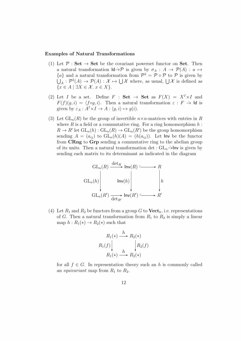
(3) Let GLn(R) be the group of invertible n×n-matrices with entries in Rwhere R is a field or a commutative ring. For a ring homomorphism h :R→ R′ let GLn(h) : GLn(R)→ GLn(R′) be the group homomorphismsending A = (aij) to GLn(h)(A) = (h(aij)). Let Inv be the functorfrom CRng to Grp sending a commutative ring to the abelian groupof its units. Then a natural transformation det : GLn→Inv is given bysending each matrix to its determinant as indicated in the diagram

GLn(R)detR- Inv(R) ⊂ - R

GLn(R′)

GLn(h)

?

detR′- Inv(R′)

Inv(h)

?⊂ - R′

h

?

(4) Let R1 and R2 be functors from a group G to Vectk, i.e. representationsof G. Then a natural transformation from R1 to R2 is simply a linearmap h : R1(∗)→ R2(∗) such that

R1(∗)h- R2(∗)

R1(∗)

R1(f)? h

- R2(∗)

R2(f)?

for all f ∈ G. In representation theory such an h is commonly calledan equivariant map from R1 to R2.

12

If σ : F→F ′ : A → B and τ : G→G′ : B → C then their horizontalcomposition τ ∗ σ : GF→G′F ′ is defined as

(τ ∗ σ)A = G′σA τFA = τF ′A GσA

where the second equality follows from τ : G→G′. We leave it as an exer-cise(!) to show that

(τ2 τ1) ∗ (σ2 σ1) = (τ2 ∗ σ2) (τ1 ∗ σ1)

for σ1 : F→F ′ and σ2 : F ′→F ′′ in Func(A,B) and τ1 : G→G′ and τ2 :G′→G′′ in Func(B,C). Moreover, one easily sees that idG ∗ idF = idGF . Thus,horizontal composition gives rise to a functor ∗ : Func(B,C)× Func(A,B)→Func(A,C) for all categories A,B,C. A category whose hom-sets themselvescarry the structure of a category such that composition is functorial are called2-categories. The category Cat of categories and functors is a 2-categorywhere Cat(A,B) is the functor category Func(A,B) and the morphism partsof the composition functors are given by horizontal composition ∗ which isfunctorial as we have seen above.One readily checks that a natural transformation τ : F→G is an isomorphismiff all its components are isomorphisms (exercise!). We say that functors Fand G from A to B are isomorphic iff there is an isomorphism from F to Gin Cat(A,B) = Func(A,B).

13

3 Subcategories, Full and Faithful Functors,

Equivalences

Though already shortly mentioned in section 1 we now “officially” give thedefinition of the notion of subcategory.

Definition 3.1 Let C be a category. A subcategory C′ of C is given by

Ob(C′) ⊆ Ob(C) and

C′(A,B) ⊆ C(A,B) for all A,B ∈ Ob(C′)

such that

i) idA ∈ C′(A,A) for all A ∈ Ob(C′)

ii) whenever f : A→ B and g : B → C are morphisms in C′ then g f isa morphism in C′

i.e. identities and composition are inherited from C.A subcategory C′ of C is called full iff C′(A,B) = C(A,B) for all A,B ∈Ob(C′) and it is called replete iff, moreover, for every isomorphism f : A→B in C the object B is in C′ whenever A is in C′. ♦

For every subcategory C′ of C there is an obvious inclusion functor

I : C′ → C

with I(A) = A and I(f) = f for all objects A and morphisms f in C′.

Definition 3.2 Let F : A→ B be a functor. The functor F is called faithfuliff for all f, g : A → B in A from F (f) = F (g) it follows that f = g, i.e.iff all morphism parts of F are one-to-one. The functor F is called full ifffor all A,B ∈ Ob(A) and g : F (A) → F (B) there is an f : A → B withg = F (f), i.e. all morphism parts of F are onto. ♦

Obviously, a functor is full and faithful iff all its morphism parts are bijec-tions.

Lemma 3.1 If a functor F : A → B is full and faithful then F reflectsisomorphisms, i.e. f is an isomorphism whenever F (f) is an isomorphism.However, in general faithful functors need not reflect isomorphisms.

14

Proof: Simple exercise(!) left to the reader.

Notice that, in particular, for subcategories C′ of C the inclusion functorI : C′ → C need not reflect isomorphisms though it always is faithful.3

Definition 3.3 A functor F : A→ B is called an equivalence (of categories)iff F is full and faithful and for every B ∈ Ob(B) there is an A ∈ A withB ∼= F (A). We write A ' B iff there is an equivalence between A and B. ♦

Notice that being an equivalence is much weaker than being an isomorphismof categories. Nevertheless equivalence is the better notion because for cate-gories isomorphism is the right notion of equality for objects.We leave it as an exercise(!) to show that (using the Axiom of Choice) forevery equivalence F : A → B there is a functor G : B → A such thatGF ∼= IdA and FG ∼= IdB, i.e. F has a “quasi-inverse” G.

3For this reason P. Freyd in his book Categories, Allegories [FS] required faithful func-tors also to reflect isomorphisms! Accordingly, he required for subcategories C′ ⊆ C alsothat f−1 is in C′ whenever f is in C′.

15

4 Comma Categories and Slice Categories

At first look the notions introduced in this section may appear as somewhatartificial. However, as we shall see later they turn out as most important forcategorical logic.

Definition 4.1 Let F : A → C and G : B → C be functors. The commacategory F↓G is defined as follows. The objects of F↓G are triples (A, f,B)where A ∈ Ob(A), B ∈ Ob(B) and f ∈ C(F (A), G(B)). A morphism from(A, f,B) to (A′, f ′, B′) in F↓G is a pair (g : A→A′, h : B→B′) such that

F (A)F (g)- F (A′)

G(B)

f?

G(h)- G(B′)

f ′?

commutes. Composition of morphisms in F↓G is componentwise, i.e. (g′, h′)(g, h) = (g′ g, h′ h) and id(A,f,B) = (idA, idB). ♦

Special cases of particular interest arise if A or B coincide with 1, the trivialcategory with one object and one morphism, or if F orG are identity functors.If G = IdC we write F↓C for F↓IdC, if F = IdC we write C↓G for IdC↓G and ifF = IdC = G then we write C↓C for IdC↓IdC. If B = 1 and G(∗) = X we writeF↓X for F↓G and if A = 1 and F (∗) = Y we write Y ↓G for F↓G. If F = IdCand G : 1 → C : ∗ 7→ X we write C/X for F↓G and if F : 1 → C : ∗ 7→ Yand G = IdC we write Y/C for F↓G. The comma category C/X is commonlycalled slice (category of C) over X.We leave it as an exercise4 to show that for all sets I we have Set/I ' SetI

where SetI is the I-fold product of Set.Notice that for categories C different from Set it always makessense to consider for I ∈ Ob(C) the slice category C/I whereas CI ismeaningless because I is not a set in this case.

4The idea is to send A ∈ SetI to the map∐

i∈I Ai −→ I : (i, a) 7→ i where as usual∐i∈I Ai = (i, a) | i∈I, a∈Ai.

16

5 Yoneda Lemma

The Yoneda lemma says that for every locally small category C there is afull and faithful functor YC : C → SetC

op

, the so-called Yoneda functor,which allows one to consider C (up to equivalence) as a full subcategory of

C = SetCop

, the category of (set-valued) presheaves over C. As we shall see

later this result is very important because categories of the form C = SetCop

are very “set-like” in the sense that they can be considered as categories of“generalised sets” and, therefore, used as models for (constructive) logic andmathematics!

Definition 5.1 (Yoneda embedding)Let C be a locally small category. For I ∈ Ob(C) the functor YC(I) : Cop →Set is defined as C(−, I), i.e. sends J ∈ Ob(C) to the set C(J, I) and sendsg : K → J to the function C(g, I) : C(J, I) → C(K, I) : h 7→ h g. Forf : I → J let YC(f) be the natural transformation from YC(I) to YC(J)whose component at K ∈ Ob(C) is given by YC(f)K : C(K, I) → C(K, J) :h 7→ f h. These data give rise to a functor YC : C → SetC

op

called theYoneda embedding for C. ♦

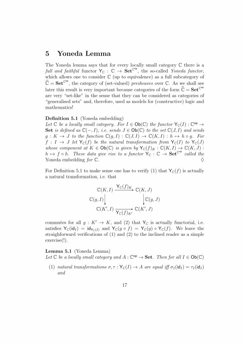
For Definition 5.1 to make sense one has to verify (1) that YC(f) is actuallya natural transformation, i.e. that

C(K, I)YC(f)K- C(K, J)

C(K ′, I)

C(g, I)?

YC(f)K′- C(K ′, J)

C(g, J)?

commutes for all g : K ′ → K, and (2) that YC is actually functorial, i.e.satisfies YC(idI) = idYC(I) and YC(g f) = YC(g) YC(f). We leave thestraighforward verifications of (1) and (2) to the inclined reader as a simpleexercise(!).

Lemma 5.1 (Yoneda Lemma)Let C be a locally small category and A : Cop → Set. Then for all I ∈ Ob(C)

(1) natural transformations σ, τ : YC(I)→ A are equal iff σI(idI) = τI(idI)and

17

(2) for every a ∈ A(I) there exists a unique natural transformation τ (a) :

YC(I)→ A with τ(a)I (idI) = a.

Accordingly, we have a natural isomorphism

ι : C(YC(−), A)∼=−→ A

given by ιI : C(YC(I), A)→ A(I) : τ 7→ τI(idI) for I ∈ C.

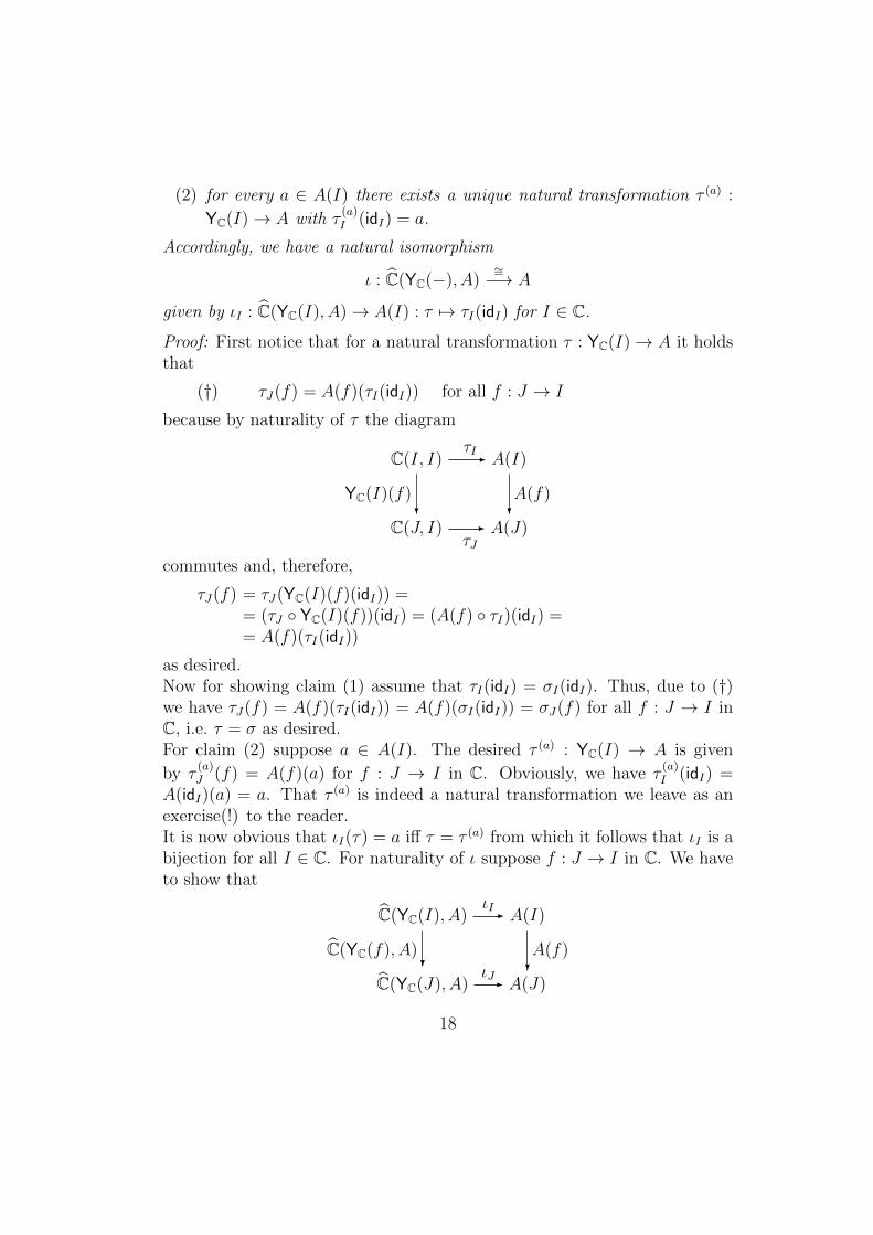
Proof: First notice that for a natural transformation τ : YC(I)→ A it holdsthat

(†) τJ(f) = A(f)(τI(idI)) for all f : J → I

because by naturality of τ the diagram

C(I, I)τI- A(I)

C(J, I)

YC(I)(f)?

τJ- A(J)

A(f)?

commutes and, therefore,

τJ(f) = τJ(YC(I)(f)(idI)) == (τJ YC(I)(f))(idI) = (A(f) τI)(idI) == A(f)(τI(idI))

as desired.Now for showing claim (1) assume that τI(idI) = σI(idI). Thus, due to (†)we have τJ(f) = A(f)(τI(idI)) = A(f)(σI(idI)) = σJ(f) for all f : J → I inC, i.e. τ = σ as desired.For claim (2) suppose a ∈ A(I). The desired τ (a) : YC(I) → A is given

by τ(a)J (f) = A(f)(a) for f : J → I in C. Obviously, we have τ

(a)I (idI) =

A(idI)(a) = a. That τ (a) is indeed a natural transformation we leave as anexercise(!) to the reader.It is now obvious that ιI(τ) = a iff τ = τ (a) from which it follows that ιI is abijection for all I ∈ C. For naturality of ι suppose f : J → I in C. We haveto show that

C(YC(I), A)ιI- A(I)

C(YC(J), A)

C(YC(f), A)?

ιJ- A(J)

A(f)?

18

commutes. Suppose τ : YC(I)→ A then we have

(A(f) ιI)(τ) = A(f)(ιI(τ)) = A(f)(τI(idI)) = (A(f) τI)(idI) == (τJ YC(I)(f))(idI) = τJ(f) = τJ(YC(f)J(idJ)) == (τ YC(f))J(idJ) = ιJ(τ YC(f)) =

= ιJ(C(YC(f), A)(τ)) =

= (ιJ C(YC(f), A))(τ)

as desired.

As the Yoneda Lemma 5.1 allows us to identify in a canonical way C(YC(I), A)

with A(I) for all presheaves A ∈ C = SetCop

we often write simply a :YC(I)→ A for the natural transformation τ (a) as constructed in the proof ofthe Yoneda lemma.

Corollary 5.1 For every locally small category C the Yoneda functor YC :C→ C is full and faithful.

Proof: We have to show that for all I, J ∈ Ob(C) and τ : YC(I) → YC(J)there exists a unique morphism f : I → J in C with τ = YC(f). Notice thatby the Yoneda Lemma 5.1 we have τK(g) = YC(J)(g)(τI(idI)) = τI(idI) gfor all g : K → I. Thus, as for f = τI(idI) we have YC(f)K(g) = f g itfollows from the Yoneda Lemma 5.1 that τ = YC(f) and f is unique withthis property.

As full and faithful functors reflect isomorphisms we get that YC(I) ∼= YC(J)implies I ∼= J and, therefore, the category C may be considered as a fullsubcategory of C. Those A : Cop → Set with A ∼= YC(I) for some I ∈Ob(C) are called representable. We give this definition an “official” statusas representability is a key concept used for defining most of the subsequentnotions.

Definition 5.2 Let C be locally small. Then A : Cop → Set is called repre-sentable iff A ∼= YC(I) for some I ∈ Ob(C). ♦

Notice that by the Yoneda lemma for representable A the representing objectI with A ∼= YC(I) is unique up to isomorphism.

19

6 Grothendieck universes : big vs. small

Generally in category theory one doesn’t worry too much about its set-theoretic foundations because one thinks that categories (namely toposes)provide a better foundation for mathematics (see e.g. [LR]).However, as we have seen in the previous section when discussing the Yonedalemma local smallness is of great importance in category theory. From thedefinition of local smallness it is evident that we want to call a collection“small” iff it is a set. Typical non-small collections are the collection of allsets or the collection of all functors from Cop to Set. Already in traditionalalgebra and topology to some extent one has to consider large collectionswhen quantifying over all groups, all topological spaces etc. In this casethe usual “excuse” is that in Zermelo-Fraenkel set theory ZF(C) one mayquantify over the universe of all sets and, therefore, also over collectionswhich can be expressed by a predicate in the language of set theory (i.e. afirst order formula using only the binary predicates = and ∈). In Godel-Bernays-vonNeumann class theory GBN one may even give an “ontologicalstatus” to such collections which usually are referred to as classes.5 Thedrawback, however, is that classes don’t enjoy good closure properties, e.g.there doesn’t exist the class of all functions from class X to class Y etc.Thus, the desire to freely manipulate big collections has driven categoriststo introduce the following notion of universe.

Definition 6.1 A Grothendieck universe is a set U such that the followingproperties

(U1) if x ∈ a ∈ U then x ∈ U(U2) if a, b ∈ U then a, b and a×b are elements of U(U3) if a ∈ U then

⋃a and P(a) are elements of U

(U4) the set ω of all natural numbers is an element of U(U5) if f : a→ b is surjective with a ∈ U and b ⊆ U then b ∈ U

hold for U . ♦

Notice that the conditions (U1)–(U5) guarantee that U with ∈ restricted to

5For a first order formula φ(x) in the language of set theory one may form the classx | φ(x) consisting of all sets a satisfying φ(a) (where a set is a class contained in someclass (e.g. x | x = x) as an element).

20

U×U provides a model for ZF(C) (i.e. a “small inner model”6 in the slangof set theory). Thus, the universe U is closed under the usual set-theoreticoperations.7

Notice, however, that ZF(C) cannot prove the existence of Grothendieckuniverses as otherwise ZF(C) could prove its own consistency in contradictionto Godel’s second incompleteness theorem. Nevertheless, one shouldn’t betoo afraid of inconsistencies when postulating Grothendieck universes as itis nothing but a reflection principle claiming that what we have axiomatizedin ZF(C) “actually exists”. In other words, if ZF(C) + the assumption of aGrothendieck universe were inconsistent then it were rather the fault of theformer8 than the fault of the latter.If having accepted one Grothendieck universe why shouldn’t one acceptmore? Accordingly, when really worrying about set-theoretic foundationsfor category theory one usually adds to ZF(C) the requirement that for ev-ery set a there is a Grothendieck universe U with a ∈ U . Accordingly,for every Grothendieck universe U there is a Grothendieck universe U ′ withU ∈ U ′ and, therefore, also U ⊆ U ′. Thus, this axiomatic setting guarantees(at least) the existence9 of a hierarchy U0 ∈ U1 ∈ · · · ∈ Un ∈ Un+1 ∈ · · · ofuniverses which is also cumulative in the sense that U0 ⊆ U1 ⊆ · · · ⊆ Un ⊆Un+1 ⊆ · · · holds as well.

In the rest of these notes we will not refer anymore to the set-theoretical sophistications discussed in this section but, instead,will use the notions “big” and “small” informally.

6Actually, the notion of universe is somewhat stronger than that of a small inner modelas the latter need not satisfy (U5) for arbirary functions f but only for first order definablef as ensured by the set theoretic replacement axiom.

7We suggest it as an exercise(!) to directly derive from conditions (U1)–(U5) that〈a, b〉 = a, a, b ∈ U whenever a, b ∈ U .

8What makes ZF so incredibly strong is the mixture of infinity, powersets and thereplacement axiom!

9Notice that in presence of the axiom of choice such a cumulative hierarchy canbe constructed internally by iterating the choice function u assigning to every set a aGrothendieck universe u(a) with a ∈ u(a). Of course, nothing prevents us from iteratingthis function u along arbitrary transfinite ordinals!

21

7 Limits and Colimits

A lot of important properties of categories can be formulated by requiringthat limits or colimits of a certain kind do exist meaning that certain functorsare representable.Before introducing the general notion of limit and colimit for a diagram westudy some particular instances of these notions which, however, togetherwill guarantee that all (small) limits (or colimits) do exist.

Definition 7.1 (cartesian products)Let C be a category. The (cartesian) product of a family A = (Ai | i ∈ I)of objects in C is given by an object P of C together with a family π = (πi :P → Ai | i ∈ I) of morphisms in C such that for every object C and everyfamily f = (fi : C → Ai | i ∈ I) there exists a unique morphism g : C → Pwith fi = πig for all i ∈ I. This unique morphism g will often be denoted as〈fi〉i∈I and is called the mediating arrow from f to π. The object P togetherwith the family π is called product cone over A and πi : P → Ai is calledi-th projection. ♦

Next we will show that product cones are unique up to isomorphism.

Lemma 7.1 Suppose π = (πi : P → Ai | i ∈ I) and π′ = (π′i : P ′ → Ai |i ∈ I) are product cones over A = (Ai | i ∈ I). Then for the unique arrowsf : P → P ′ and g : P ′ → P such that π′i f = πi and πi g = π′i for all i ∈ Iit holds that g f = idP and f g = idP ′, i.e. that the cones π and π′ arecanonically isomorphic.

Proof: Due to our assumptions we have that for all i ∈ I it holds that

πi g f = π′i f = πi

and, therefore, by uniqueness of mediating arrows idP = g f (becauseπi idP = πi for all i ∈ I). Similarly one shows that f g = idP ′ .

Notice that for I = ∅ a product cone (P, π) over (Ai | i ∈ I) is alreadydetermined by the object P (because π has to be the empty family) whichhas to satisfy the condition that for every object C ∈ Ob(C) there is aunique morphism from C to P . Such objects P will be called terminal andare usually denoted as T or 1.

22

Definition 7.2 (terminal objects)An object T in C is called terminal iff for every C ∈ Ob(C) there is a uniquemorphism C → T in C (often denoted as !C). ♦

In Set a product cone for A = (Ai | i ∈ I) is given by P =∏

i∈I Ai where∏i∈I

Ai = s : I →⋃i∈I

Ai | ∀i ∈ I. s(i) ∈ Ai

and π = (πi | i ∈ I) with πi(s) = s(i).Terminal objects in Set are those sets containing precisely one element. Ac-cordingly, we often write 1 for a terminal object.We recommend it as an exercise(!) to construct products in the categoriesMon, Sp etc.

Definition 7.3 (equalisers) Let f, g : A→ B in C. An equaliser of f and gis a morphism e : E → A such that

(i) f e = g e and

(ii) for every h : C → A with f h = g h there exists a unique morphismk : C → E with h = e k. ♦

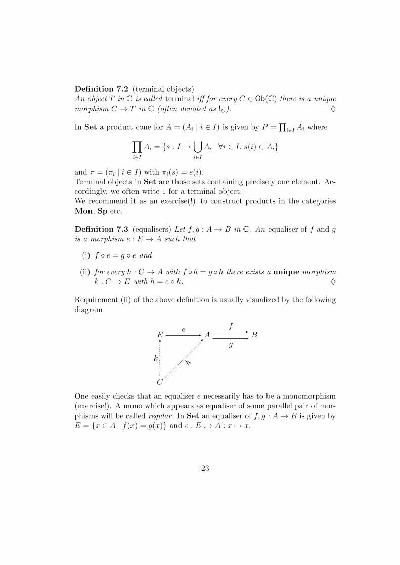
Requirement (ii) of the above definition is usually visualized by the followingdiagram

Ee- A

f-

g- B

C

k

6.................

h

-

One easily checks that an equaliser e necessarily has to be a monomorphism(exercise!). A mono which appears as equaliser of some parallel pair of mor-phisms will be called regular. In Set an equaliser of f, g : A→ B is given byE = x ∈ A | f(x) = g(x) and e : E → A : x 7→ x.

23

Definition 7.4 (small/finitely complete)A category C has (small) limits iff C has products of (small) families ofobjects and C has equalisers.A category C has finite limits iff C has finite products (i.e. products for finitefamilies of objects) and C has equalisers.A category C is small/finitely complete iff C has finite/small limits. ♦

Obviously, a category C has finite limits iff C has a terminal object, binaryproducts and equalisers (exercise!).Next we consider the most important case of pullbacks which exist in allcategories with finite limits. Moreover, we will see that categories with aterminal object and all pullbacks will also have all finite limits.

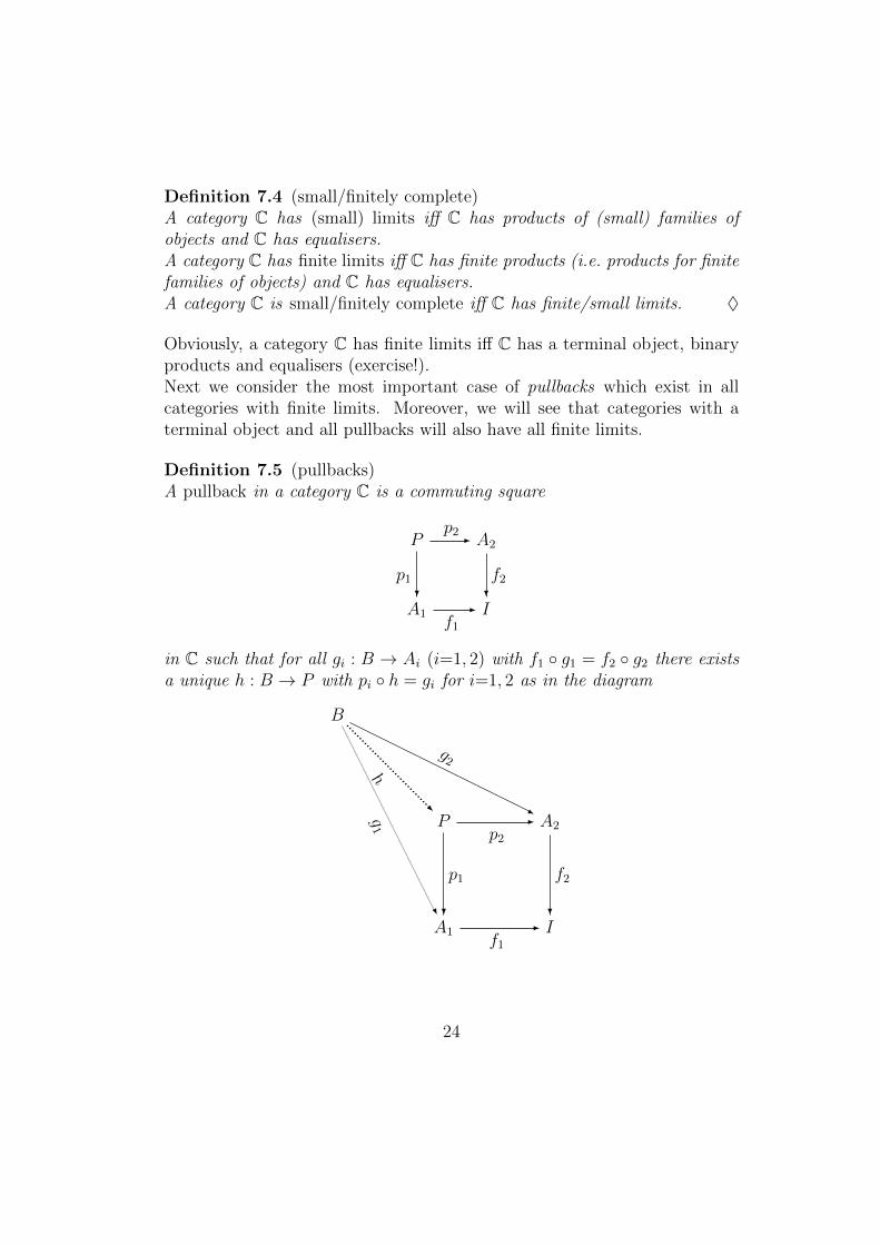
Definition 7.5 (pullbacks)A pullback in a category C is a commuting square

Pp2- A2

A1

p1?

f1

- I

f2?

in C such that for all gi : B → Ai (i=1, 2) with f1 g1 = f2 g2 there existsa unique h : B → P with pi h = gi for i=1, 2 as in the diagram

B

Pp2

-

.................................

h-

A2

g2

-

A1

p1

?

f1

-

g1

-

I

f2

?

24

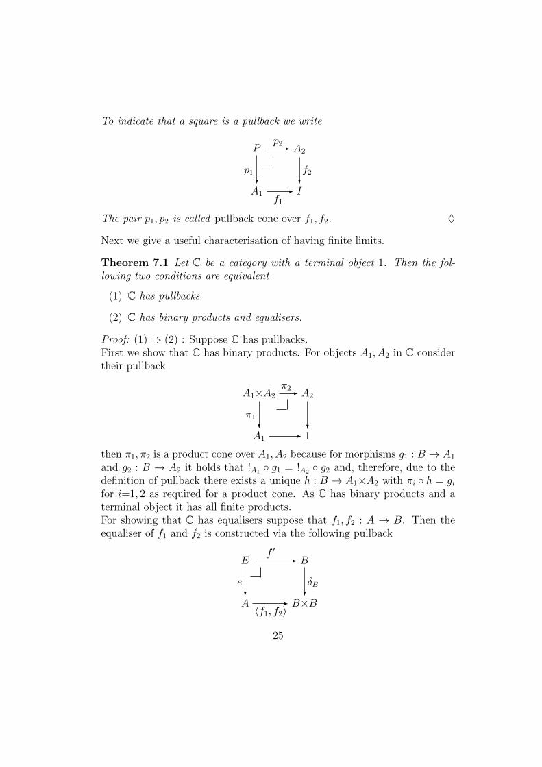
To indicate that a square is a pullback we write

Pp2- A2

A1

p1?

f1

- I

f2?

The pair p1, p2 is called pullback cone over f1, f2. ♦

Next we give a useful characterisation of having finite limits.

Theorem 7.1 Let C be a category with a terminal object 1. Then the fol-lowing two conditions are equivalent

(1) C has pullbacks

(2) C has binary products and equalisers.

Proof: (1)⇒ (2) : Suppose C has pullbacks.First we show that C has binary products. For objects A1, A2 in C considertheir pullback

A1×A2

π2- A2

A1

π1?

- 1?

then π1, π2 is a product cone over A1, A2 because for morphisms g1 : B → A1

and g2 : B → A2 it holds that !A1 g1 = !A2 g2 and, therefore, due to thedefinition of pullback there exists a unique h : B → A1×A2 with πi h = gifor i=1, 2 as required for a product cone. As C has binary products and aterminal object it has all finite products.For showing that C has equalisers suppose that f1, f2 : A → B. Then theequaliser of f1 and f2 is constructed via the following pullback

Ef ′

- B

A

e?

〈f1, f2〉- B×B

δB?

25

where δB = 〈idB, idB〉. The morphism e equalises f1 and f2 because we have

fi e = πi 〈f1, f2〉 e = πi δB f ′ = idB f ′ = f ′

for i=1, 2 and, accordingly, that f1 e = f2 e. Now suppose g : C → A withf1 g = f2 g for which morphism we write g′. As for i=1, 2 we have

πi δB g′ = g′ = fi g = πi 〈f1, f2〉 g

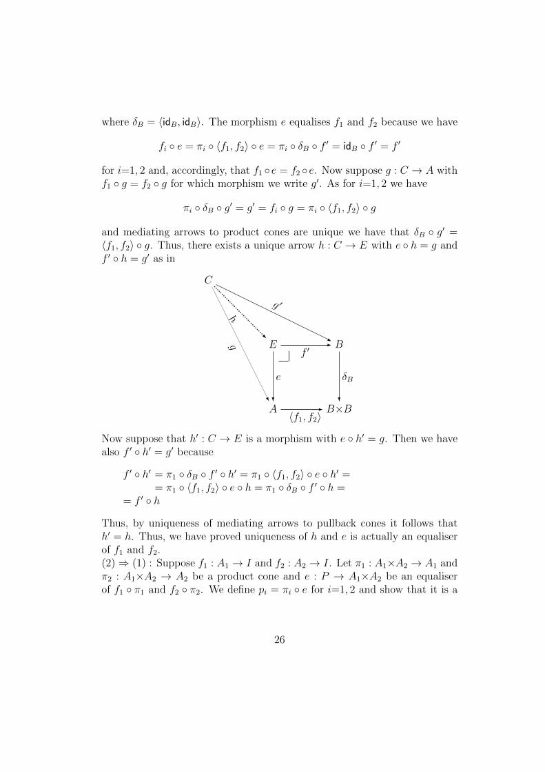
and mediating arrows to product cones are unique we have that δB g′ =〈f1, f2〉 g. Thus, there exists a unique arrow h : C → E with e h = g andf ′ h = g′ as in

C

Ef ′

-

.................................

h-

B

g ′

-

A

e

?

〈f1, f2〉-

g

-

B×B

δB

?

Now suppose that h′ : C → E is a morphism with e h′ = g. Then we havealso f ′ h′ = g′ because

f ′ h′ = π1 δB f ′ h′ = π1 〈f1, f2〉 e h′ == π1 〈f1, f2〉 e h = π1 δB f ′ h =

= f ′ h

Thus, by uniqueness of mediating arrows to pullback cones it follows thath′ = h. Thus, we have proved uniqueness of h and e is actually an equaliserof f1 and f2.(2)⇒ (1) : Suppose f1 : A1 → I and f2 : A2 → I. Let π1 : A1×A2 → A1 andπ2 : A1×A2 → A2 be a product cone and e : P → A1×A2 be an equaliserof f1 π1 and f2 π2. We define pi = πi e for i=1, 2 and show that it is a

26

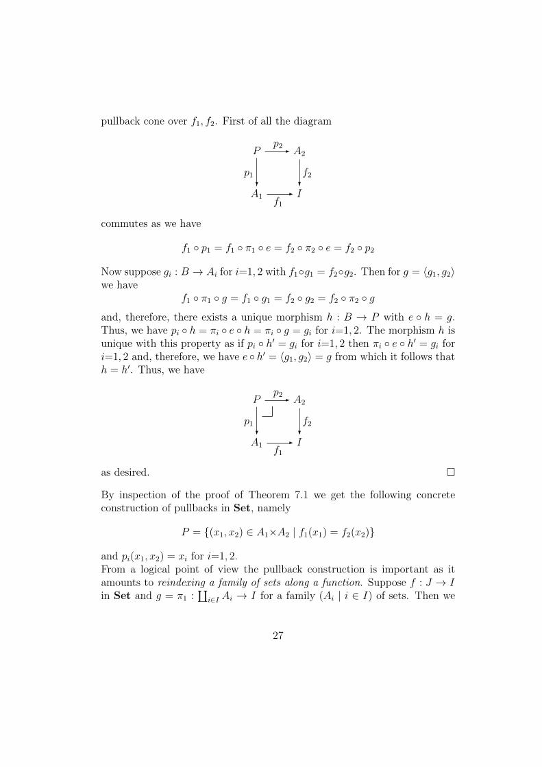
pullback cone over f1, f2. First of all the diagram

Pp2- A2

A1

p1?

f1

- I

f2?

commutes as we have

f1 p1 = f1 π1 e = f2 π2 e = f2 p2

Now suppose gi : B → Ai for i=1, 2 with f1g1 = f2g2. Then for g = 〈g1, g2〉we have

f1 π1 g = f1 g1 = f2 g2 = f2 π2 g

and, therefore, there exists a unique morphism h : B → P with e h = g.Thus, we have pi h = πi e h = πi g = gi for i=1, 2. The morphism h isunique with this property as if pi h′ = gi for i=1, 2 then πi e h′ = gi fori=1, 2 and, therefore, we have e h′ = 〈g1, g2〉 = g from which it follows thath = h′. Thus, we have

Pp2- A2

A1

p1?

f1

- I

f2?

as desired.

By inspection of the proof of Theorem 7.1 we get the following concreteconstruction of pullbacks in Set, namely

P = (x1, x2) ∈ A1×A2 | f1(x1) = f2(x2)

and pi(x1, x2) = xi for i=1, 2.From a logical point of view the pullback construction is important as itamounts to reindexing a family of sets along a function. Suppose f : J → Iin Set and g = π1 :

∐i∈I Ai → I for a family (Ai | i ∈ I) of sets. Then we

27

have ∐j∈J

Af(j)

q-∐i∈I

Ai

J

π1

?

f- I

π1

?

where q(j, x) = (f(j), x) as follows from the obvious 1-1-correspondence be-tween pairs (j, x) ∈

∐j∈J Af(j) and tuples (j, (i, x)) with i = f(j) and x ∈ Ai.

Having seen how to compute pullbacks in Set we recommend it as an exer-cise(!) to construct pullbacks in the categories Mon, Grp, Sp etc.

By dualisation for every kind of limit there is a dual notion of colimit assummarised in the following table

C Cop

sum productcoequaliser equaliserpushout pullbackinitial object terminal object

We recommend it as an exercise(!) to show that Set has the above mentionedcolimits. What about Mon, Grp, Sp etc.?

Because of their great importance for reasoning about pullbacks we provethe following lemmata.

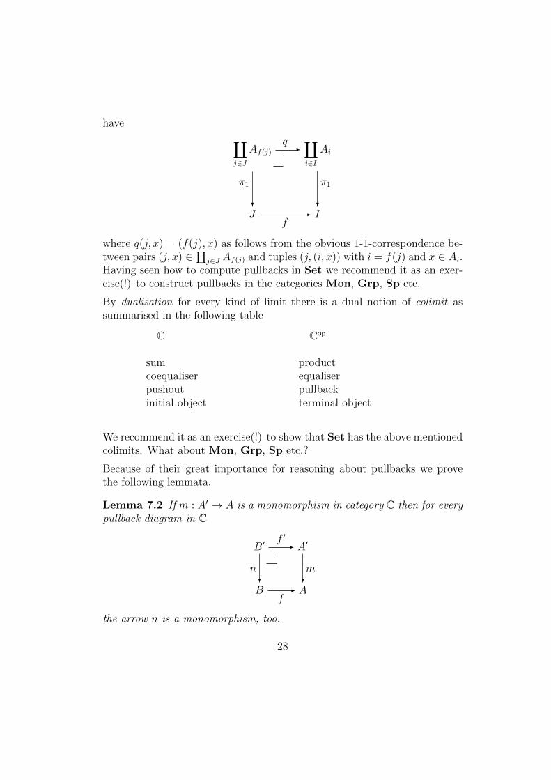
Lemma 7.2 If m : A′ → A is a monomorphism in category C then for everypullback diagram in C

B′f ′- A′

B

n?

f- A

m?

the arrow n is a monomorphism, too.

28

Proof: Suppose g1, g2 : C → B′ with n g1 = n g2. Then we also havef ′ g1 = f ′ g2 because m f ′ g1 = f n g1 = f n g2 = m f ′ g2 andm is a mono by assumption. Thus, it follows that g1 = g2 by uniqueness ofmediating arrows.

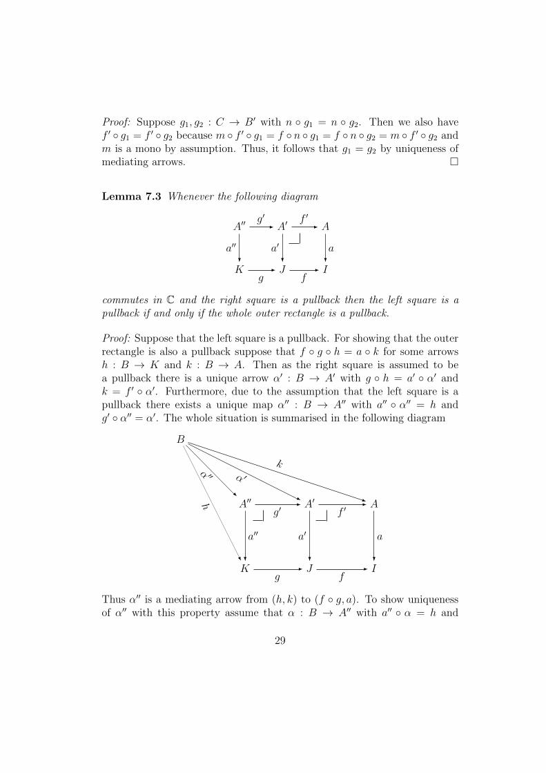
Lemma 7.3 Whenever the following diagram

A′′g′- A′

f ′- A

K

a′′

?

g- J

a′

?

f- I

a?

commutes in C and the right square is a pullback then the left square is apullback if and only if the whole outer rectangle is a pullback.

Proof: Suppose that the left square is a pullback. For showing that the outerrectangle is also a pullback suppose that f g h = a k for some arrowsh : B → K and k : B → A. Then as the right square is assumed to bea pullback there is a unique arrow α′ : B → A′ with g h = a′ α′ andk = f ′ α′. Furthermore, due to the assumption that the left square is apullback there exists a unique map α′′ : B → A′′ with a′′ α′′ = h andg′ α′′ = α′. The whole situation is summarised in the following diagram

B

A′′g′-

α ′′-

A′f ′

-

α ′

-A

k

-

K

a′′

?

g-

h

-

J

a′

?

f- I

a

?

Thus α′′ is a mediating arrow from (h, k) to (f g, a). To show uniquenessof α′′ with this property assume that α : B → A′′ with a′′ α = h and

29

f ′ g′ α = k. But then we have also that a′ g′ α = g a′′ α = g hand, therefore, it follows that α′ = g′ α by uniqueness of mediating arrows.Thus, again by uniqueness of mediating arrows it follows that α = α′′.

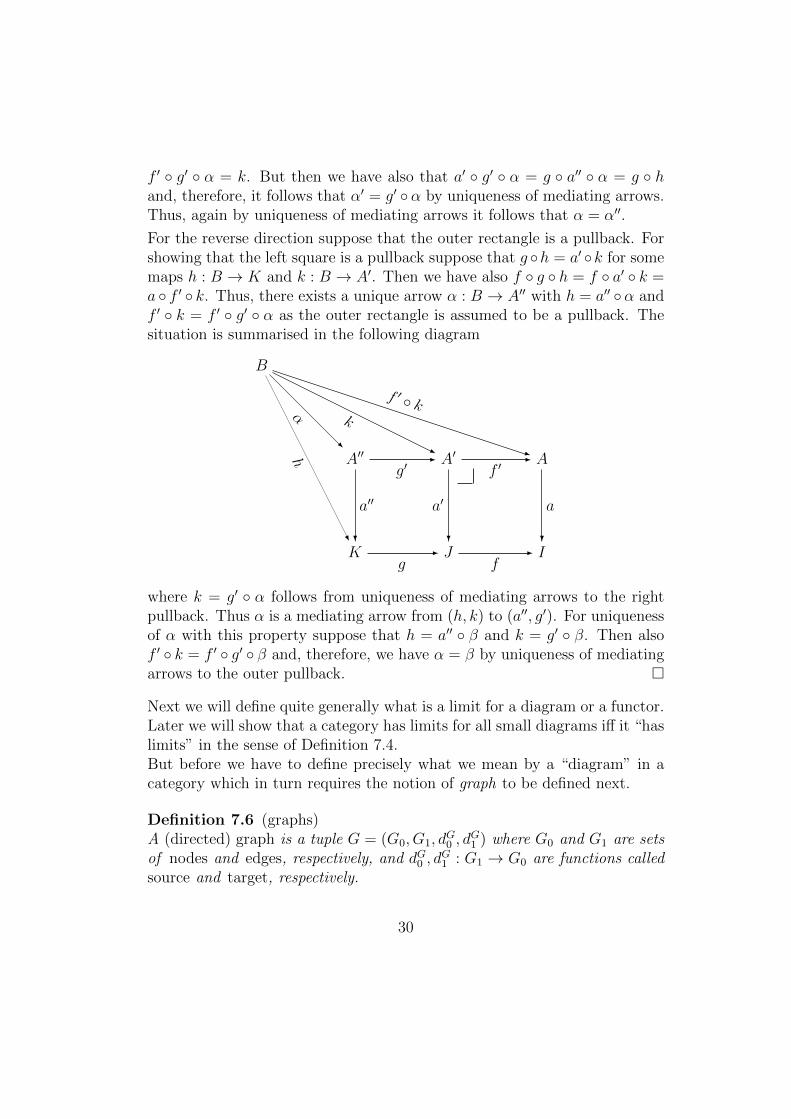
For the reverse direction suppose that the outer rectangle is a pullback. Forshowing that the left square is a pullback suppose that g h = a′ k for somemaps h : B → K and k : B → A′. Then we have also f g h = f a′ k =a f ′ k. Thus, there exists a unique arrow α : B → A′′ with h = a′′ α andf ′ k = f ′ g′ α as the outer rectangle is assumed to be a pullback. Thesituation is summarised in the following diagram

B

A′′g′-

α

-

A′f ′

-

k

-A

f ′ k

-

K

a′′

?

g-

h

-

J

a′

?

f- I

a

?

where k = g′ α follows from uniqueness of mediating arrows to the rightpullback. Thus α is a mediating arrow from (h, k) to (a′′, g′). For uniquenessof α with this property suppose that h = a′′ β and k = g′ β. Then alsof ′ k = f ′ g′ β and, therefore, we have α = β by uniqueness of mediatingarrows to the outer pullback.

Next we will define quite generally what is a limit for a diagram or a functor.Later we will show that a category has limits for all small diagrams iff it “haslimits” in the sense of Definition 7.4.But before we have to define precisely what we mean by a “diagram” in acategory which in turn requires the notion of graph to be defined next.

Definition 7.6 (graphs)A (directed) graph is a tuple G = (G0, G1, d

G0 , d

G1 ) where G0 and G1 are sets

of nodes and edges, respectively, and dG0 , dG1 : G1 → G0 are functions called

source and target, respectively.

30

For graphs G and H a graph morphism from G to H is given by a pairf = (f0, f1) where fi : Gi → Hi for i=0, 1 satisfying

dHi f1 = f0 dGifor i=0, 1. ♦

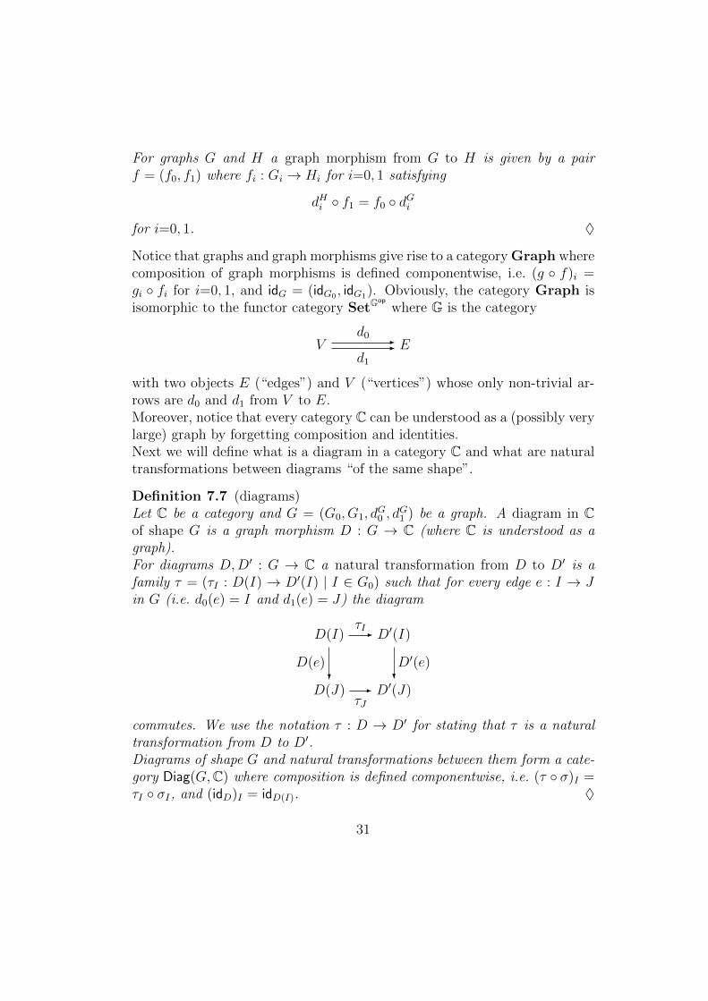
Notice that graphs and graph morphisms give rise to a category Graph wherecomposition of graph morphisms is defined componentwise, i.e. (g f)i =gi fi for i=0, 1, and idG = (idG0 , idG1). Obviously, the category Graph isisomorphic to the functor category SetG

op

where G is the category

Vd0 -

d1

- E

with two objects E (“edges”) and V (“vertices”) whose only non-trivial ar-rows are d0 and d1 from V to E.Moreover, notice that every category C can be understood as a (possibly verylarge) graph by forgetting composition and identities.Next we will define what is a diagram in a category C and what are naturaltransformations between diagrams “of the same shape”.

Definition 7.7 (diagrams)Let C be a category and G = (G0, G1, d

G0 , d

G1 ) be a graph. A diagram in C

of shape G is a graph morphism D : G → C (where C is understood as agraph).For diagrams D,D′ : G → C a natural transformation from D to D′ is afamily τ = (τI : D(I) → D′(I) | I ∈ G0) such that for every edge e : I → Jin G (i.e. d0(e) = I and d1(e) = J) the diagram

D(I)τI- D′(I)

D(J)

D(e)?

τJ- D′(J)

D′(e)?

commutes. We use the notation τ : D → D′ for stating that τ is a naturaltransformation from D to D′.Diagrams of shape G and natural transformations between them form a cate-gory Diag(G,C) where composition is defined componentwise, i.e. (τ σ)I =τI σI , and (idD)I = idD(I). ♦

31

In order to formulate a notion of limit for diagrams of shape G we need asan auxiliary notion a functor ∆G

C from C to Diag(G,C) assigning to everyobject X in C “the constant diagram in C of shape G with value X”.

Definition 7.8 Let C be a category and G a graph. Then the functor ∆GC :

C→ Diag(G,C) sends an object X ∈ Ob(C) to the diagram ∆GC(X) with

∆GC(X)(I) = X for I ∈ G0 and

∆GC(X)(e) = idX for e ∈ G1

and a morphism f : X → Y in C to the natural transformation ∆GC(f) :

∆GC(X)→ ∆G

C(Y ) with ∆GC(f)I = f for I ∈ G0. ♦

Now we are ready to define what is a limit cone for a diagram D : G→ C.

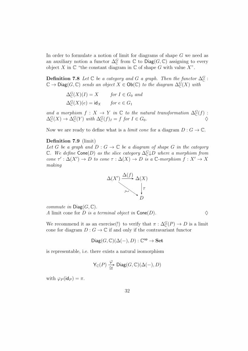
Definition 7.9 (limit)Let G be a graph and D : G → C be a diagram of shape G in the categoryC. We define Cone(D) as the slice category ∆G

C↓D where a morphism fromcone τ ′ : ∆(X ′) → D to cone τ : ∆(X) → D is a C-morphism f : X ′ → Xmaking

∆(X ′)∆(f)- ∆(X)

D

τ?

τ ′ -

commute in Diag(G,C).A limit cone for D is a terminal object in Cone(D). ♦

We recommend it as an exercise(!) to verify that π : ∆GC(P ) → D is a limit

cone for diagram D : G→ C if and only if the contravariant functor

Diag(G,C)(∆(−), D) : Cop → Set

is representable, i.e. there exists a natural isomorphism

YC(P )ϕ∼=- Diag(G,C)(∆(−), D)

with ϕP (idP ) = π.

32

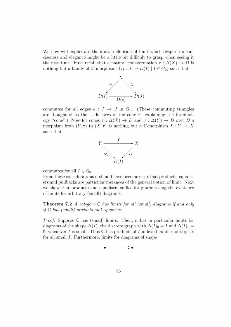
We now will explicitate the above definition of limit which despite its con-ciseness and elegance might be a little bit difficult to grasp when seeing itthe first time. First recall that a natural transformation τ : ∆(X) → D isnothing but a family of C-morphisms (τI : X → D(I) | I ∈ G0) such that

X

D(I)D(e)

-

τ I

D(J)

τJ

-

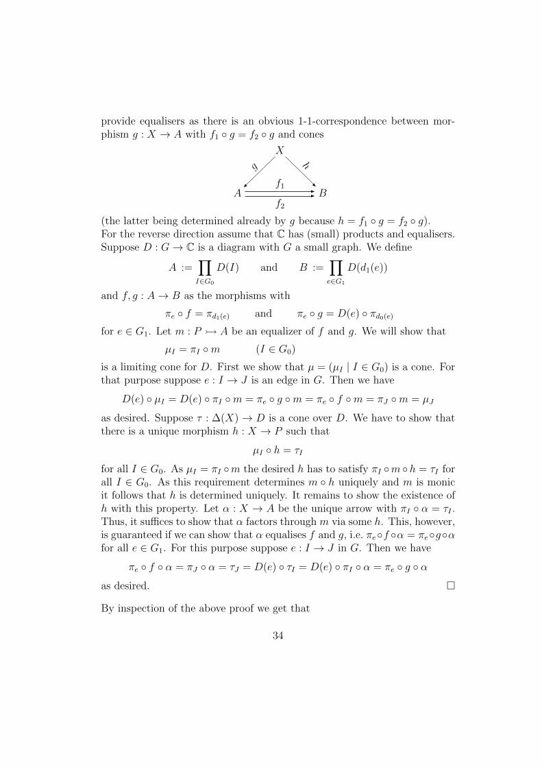
commutes for all edges e : I → J in G1. (These commuting trianglesare thought of as the “side faces of the cone τ” explaining the terminol-ogy “cone”.) Now for cones τ : ∆(X) → D and σ : ∆(Y ) → D over D amorphism from (Y, σ) to (X, τ) is nothing but a C-morphism f : Y → Xsuch that

Yf

- X

D(I) τ I

σI -

commutes for all I ∈ G0.From these considerations it should have become clear that products, equalis-ers and pullbacks are particular instances of the general notion of limit. Nextwe show that products and equalisers suffice for guaranteeing the existenceof limits for arbitrary (small) diagrams.

Theorem 7.2 A category C has limits for all (small) diagrams if and onlyif C has (small) products and equalisers.

Proof: Suppose C has (small) limits. Then, it has in particular limits fordiagrams of the shape ∆(I), the discrete graph with ∆(I)0 = I and ∆(I)1 =∅, whenever I is small. Thus C has products of I-indexed families of objectsfor all small I. Furthermore, limits for diagrams of shape

• -- •

33

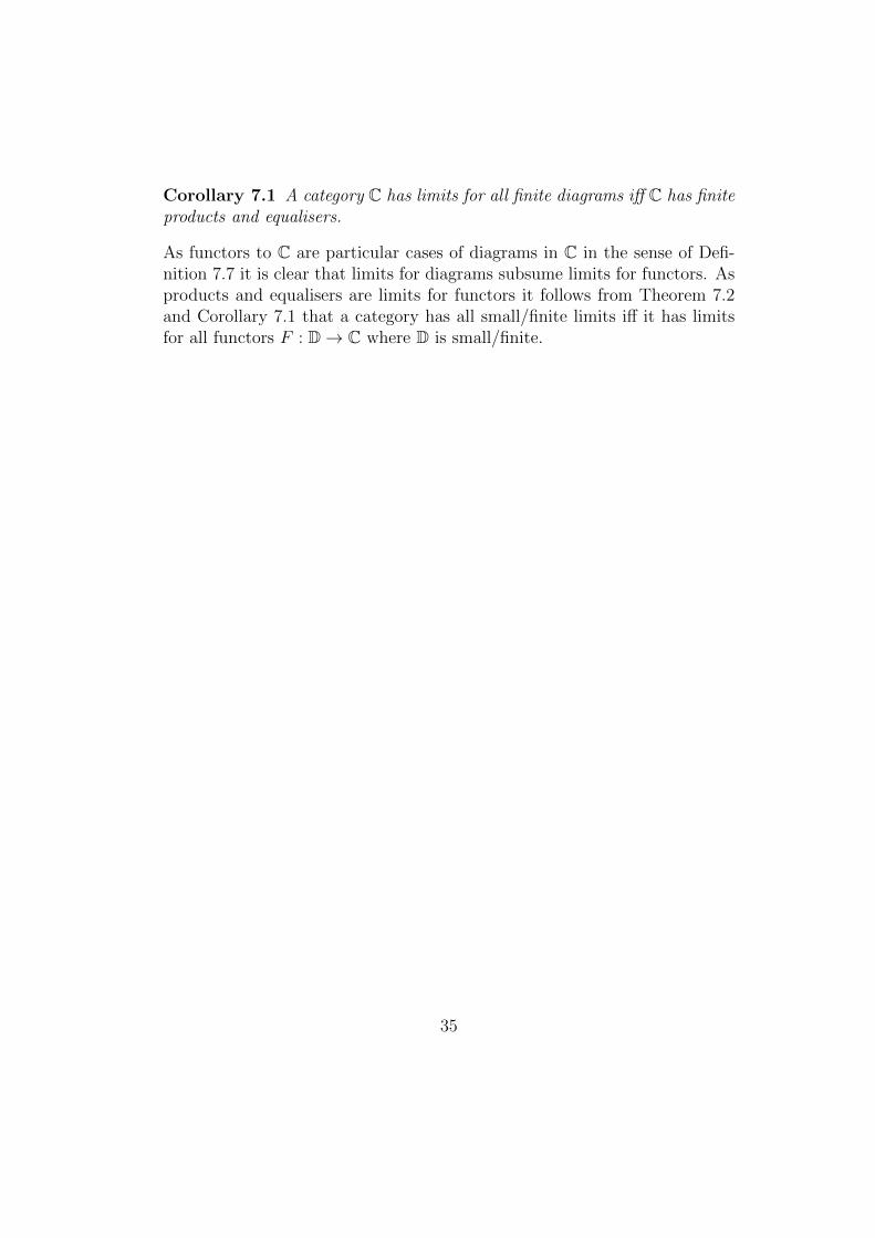
provide equalisers as there is an obvious 1-1-correspondence between mor-phism g : X → A with f1 g = f2 g and cones

X

Af1 -

f2

-

g

B

h

-

(the latter being determined already by g because h = f1 g = f2 g).For the reverse direction assume that C has (small) products and equalisers.Suppose D : G→ C is a diagram with G a small graph. We define

A :=∏I∈G0

D(I) and B :=∏e∈G1

D(d1(e))

and f, g : A→ B as the morphisms with

πe f = πd1(e) and πe g = D(e) πd0(e)

for e ∈ G1. Let m : P A be an equalizer of f and g. We will show that

µI = πI m (I ∈ G0)

is a limiting cone for D. First we show that µ = (µI | I ∈ G0) is a cone. Forthat purpose suppose e : I → J is an edge in G. Then we have

D(e) µI = D(e) πI m = πe g m = πe f m = πJ m = µJ

as desired. Suppose τ : ∆(X)→ D is a cone over D. We have to show thatthere is a unique morphism h : X → P such that

µI h = τI

for all I ∈ G0. As µI = πI m the desired h has to satisfy πI m h = τI forall I ∈ G0. As this requirement determines m h uniquely and m is monicit follows that h is determined uniquely. It remains to show the existence ofh with this property. Let α : X → A be the unique arrow with πI α = τI .Thus, it suffices to show that α factors through m via some h. This, however,is guaranteed if we can show that α equalises f and g, i.e. πef α = πegαfor all e ∈ G1. For this purpose suppose e : I → J in G. Then we have

πe f α = πJ α = τJ = D(e) τI = D(e) πI α = πe g α

as desired.

By inspection of the above proof we get that

34

Corollary 7.1 A category C has limits for all finite diagrams iff C has finiteproducts and equalisers.

As functors to C are particular cases of diagrams in C in the sense of Defi-nition 7.7 it is clear that limits for diagrams subsume limits for functors. Asproducts and equalisers are limits for functors it follows from Theorem 7.2and Corollary 7.1 that a category has all small/finite limits iff it has limitsfor all functors F : D→ C where D is small/finite.

35

8 Adjoint Functors

Because of its great importance for our treatment of adjoint functors werecall the notion of representable presheaf and give a simple characterisationof representability.

Theorem 8.1 (characterisation of representability)Let C be a (small) category. Then

(1) a (contravariant) presheaf F : Cop → Set is representable, i.e. iso-morphic to YC(I) = C(−, I) for some I ∈ Ob(C), iff there exists anx ∈ F (I) such that for every y ∈ F (J) there exists a unique morphismu : J → I in C with y = F (u)(x)

(2) a (covariant) presheaf F : C → Set is representable, i.e. isomorphicto C(I,−) for some I ∈ Ob(C), iff there exists an x ∈ F (I) such thatfor all y ∈ F (J) there exists a unique morphism u : I → J in C withy = F (u)(x).

Proof: We just prove (1) and leave the (analogous) argument for (2) to thereader as an exercise(!).Suppose F is representable, i.e. there exists a natural isomorphism ϕ :

YC(I)∼=→ F . Then x = ϕI(idI) ∈ F (I) has the desired property as for

y ∈ F (J) the morphism ϕ−1J (y) is the unique arrow u : J → I with

y = F (u)(x) which can be seen as follows. We have

F (u)(x) = F (u)(ϕI(idI)) = ϕJ(YC(I)(u)(idI)) = ϕJ(u) = ϕJ(ϕ−1J (y)) = y

and if y = F (v)(x) then

ϕ−1J (y) = ϕ−1

J (F (v)(x)) = YC(I)(v)(ϕ−1I (x)) = YC(I)(v)(idI) = idI v = v .

For the reverse direction suppose that x ∈ F (I) such that for every y ∈F (J) there exists a unique u : J → I with y = F (u)(x). Then by theYoneda lemma there exists a unique natural transformation ϕ : YC(I) →F with ϕI(idI) = x. From the proof of the Yoneda lemma we know thatϕJ(u) = F (u)(x). Thus, due to our assumption about x we know that ϕJ isa bijection for all J ∈ Ob(C) and, therefore, the natural transformation ϕ is

an isomorphism in C.

36

Definition 8.1 (category of elements)Let C be a (small) category.

(1) For a (contravariant) presheaf F : Cop → Set its category of ele-ments Elts(F ) is defined as follows: its objects are pairs (I, x) ∈∐

I∈Ob(C) F (I), its morphisms from (J, y) to (I, x) are the C-morphisms

u : J → I with y = F (u)(x) and composition and identities are inher-ited from C.

(2) For a (covariant) presheaf F : C → Set its category of elementsElts(F ) is defined as follows: its objects are pairs (I, x) ∈

∐I∈Ob(C) F (I),

its morphisms from (I, x) to (J, y) are the C-morphisms u : I → J withy = F (u)(x) and composition and identities are inherited from C. ♦

Notice that for a contravariant presheaf F : Cop → Set the category Elts(F )is isomorphic to the comma category F op↓1 (where F op : C → Setop). Sim-ilarly, for a covariant presheaf F : C → Set the category Elts(F ) is iso-morphic to 1↓F . Alternatively, for a contravariant presheaf F : Cop → Setthe category Elts(F ) is isomorphic to YC↓F and for a covariant presheafF : C → Set the category Elts(F ) is isomorphic to (YCop↓F )op. The verifi-cation of these claims we leave to the reader as an exercise(!).

Using the terminology of Definition 8.1 we can reformulate Theorem 8.1 quiteelegantly as follows.

Theorem 8.2 Let C be a small category. Then F : Cop → Set is repre-sentable iff Elts(F ) has a terminal object and F : C→ Set is representableiff Elts(F ) has an initial object.

Proof: We prove the claim just for contravariant F . For covariant F theargument is analogous by duality.By Theorem 8.1 F is representable iff there exists an x ∈ F (I) such that forevery y ∈ F (J) there is a unique arrow u : J → I with y = F (u)(x), i.e.iff (I, x) is terminal in Elts(F ). Thus F is representable iff Elts(F ) has aterminal object.

Based on the notion of representability we are ready to define the notion ofadjointness.

37

Definition 8.2 (left and right adjointable)A functor F : A→ B is called right adjointable iff for every B ∈ Ob(B) thefunctor YB(B) F op = B(F (−), B) : Aop → Set is representable.A functor U : B → A is called left adjointable iff for all A ∈ Ob(A) thefunctor A(A,U(−)) : B→ Set is representable. ♦

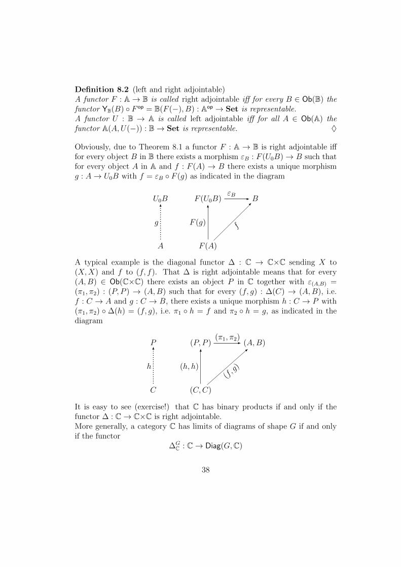
Obviously, due to Theorem 8.1 a functor F : A → B is right adjointable ifffor every object B in B there exists a morphism εB : F (U0B)→ B such thatfor every object A in A and f : F (A) → B there exists a unique morphismg : A→ U0B with f = εB F (g) as indicated in the diagram

U0B F (U0B)εB - B

A

g

6................

F (A)

F (g)

6

f

-

A typical example is the diagonal functor ∆ : C → C×C sending X to(X,X) and f to (f, f). That ∆ is right adjointable means that for every(A,B) ∈ Ob(C×C) there exists an object P in C together with ε(A,B) =(π1, π2) : (P, P ) → (A,B) such that for every (f, g) : ∆(C) → (A,B), i.e.f : C → A and g : C → B, there exists a unique morphism h : C → P with(π1, π2) ∆(h) = (f, g), i.e. π1 h = f and π2 h = g, as indicated in thediagram

P (P, P )(π1, π2)

- (A,B)

C

h

6.................

(C,C)

(h, h)

6

(f, g

)

-

It is easy to see (exercise!) that C has binary products if and only if thefunctor ∆ : C→ C×C is right adjointable.More generally, a category C has limits of diagrams of shape G if and onlyif the functor

∆GC : C→ Diag(G,C)

38

is right adjointable, i.e.

limD ∆GC(limD)

π- D

X

h

6.................

∆GC(X)

∆GC(h)

6

τ

-

A further example, particularly interesting from a “logical” point of view,is the following characterisation of function spaces. Let A be a set. Thenthe functor (−)×A : Set → Set (sending f : Y → X to f×A : Y×A →X×A : (y, a) 7→ (f(y), a)) is right adjointable, i.e. there exists a set BA

together with a map ε : BA×A→ B such that for every f : C×A→ B thereexists a unique map g : C → BA with ε (g×A) = f . Naturally for BA

one chooses the set of all functions from A to B and defines ε : BA×A→ Bas the evaluation map sending (f, a) to f(a). Now given f : C×A → Bthe unique map g : C → BA with ε (g×A) = f is obtained by definingg(c)(a) = f(c, a). One readily checks that g is determined uniquely by thisrequirement. Accordingly, we may write λ(f) for denoting this unique mapg. The situation is summarized in the following diagram

BA BA×Aε- B

C

λ(f)

6.................

C×A

λ(f)×A

6

f

-

whose shape should be already quite familiar.

Next we consider examples for functors which are left adjointable. Let U :Mon→ Set be the functor sending a monoid M to its underlying set U(M)and a monoid homomorphism h : M → M ′ to the function h. As U forgetsthe monoid structure it is often called “forgetful functor”. This forgetfulfunctor U is left adjointable as for every set X the functor Set(X,U(−)) :Mon → Set is representable via ηX : X → U(X∗) where X∗ is the monoidof words over X whose binary operation is concatenation of words

x1x2 . . . xn · y1y2 . . . ym = x1x2 . . . xny1y2 . . . ym

39

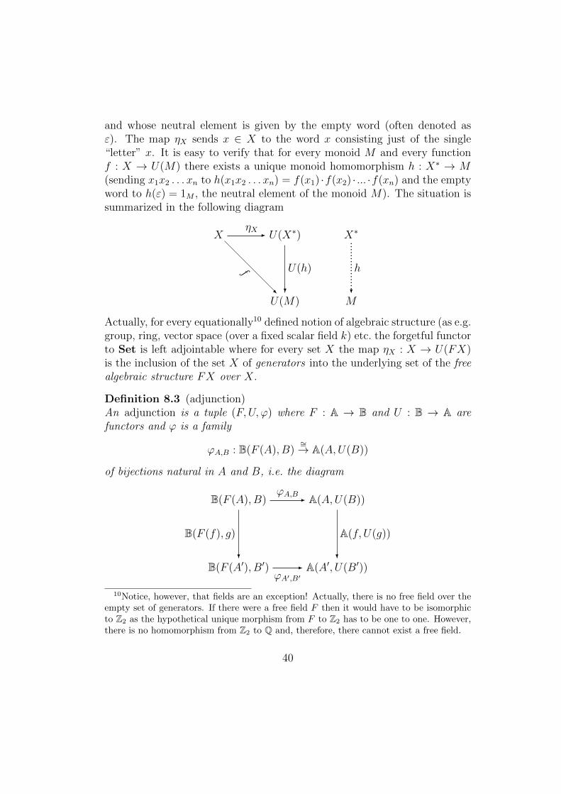
and whose neutral element is given by the empty word (often denoted asε). The map ηX sends x ∈ X to the word x consisting just of the single“letter” x. It is easy to verify that for every monoid M and every functionf : X → U(M) there exists a unique monoid homomorphism h : X∗ → M(sending x1x2 . . . xn to h(x1x2 . . . xn) = f(x1) ·f(x2) · ... ·f(xn) and the emptyword to h(ε) = 1M , the neutral element of the monoid M). The situation issummarized in the following diagram

XηX- U(X∗) X∗

U(M)

U(h)

?

f

-

M

h

?

.................

Actually, for every equationally10 defined notion of algebraic structure (as e.g.group, ring, vector space (over a fixed scalar field k) etc. the forgetful functorto Set is left adjointable where for every set X the map ηX : X → U(FX)is the inclusion of the set X of generators into the underlying set of the freealgebraic structure FX over X.

Definition 8.3 (adjunction)An adjunction is a tuple (F,U, ϕ) where F : A → B and U : B → A arefunctors and ϕ is a family

ϕA,B : B(F (A), B)∼=→ A(A,U(B))

of bijections natural in A and B, i.e. the diagram

B(F (A), B)ϕA,B- A(A,U(B))

B(F (A′), B′)

B(F (f), g)

?

ϕA′,B′- A(A′, U(B′))

A(f, U(g))

?

10Notice, however, that fields are an exception! Actually, there is no free field over theempty set of generators. If there were a free field F then it would have to be isomorphicto Z2 as the hypothetical unique morphism from F to Z2 has to be one to one. However,there is no homomorphism from Z2 to Q and, therefore, there cannot exist a free field.

40

commutes for all morphisms f : A′ → A in A and g : B → B′ in B.We write F a U iff there is a ϕ such that (F,U, ϕ) is an adjunction. ♦

Obviously, in the above definition the condition on ϕ can be formulatedmore concisely as the requirement that ϕ is a natural isomorphism fromB(F (−1),−2) to A(−1, U(−2)) in the functor category SetA

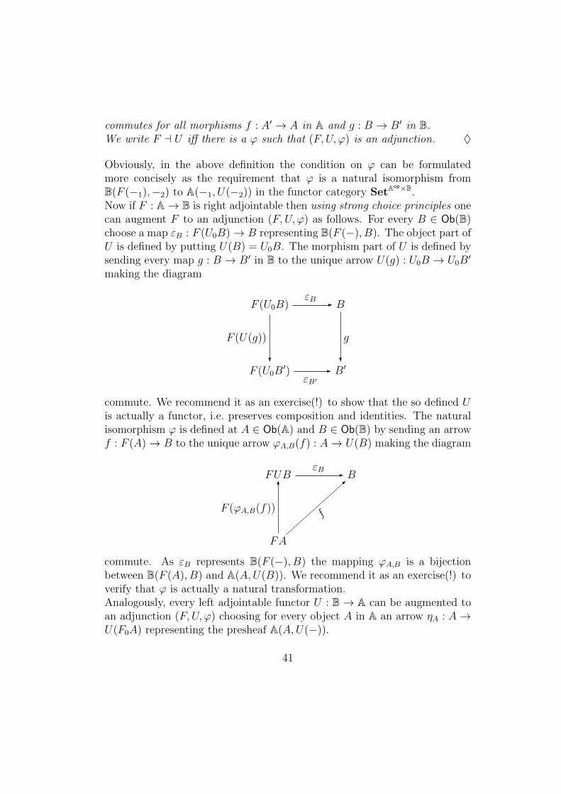
op×B.Now if F : A→ B is right adjointable then using strong choice principles onecan augment F to an adjunction (F,U, ϕ) as follows. For every B ∈ Ob(B)choose a map εB : F (U0B)→ B representing B(F (−), B). The object part ofU is defined by putting U(B) = U0B. The morphism part of U is defined bysending every map g : B → B′ in B to the unique arrow U(g) : U0B → U0B

′

making the diagram

F (U0B)εB - B

F (U0B′)

F (U(g))

?

εB′- B′

g

?

commute. We recommend it as an exercise(!) to show that the so defined Uis actually a functor, i.e. preserves composition and identities. The naturalisomorphism ϕ is defined at A ∈ Ob(A) and B ∈ Ob(B) by sending an arrowf : F (A)→ B to the unique arrow ϕA,B(f) : A→ U(B) making the diagram

FUBεB - B

FA

F (ϕA,B(f))

6

f

-

commute. As εB represents B(F (−), B) the mapping ϕA,B is a bijectionbetween B(F (A), B) and A(A,U(B)). We recommend it as an exercise(!) toverify that ϕ is actually a natural transformation.Analogously, every left adjointable functor U : B→ A can be augmented toan adjunction (F,U, ϕ) choosing for every object A in A an arrow ηA : A→U(F0A) representing the presheaf A(A,U(−)).

41

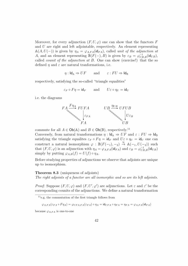
Moreover, for every adjunction (F,U, ϕ) one can show that the functors Fand U are right and left adjointable, respectively. An element representingA(A,U(−)) is given by ηA = ϕA,FA(idFA), called unit of the adjunction atA, and an element representing B(F (−), B) is given by εB = ϕ−1

UB,B(idUB),called counit of the adjunction at B. One can show (exercise!) that the sodefined η and ε are natural tranformations, i.e.

η : IdA ⇒ UF and ε : FU ⇒ IdB

respectively, satisfying the so-called “triangle equalities”

εF Fη = idF and Uε ηU = idU

i.e. the diagrams

FAFηA- FUFA UB

ηUB- UFUB

FA

εFA?

=========UB

UεB?

=========

commute for all A ∈ Ob(A) and B ∈ Ob(B), respectively.11

Conversely, from natural transformations η : IdA ⇒ UF and ε : FU ⇒ IdBsatisfying the triangle equalites εF Fη = idF and Uε ηU = idU one can

construct a natural isomorphism ϕ : B(F (−1),−2)∼=→ A(−1, U(−2)) such

that (F,U, ϕ) is an adjunction with ηA = ϕA,FA(idFA) and εB = ϕ−1UB,B(idUB)

simply by putting ϕA,B(f) = U(f) ηA.

Before studying properties of adjunctions we observe that adjoints are uniqueup to isomorphism.

Theorem 8.3 (uniqueness of adjoints)The right adjoints of a functor are all isomorphic and so are its left adjoints.

Proof: Suppose (F,U, ϕ) and (F,U ′, ϕ′) are adjunctions. Let ε and ε′ be thecorresponding counits of the adjunctions. We define a natural transformation

11e.g. the commutation of the first triangle follows from

ϕA,FA(εFA FηA) = ϕUFA,FA(εFA) ηA = idUFA ηFA = ηFA = ϕA,FA(idFA)

because ϕA,FA is one-to-one

42

ι : U ⇒ U ′ as follows: for B ∈ Ob(B) let ιB : U(B) → U ′(B) be the uniquearrow in A such that ε′B F (ιB) = εB. Notice that ιB is an isomorphismwhose inverse is given by the unique arrow ι−1

B satisfying εB F (ι−1B ) = ε′B.

That ι = (ιB)B∈Ob(B) is a natural transformation can be seen as follows.Suppose that g : B → B′ then we have

ε′B′ F (U ′(g) ιB) = ε′B′ FU ′g F (ιB) = g ε′B F (ιB) = g εB

and

ε′B′ F (ιB′ U(g)) = ε′B′ F (ιB′) FUg = εB′ FUg = g εB

and, therefore, also ε′B′ F (U ′(g) ιB) = ε′B′ F (ιB′ U(g)) from which itfollows that U ′(g) ιB = ιB′ U(g) as desired.Analogously, one proves that left adjoints of a functor are unique up toisomorphism.

Theorem 8.4 Right adjointable functors preserve colimits and left adjointablefunctors preserve limits.

Proof: We just prove the first claim as the second one follows by duality.Thus, suppose that F : A → B is right adjointable, i.e. for all B ∈ Ob(B)there is an arrow εB : FUB → B such that for all f : FA → B in B thereis a unique arrow g : A → UB in A such that εB Fg = f . Now supposeD : G→ A is a diagram in A with colimiting cocone µ : D ⇒ ∆(A). We willshow that

Fµ = (F (µI) : F (D(I))→ F (A))I∈G0

is a colimiting cocone for FD. First we show that Fµ is a cocone. Forthat purpose suppose u : I → J in G. Then we have FµJ F (D(u)) = FµIbecause µJD(u) = µI (as µ is a cocone overD) and F preserves composition.Thus, it remains to show that Fµ is a colimiting cocone for FD. For thatpurpose suppose τ : FD ⇒ ∆(X). For I ∈ G0 let σI : D(I) → UX be theunique arrow satisfying εX F (σI) = τI . We show that σ : D ⇒ ∆(UX).For u : I → J in G we have

εX F (σI) = τI = τJ F (D(u)) = εX F (σJ) F (D(u)) = εX F (σJD(u))

and, therefore, also σI = σJ D(u). Accordingly, there exists a unique arrowh : A→ UX with h µI = σI for all I ∈ G0. Thus, for all I ∈ G0 we have

εX Fh FµI = εX FσI = τI

43

from which it follows that k = εX Fh is a mediating arrow from Fµ to τ .We have to show that k is unique with this property. Suppose k′ : FA→ Xwith k′ FµI = τI for all I ∈ G0. Then there exists h′ : A → UX withεX Fh′ = k′. Then for all I ∈ G0 we have

εX F (h′µI) = εX Fh′ FµI = k′ FµI = τI = εX F (σI)

from which it follows that h′µI = σI for all I ∈ G0. Thus, we have h = h′ (asµ is a colimiting cocone) and, accordingly, also k = εX Fh = εX Fh′ = k′

as desired.

Next we characterise some properties of a functor under the assumption thatit has a right adjoint.

Theorem 8.5 Suppose F a U : B → A is an adjunction with unit η : Id ⇒UF . Then

(1) F is faithful iff all ηA are monic

(2) F is full iff all ηA are split epic, i.e. ηA s = id for some s : UFA→ A

(3) F is full and faithful iff η is a natural isomorphism.

Proof:ad (1) : For morphisms f1, f2 : A′ → A in A we have

ηA f1 = ηA f2 iff UFf1 ηA′ = UFf2 ηA′ iff Ff1 = Ff2

from which it follows that F is faithful iff all ηA are monic.ad (2) : If F is full then for all A ∈ Ob(A) there is a map sA : UFA → Awith F (sA) = εFA : FUFA → FA. Thus, we have idUFA = ϕ(εFA) =ϕ(idFA F (sA)) = ηA sA as desired.For the reverse direction suppose ηAsA = idUFA for all A ∈ Ob(A). Supposeg : FA′ → FA. We show that g = Ff for f = sA Ug ηA′ . As F a U it isequivalent to show that Ug ηA′ = UFf ηA′ which can be seen as follows

UFf ηA′ = ηA f = ηA sA Ug ηA′ = Ug ηA′

ad (3) : immediate from (1) and (2).

Actually, claim (3) of Theorem 8.5 can be strengthened as follows.

44

Lemma 8.1 If F a U : B → A and UF is isomorphic to IdA then η is anatural isomorphism, too.

Proof: Let ι : Id⇒ UF be a natural isomorphism. Then η is an isomorphismas for every A the arrow ηA is inverted by jA = ι−1

A UεFA UFιA which canbe seen as follows. We have

jA ηA = ι−1A UεFA UFιA ηA = ι−1

A UεFA ηUFA ιA = ι−1A ιA = idA

and from this it follows that

ι−1A ηA jA ιA = (naturality of η)

= ι−1A UFjA UFιA ηA = (naturality of ι−1)

= jA ιA ι−1A ηA =

= jA ηA = idA

and therefore ηA jA = ιA ι−1A = idUFA.

We leave it as an exercise(!) to formulate and verify the dual analogues ofTheorem 8.5 and Lemma 8.1.

45

9 Adjoint Functor Theorems

Already back in the 1960ies P.J.Freyd proved a couple of theorems provid-ing criteria for the existence of adjoints under fairly general assumptions.The exposition of Freyd’s Adjoint Functor Theorems given in this sectionessentially follows the presentation given in [ML].

We need the following two lemmas whose easy proof we leave as a straight-forward exercise(!) to the reader.

Lemma 9.1 Let C be a category with small limits and U : C→ B a functorpreserving small limits. Then for every object B in B the comma categoryB↓U has small limits.

Lemma 9.2 Let C be a locally small category and U : C → B a functor.Then for every object B in B the comma category B↓U is locally small, too.

The key idea of the general Adjoint Functor Theorem (FAFT) is to establishthe existence of a weakly initial object from which there follows the exis-tence of an initial object under the assumptions of local smallness and smallcompleteness.

Definition 9.1 An object W of a category C is called weakly initial iff forevery object A of C there exists a morphism from W to A. ♦

Lemma 9.3 Let C be a locally small category having all small limits. ThenC has an initial object if and only if C has a weakly initial object.

Proof: Obviously, every initial object in C is also weakly initial in C.Conversely, suppose that W is weakly initial in C. Let i : I W be anequaliser of all endomorphisms of W which exists because C(W,W ) is smalland C has all small limits. We show that I is initial in C. Let A be an objectin C. Then there exists a map f from W to A and thus f i : I → A. Foruniqueness suppose that f1, f2 : I → A. Let e : E I be an equaliser of f1

and f2. As W is weakly initial there exists a map p : W → E. As i equalisesall endomorphisms of W we have i = i e p i. As i is monic it follows thatidI = e p i. Thus, we have also e p i e = e from which it follows thatp i e = idE as e being an equaliser is monic. Thus e is an isomorphism(with inverse p i) from which it follows that f1 = f2 as desired.

46

Theorem 9.1 (General Adjoint Functor Theorem (FAFT)) Let C be a lo-cally small category with small limits. Then a functor U : C → B has a leftadjoint iff U preserves small limits and satisfies the following

Solution Set Condition For every object B of B there existsa small family (fi : B → U(Xi))i∈I such that for every mapg : B → U(X) for some i ∈ I there is a map h : Xi → X withg = U(h) fi.

Proof: Due to Theorem 8.4 a functor U preserves limits whenever it has aleft adjoint F . Moreover, for every B ∈ B the unit ηB : B → UFB of F a Uat B is initial in B↓U from which it follows that the solution set conditionholds.Suppose that U preserves small limits and the solution set condition holds.For U having a left adjoint it suffices to show that for every B ∈ B thecomma category B↓U has an initial object. This, however, follows fromLemma 9.3 because B↓U is locally small by Lemma 9.2, has all small limitsby Lemma 9.1 and the solution set condition gives rise to a weakly initialobject in B↓U by taking the product of the small family (fi)i∈I in B↓U .

Notice that the solution set condition is actually necessary as can be seenfrom the following counterexample. Let C = Ordop where Ord is the largeposet of (small) ordinals considered as a category. Let U be the uniquefunctor from C to the terminal category 1. Obviously, all assumptions ofTheorem 9.1 are satisfied with the exception of the solution set condition.Now if U had a left adjoint this would give rise to an initial object in C whichdoes not exist as there is no greatest (small) ordinal.Next we discuss a few applications of FAFT.First we show that for every category A of equationally defined algebras (andall homomorphisms between them) the forgetful functor U : A → Set hasa left adjoint F , i.e. that free A-algebras always exist. Every equationallydefined class A of algebras is locally small and has small limits which arepreserved by U . Thus, the assumptions of FAFT are satisfied. The solutionset condition is also valid for the following reason. Let I be a set. Then forevery A ∈ A every function f : I → A factors through the least subalgebraof A generated by the image of I under f . As up to isomorphism there isjust a small collection of algebras in A which are generated by a subset ofcardinality less or equal the cardinality of I there is up to isomorphism justa small collection of maps f : I → A such that A is the only subalgebra of A

47

containing the image of I under f . Thus, the forgetful functor U : A→ Sethas a left adjoint F .From universal algebra one knows that the map ηI sending elements of Ito the corresponding generators in U(F (I)) is one-to-one provided A con-tains algebras of arbitrarily big size. This can be shown also by the following“abstract nonsense” argument without any inspection of the actual construc-tion of the free algebra F (I). Suppose ηI(i) = ηI(j) for some i, j ∈ I withi 6= j. Let A be an algebra with A ≥ |I|. Then there exists a functionf : I → U(A) which is one-to-one. Thus, by adjointness there exists a ho-momorphism h : F (I) → A with f = U(h) ηI rendering ηI(i) = ηI(j)impossible because we have h(ηI(i)) = f(i) 6= f(j) = h(ηI(j)).Notice, however, that the forgetful functor from the category CBool of com-plete Boolean algebras to Set does not have a left adjoint because thereexist12 arbitrarily big complete Boolean algebras generated by a countablesubset. As CBool is locally small and has small limits preserved by theforgetful functor U this counterexample illustrates again the necessity of thesolution set condition.Next we consider the forgetful functor U from CompHaus to Set whereCompHaus is the full subcategory of Sp on compact Hausdorff spaces.FAFT is applicable because CompHaus is locally small and has small limitswhich are preserved by U . Let I be a set. Then every map f : I → U(X)factors through f [I], the closure of the image of X under f . Thus, forverifying the solution set condition it suffices to consider only maps f : I →U(X) with dense image. For any such map f the size of X is bounded bythe size of P2(I) for the following reason. Define e : X → P2(I) by sendingx ∈ X to the collection of all J ⊆ I with x ∈ f [J ]. For showing thate is one-to-one suppose x1 and x2 are distinct elements of X. Then thereexist open disjoint sets U1 and U2 with xi ∈ Ui for i = 1, 2 from which itfollows that f−1[U1] 6∈ e(x2) and f−1[U2] 6∈ e(x1). But for i = 1, 2 we havexi ∈ f [f−1[Ui]] since for every open neighbourhood V of xi the sets f [I] andUi ∩ V have non-empty intersection (as f [I] is dense in X by assumption).Thus f−1[Ui] ∈ e(xi) for i = 1, 2 and, therefore, since f−1[U1] 6∈ e(x2) andf−1[U2] 6∈ e(x1) it follows that e(x1) 6= e(x2) as desired. Up to isomorphismthere is just a small collection of compact Hausdorff spaces with cardinalityless or equal 22|I| . As CompHaus is locally small up to isomorphism there

12as has been shown in R. Solovay New proof of a theorem of Gaifman and HalesBull.Amer.Math.Soc.72, 1966, pp.282–284

48

is just a small collection of continuous maps in CompHaus that start fromI and have dense image. Thus, the solution set condition holds for U fromwhich it follows by FAFT that U has a left adjoint. By an even simplerargument it can be shown (exercise!) that the forgetful functor from Haus,the category of Hausdorff spaces and continuous maps, into Sp has a leftadjoint, i.e. that Haus forms a full reflective subcategory of Sp.

Next we prove the Special Adjoint Functor Theorem providing a criterionwhich is easier to check than the solution set condition but requires slightlystronger assumptions.

Definition 9.2 A family (Ci)i∈I of objects in a category C is called cogen-erating iff maps f, g : Y → X in C are equal whenever for all i ∈ I it holdsthat h f = h g for all h : X → Ci. ♦

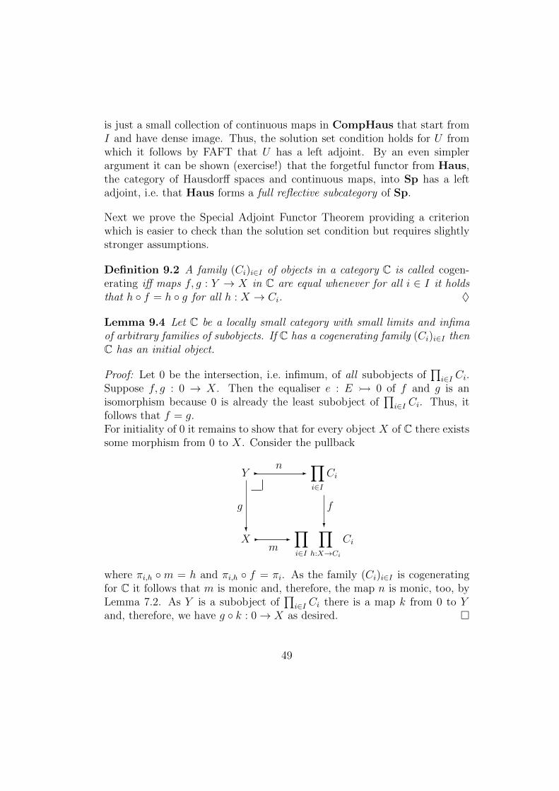
Lemma 9.4 Let C be a locally small category with small limits and infimaof arbitrary families of subobjects. If C has a cogenerating family (Ci)i∈I thenC has an initial object.

Proof: Let 0 be the intersection, i.e. infimum, of all subobjects of∏

i∈I Ci.Suppose f, g : 0 → X. Then the equaliser e : E 0 of f and g is anisomorphism because 0 is already the least subobject of

∏i∈I Ci. Thus, it

follows that f = g.For initiality of 0 it remains to show that for every object X of C there existssome morphism from 0 to X. Consider the pullback

Y-n

-∏i∈I

Ci

X

g

?-

m-∏i∈I

∏h:X→Ci

Ci

f

?

where πi,h m = h and πi,h f = πi. As the family (Ci)i∈I is cogeneratingfor C it follows that m is monic and, therefore, the map n is monic, too, byLemma 7.2. As Y is a subobject of

∏i∈I Ci there is a map k from 0 to Y

and, therefore, we have g k : 0→ X as desired.

49

Theorem 9.2 (Special Adjoint Functor Theorem (SAFT)) Let C be a locallysmall category with small limits, infima of arbitrary families of subobjects anda cogenerating family (Ci)i∈I . Then for locally small categories B a functorU : C → B has a left adjoint iff U preserves small limits and infima ofarbitrary families of subobjects.

Proof: Of course, if U has a left adjoint then it preserves all limits, i.e. inparticular small limits and arbitrary intersections of subobjects.For showing the reverse direction suppose that U preserves small limits andarbitrary intersections of subobjects. We will show that for all objects B ofB the comma category B↓U has an initial object from which it then followsthat U has a left adjoint. From Lemma 9.1 and 9.2 it follows that B↓Uis locally small and has small limits. As C has and U preserves arbitraryintersections of subobjects it follows that B↓U has arbitrary intersectionsof subobjects, too. As B is locally small the collection

⋃i∈I B(B,U(Ci)) is

small, too, and one easily shows that it provides a cogenerating family forB↓U . Thus, it follows by Lemma 9.4 that B↓U has an initial object.

In most examples the extra assumption of subobjects being closed underarbitrary intersections is redundant as in these cases the categories underconsideration are well-powered in the following sense.

Definition 9.3 A category C is well-powered iff for every object A of C theposet SubC(A) of subobjects of A is small. ♦

Obviously, if a category C is well-powered and has small limits then C hasalso arbitrary intersections of subobjects. Moreover, if U : C→ B preservessmall limits then U preserves13 also arbitrary intersections of subobjects.This gives rise to the following even more useful version of the Special AdjointFunctor Theorem (SAFT).

Theorem 9.3 Let C be a category which is locally small, well-powered andsmall complete. If C admits a small cogenerating family and U : C→ B withB locally small then U has a left adjoint iff U preserves small limits.

13From preservation of pullbacks it follows that monos are preserved, too.

50

Proof: The claim is immediate from Theorem 9.2 because if C is well-poweredand U preserves small limits then U preserves also arbitrary intersections ofsubobjects.

As an illustration of the power of SAFT we show that the inclusion U ofthe category CompHaus of compact Hausdorff spaces into the categorySp has a left adjoint β called Stone-Cech compactification. Obviously, bothCompHaus and Sp are locally small, have small limits and are well-powered.Due to Urysohn’s Separation Lemma continuous maps to the space [0, 1]separate points in compact Hausdorff spaces. Thus, by Theorem 9.3 theforgetful functor U has a left adjoint β. Unwinding the proof of SAFTone can see that for a space X its reflection14 to CompHaus is given byηX : X → β(X) where β(X) is the closure of the image of the map

ηX : X → X : x 7→ (f 7→ f(x))

with X =∏

f∈Sp(X,[0,1])[0, 1] (which is compact by Tychonoff’s Theorem).

14a left adjoint to a full and faithful functor is commonly called a reflection

51

10 Monads

Every adjunction F a U : B → A induces a so-called monad (T, η, µ) on Awhere T = UF : A → A, η : IdA → T is the unit of the adjunction andµ : T 2 → T is given by µA = UεFA. Using the triangular equalities for unitη and counit ε of the adjunction F a U it is a straightforward exercise(!) toshow that (T, η, µ) is a monad in the sense of the following definition.

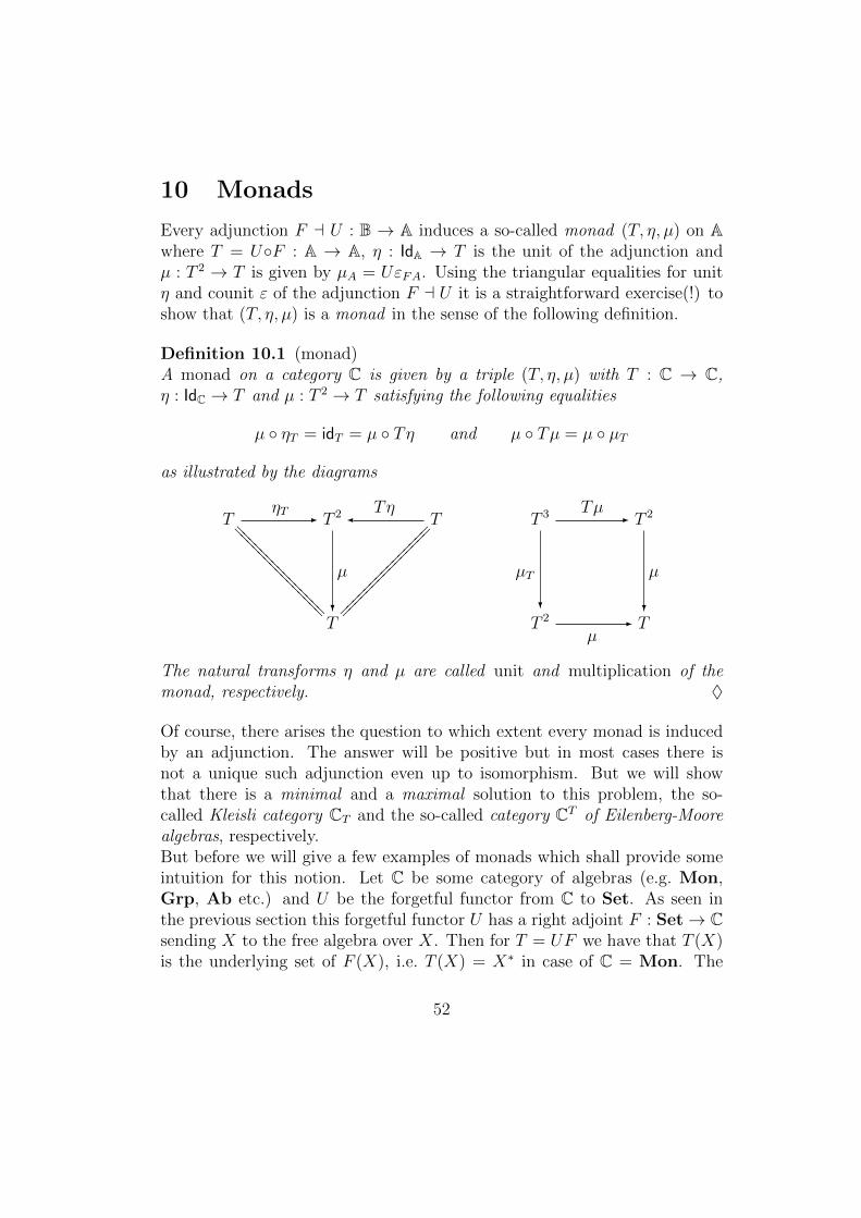
Definition 10.1 (monad)A monad on a category C is given by a triple (T, η, µ) with T : C → C,η : IdC → T and µ : T 2 → T satisfying the following equalities

µ ηT = idT = µ Tη and µ Tµ = µ µT

as illustrated by the diagrams

TηT - T 2

TηT T 3 Tµ

- T 2

T

µ

?====

====

====

===

===============T 2

µT

?

µ- T

µ

?

The natural transforms η and µ are called unit and multiplication of themonad, respectively. ♦

Of course, there arises the question to which extent every monad is inducedby an adjunction. The answer will be positive but in most cases there isnot a unique such adjunction even up to isomorphism. But we will showthat there is a minimal and a maximal solution to this problem, the so-called Kleisli category CT and the so-called category CT of Eilenberg-Moorealgebras, respectively.But before we will give a few examples of monads which shall provide someintuition for this notion. Let C be some category of algebras (e.g. Mon,Grp, Ab etc.) and U be the forgetful functor from C to Set. As seen inthe previous section this forgetful functor U has a right adjoint F : Set→ Csending X to the free algebra over X. Then for T = UF we have that T (X)is the underlying set of F (X), i.e. T (X) = X∗ in case of C = Mon. The

52

function ηX : X → T (X) inserts the generators into the generated algebra,i.e. in case C = Mon we have that ηX(x) is the single letter word consistingof the letter x. More complex is µX : T 2(X)→ T (X) sending a term t overT (X) to the term µX(t) over X by interpreting the generators occuring in tas elements of T (X). In case C = Mon the operation µ sends w1 . . . wk inX∗∗ with wi = xi,1 . . . xi,ni

to x1,1 . . . x1,n1 . . . xk,1 . . . xk,nkin X∗. Notice that

in computer science this operation is called “flattening” (of lists).Generally, in computer science monads play an important role because theyallow one to capture so-called “computational effects” as for example non-termination. Consider the functor L : Set → Set (called lifting) sending Xto L(X) = X+∗ where ∗ is a distinguished element (representing nonter-mination). For f : X → Y the map L(f) : L(X) → L(Y ) behaves on Xlike f and sends ∗ to ∗. Let ηX be the function including X into X+∗and µX : L2(X)→ L(X) be the function sending the “two different “∗’s” ofL2(X) to ∗ and elements of X to themselves. One readily checks that thisdefines a monad on Set for which we will see later on that it captures non-termination (because the Kleisli category SetL will turn out as isomorphicto the category of sets and partial functions).Slightly more refined examples of “computational monads” are the followingones.Fix a set R of so-called “responses” and let T : Set → Set be the functorsending X to T (X) = RRX

and f : X → Y to

T (f) = RRf

: φ 7→ (p 7→ φ(pf))

i.e. T (f) = λφ:RRX.λf :RY .φ(λx:X.p(f(x))) in the language of simply typed

λ-calulus as familiar from functional programming. The unit ηX : X → RRX

sends x ∈ X to the map ηX(x) : RX → R : p 7→ p(x) and the multiplicationµX is given by Rη

RX , i.e.

µX(Φ) = λp:RX .Φ(ηRX (p)) = λp:RX .Φ(λφ:RRX

.φ(p))

in λ-calculus notation. This monad is called “continuation monad” as a“computation” φ ∈ RRX

is thought of as a “generalised point of X” describedby its “response” φ(p) to an “observation” or “continuation” p. We leave itas an exercise(!) to show that the continuation monad is induced by theadjunction R(·) a (R(·))op : Setop → Set.Another example is the so-called state monad which is described as follows.Fix a set S of states and define T (X) = (X×S)S whose elements c are

53

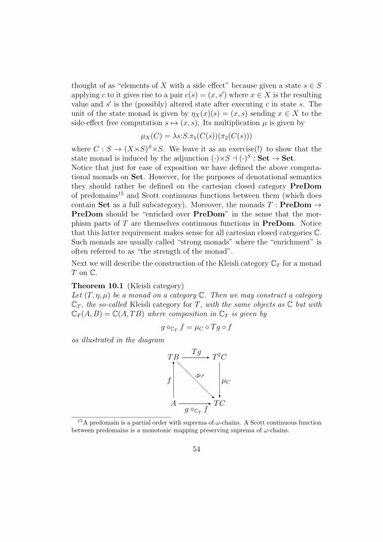
thought of as “elements of X with a side effect” because given a state s ∈ Sapplying c to it gives rise to a pair c(s) = (x, s′) where x ∈ X is the resultingvalue and s′ is the (possibly) altered state after executing c in state s. Theunit of the state monad is given by ηX(x)(s) = (x, s) sending x ∈ X to theside-effect free computation s 7→ (x, s). Its multiplication µ is given by

µX(C) = λs:S.π1(C(s))(π2(C(s)))

where C : S → (X×S)S×S. We leave it as an exercise(!) to show that thestate monad is induced by the adjunction (·)×S a (·)S : Set→ Set.Notice that just for ease of exposition we have defined the above computa-tional monads on Set. However, for the purposes of denotational semanticsthey should rather be defined on the cartesian closed category PreDomof predomains15 and Scott continuous functions between them (which doescontain Set as a full subcategory). Moreover, the monads T : PreDom →PreDom should be “enriched over PreDom” in the sense that the mor-phism parts of T are themselves continuous functions in PreDom. Noticethat this latter requirement makes sense for all cartesian closed categories C.Such monads are usually called “strong monads” where the “enrichment” isoften referred to as “the strength of the monad”.

Next we will describe the construction of the Kleisli category CT for a monadT on C.

Theorem 10.1 (Kleisli category)Let (T, η, µ) be a monad on a category C. Then we may construct a categoryCT , the so-called Kleisli category for T , with the same objects as C but withCT (A,B) = C(A, TB) where composition in CT is given by

g CTf = µC Tg f

as illustrated in the diagram

TBTg- T 2C

A

f

6

g CTf- TC

µC

?

g †

-

15A predomain is a partial order with suprema of ω-chains. A Scott continuous functionbetween predomains is a monotonic mapping preserving suprema of ω-chains.

54

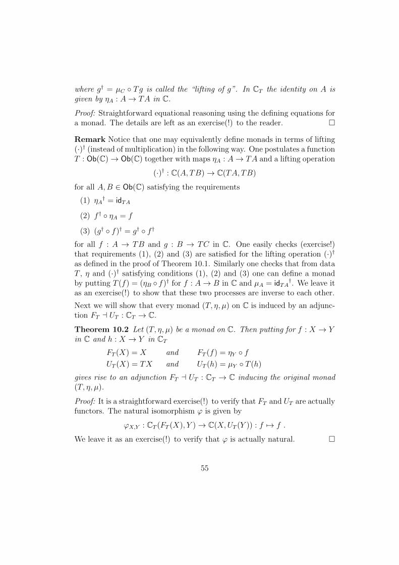
where g† = µC Tg is called the “lifting of g”. In CT the identity on A isgiven by ηA : A→ TA in C.

Proof: Straightforward equational reasoning using the defining equations fora monad. The details are left as an exercise(!) to the reader.

Remark Notice that one may equivalently define monads in terms of lifting(·)† (instead of multiplication) in the following way. One postulates a functionT : Ob(C)→ Ob(C) together with maps ηA : A→ TA and a lifting operation

(·)† : C(A, TB)→ C(TA, TB)

for all A,B ∈ Ob(C) satisfying the requirements

(1) ηA† = idTA

(2) f † ηA = f

(3) (g† f)† = g† f †

for all f : A → TB and g : B → TC in C. One easily checks (exercise!)that requirements (1), (2) and (3) are satisfied for the lifting operation (·)†as defined in the proof of Theorem 10.1. Similarly one checks that from dataT , η and (·)† satisfying conditions (1), (2) and (3) one can define a monadby putting T (f) = (ηB f)† for f : A→ B in C and µA = idTA

†. We leave itas an exercise(!) to show that these two processes are inverse to each other.

Next we will show that every monad (T, η, µ) on C is induced by an adjunc-tion FT a UT : CT → C.

Theorem 10.2 Let (T, η, µ) be a monad on C. Then putting for f : X → Yin C and h : X → Y in CT

FT (X) = X and FT (f) = ηY fUT (X) = TX and UT (h) = µY T (h)

gives rise to an adjunction FT a UT : CT → C inducing the original monad(T, η, µ).

Proof: It is a straightforward exercise(!) to verify that FT and UT are actuallyfunctors. The natural isomorphism ϕ is given by

ϕX,Y : CT (FT (X), Y )→ C(X,UT (Y )) : f 7→ f .

We leave it as an exercise(!) to verify that ϕ is actually natural.

55

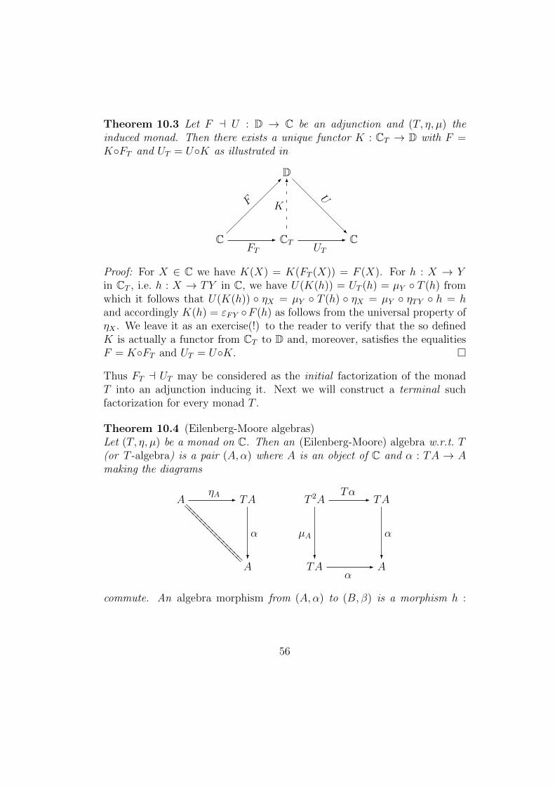
Theorem 10.3 Let F a U : D → C be an adjunction and (T, η, µ) theinduced monad. Then there exists a unique functor K : CT → D with F =KFT and UT = UK as illustrated in

D

CFT

-

F

-

CT

K

6

UT- C

U

-

Proof: For X ∈ C we have K(X) = K(FT (X)) = F (X). For h : X → Yin CT , i.e. h : X → TY in C, we have U(K(h)) = UT (h) = µY T (h) fromwhich it follows that U(K(h)) ηX = µY T (h) ηX = µY ηTY h = hand accordingly K(h) = εFY F (h) as follows from the universal property ofηX . We leave it as an exercise(!) to the reader to verify that the so definedK is actually a functor from CT to D and, moreover, satisfies the equalitiesF = KFT and UT = UK.

Thus FT a UT may be considered as the initial factorization of the monadT into an adjunction inducing it. Next we will construct a terminal suchfactorization for every monad T .

Theorem 10.4 (Eilenberg-Moore algebras)Let (T, η, µ) be a monad on C. Then an (Eilenberg-Moore) algebra w.r.t. T(or T -algebra) is a pair (A,α) where A is an object of C and α : TA → Amaking the diagrams

AηA - TA T 2A

Tα- TA

A

α

?

===============TA

µA

?

α- A

α

?

commute. An algebra morphism from (A,α) to (B, β) is a morphism h :

56

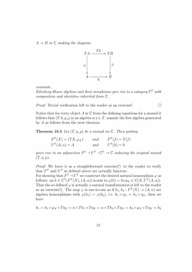
A→ B in C making the diagram

TATh

- TB

A

α

?

h- B

β

?

commute.Eilenberg-Moore algebras and their morphisms give rise to a category CT withcomposition and identities inherited from C.

Proof: Trivial verification left to the reader as an exercise!.

Notice that for every object A in C from the defining equations for a monad itfollows that (TA, µA) is an algebra w.r.t. T , namely the free algebra generatedby A as follows from the next theorem.

Theorem 10.5 Let (T, η, µ) be a monad on C. Then putting

F T (X) = (TX, µX) and F T (f) = T (f)

UT (A,α) = A and UT (h) = h

gives rise to an adjunction F T a UT : CT → C inducing the original monad(T, η, µ).

Proof: We leave it as a straightforward exercise(!) to the reader to verifythat F T and UT as defined above are actually functors.For showing that F T a UT we construct the desired natural isomorphism ϕ asfollows: an h ∈ CT (F T (X), (A,α)) is sent to ϕ(h) = hηX ∈ C(X,UT (A,α)).That the so defined ϕ is actually a natural transformation is left to the readeras an exercise(!). The map ϕ is one-to-one as if h1, h2 : F T (X)→ (A,α) arealgebra homorphisms with ϕ(h1) = ϕ(h2), i.e. h1 ηX = h2 ηX , then wehave

h1 = h1 µX TηX = α Th1 TηX = α Th2 TηX = h2 µX TηX = h2

57

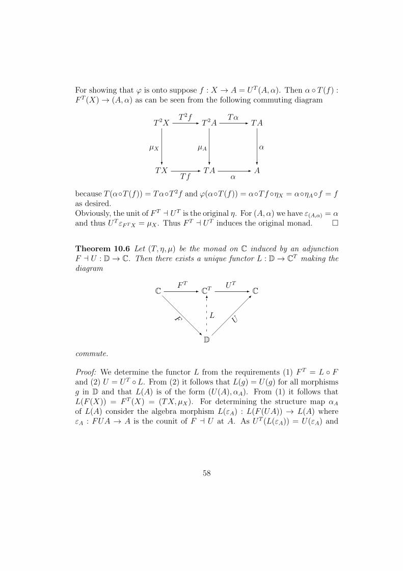
For showing that ϕ is onto suppose f : X → A = UT (A,α). Then α T (f) :F T (X)→ (A,α) as can be seen from the following commuting diagram

T 2XT 2f

- T 2ATα

- TA

TX

µX

?

Tf- TA

µA

?

α- A

α

?

because T (αT (f)) = TαT 2f and ϕ(αT (f)) = αTf ηX = αηAf = fas desired.Obviously, the unit of F T a UT is the original η. For (A,α) we have ε(A,α) = αand thus UT εFTX = µX . Thus F T a UT induces the original monad.

Theorem 10.6 Let (T, η, µ) be the monad on C induced by an adjunctionF a U : D→ C. Then there exists a unique functor L : D→ CT making thediagram

CF T

- CT UT- C

D

L

6

U

-

F

-

commute.

Proof: We determine the functor L from the requirements (1) F T = L Fand (2) U = UT L. From (2) it follows that L(g) = U(g) for all morphismsg in D and that L(A) is of the form (U(A), αA). From (1) it follows thatL(F (X)) = F T (X) = (TX, µX). For determining the structure map αAof L(A) consider the algebra morphism L(εA) : L(F (UA)) → L(A) whereεA : FUA → A is the counit of F a U at A. As UT (L(εA)) = U(εA) and

58

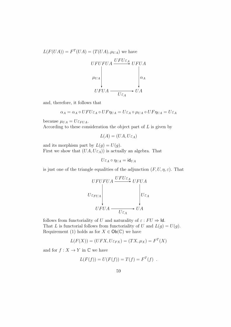
L(F (UA)) = F T (UA) = (T (UA), µUA) we have

UFUFUAUFUεA- UFUA

UFUA

µUA

?

UεA- UA

αA

?

and, therefore, it follows that

αA = αA UFUεA UFηUA = UεA µUA UFηUA = UεA

because µUA = UεFUA.According to these consideration the object part of L is given by

L(A) = (UA,UεA)

and its morphism part by L(g) = U(g).First we show that (UA,UεA)) is actually an algebra. That

UεA ηUA = idUA

is just one of the triangle equalities of the adjunction (F,U, η, ε). That

UFUFUAUFUεA- UFUA

UFUA

UεFUA

?

UεA- UA

UεA

?

follows from functoriality of U and naturality of ε : FU ⇒ Id.That L is functorial follows from functoriality of U and L(g) = U(g).Requirement (1) holds as for X ∈ Ob(C) we have

L(F (X)) = (UFX,UεFX) = (TX, µX) = F T (X)

and for f : X → Y in C we have

L(F (f)) = U(F (f)) = T (f) = F T (f) .

59

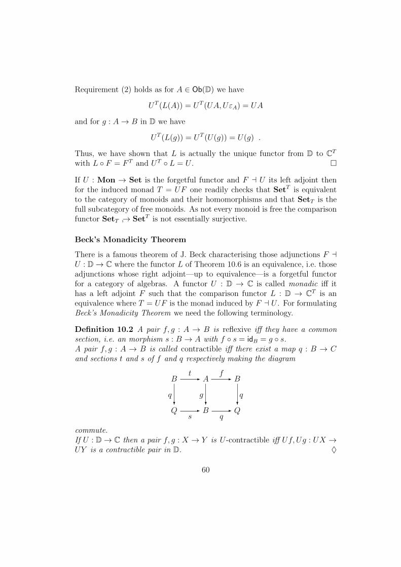
Requirement (2) holds as for A ∈ Ob(D) we have

UT (L(A)) = UT (UA,UεA) = UA

and for g : A→ B in D we have

UT (L(g)) = UT (U(g)) = U(g) .

Thus, we have shown that L is actually the unique functor from D to CT

with L F = F T and UT L = U .

If U : Mon → Set is the forgetful functor and F a U its left adjoint thenfor the induced monad T = UF one readily checks that SetT is equivalentto the category of monoids and their homomorphisms and that SetT is thefull subcategory of free monoids. As not every monoid is free the comparisonfunctor SetT → SetT is not essentially surjective.

Beck’s Monadicity Theorem

There is a famous theorem of J. Beck characterising those adjunctions F aU : D→ C where the functor L of Theorem 10.6 is an equivalence, i.e. thoseadjunctions whose right adjoint—up to equivalence—is a forgetful functorfor a category of algebras. A functor U : D → C is called monadic iff ithas a left adjoint F such that the comparison functor L : D → CT is anequivalence where T = UF is the monad induced by F a U . For formulatingBeck’s Monadicity Theorem we need the following terminology.

Definition 10.2 A pair f, g : A → B is reflexive iff they have a commonsection, i.e. an morphism s : B → A with f s = idB = g s.A pair f, g : A → B is called contractible iff there exist a map q : B → Cand sections t and s of f and q respectively making the diagram

Bt- A

f- B

Q

q?

s- B

g?

q- Q

q?

commute.If U : D→ C then a pair f, g : X → Y is U -contractible iff Uf, Ug : UX →UY is a contractible pair in D. ♦

60

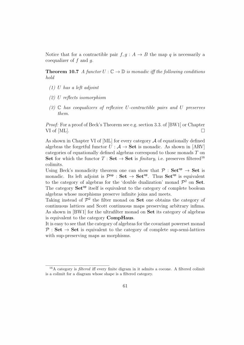
Notice that for a contractible pair f, g : A → B the map q is necessarily acoequalizer of f and g.

Theorem 10.7 A functor U : C→ D is monadic iff the following conditionshold

(1) U has a left adjoint

(2) U reflects isomorphism

(3) C has coequalizers of reflexive U-contractible pairs and U preservesthem.

Proof: For a proof of Beck’s Theorem see e.g. section 3.3. of [BW1] or ChapterVI of [ML].

As shown in Chapter VI of [ML] for every category A of equationally definedalgebras the forgetful functor U : A → Set is monadic. As shown in [ARV]categories of equationally defined algebras correspond to those monads T onSet for which the functor T : Set → Set is finitary, i.e. preserves filtered16

colimits.Using Beck’s monadicity theorem one can show that P : Setop → Set ismonadic. Its left adjoint is Pop : Set → Setop. Thus Setop is equivalentto the category of algebras for the ‘double dualization’ monad P2 on Set.The category Setop itself is equivalent to the category of complete booleanalgebras whose morphisms preserve infinite joins and meets.Taking instead of P2 the filter monad on Set one obtains the category ofcontinuous lattices and Scott continuous maps preserving arbitrary infima.As shown in [BW1] for the ultrafilter monad on Set its category of algebrasis equivalent to the category CompHaus.It is easy to see that the category of algebras for the covariant powerset monadP : Set → Set is equivalent to the category of complete sup-semi-latticeswith sup-preserving maps as morphisms.

16A category is filtered iff every finite digram in it admits a cocone. A filtered colimitis a colimit for a diagram whose shape is a filtered category.

61

Part II CATEGORICAL LOGIC

62

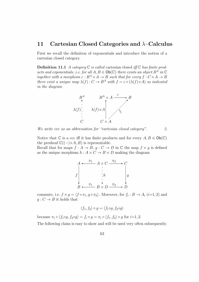
11 Cartesian Closed Categories and λ–Calculus

First we recall the definition of exponentials and introduce the notion of acartesian closed category.

Definition 11.1 A category C is called cartesian closed iff C has finite prod-ucts and exponentials, i.e. for all A,B ∈ Ob(C) there exists an object BA in Ctogether with a morphism ε : BA×A→ B such that for every f : C×A→ Bthere exist a unique map λ(f) : C → BA with f = ε (λ(f)×A) as indicatedin the diagram

BA BA × Aε- B

C

λ(f)

6

C × A

λ(f)×A

6

f

-

We write ccc as an abbreviation for “cartesian closed category”. ♦

Notice that C is a ccc iff it has finite products and for every A,B ∈ Ob(C)the presheaf C((−)×A,B) is representable.Recall that for maps f : A → B, g : C → D in C the map f × g is definedas the unique morphism h : A× C → B ×D making the diagram

A π1

A× Cπ2 - C

B

f

?

π1B ×D

h

? π2 - D

g

?

commute, i.e. f × g = 〈f π1, g π2〉. Moreover, for fi : B → Ai (i=1, 2) andg : C → B it holds that

〈f1, f2〉 g = 〈f1g, f2g〉

because πi 〈f1g, f2g〉 = fi g = πi 〈f1, f2〉 g for i=1, 2.

The following claim is easy to show and will be used very often subsequently.

63

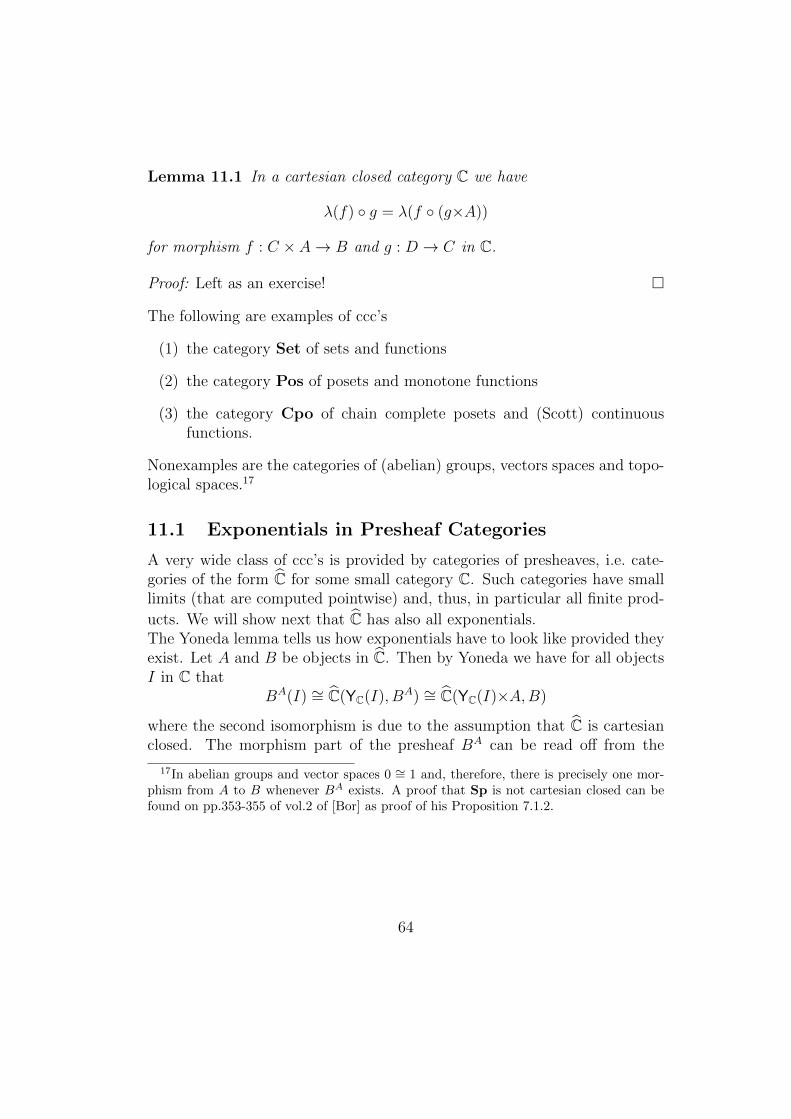
Lemma 11.1 In a cartesian closed category C we have

λ(f) g = λ(f (g×A))

for morphism f : C × A→ B and g : D → C in C.

Proof: Left as an exercise!

The following are examples of ccc’s

(1) the category Set of sets and functions

(2) the category Pos of posets and monotone functions

(3) the category Cpo of chain complete posets and (Scott) continuousfunctions.

Nonexamples are the categories of (abelian) groups, vectors spaces and topo-logical spaces.17

11.1 Exponentials in Presheaf Categories

A very wide class of ccc’s is provided by categories of presheaves, i.e. cate-gories of the form C for some small category C. Such categories have smalllimits (that are computed pointwise) and, thus, in particular all finite prod-

ucts. We will show next that C has also all exponentials.The Yoneda lemma tells us how exponentials have to look like provided theyexist. Let A and B be objects in C. Then by Yoneda we have for all objectsI in C that

BA(I) ∼= C(YC(I), BA) ∼= C(YC(I)×A,B)

where the second isomorphism is due to the assumption that C is cartesianclosed. The morphism part of the presheaf BA can be read off from the

17In abelian groups and vector spaces 0 ∼= 1 and, therefore, there is precisely one mor-phism from A to B whenever BA exists. A proof that Sp is not cartesian closed can befound on pp.353-355 of vol.2 of [Bor] as proof of his Proposition 7.1.2.

64

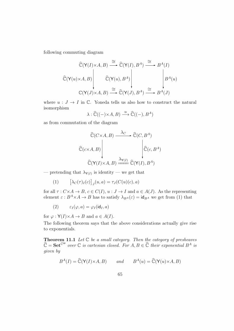
following commuting diagram

C(Y(I)×A,B)∼=- C(Y(I), BA)

∼=- BA(I)

C(Y(J)×A,B)

C(Y(u)×A,B)

? ∼=- C(Y(J), BA)

C(Y(u), BA)

? ∼=- BA(J)

BA(u)

?

where u : J → I in C. Yoneda tells us also how to construct the naturalisomorphism

λ : C((−)×A,B)∼=−→ C((−), BA)

as from commutation of the diagram

C(C×A,B)λC - C(C,BA)

C(Y(I)×A,B)

C(c×A,B)

?

====λY(I)

C(Y(I), BA)

C(c, BA)

?

— pretending that λY(I) is identity — we get that

(1)[λC(τ)I(c)

]J(u, a) = τJ(C(u)(c), a)

for all τ : C×A→ B, c ∈ C(I), u : J → I and a ∈ A(J). As the representingelement ε : BA×A→ B has to satisfy λBA(ε) = idBA we get from (1) that

(2) εI(ϕ, a) = ϕI(idI , a)

for ϕ : Y(I)×A→ B and a ∈ A(I).

The following theorem says that the above considerations actually give riseto exponentials.

Theorem 11.1 Let C be a small category. Then the category of presheavesC = SetC

op

over C is cartesian closed. For A,B ∈ C their exponential BA isgiven by

BA(I) = C(Y(I)×A,B) and BA(u) = C(Y(u)×A,B)

65

for I ∈ Ob(C) and u : J → I in C. The counit ε : BA×A → B (also calledevaluation map) is given by

εI(ϕ, a) = ϕI(idI , a)

for ϕ ∈ BA(I) and a ∈ A(I). For τ : C×A → B its exponential transposeλ(τ) : C → BA is given by[

λ(τ)I(c)]J(u, a) = τJ(C(u)(c), a)

for c ∈ C(I), u : J → I in C and a ∈ A(J).

Proof: It is an easy exercise (left to the reader) to check naturality of ε andλ(τ) as defined above. It remains to verify that

(β) ε (λ(τ)×A) = τ for all τ : C×A→ B and

(η) λ(ε (σ×A)) = σ for all σ : C → BA

i.e. that ε ((−)×A) is a natural bijection inverse to λ as desired.Condition (β) holds since[

ε (λ(τ)×A)]I(c, a) = εI(λ(τ)I(c), a)) =

= λ(τ)I(c)(idI , a) =

= τI(C(idI)(c), a) =

= τI(c, a)

and condition (η) holds since we have

λ(ε (σ×A))I(c)(u, a) = (ε (σ×A))J(C(u)(c), a) =

= εJ(σJ(C(u)(c)), a) =

= σJ(C(u)(c))(idJ , a) = (naturality of σ)

= BA(u)(σI(c))(idJ , a) =

=[σI(c)

]J(Y(u)(idJ), a) =

= σI(c)(u, a)

66

where u : J → I.

Admittedly, the construction of exponentials in presheaf categories may ap-pear as somewhat complicated at least at first sight. However, they tend tolook much nicer in particular cases like the following ones.

(1) Suppose C is a group, i.e. a category G with a single object ∗ all whose

morphisms are isomorphisms. Then for objects A and B in G according tothe general construction above the underlying set BA(∗) of the exponentialBA consists of all natural transformations τ : Y(∗)×A→ B. Obviously, sucha τ is uniquely determined by the map t : A(∗)→ B(∗) : a 7→ τ(1, a) wherewe write 1 for id∗ because by naturality of τ we have

τ(g, a) = τ(g, A(g)(A(g−1)(a))) = B(g)(τ(1, A(g−1)(a))) = B(g)(t(A(g−1)(a)))

i.e. τ(g,−) = B(g)tA(g−1). Moreover, one easily checks that for arbitraryfunctions t : A(∗) → B(∗) there is a unique natural transformation τ withτ(1, a) = t(a), namely τ(g, a) = B(g)(t(A(g−1)(a))).18 Thus, the exponential

BA in G is isomorphic to the set B(∗)A(∗) on which G acts by sending t ∈B(∗)A(∗) to BA(g)(t) = B(g) t A(g−1) for g in G.19

It is an instructive exercise(!) to explicitate how the global elements 1→ BA

correspond to the morphisms from A to B in G.

18We have to show that

B(h)(τ(g, a)) = τ(Y(∗)(h)(g), A(h)(a))

for which purpose we explicitate both sides of the equation. For the left hand side we have

B(h)(τ(g, a)) = (B(h) B(g) t A(g−1))(a)

and for the right hand side we have

τ(Y(∗)(h)(g), A(h)(a)) = τ(gh,A(h)(a)) = (B(gh) t A((gh)−1))(A(h)(a)) == (B(gh) t A(h−1g−1))(A(h)(a)) == (B(gh) t A(g−1) A(h−1)) A(h))(a) =

= (B(h) B(g) t A(g−1))(a)

and thus both sides of the equation are actually equal as desired.19This action is actually contravariant as

BA(gh)(t) = B(gh)tA(h−1g−1) = B(h)B(g)tA(g−1)A(h−1) = (BA(h)BA(g))(t)

due to the contravariance of A and B.

67

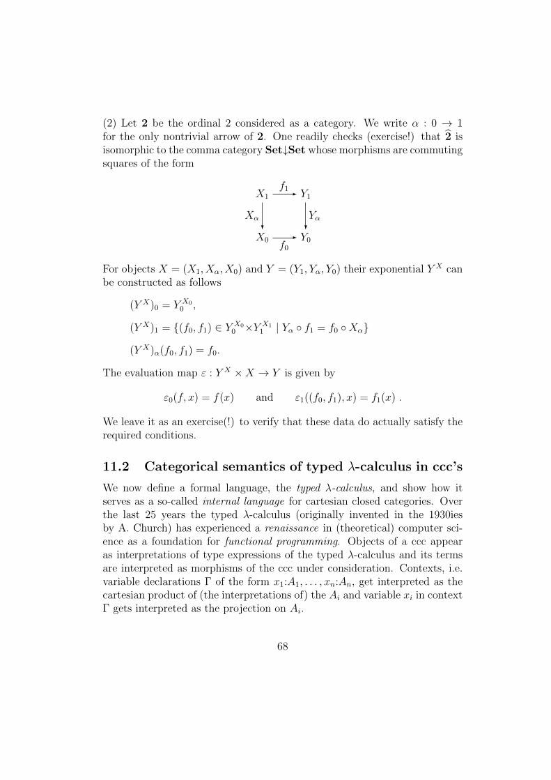
(2) Let 2 be the ordinal 2 considered as a category. We write α : 0 → 1for the only nontrivial arrow of 2. One readily checks (exercise!) that 2 isisomorphic to the comma category Set↓Set whose morphisms are commutingsquares of the form

X1

f1- Y1

X0

Xα?

f0

- Y0

Yα?

For objects X = (X1, Xα, X0) and Y = (Y1, Yα, Y0) their exponential Y X canbe constructed as follows

(Y X)0 = Y X00 ,

(Y X)1 = (f0, f1) ∈ Y X00 ×Y X1

1 | Yα f1 = f0 Xα

(Y X)α(f0, f1) = f0.

The evaluation map ε : Y X ×X → Y is given by

ε0(f, x) = f(x) and ε1((f0, f1), x) = f1(x) .

We leave it as an exercise(!) to verify that these data do actually satisfy therequired conditions.

11.2 Categorical semantics of typed λ-calculus in ccc’s

We now define a formal language, the typed λ-calculus, and show how itserves as a so-called internal language for cartesian closed categories. Overthe last 25 years the typed λ-calculus (originally invented in the 1930iesby A. Church) has experienced a renaissance in (theoretical) computer sci-ence as a foundation for functional programming. Objects of a ccc appearas interpretations of type expressions of the typed λ-calculus and its termsare interpreted as morphisms of the ccc under consideration. Contexts, i.e.variable declarations Γ of the form x1:A1, . . . , xn:An, get interpreted as thecartesian product of (the interpretations of) the Ai and variable xi in contextΓ gets interpreted as the projection on Ai.

68

But before describing the interpretation of typed λ-calculus in ccc’s we care-fully define its syntax.The types (or type expressions) of simply typed λ–calculus are defined in-ductively from a collection of base types via the following rules

• every base type is a type

• if A and B are types then A→B is a type.

These are the type expressions of traditional typed λ-calculus. For the pur-poses of an interpretation in cartesian closed categories, i.e. from a semanticalpoint of view, it turns out as convenient to close types under the followingtwo additional rules

• 1 is a type (also called unit type)

• if A and B are types then A×B is a type.

Contexts are expressions of the form

x1:A1, . . . , xn:An

where A1, . . . , An are type expressions and x1, . . . , xn is a list of pairwisedistinct variables. The purpose of a context x1:A1, . . . , xn:An is to declarethe variables x1, . . . , xn together with their types A1, . . . , An. We use captialGreek letters Γ,∆, . . . as (meta)variables ranging over contexts.Let C be a cartesian closed category. For interpreting the type expressionsin C we first fix an assignment of [[B]] ∈ Ob(C) for bases types B which isextended to arbitrary type expressions via the following inductive clauses

• [[A→B]] = [[A]]→ [[B]]

• [[A×B]] = [[A]]× [[B]]

• [[1]] = 1C

where X→Y stands for the exponential Y X in C and 1C is a chosen terminalobject in C. Contexts are interpreted as cartesian products, i.e.

[[x1 : A1, . . . , xn : An]] = [[A1]]× · · · × [[An]]

69

Next we will define the terms of typed λ-calculus. Terms not only have atype but are also defined relative to contexts in which their free variables aredeclared. We write

Γ ` t : A

for the judgement that t is a term of type A in context Γ. Traditionally, onewould call already t a term but, actually, one needs context Γ to determinethe meaning of t (as we shall see the type A of t will be determined uniquelyby t and Γ). The interpretation of Γ ` t : A will be a morphism from [[Γ]] to[[A]] in C, i.e.

[[Γ ` t : A]] : [[Γ]]→ [[A]]

and will be defined by structural recursion over terms. We will now intro-duce the various term formation rules together with the clauses fixing theinterpretation of the constructed terms.First of all variables declared in the context are terms, i.e.

(Var)x1 : A1, . . . , xn : An ` xi : Ai

which is interpreted as

πi : [[x1 : A1, . . . , xn : An]] −→ [[Ai]]

i.e. projection on the i-th component.Explicit definition of functions is provided by the rule

Γ, x : A ` t : B(λ)

Γ ` λx:A.t : A→B

where[[Γ ` λx:A.t : A→B]] = λ([[Γ, x : A ` t : B]])

i.e. ε ([[Γ ` λx:A.t : A→B]]× [[A]]) = [[Γ, x : A ` t : B]].Application of functions to arguments is provided by the rule

Γ ` t : A→B Γ ` s : A(App)

Γ ` t(s) : B

where the resulting term is interpreted as

[[Γ ` t(s)]] = ε 〈[[Γ ` t]], [[Γ ` s]]〉

70

Notice that we have written Γ ` t and Γ ` s instead of Γ ` t : A→B andΓ ` s, respectively, which is justified by the fact that for derivable judgementsΓ ` s : A the type A is determined uniquely simply because for each termformer there is precisely one introduction rule.This pleasant feature will be preserved by the remaining rules which weintroduce next.The following rule allows one to construct pairs

Γ ` t : A Γ ` s : B(Pair)

Γ ` 〈t, s〉 : A×B

where the constructed term will be interpreted as

[[Γ ` 〈t, s〉 : A×B]] = 〈[[Γ ` t : A]], [[Γ ` s : B]]〉

The following two rules (for i=1, 2)

Γ ` t : A1×A2(Proji)

Γ ` πi(t) : Ai

allow one to select components of pairs. Terms constructed by these ruleswill be interpreted as

[[Γ ` πi(t) : Ai]] = πi [[Γ ` t : A1×A2]]

with πi : [[A1]]×[[A2]]→ [[Ai]] the respective projection maps in C.The unique element of 1 may be constructed by the rule

(Unit)Γ ` ∗ : 1

where [[Γ ` ∗ : 1]] = ![[Γ]], the unique morphism from [[Γ]] to 1C in C.Up to now we have not considered equality between terms which we will donext. However, for this purpose we need a notion of substitution which onthe semantical level will be interpreted as composition of morphisms in C.Let Γ ≡ x1 : A1, . . . , xn : An and ∆ be contexts. A substitution σ : ∆ → Γis an n-tuple σ = 〈t1, . . . , tn〉 such that ∆ ` ti : Ai for i=1, . . . , n whoseinterpretation in C is given by

[[σ]] = 〈[[∆ ` t1]], . . . , [[∆ ` tn]]〉 : [[∆]]→ [[Γ]] .

71

Now for Γ ` t : A applying substitution σ : ∆→ Γ to it gives rise to a term∆ ` t[σ] : A whose interpretation is given by

[[∆ ` t[σ] : A]] = [[Γ ` t : A]] [[σ : ∆→ Γ]]

and which can be obtained syntactically by replacing (simultaneously) everyfree occurrence of xi by ti, i.e.

t[σ] ≡ t[t1, . . . , tn/x1, . . . , xn]

for which we often employ the more readable notation t[~t/~x], where, of course,one has to rename bound variables of t in such a way that substituting ti for xiin t does not bind free variables of ti, i.e. we employ capture-free substitutionas it is commonly called.That capture-free substitution actually amounts to composition on the se-mantical level is the contents of the following lemma.

Lemma 11.2 (Substitution Lemma)Whenever Γ ` t : A and σ : ∆→ Γ then

[[∆ ` t[σ] : A]] = [[Γ ` t : A]] [[σ]] .

Proof: We first show the claim for variable substitutions υ = 〈~t〉 where allti are variables declared in ∆. Obviously, such variable substitutions areinterpreted as target tuplings of projections.We proceed by induction on derivations of Γ ` t : A. All cases are trivialwith exception of the rule (λ) for which we exhibit the argument. Supposeas induction hypothesis that for sequent Γ, x:A ` t : B it holds that [[∆ `t[υ] : B]] = [[Γ, x:A ` t : A]] [[υ]] for all variable substitutions υ : ∆→ Γ, x:A.Let υ ≡ 〈v1, . . . , vn〉 : ∆→ Γ be a variable substitution. Then we have

[[Γ ` λx:A.t]] [[υ]] = λ([[Γ, x:A ` t]]) [[υ]] =

= λ([[Γ, x:A ` t]] ([[υ]]×id[[A]])) =

= λ([[Γ, x:A ` t]] [[〈v1, . . . , vn, x〉]]) = (ind.hyp.)

= λ([[∆, x:A ` t[~v, x/~x, x]]]) =

= [[∆ ` λx:A.t[~v/~x]]] =

= [[∆ ` λx:A.t[υ]]]

72

where 〈v1, . . . , vn, x〉 : ∆, x : A→ Γ, x : A is again a variable substitution.Now we prove the claim for general substitutions σ : ∆ → Γ. Again weproceed by induction on derivations of Γ ` t : A. Again all cases are trivialwith exception of the rule (λ) for which we exhibit the argument. Supposeas induction hypothesis that for sequent Γ, x:A ` t : B it holds that [[∆ `t[σ] : B]] = [[Γ, x:A ` t : A]] [[σ]] for all substitutions σ : ∆ → Γ, x:A. Nowsuppose τ ≡ 〈t1, . . . , tn〉 : ∆→ Γ. Then we have

[[Γ ` λx:A.t]] [[τ ]] = λ([[Γ, x:A ` t]]) [[τ ]] =

= λ([[Γ, x:A ` t]] ([[τ ]]×id[[A]])) = (*)

= λ([[Γ, x:A ` t]] [[〈t1, . . . , tn, x〉]]) = (ind.hyp.)

= λ([[∆, x:A ` t[~t, x/~x, x]]]) =

= [[∆ ` λx:A.t[~t/~x]]] =

= [[∆ ` λx:A.t[τ ]]]

where 〈t1, . . . , tn, x〉 : ∆, x : A → Γ, x : A. Notice that in (∗) we have usedthat [[∆, x : A ` ti]] = [[∆ ` ti]] π where π : [[∆]]× [[A]]→ [[∆]] as ensured bythe already established claim for variable substitutions.

Next we will show that the (β) and (η) rule (as defined below in Theo-rem 11.2) of typed λ-calculus are valid under interpretations in arbitrarycartesian closed categories. For this purpose consider an arbitrary, but fixedccc C together with an arbitrary, but fixed assignment of objects of C to basetypes.

Theorem 11.2 (Soundness of typed λ-calculus)

(1) If Γ, x:A ` t : B and Γ ` s : A then [[Γ ` (λx:A.t)(s)]] = [[Γ ` t[s/x]]],i.e. the rule

(β) Γ ` (λx:A.t)(s) = t[s/x] : B

holds.

(2) If Γ ` t : A→B then [[Γ ` λx:A.t(x)]] = [[Γ ` t]] for fresh x, i.e. the rule

(η) Γ ` λx:A.t(x) = t : A→B

73

holds.

Proof:ad (1) : Let Γ ≡ x1:A1, . . . , xn:An and

f = [[Γ, x:A ` t : B]] and g = [[Γ ` s : A]]

then

[[Γ ` (λx:A.t)(s)]] = ε 〈λ(f), g〉 = ε (λ(f)×id[[A]]) 〈id[[Γ]], g〉 =

= f 〈id[[Γ]], g〉 = [[Γ, x:A ` t]] [[〈~x, s〉]] =

= [[Γ ` t[s/x]]]

where the last equality follows from the Substitution Lemma 11.2.

ad (2) : Let Γ ≡ x1:A1, . . . , xn:An then

[[Γ ` λx:A.t(x)]] = λ([[Γ, x:A ` t(x)]]) =

= λ(ε ([[Γ ` t]]×id[[A]])) =

= [[Γ ` t]]

where the second equality follows from [[Γ, x:A ` t]] = [[Γ ` t]] π1 (due tothe Substitution Lemma 11.2) and [[Γ, x:A ` x]] = π2.

Traditionally, the (typed) λ-calculus is often considered without the rule (η)(because λx:A.t(x) is considered anyway as more explicit than t). On thesemantical level this can be simulated by considering the following weakeningof the notion of cartesian closedness. One just requires for all objects A andB a (weak) exponential object BA together with an evaluation morphismε : BA × A → B and for every f : C × A → B a chosen morphism λ(f) :C → BA satisfying f = ε (λ(f) × idA) (without claiming that there is noother morphism g with f = ε (g × idA) !) where these choices are requiredto satisfy the constraint

λ(f) h = λ(f (h× idA))

for all h : D → C in order to guarantee the validity of the SubstitutionLemma. Categorically, this means that there is a (natural) section

C((−)×A,B)λ

- C((−), BA)

of the natural transformation ε ((−)× idA) : C((−), BA)→ C((−)×A,B).

74

Completeness of Typed λ-Calculus w.r.t. CCCs

For typed λ-calculus one may construct a term model, the so-called classifyingmodel, where two terms (in context) receive the same interpretation if andonly if they are provably equal. Moreover, every morphism in the classifyingmodel arises as interpretation of some term, i.e. the model is universal20

w.r.t. syntax.The objects of the classifying model C are the contexts of typed λ-calculus andthe morphisms from ∆ to Γ ≡ x1:A1, . . . , xn:An are tuples τ = 〈t1, . . . , tn〉with ∆ ` ti : Ai for i=1, ..., n modulo provable equality, i.e. 〈t1, . . . , tn〉and 〈t′1, . . . , t′n〉 get identified iff ∆ ` ti = t′i : Ai is provable for i=1, ..., n.Composition in C is given by (syntactical) substitution, i.e. for σ : Θ→ ∆ thecomposite τ σ : Θ → Γ is given by 〈t1[σ], . . . , tn[σ]〉. Binary products in Care given by juxtaposition, i.e. Γ×∆ ≡ Γ,∆ (where, of course, the variablesdeclared in Γ and ∆ have to be made distinct by appropriate21 renaming) anda terminal object in C is provided by the empty context. For contexts Γ ≡x1:A1, . . . , xn:An and ∆ ≡ y1:B1, . . . , ym:Bm their exponential ∆Γ is given bythe context f1:B1

Γ, . . . , fm:BmΓ where Bj

Γ ≡ A1→A2→ . . .→An→Bj. Theevaluation map

∆Γ × Γε- ∆

is given by ε ≡ 〈f1(x1) . . . (xn), . . . , fm(x1) . . . (xn)〉.Obviously, the interpretation of typed λ-calculus in C which interprets basetypes B as x:B has the property that types and contexts get interpreted asthemselves and that Γ ` t : A gets interpreted as the equivalence class of 〈t〉modulo provable equivalence. Accordingly, the interpretation of Γ ` t : Aand Γ ` t′ : A in C are equal if and only if Γ ` t = t′ : A is provable. Themodel C is also universal because a morphism from ∆ to Γ as given by theequivalence class of a substitution τ ≡ 〈t1, . . . , tn〉 arises as the interpretationof this substitution τ .From these considerations the following theorem is immediate.

20This terminology comes from semantics of programming languages where a modelMis called universal for a language L iff every object in M arises as interpretation of someprogram (i.e. closed term) of L. Compare this with the notion of Turing universal meaningthat for every computable function there is a program denoting it. From the latter pointof view universality is a property of a language w.r.t. a given model whereas the formeruse of universal rather expresses a property of a model w.r.t. a given language!

21actually, we consider contexts up to renaming of the variables bound in them.

75

Theorem 11.3 (Completeness of typed λ-calculus) If Γ ` t = s : A holdsin all cartesian closed models then Γ ` t = s : A is provable.

Notice that our proof of completeness would not work if we required that allccc’s are wellpointed in the sense that morphisms f, g : A → B are alreadyequal if f a = g a for all a : 1→ A (which is the case for all set theoreticmodels).22

22Nevertheless, the typed λ-calculus is actually complete w.r.t. well-pointed models.The proof of this fact, however, requires a more intelligent technique and can be foundin H. Friedman Equality between functionals pp.22–37, Lecture Notes in Math., Vol. 453,Springer, Berlin, 1975.

76

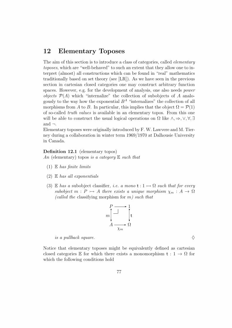
12 Elementary Toposes

The aim of this section is to introduce a class of categories, called elementarytoposes, which are “well-behaved” to such an extent that they allow one to in-terpret (almost) all constructions which can be found in “real” mathematicstraditionally based on set theory (see [LR]). As we have seen in the previoussection in cartesian closed categories one may construct arbitrary functionspaces. However, e.g. for the development of analysis, one also needs powerobjects P(A) which “internalize” the collection of subobjects of A analo-gously to the way how the exponential BA “internalizes” the collection of allmorphisms from A to B. In particular, this implies that the object Ω = P(1)of so-called truth values is available in an elementary topos. From this onewill be able to construct the usual logical operations on Ω like ∧,⇒,∨,∀,∃and ¬.Elementary toposes were originally introduced by F. W. Lawvere and M. Tier-ney during a collaboration in winter term 1969/1970 at Dalhousie Universityin Canada.

Definition 12.1 (elementary topos)An (elementary) topos is a category E such that

(1) E has finite limits

(2) E has all exponentials

(3) E has a subobject classifier, i.e. a mono t : 1 Ω such that for everysubobject m : P A there exists a unique morphism χm : A → Ω(called the classifying morphism for m) such that

P - 1

A

m?

?

χm- Ω

t?

?

is a pullback square. ♦

Notice that elementary toposes might be equivalently defined as cartesianclosed categories E for which there exists a monomorphism t : 1 → Ω forwhich the following conditions hold

77

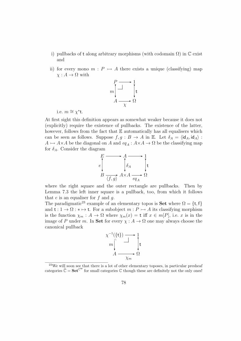
i) pullbacks of t along arbitrary morphisms (with codomain Ω) in C existand

ii) for every mono m : P A there exists a unique (classifying) mapχ : A→ Ω with

P - 1

A

m?

?

χ- Ω

t?

?

i.e. m ∼= χ∗t.

At first sight this definition appears as somewhat weaker because it does not(explicitly) require the existence of pullbacks. The existence of the latter,however, follows from the fact that E automatically has all equalisers whichcan be seen as follows. Suppose f, g : B → A in E. Let δA = 〈idA, idA〉 :A A×A be the diagonal on A and eqA : A×A→ Ω be the classifying mapfor δA. Consider the diagram

E - A - 1

B

e?

?

〈f, g〉- A×A

δA?

?

eqA- Ω

t?

?

where the right square and the outer rectangle are pullbacks. Then byLemma 7.3 the left inner square is a pullback, too, from which it followsthat e is an equaliser for f and g.The paradigmatic23 example of an elementary topos is Set where Ω = t, fand t : 1→ Ω : ∗ 7→ t. For a subobject m : P A its classifying morphismis the function χm : A → Ω where χm(x) = t iff x ∈ m[P ], i.e. x is in theimage of P under m. In Set for every χ : A→ Ω one may always choose thecanonical pullback

χ−1(t) - 1

A

m?

∩

χm- Ω

t?

?

23We will soon see that there is a lot of other elementary toposes, in particular presheafcategories C = SetC

op

for small categories C though these are definitely not the only ones!

78

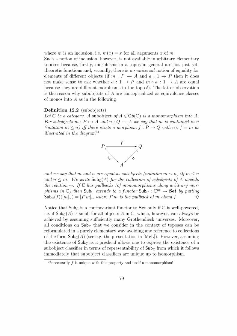
where m is an inclusion, i.e. m(x) = x for all arguments x of m.Such a notion of inclusion, however, is not available in arbitrary elementarytoposes because, firstly, morphisms in a topos in general are not just set-theoretic functions and, secondly, there is no universal notion of equality forelements of different objects (if m : P A and a : 1 → P then it doesnot make sense to ask whether a : 1 → P and m a : 1 → A are equalbecause they are different morphisms in the topos!). The latter observationis the reason why subobjects of A are conceptualized as equivalence classesof monos into A as in the following

Definition 12.2 (subobjects)Let C be a category. A subobject of A ∈ Ob(C) is a monomorphism into A.For subobjects m : P A and n : Q A we say that m is contained in n(notation m ≤ n) iff there exists a morphism f : P → Q with n f = m asillustrated in the diagram24

Pf

- Q

A

n

⊃⊂

m-

and we say that m and n are equal as subobjects (notation m ∼ n) iff m ≤ nand n ≤ m. We write SubC(A) for the collection of subobjects of A modulothe relation ∼. If C has pullbacks (of monomorphisms along arbitrary mor-phisms in C) then SubC extends to a functor SubC : Cop → Set by puttingSubC(f)([m]∼) = [f ∗m]∼ where f ∗m is the pullback of m along f . ♦

Notice that SubC is a contravariant functor to Set only if C is well-powered,i.e. if SubC(A) is small for all objects A in C, which, however, can always beachieved by assuming sufficiently many Grothendieck universes. Moreover,all conditions on SubC that we consider in the context of toposes can bereformulated in a purely elementary way avoiding any reference to collectionsof the form SubC(A) (see e.g. the presentation in [McL]). However, assumingthe existence of SubC as a presheaf allows one to express the existence of asubobject classifier in terms of representability of SubC from which it followsimmediately that subobject classifiers are unique up to isomorphism.

24necessarily f is unique with this property and itself a monomorphism!

79

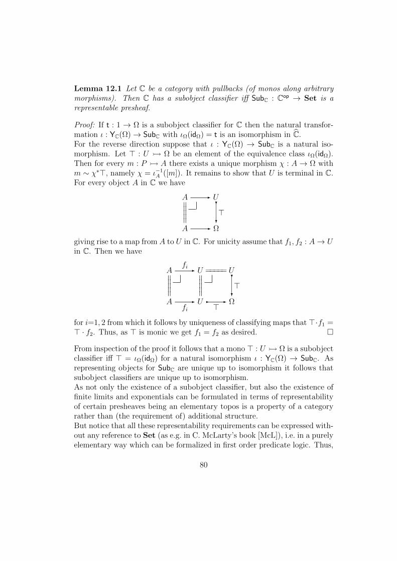
Lemma 12.1 Let C be a category with pullbacks (of monos along arbitrarymorphisms). Then C has a subobject classifier iff SubC : Cop → Set is arepresentable presheaf.

Proof: If t : 1 → Ω is a subobject classifier for C then the natural transfor-mation ι : YC(Ω)→ SubC with ιΩ(idΩ) = t is an isomorphism in C.For the reverse direction suppose that ι : YC(Ω) → SubC is a natural iso-morphism. Let > : U Ω be an element of the equivalence class ιΩ(idΩ).Then for every m : P A there exists a unique morphism χ : A→ Ω withm ∼ χ∗>, namely χ = ι−1

A ([m]). It remains to show that U is terminal in C.For every object A in C we have

A - U

A

wwwww- Ω

>?

?

giving rise to a map from A to U in C. For unicity assume that f1, f2 : A→ Uin C. Then we have

Afi- U ===== U

A

wwwwwfi- U

wwwww->- Ω

>?

?

for i=1, 2 from which it follows by uniqueness of classifying maps that >·f1 => · f2. Thus, as > is monic we get f1 = f2 as desired.

From inspection of the proof it follows that a mono > : U Ω is a subobjectclassifier iff > = ιΩ(idΩ) for a natural isomorphism ι : YC(Ω) → SubC. Asrepresenting objects for SubC are unique up to isomorphism it follows thatsubobject classifiers are unique up to isomorphism.As not only the existence of a subobject classifier, but also the existence offinite limits and exponentials can be formulated in terms of representabilityof certain presheaves being an elementary topos is a property of a categoryrather than (the requirement of) additional structure.But notice that all these representability requirements can be expressed with-out any reference to Set (as e.g. in C. McLarty’s book [McL]), i.e. in a purelyelementary way which can be formalized in first order predicate logic. Thus,

80

the notion of elementary topos is independent from set theory as formalizedby the first order theory ZFC. As we shall see soon toposes are structureswhich are strong enough to perform within them those usual set-theoreticconstructions (cartesian products, function spaces, power sets etc.) that areneeded in the actual practice of modern mathematics (analysis, algebra, ge-ometry etc.). Thus, elementary toposes can be considered as a foundation formathematics alternative to (axiomatic) set theory. This view of foundationshas been forcefully propagated and developed by F. W. Lawvere since middleof 1960ies already. For a most readable textbook account of his view see hisbook Sets for Mathematics (CUP 2003) [LR] together with R. Rosebrugh.The main difference between topos theory and axiomatic set theory lies inthe different choice of basic concepts. In the topos case the basic notions aretypes (objects of the category) and functions between them (morphisms of thecategory) which is in accordance with the practice of modern mathematics.The basic assumption of ZFC is an untyped universe of all sets (which is abit disputable from an ontological point of view!) and a binary relation ∈on this universe of sets telling which sets are elements of which sets. In ZFCfunctions show up as a derived notion, namely as particular sets of pairswhere (following a suggestion of Kuratowski) a pair 〈x, y〉 is “implemented”as the set x, x, y. Natural numbers are also “implemented” (followinga suggestion of J. von Neumann) as 0 = ∅ and n+1 = n ∪ n. All thiskind of coding necessitated by ZFC’s choice of basic notions makes it appearas somewhat artificial in the sense that its basic concepts do not match thebasic concepts of actual mathematical practice.25

A further most useful aspect of topos theory is that it allows for a greatvariety of different models in contrast to ZFC for which it is fairly hard toconstruct different models (as e.g. P. Cohen’s construction26 of forcing modelsfor ZFC where the Continuum Hypothesis fails).The following theorem in one step provides us already with a great varietyof different models for the axioms for an elementary topos.

25Notice, however that set theory is much stronger than (the logic of) toposes even ifthey are boolean, i.e. validate classical logic. The reason is the absence of ZFC’s replace-ment axiom which allows one to transfinitely iterate P. In most of modern mathematicsthis incredible strength of ZFC is not needed at all! However, there are exceptions likeD. Martin’s proof of Borel Determinacy !

26which, by the way, can be given a most understandable explanation in topos theoreticterms (see [MM] but known already in the early 1970ies!)

81

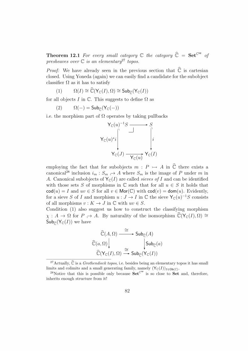
Theorem 12.1 For every small category C the category C = SetCop

ofpresheaves over C is an elementary27 topos.

Proof: We have already seen in the previous section that C is cartesianclosed. Using Yoneda (again) we can easily find a candidate for the subobjectclassifier Ω as it has to satisfy

(1) Ω(I) ∼= C(YC(I),Ω) ∼= SubC(YC(I))

for all objects I in C. This suggests to define Ω as

(2) Ω(−) = SubC(YC(−))

i.e. the morphism part of Ω operates by taking pullbacks

YC(u)−1S - S

YC(J)

YC(u)∗i

?

∩

YC(u)- YC(I)

i

?

∩

employing the fact that for subobjects m : P A in C there exists acanonical28 inclusion im : Sm → A where Sm is the image of P under m inA. Canonical subobjects of YC(I) are called sieves of I and can be identifiedwith those sets S of morphisms in C such that for all u ∈ S it holds thatcod(u) = I and uv ∈ S for all v ∈ Mor(C) with cod(v) = dom(u). Evidently,for a sieve S of I and morphism u : J → I in C the sieve YC(u)−1S consistsof all morphisms v : K → J in C with uv ∈ S.Condition (1) also suggest us how to construct the classifying morphism

χ : A → Ω for P → A. By naturality of the isomorphism C(YC(I),Ω) ∼=SubC(YC(I)) we have

C(A,Ω)∼= - SubC(A)

C(YC(I),Ω)

C(a,Ω)? ∼=- SubC(YC(I))

SubC(a)?

27Actually, C is a Grothendieck topos, i.e. besides being an elementary topos it has smalllimits and colimits and a small generating family, namely (YC(I))I∈Ob(C).

28Notice that this is possible only because SetCop

is so close to Set and, therefore,inherits enough structure from it!

82

for all generalised elements a : YC(I)→ A from which it follows that

(3) χ(a) = a∗P = u : J→I | A(u)(a) ∈ P

according to our identification of Ω(I) with SubC(YC(I)). Condition (3) alsotells us how to construct the subobject classifier t : 1 → Ω. As t is theclassifying map for the subobject id1 : 1→ 1 it follows from (3) that

(4) tI(∗) = >I = u ∈ Mor(C) | cod(u) = I

i.e. t picks the maximal sieve of I for every I ∈ Ob(C).We leave it as a straightforward exercise(!) to the inclined reader to verifythat t : 1 → Ω as defined by (2) and (4) is actually a subobject classifierwhere the construction of classifying maps is given by (3).

Now let us look at Ω in some particular presheaf toposes.29

Example 12.1 If I is a set then Ω in SetI is given by the constant family(0, 1)i∈I where ti(∗) = 0 (assuming that 0 codes “true”). Notice that thisΩ has 2|I| many global elements!

Example 12.2 Let C be the category 0α−→ 1. In C the truth value object

Ω up to isomorphism looks as follows: Ω(1) = f, u, t, Ω(0) = t, f andΩ(α) is the identity on t, f and sends u to t (the “undecided” truth value ucorresponds to the sieve on 1 consisting of just α).

Example 12.3 If C is a monoid M (considered as a category) then Ω con-sists of all right ideals in M , i.e. subsets I of M such that x ∈ I and y ∈Mimplies xy ∈ I, and Ω(x)(I) = y ∈M | xy ∈ I.

Example 12.4 If C is a group G then according to Example 12.3 the truthvalue object Ω of the topos C of G-actions has G, ∅ as underlying set becauseG and ∅ are the only right ideals in G which, moreover, are left invariant byall actions of group elements.

The above examples are already sufficient for exhibiting the relations betweenthe notions introduced in the next definition.

29We leave it as an exercise(!) to explicitate the construction of exponentials in theseexamples!

83

Definition 12.3 (2-valued, boolean, wellpointed)

Let C be a nonempty small category and E = C the corresponding presheaftopos. Let f : 1→ Ω be the classifying map for the subobject 0 1 in E.

• E is 2-valued iff ΩE has precisely 2 global elements, i.e. |E(1,Ω)| = 2.

• E is boolean iff [t, f] : 1+1→ Ω is an isomorphism.

• E is wellpointed iff morphisms f, g : A → B in E are already equalwhenever fa = ga for all global elements a of A, i.e. for all a : 1→ Ain E. ♦

Obviously, for all (nonempty) sets I the topos SetI is boolean but not 2-valued if I contains more than one element. On the other hand for everymonoid M the truth value object Ω of the topos M of right M -actions (seeExample 12.3) contains just 2 global elements, namely M and ∅, (why?) and,accordingly, is 2-valued whereas [t, f] : 1+1→ Ω is not an isomorphism if M

contains non-trivial right ideals (as e.g. the monoid (N,+, 0)), i.e. M is notboolean in such cases. Thus, the properties “2-valued” and “boolean” areindependent in contrast to common superstition!One easily checks that C is 2-valued iff C(J, I) is inhabited for all I, J ∈ C.

First notice that subobjects of 1 in C correspond to sieves in C, i.e. collectionsS of objects in C such that J ∈ S whenever u : J → I and I ∈ S. ThusC is 2-valued iff every nonempty sieve in C coincides with Ob(C). If allhom-sets of C are inhabited then all nonempty sieves in C coincide withOb(C). For the reverse direction consider for every I ∈ C the nonemptysieve SI = J ∈ C | C(J, I) 6= ∅ which by assumption has to coincide withOb(C) and thus all C(J, I) are inhabited.

For every group G the topos G of G-actions is both boolean and 2-valued(see Example 12.4). But if G is nontrivial then G is not wellpointed as therepresentable object G = YG(∗) has then no global elements but admits morethan one endomap (namely, by Yoneda, as many as there are elements in thegroup G).However, if a (presheaf) topos is wellpointed then it is 2-valued and booleanas we shall see next.

Theorem 12.2 Let C be a nonempty small category and E = C the cor-responding presheaf topos. Then E is 2-valued and boolean whenever E iswellpointed.

84

Proof: Assume that E = C is wellpointed.Suppose E is not 2-valued, i.e. there exists a further global element u : 1→ Ωbesides t and f. Let i : U 1 be the subobject classified by u. The mapst i and f i are different as they classify different subobjects of U , namelyU and 0, respectively. Thus, by wellpointedness there exists a global elementu : 1→ U separating t i and f i. Obviously, the map u is an isomorphismfrom which it follows that U ∼= 1 in contradiction to the assumption t 6= u.Thus E is 2-valued.Let χ : Ω→ Ω be the classifying map for the monomorphism [t, f] : 1+1 Ω.As t, f ≤Ω [t, f] it follows that t∗[t, f] ∼= id1

∼= f∗[t, f]. Thus χ t = t = χ ffrom which it follows by wellpointedness that χ = t !Ω. Thus, we have[t, f] ∼= idΩ and, accordingly, the map [t, f] is an isomorphism, i.e. the toposE is boolean.

Notice that Definition 12.3 makes sense already for arbitrary elementarytoposes because one can show (see e.g. [MM]) that they have all finite colim-its, that 0 1 and that [t, f] : 1+1 Ω. Moreover, wellpointed elementarytoposes all have the following property which makes them behave like Henkinmodels for higher order logic (see Chapter 13)

Lemma 12.2 If E is a wellpointed topos then non-initial objects of E haveglobal elements.

Proof: Suppose A is an object of E. The unique morphism 0→ A is a monoclassified by f and it is an isomorphism iff A is initial. Thus A is non-initialiff tA = t!A and fA = t!A are different in which case by wellpointedness ofA there exists an a : 1→ A with tA a 6= fA a.

A topos E is called localic if the subobjects of 1E constitute a generatingfamily for E. Typical examples are presheaf toposes of the form P where P isa posetal category as e.g. the one considered in Example 12.2. One readilychecks (reusing the second part of the proof of Theorem 12.2) that if a localictopos is 2-valued then it is also boolean.Finally, we leave it as an exercise(!) to show that for small categories C the

presheaf topos C is boolean iff C is a groupoid, i.e. all morphisms in C are isos.Thus C is boolean and 2-valued iff C is a connected groupoid (“connected”meaning that all homsets of C are inhabited). As SetI is wellpointed iff

|I| = 1 (why?) it follows that C is wellpointed if and only if C is equivalentto 1, the trivial nonempty category.

85

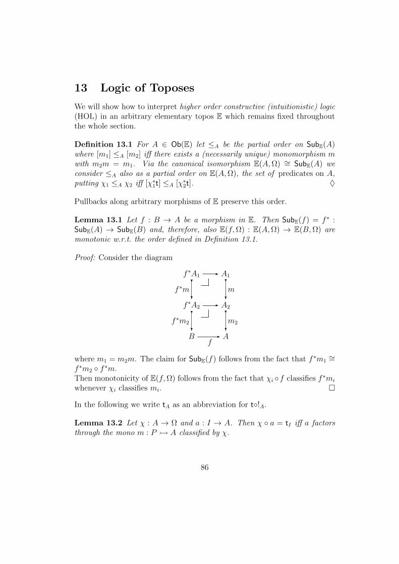
13 Logic of Toposes

We will show how to interpret higher order constructive (intuitionistic) logic(HOL) in an arbitrary elementary topos E which remains fixed throughoutthe whole section.

Definition 13.1 For A ∈ Ob(E) let ≤A be the partial order on SubE(A)where [m1] ≤A [m2] iff there exists a (necessarily unique) monomorphism mwith m2m = m1. Via the canonical isomorphism E(A,Ω) ∼= SubE(A) weconsider ≤A also as a partial order on E(A,Ω), the set of predicates on A,putting χ1 ≤A χ2 iff [χ∗1t] ≤A [χ∗2t]. ♦

Pullbacks along arbitrary morphisms of E preserve this order.

Lemma 13.1 Let f : B → A be a morphism in E. Then SubE(f) = f ∗ :SubE(A) → SubE(B) and, therefore, also E(f,Ω) : E(A,Ω) → E(B,Ω) aremonotonic w.r.t. the order defined in Definition 13.1.

Proof: Consider the diagram

f ∗A1- A1

f ∗A2

f ∗m?

?

- A2

m?

?

B

f ∗m2?

?

f- A

m2?

?

where m1 = m2m. The claim for SubE(f) follows from the fact that f ∗m1∼=

f ∗m2 f ∗m.Then monotonicity of E(f,Ω) follows from the fact that χi f classifies f ∗mi

whenever χi classifies mi.

In the following we write tA as an abbreviation for t!A.

Lemma 13.2 Let χ : A → Ω and a : I → A. Then χ a = tI iff a factorsthrough the mono m : P A classified by χ.

86

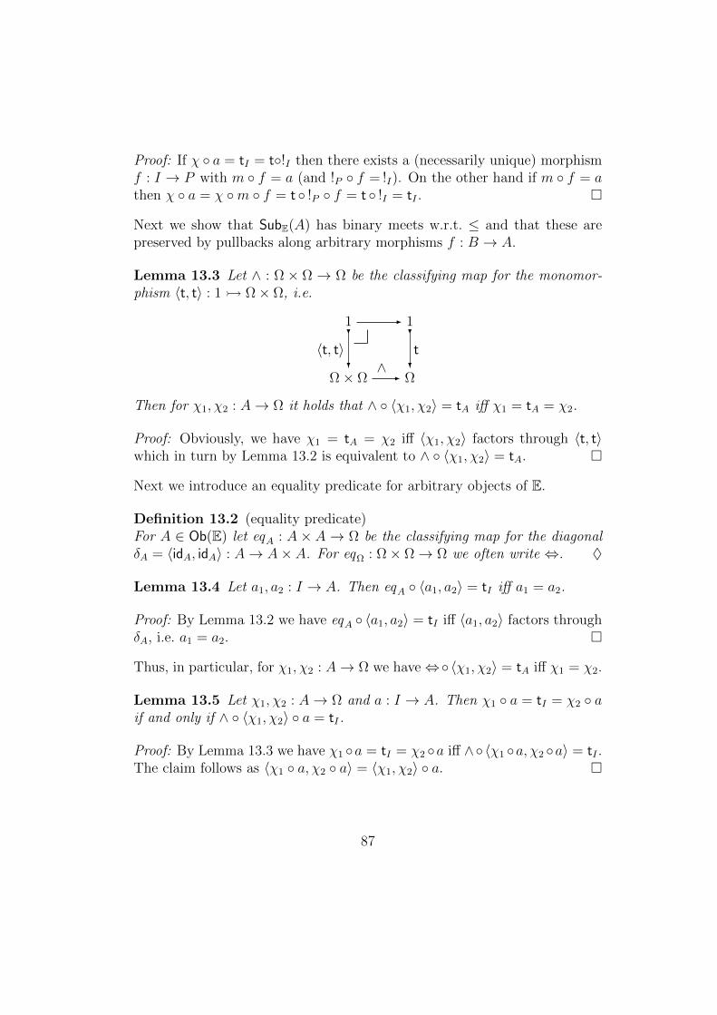
Proof: If χ a = tI = t!I then there exists a (necessarily unique) morphismf : I → P with m f = a (and !P f = !I). On the other hand if m f = athen χ a = χ m f = t !P f = t !I = tI .

Next we show that SubE(A) has binary meets w.r.t. ≤ and that these arepreserved by pullbacks along arbitrary morphisms f : B → A.

Lemma 13.3 Let ∧ : Ω × Ω → Ω be the classifying map for the monomor-phism 〈t, t〉 : 1 Ω× Ω, i.e.

1 - 1

Ω× Ω

〈t, t〉?

?

∧- Ω

t?

?

Then for χ1, χ2 : A→ Ω it holds that ∧ 〈χ1, χ2〉 = tA iff χ1 = tA = χ2.

Proof: Obviously, we have χ1 = tA = χ2 iff 〈χ1, χ2〉 factors through 〈t, t〉which in turn by Lemma 13.2 is equivalent to ∧ 〈χ1, χ2〉 = tA.

Next we introduce an equality predicate for arbitrary objects of E.

Definition 13.2 (equality predicate)For A ∈ Ob(E) let eqA : A× A→ Ω be the classifying map for the diagonalδA = 〈idA, idA〉 : A→ A× A. For eqΩ : Ω× Ω→ Ω we often write ⇔. ♦

Lemma 13.4 Let a1, a2 : I → A. Then eqA 〈a1, a2〉 = tI iff a1 = a2.

Proof: By Lemma 13.2 we have eqA 〈a1, a2〉 = tI iff 〈a1, a2〉 factors throughδA, i.e. a1 = a2.

Thus, in particular, for χ1, χ2 : A→ Ω we have⇔〈χ1, χ2〉 = tA iff χ1 = χ2.

Lemma 13.5 Let χ1, χ2 : A→ Ω and a : I → A. Then χ1 a = tI = χ2 aif and only if ∧ 〈χ1, χ2〉 a = tI .

Proof: By Lemma 13.3 we have χ1 a = tI = χ2 a iff ∧〈χ1 a, χ2 a〉 = tI .The claim follows as 〈χ1 a, χ2 a〉 = 〈χ1, χ2〉 a.

87

Theorem 13.1 (conjunction)For every A ∈ Ob(E) the poset SubE(A) is a ∧-semilattice w.r.t. ≤, i.e.has finite infima, that are preserved by SubE(f) : SubE(A) → SubE(B) forarbitrary morphisms f : B → A in E. Moreover, if χ1, χ2 : A → Ω classifysubobjects m1 : P1 A and m2 : P2 A, respectively, then ∧ 〈χ1, χ2〉classifies the infimum of m1 and m2.

Proof: Let χ1 and χ2 be the classifying maps for m1 and m2, respectively.Let m : P A be the subobject classified by ∧ 〈χ1, χ2〉. We show thatm is the infimum of m1 and m2. By Lemma 13.2 and Lemma 13.5 for alln : Q A we have n ≤A m iff ∧ 〈χ1, χ2〉 n = tQ iff χ1 n = tQ andχ2 n = tQ iff n ≤A m1 and n ≤A m2. Thus m = m1 ∧m2 as desired.Now suppose f : B → A. Then ∧ 〈χ1, χ2〉 f = ∧ 〈χ1 f, χ2 f〉 classifiesboth f ∗m and the infimum of f ∗m1 and f ∗m2. Thus f ∗ preserves meets ofsubobjects.

Instead of ∧ 〈χ1, χ2〉 we usually write χ1 ∧ χ2 in accordance with the factthat it is the infimum of χ1 and χ2 in E(A,Ω).

Next we introduce implication as a binary operation on Ω.

Definition 13.3 (implication)Let ⇒ : Ω × Ω → Ω be defined as ⇔ 〈∧, π1〉 where π1 : Ω × Ω → Ω is theprojection on the first component. ♦

Again, for reasons of readability, we often write χ1⇒χ2 as an abbreviationfor ⇒ 〈χ1, χ2〉.

Lemma 13.6 Let χ1, χ2 : A→ Ω then χ1 ≤A χ2 iff ⇒ 〈χ1, χ2〉 = tA.

Proof: For χ1, χ2 : A→ Ω we have

⇒ 〈χ1, χ2〉 = tA iff (Lemma 13.4)

∧ 〈χ1, χ2〉 = χ1 iff

χ1 ≤A χ2

where the second equality follows from the fact that in arbitrary posets x ≤ yiff x is the infimum of x and y.

88

Lemma 13.7 For maps χ1, χ2 and χ from A to Ω we have

χ ∧ χ1 ≤A χ2 iff χ ≤A χ1⇒χ2 .

Proof: Let m : P A, m1 : P1 A and m2 : P2 A be the subobjectsclassified by χ, χ1 and χ2, respectively. Then we have

χ ≤A χ1⇒χ2 iff (Lemma 13.2)

(χ1⇒χ2) m = tP iff (Lemma 13.6)

χ1 m ≤P χ2 m iff (χi m classifies m∗mi)

m∗m1 ≤ m∗m2 iff (m (−) order reflecting)

m m∗m1 ≤ m m∗m2 iff (m m∗mi∼= m ∧mi)

m ∧m1 ≤A m ∧m2 iff (as m ∧m1 ≤A m holds anyway)

m ∧m1 ≤A m2 iff (as m ∧m1 is classified by χ ∧ χ1)

χ ∧ χ1 ≤A χ2

i.e. the poset SubE(A) has Heyting implication30.

Notice that pullback functors f ∗ preserve Heyting implication because wehave ⇒ 〈χ1, χ2〉 a = ⇒ 〈χ1 a, χ2 a〉 for arbitrary a : I → A.

Summarizing we have

Theorem 13.2 In E every SubE(A) is a poset with finite infima and Heytingimplication which structure is preserved by f−1 : SubE(A)→ SubE(B) for allf : B → A in E.

Proof: For conjunctions and implication the claim is immediate from theprevious lemmas. Every SubE(A) has a greatest element idA classified bytA. Preservation of greatest elements is immediate from tA f = tB for allf : B → A.

Next we will introduce universal quantification over objects in E.

30A poset H with binary meets admits Heyting implication iff for all a, b ∈ H thereexists a necessarily unique a⇒b ∈ H such that

x ≤ a⇒b iff x ∧ a ≤ b

for all x ∈ H.

89

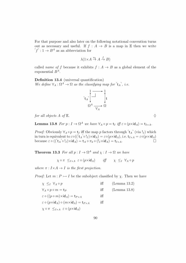
For that purpose and also later on the following notational convention turnsout as necessary and useful. If f : A → B is a map in E then we writepfq : 1→ BA as an abbreviation for

λ(1×A π2→ Af→ B)

called name of f because it exhibits f : A → B as a global element of theexponential BA.

Definition 13.4 (universal quantification)We define ∀A : ΩA → Ω as the classifying map for ptA

q, i.e.

1 - 1

ΩA

ptAq

?

?

∀A- Ω

t?

?

for all objects A of E. ♦

Lemma 13.8 For p : I → ΩA we have ∀A p = tI iff ε (p×idA) = tI×A.

Proof: Obviously ∀A p = tI iff the map p factors through ptAq (via !I) which

in turn is equivalent to ε((ptAq !I)×idA) = ε(p×idA), i.e. tI×A = ε(p×idA)because ε ((ptA

q !I)×idA) = tA π2 (!I×idA) = tI×A.

Theorem 13.3 For all p : I → ΩA and χ : I → Ω we have

χ π ≤I×A ε (p×idA) iff χ ≤I ∀A p

where π : I×A→ I is the first projection.

Proof: Let m : P I be the subobject classified by χ. Then we have

χ ≤I ∀A p iff (Lemma 13.2)

∀A p m = tP iff (Lemma 13.8)

ε ((p m)×idA) = tP×A iff

ε (p×idA) (m×idA) = tP×A iff

χ π ≤I×A ε (p×idA)

90

where the last equivalence follows from Lemma 13.2) and the fact that χ πclassifies the subobject m×idA (as (χπ)∗t ∼= π∗χ∗t = π∗m = m×idA).

The following equivalent variant of Theorem 13.3 will turn out as more usefulwhen we consider proof rules for the internal logic.

Theorem 13.4 Let ϕ : I×A → Ω and ψ : I → Ω be maps in E. Then for∀A(ϕ) := ∀A λ(ϕ) it holds that

ψ π ≤I×A ϕ iff ψ ≤I ∀A(ϕ)

where π : I × A→ I is the first projection.

Proof: Immediate from Theorem 13.3 instantiating p by λ(ϕ).

The Internal Language

We have seen that in an elementary topos E one can interpret the logicaloperations > (truth), ∧ (conjunction), ⇒ (implication) and ∀A (universalquantification over A). We next will introduce a formal language, calledinternal language of E 31, which is based on typed λ-calculus and containsconstants for denoting the objects and morphisms of E including the abovementioned logical operations >, ∧, ⇒ and ∀A.More precisely, the internal language of E is the typed λ-calculus over thecollection Ob(E) of base types augmented by a constant of type BA for ev-ery morphism f : A → B. As E is cartesian closed it is obvious how tointerpret the internal language of E in the cartesian closed category E (aconstant for object A will be interpreted as A and a constant for morphismf : A → B will be interpreted as pfq : 1 → BA). The terms Γ ` ϕ : Ω oftype Ω in context Γ are called propositions in context Γ and will be inter-preted as morphisms [[Γ]]→ ΩE, i.e. as subobjects of [[Γ]] via the isomorphismSubE([[Γ]]) ∼= E([[Γ]],ΩE). If Γ is a context and Γ ` ϕi : Ω (i=1, . . . , n) andΓ ` ϕ : Ω are propositions in context Γ then we write

Γ | ϕ1, . . . , ϕn ` ϕ31The internal language of E is also often called the Mitchell-Benabou language because

the internal language was introduced beginning of the 1970ies originally by Jean Benabouand later (independently) by W. Mitchell.

91

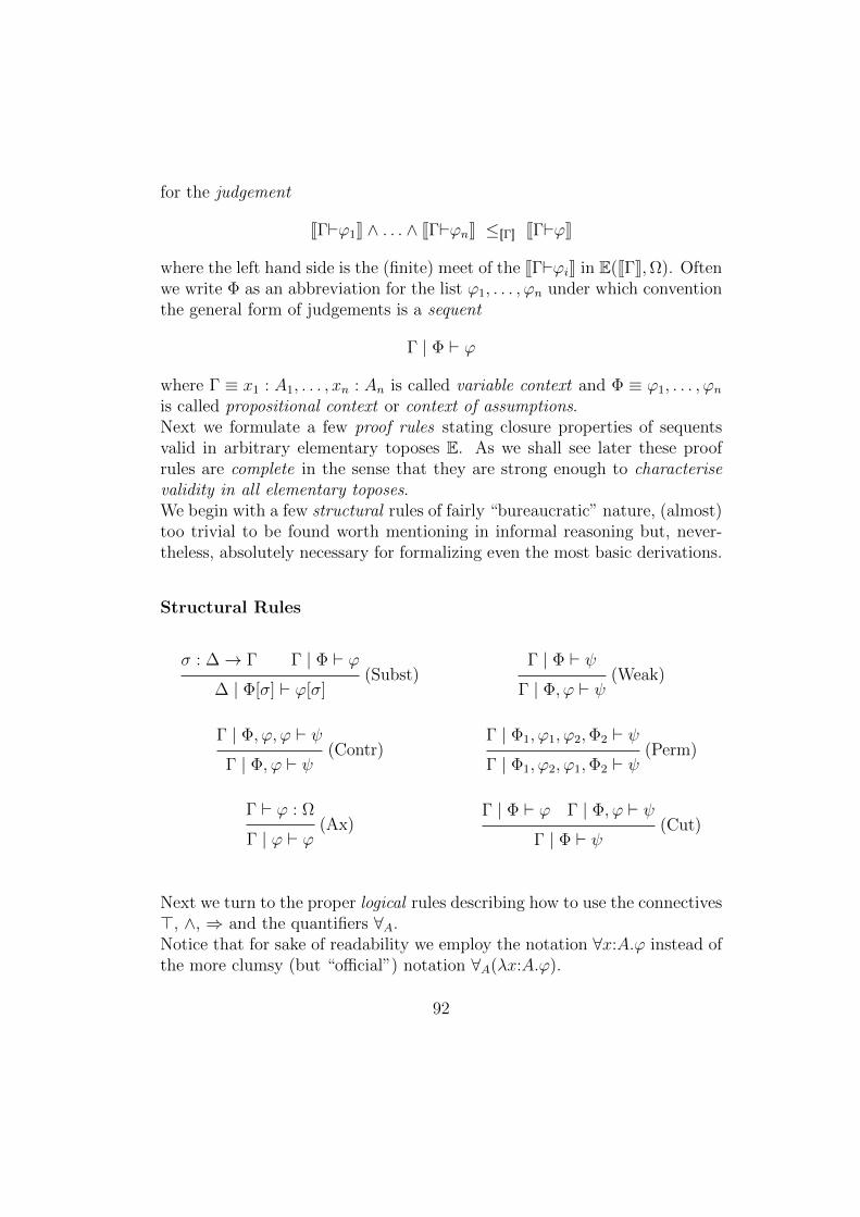
for the judgement

[[Γ`ϕ1]] ∧ . . . ∧ [[Γ`ϕn]] ≤[[Γ]] [[Γ`ϕ]]

where the left hand side is the (finite) meet of the [[Γ`ϕi]] in E([[Γ]],Ω). Oftenwe write Φ as an abbreviation for the list ϕ1, . . . , ϕn under which conventionthe general form of judgements is a sequent

Γ | Φ ` ϕ

where Γ ≡ x1 : A1, . . . , xn : An is called variable context and Φ ≡ ϕ1, . . . , ϕnis called propositional context or context of assumptions.Next we formulate a few proof rules stating closure properties of sequentsvalid in arbitrary elementary toposes E. As we shall see later these proofrules are complete in the sense that they are strong enough to characterisevalidity in all elementary toposes.We begin with a few structural rules of fairly “bureaucratic” nature, (almost)too trivial to be found worth mentioning in informal reasoning but, never-theless, absolutely necessary for formalizing even the most basic derivations.

Structural Rules

σ : ∆→ Γ Γ | Φ ` ϕ(Subst)

∆ | Φ[σ] ` ϕ[σ]

Γ | Φ ` ψ(Weak)

Γ | Φ, ϕ ` ψ

Γ | Φ, ϕ, ϕ ` ψ(Contr)

Γ | Φ, ϕ ` ψ

Γ | Φ1, ϕ1, ϕ2,Φ2 ` ψ(Perm)

Γ | Φ1, ϕ2, ϕ1,Φ2 ` ψ

Γ ` ϕ : Ω(Ax)

Γ | ϕ ` ϕΓ | Φ ` ϕ Γ | Φ, ϕ ` ψ

(Cut)Γ | Φ ` ψ

Next we turn to the proper logical rules describing how to use the connectives>, ∧, ⇒ and the quantifiers ∀A.Notice that for sake of readability we employ the notation ∀x:A.ϕ instead ofthe more clumsy (but “official”) notation ∀A(λx:A.ϕ).

92

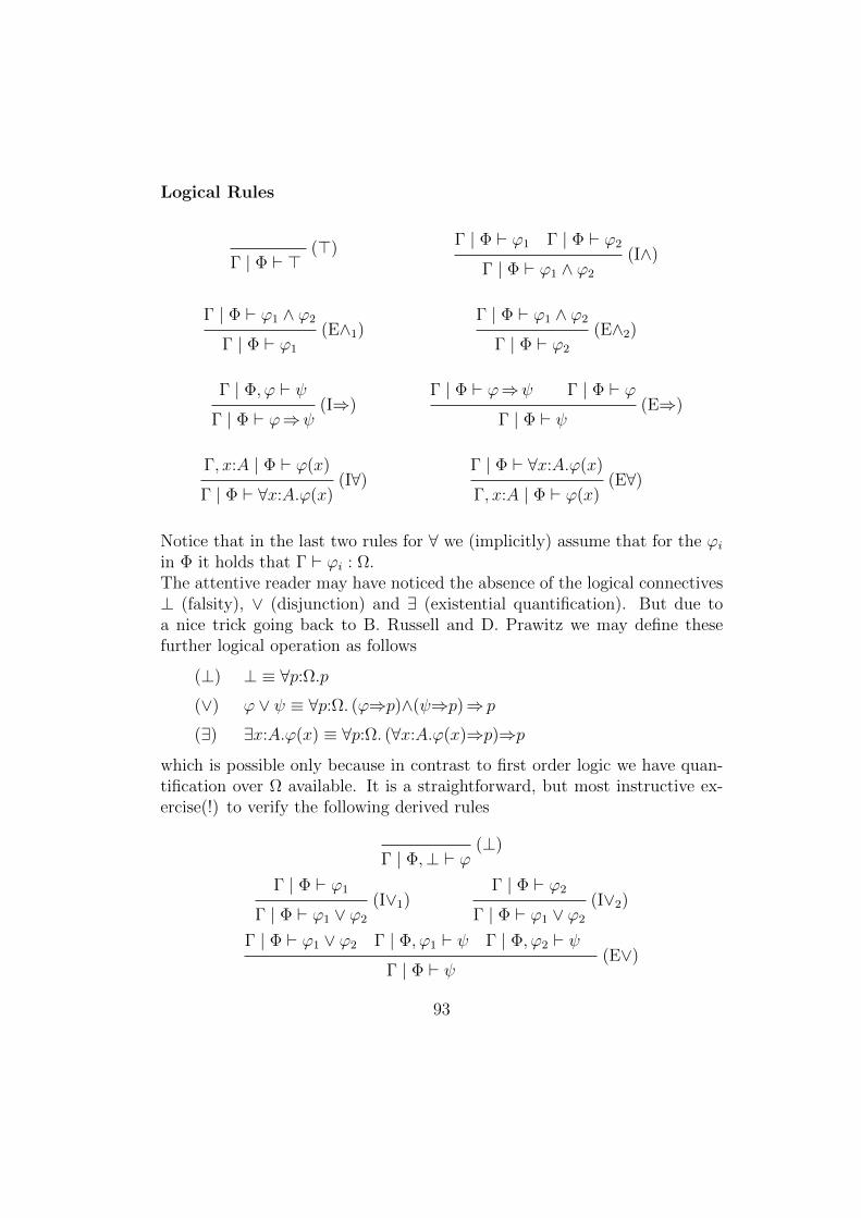
Logical Rules

(>)Γ | Φ ` >

Γ | Φ ` ϕ1 Γ | Φ ` ϕ2(I∧)

Γ | Φ ` ϕ1 ∧ ϕ2

Γ | Φ ` ϕ1 ∧ ϕ2(E∧1)

Γ | Φ ` ϕ1

Γ | Φ ` ϕ1 ∧ ϕ2(E∧2)

Γ | Φ ` ϕ2

Γ | Φ, ϕ ` ψ(I⇒)

Γ | Φ ` ϕ⇒ψ

Γ | Φ ` ϕ⇒ψ Γ | Φ ` ϕ(E⇒)

Γ | Φ ` ψ

Γ, x:A | Φ ` ϕ(x)(I∀)

Γ | Φ ` ∀x:A.ϕ(x)

Γ | Φ ` ∀x:A.ϕ(x)(E∀)

Γ, x:A | Φ ` ϕ(x)

Notice that in the last two rules for ∀ we (implicitly) assume that for the ϕiin Φ it holds that Γ ` ϕi : Ω.The attentive reader may have noticed the absence of the logical connectives⊥ (falsity), ∨ (disjunction) and ∃ (existential quantification). But due toa nice trick going back to B. Russell and D. Prawitz we may define thesefurther logical operation as follows

(⊥) ⊥ ≡ ∀p:Ω.p(∨) ϕ ∨ ψ ≡ ∀p:Ω. (ϕ⇒p)∧(ψ⇒p)⇒ p

(∃) ∃x:A.ϕ(x) ≡ ∀p:Ω. (∀x:A.ϕ(x)⇒p)⇒p

which is possible only because in contrast to first order logic we have quan-tification over Ω available. It is a straightforward, but most instructive ex-ercise(!) to verify the following derived rules

(⊥)Γ | Φ,⊥ ` ϕ

Γ | Φ ` ϕ1(I∨1)

Γ | Φ ` ϕ1 ∨ ϕ2

Γ | Φ ` ϕ2(I∨2)

Γ | Φ ` ϕ1 ∨ ϕ2

Γ | Φ ` ϕ1 ∨ ϕ2 Γ | Φ, ϕ1 ` ψ Γ | Φ, ϕ2 ` ψ(E∨)

Γ | Φ ` ψ

93

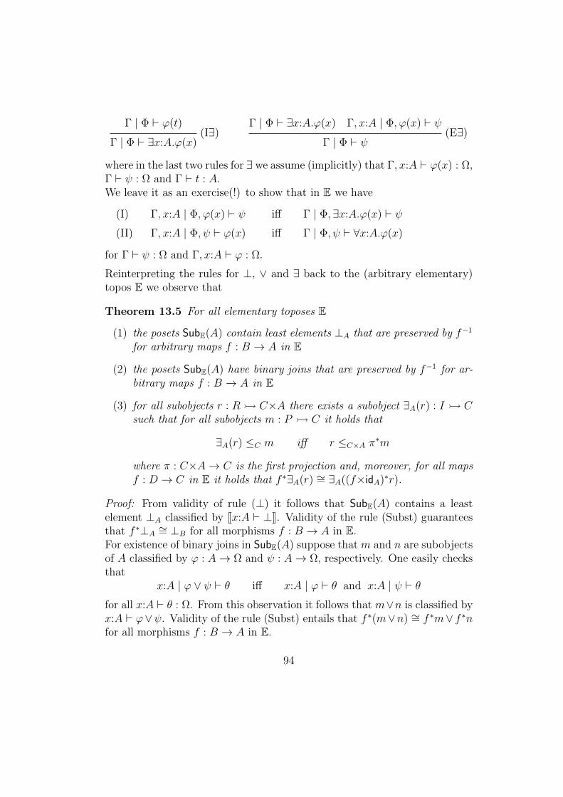
Γ | Φ ` ϕ(t)(I∃)

Γ | Φ ` ∃x:A.ϕ(x)

Γ | Φ ` ∃x:A.ϕ(x) Γ, x:A | Φ, ϕ(x) ` ψ(E∃)

Γ | Φ ` ψ

where in the last two rules for ∃ we assume (implicitly) that Γ, x:A ` ϕ(x) : Ω,Γ ` ψ : Ω and Γ ` t : A.We leave it as an exercise(!) to show that in E we have

(I) Γ, x:A | Φ, ϕ(x) ` ψ iff Γ | Φ,∃x:A.ϕ(x) ` ψ(II) Γ, x:A | Φ, ψ ` ϕ(x) iff Γ | Φ, ψ ` ∀x:A.ϕ(x)

for Γ ` ψ : Ω and Γ, x:A ` ϕ : Ω.

Reinterpreting the rules for ⊥, ∨ and ∃ back to the (arbitrary elementary)topos E we observe that

Theorem 13.5 For all elementary toposes E

(1) the posets SubE(A) contain least elements ⊥A that are preserved by f−1

for arbitrary maps f : B → A in E

(2) the posets SubE(A) have binary joins that are preserved by f−1 for ar-bitrary maps f : B → A in E

(3) for all subobjects r : R C×A there exists a subobject ∃A(r) : I Csuch that for all subobjects m : P C it holds that

∃A(r) ≤C m iff r ≤C×A π∗m

where π : C×A→ C is the first projection and, moreover, for all mapsf : D → C in E it holds that f ∗∃A(r) ∼= ∃A((f×idA)∗r).

Proof: From validity of rule (⊥) it follows that SubE(A) contains a leastelement ⊥A classified by [[x:A ` ⊥]]. Validity of the rule (Subst) guaranteesthat f ∗⊥A ∼= ⊥B for all morphisms f : B → A in E.For existence of binary joins in SubE(A) suppose that m and n are subobjectsof A classified by ϕ : A→ Ω and ψ : A→ Ω, respectively. One easily checksthat

x:A | ϕ ∨ ψ ` θ iff x:A | ϕ ` θ and x:A | ψ ` θfor all x:A ` θ : Ω. From this observation it follows that m∨n is classified byx:A ` ϕ∨ψ. Validity of the rule (Subst) entails that f ∗(m∨n) ∼= f ∗m∨ f ∗nfor all morphisms f : B → A in E.

94

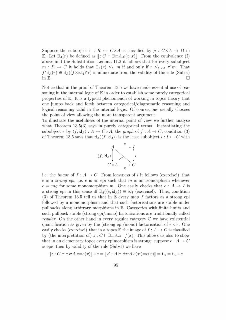
Suppose the subobject r : R C×A is classified by ρ : C×A → Ω inE. Let ∃A(r) be defined as [[z:C ` ∃x:A.ρ(z, x)]]. From the equivalence (I)above and the Substitution Lemma 11.2 it follows that for every subobjectm : P C it holds that ∃A(r) ≤C m if and only if r ≤C×A π∗m. Thatf ∗∃A(r) ∼= ∃A((f×idA)∗r) is immediate from the validity of the rule (Subst)in E.

Notice that in the proof of Theorem 13.5 we have made essential use of rea-soning in the internal logic of E in order to establish some purely categoricalproperties of E. It is a typical phenomenon of working in topos theory thatone jumps back and forth between categorical/diagramatic reasoning andlogical reasoning valid in the internal logic. Of course, one usually choosesthe point of view allowing the more transparent argument.To illustrate the usefulness of the internal point of view we further analysewhat Theorem 13.5(3) says in purely categorical terms. Instantiating thesubobject r by 〈f, idA〉 : A C×A, the graph of f : A → C, condition (3)of Theorem 13.5 says that ∃A(〈f, idA〉) is the least subobject i : I C with

Ae- I

C×A

〈f, idA〉?

?

π- C

i?

?

f -

i.e. the image of f : A → C. From leastness of i it follows (exercise!) thate is a strong epi, i.e. e is an epi such that m is an isomorphism whenevere = mg for some monomorphism m. One easily checks that e : A → I isa strong epi in this sense iff ∃A(〈e, idA〉) ∼= idI (exercise!). Thus, condition(3) of Theorem 13.5 tell us that in E every map f factors as a strong epifollowed by a monomorphism and that such factorisations are stable underpullbacks along arbitrary morphisms in E. Categories with finite limits andsuch pullback stable (strong epi/mono) factorisations are traditionally calledregular. On the other hand in every regular category C we have existentialquantification as given by the (strong epi/mono) factorisation of π r. Oneeasily checks (exercise!) that in a topos E the image of f : A→ C is classifiedby (the interpretation of) z : C ` ∃x:A.z=f(x). This allows us also to showthat in an elementary topos every epimorphism is strong: suppose e : A Cis epic then by validity of the rule (Subst) we have

[[z : C ` ∃x:A.z=e(x)]] e = [[x′ : A ` ∃x:A.e(x′)=e(x)]] = tA = tC e

95

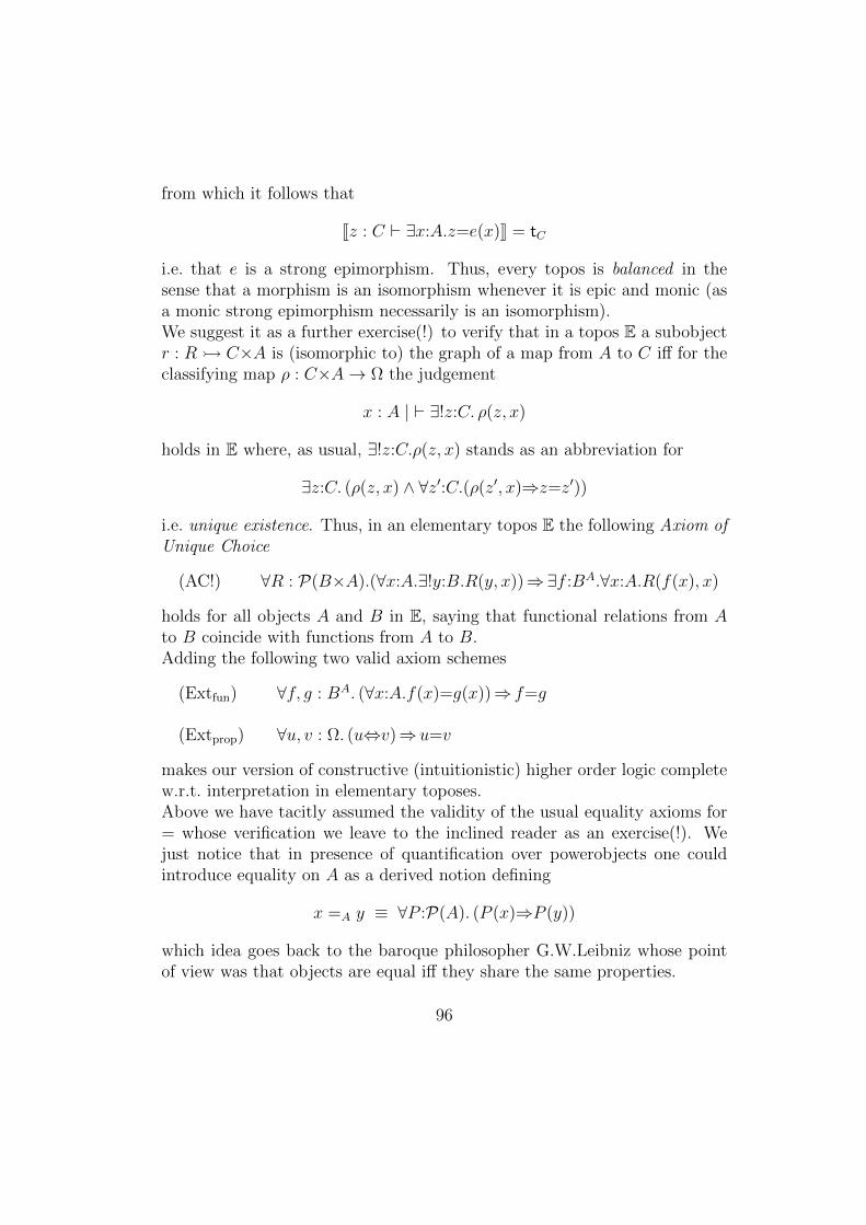
from which it follows that

[[z : C ` ∃x:A.z=e(x)]] = tC

i.e. that e is a strong epimorphism. Thus, every topos is balanced in thesense that a morphism is an isomorphism whenever it is epic and monic (asa monic strong epimorphism necessarily is an isomorphism).We suggest it as a further exercise(!) to verify that in a topos E a subobjectr : R C×A is (isomorphic to) the graph of a map from A to C iff for theclassifying map ρ : C×A→ Ω the judgement

x : A | ` ∃!z:C. ρ(z, x)

holds in E where, as usual, ∃!z:C.ρ(z, x) stands as an abbreviation for

∃z:C. (ρ(z, x) ∧ ∀z′:C.(ρ(z′, x)⇒z=z′))

i.e. unique existence. Thus, in an elementary topos E the following Axiom ofUnique Choice

(AC!) ∀R : P(B×A).(∀x:A.∃!y:B.R(y, x))⇒∃f :BA.∀x:A.R(f(x), x)

holds for all objects A and B in E, saying that functional relations from Ato B coincide with functions from A to B.Adding the following two valid axiom schemes

(Extfun) ∀f, g : BA. (∀x:A.f(x)=g(x))⇒ f=g

(Extprop) ∀u, v : Ω. (u⇔v)⇒u=v

makes our version of constructive (intuitionistic) higher order logic completew.r.t. interpretation in elementary toposes.Above we have tacitly assumed the validity of the usual equality axioms for= whose verification we leave to the inclined reader as an exercise(!). Wejust notice that in presence of quantification over powerobjects one couldintroduce equality on A as a derived notion defining

x =A y ≡ ∀P :P(A). (P (x)⇒P (y))

which idea goes back to the baroque philosopher G.W.Leibniz whose pointof view was that objects are equal iff they share the same properties.

96

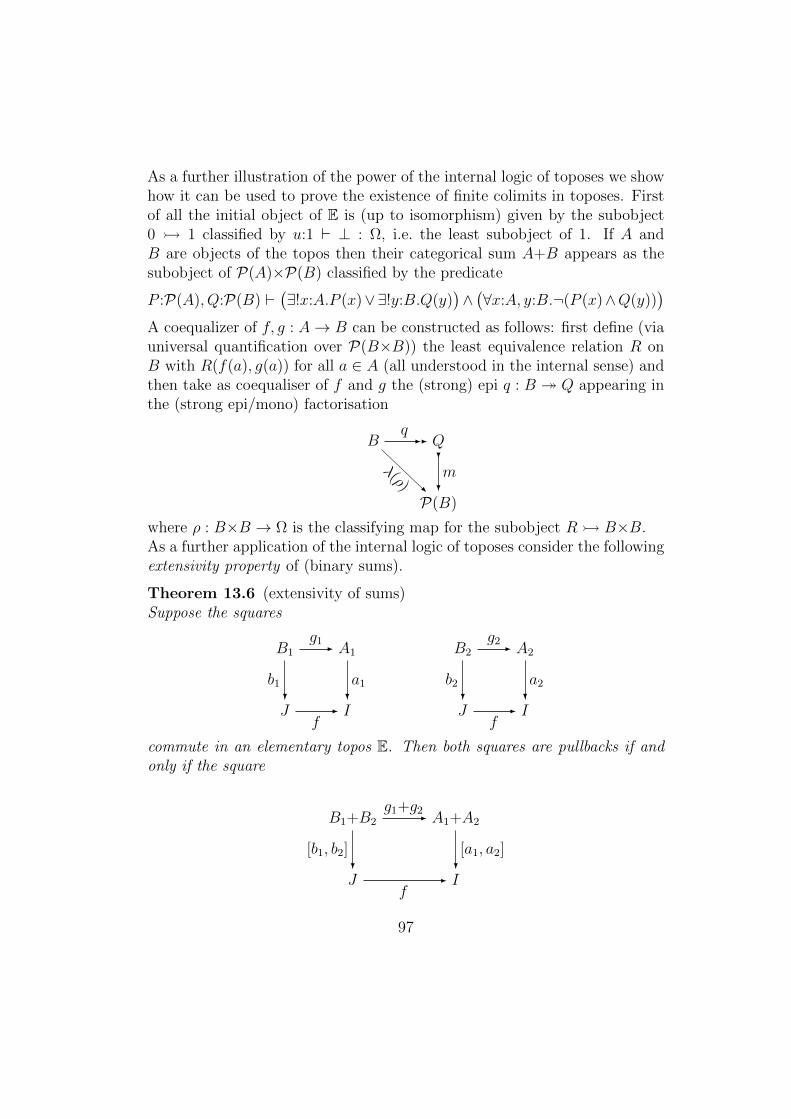
As a further illustration of the power of the internal logic of toposes we showhow it can be used to prove the existence of finite colimits in toposes. Firstof all the initial object of E is (up to isomorphism) given by the subobject0 1 classified by u:1 ` ⊥ : Ω, i.e. the least subobject of 1. If A andB are objects of the topos then their categorical sum A+B appears as thesubobject of P(A)×P(B) classified by the predicate

P :P(A), Q:P(B) `(∃!x:A.P (x)∨∃!y:B.Q(y)

)∧(∀x:A, y:B.¬(P (x)∧Q(y))

)A coequalizer of f, g : A→ B can be constructed as follows: first define (viauniversal quantification over P(B×B)) the least equivalence relation R onB with R(f(a), g(a)) for all a ∈ A (all understood in the internal sense) andthen take as coequaliser of f and g the (strong) epi q : B Q appearing inthe (strong epi/mono) factorisation

Bq-- Q

P(B)

m?

?λ(ρ) -

where ρ : B×B → Ω is the classifying map for the subobject R B×B.As a further application of the internal logic of toposes consider the followingextensivity property of (binary sums).

Theorem 13.6 (extensivity of sums)Suppose the squares

B1

g1- A1 B2

g2- A2

J

b1?

f- I

a1?

J

b2?

f- I

a2?

commute in an elementary topos E. Then both squares are pullbacks if andonly if the square

B1+B2

g1+g2- A1+A2

J

[b1, b2]?

f- I

[a1, a2]?

97

is a pullback.

Proof: Employ the following construction of pullbacks using the internal logicof E : given maps f : A → C and g : B → C in E then their pullback isgiven by the subobject P A×B classified by x:A, y:B ` f(x) =C g(y).Details are left to the reader.

Kripke-Joyal Semantics

We have seen already how to interpret higher order logic in a topos where aformula ϕ in context x1 : A1, . . . , xn : An gets interpreted as a subobject ofA1×· · ·×An.32 This has the disadvantage that the most pleasant illusion of“elements” is totally lost. Well, for non-wellpointed toposes E one certainlydoesn’t know a predicate ϕ : A → Ω when knowing the collection of globalpoints a : 1→ A of A with ϕa = t. But, obviously, the predicate ϕ : A→ Ωis fully determined by the collection of all generalised elements a : I → Asatisfying ϕ (notation a ϕ), i.e. ϕ a = tI . Now Kripke-Joyal semanticsexploits this observation by specifying (by structural recursion over ϕ) thecollection of all generalised elements a with a ϕ thus reestablishing theform of the Tarskian definition of truth.Before giving the clauses of the Kripke-Joyal semantics we state the followingtwo principles holding for (often called forcing relation)

Monotonicity If a ϕ for a : I → A and f : J → I then af ϕ

Local Character If a : I → A and e : J I epic with ae ϕ then a ϕ.

whose straightforward verification we leave as an exercise(!) for the reader.

Theorem 13.7 (Truth Conditions a la Kripke-Joyal)In an elementary topos E for predicates ϕ, ψ : A → Ω and generalized ele-ments a : I → A we have that

(>) a tA always holds

(∧) a ϕ ∧ ψ iff a ϕ and a ψ

32Notice that at least from now on we often drop the semantic brackets [[·]] when theyare clear from the context. Moreover, in the end the distinction between object andmetalanguage is not the greatest insight of logic after all!

98

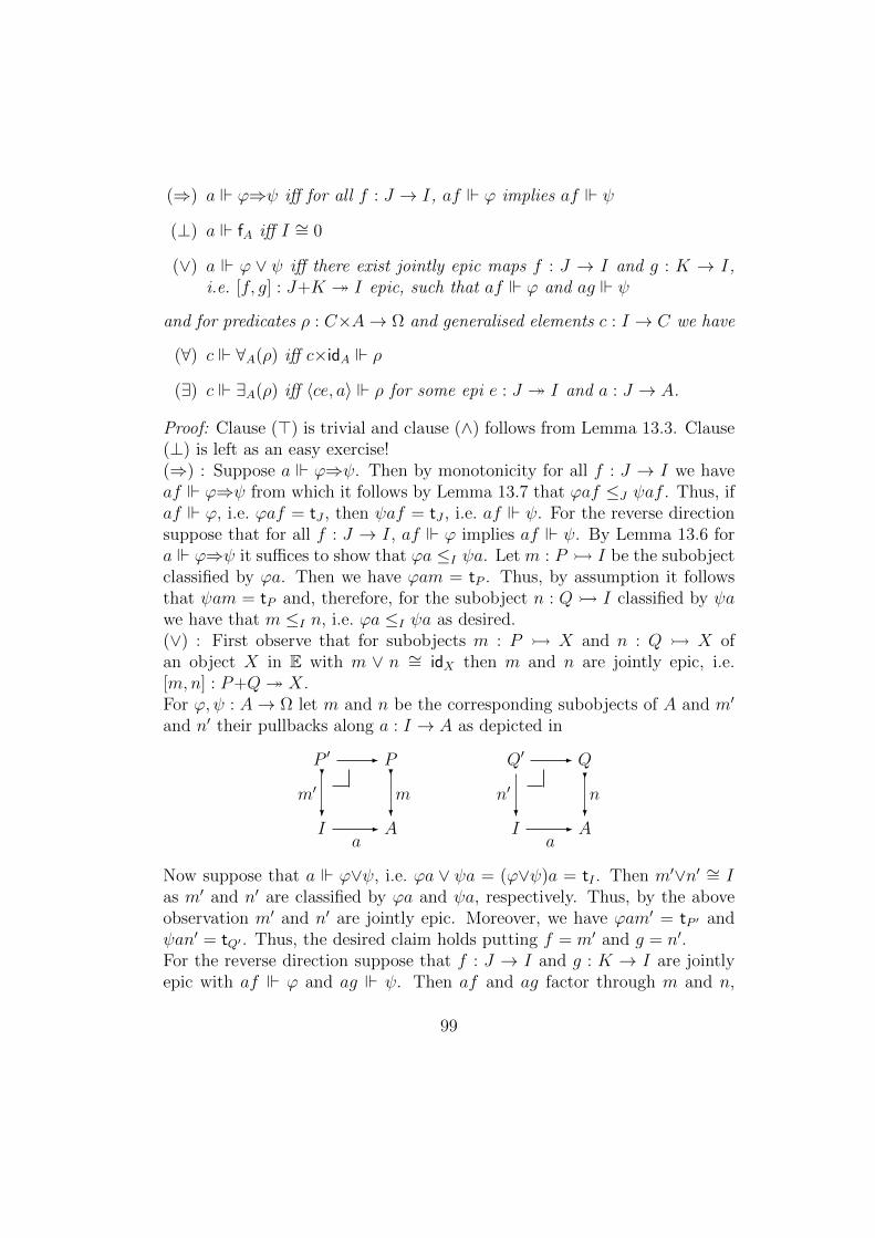
(⇒) a ϕ⇒ψ iff for all f : J → I, af ϕ implies af ψ

(⊥) a fA iff I ∼= 0

(∨) a ϕ ∨ ψ iff there exist jointly epic maps f : J → I and g : K → I,i.e. [f, g] : J+K I epic, such that af ϕ and ag ψ

and for predicates ρ : C×A→ Ω and generalised elements c : I → C we have

(∀) c ∀A(ρ) iff c×idA ρ

(∃) c ∃A(ρ) iff 〈ce, a〉 ρ for some epi e : J I and a : J → A.

Proof: Clause (>) is trivial and clause (∧) follows from Lemma 13.3. Clause(⊥) is left as an easy exercise!(⇒) : Suppose a ϕ⇒ψ. Then by monotonicity for all f : J → I we haveaf ϕ⇒ψ from which it follows by Lemma 13.7 that ϕaf ≤J ψaf . Thus, ifaf ϕ, i.e. ϕaf = tJ , then ψaf = tJ , i.e. af ψ. For the reverse directionsuppose that for all f : J → I, af ϕ implies af ψ. By Lemma 13.6 fora ϕ⇒ψ it suffices to show that ϕa ≤I ψa. Let m : P I be the subobjectclassified by ϕa. Then we have ϕam = tP . Thus, by assumption it followsthat ψam = tP and, therefore, for the subobject n : Q I classified by ψawe have that m ≤I n, i.e. ϕa ≤I ψa as desired.(∨) : First observe that for subobjects m : P X and n : Q X ofan object X in E with m ∨ n ∼= idX then m and n are jointly epic, i.e.[m,n] : P+Q X.For ϕ, ψ : A→ Ω let m and n be the corresponding subobjects of A and m′

and n′ their pullbacks along a : I → A as depicted in

P ′ - P Q′ - Q

I

m′

?

?

a- A

m?

?

I

n′

?

a- A

n?

?

Now suppose that a ϕ∨ψ, i.e. ϕa ∨ ψa = (ϕ∨ψ)a = tI . Then m′∨n′ ∼= Ias m′ and n′ are classified by ϕa and ψa, respectively. Thus, by the aboveobservation m′ and n′ are jointly epic. Moreover, we have ϕam′ = tP ′ andψan′ = tQ′ . Thus, the desired claim holds putting f = m′ and g = n′.For the reverse direction suppose that f : J → I and g : K → I are jointlyepic with af ϕ and ag ψ. Then af and ag factor through m and n,

99

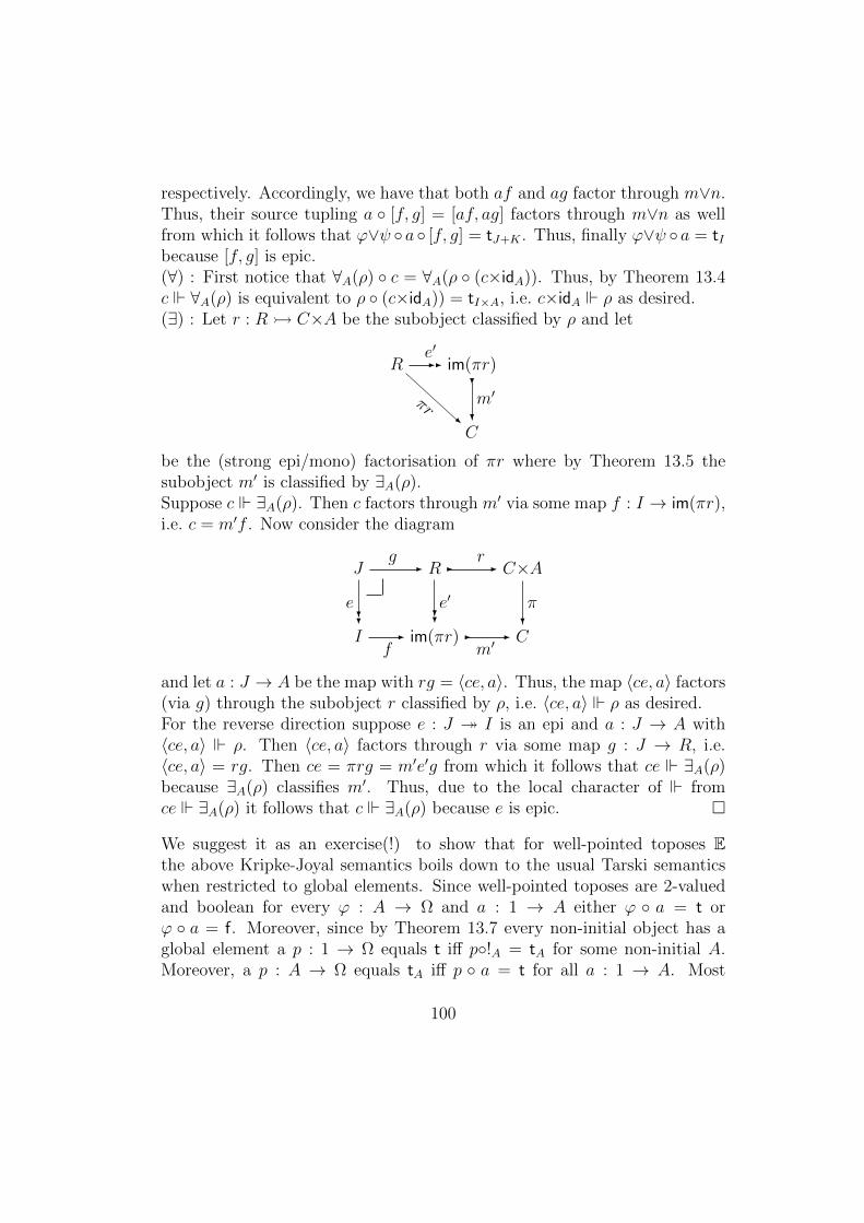
respectively. Accordingly, we have that both af and ag factor through m∨n.Thus, their source tupling a [f, g] = [af, ag] factors through m∨n as wellfrom which it follows that ϕ∨ψ a [f, g] = tJ+K . Thus, finally ϕ∨ψ a = tIbecause [f, g] is epic.(∀) : First notice that ∀A(ρ) c = ∀A(ρ (c×idA)). Thus, by Theorem 13.4c ∀A(ρ) is equivalent to ρ (c×idA)) = tI×A, i.e. c×idA ρ as desired.(∃) : Let r : R C×A be the subobject classified by ρ and let

Re′-- im(πr)

C

m′

?

?

πr -

be the (strong epi/mono) factorisation of πr where by Theorem 13.5 thesubobject m′ is classified by ∃A(ρ).Suppose c ∃A(ρ). Then c factors through m′ via some map f : I → im(πr),i.e. c = m′f . Now consider the diagram

Jg- R-

r- C×A

I

e??

f- im(πr)

e′??-m′- C

π?

and let a : J → A be the map with rg = 〈ce, a〉. Thus, the map 〈ce, a〉 factors(via g) through the subobject r classified by ρ, i.e. 〈ce, a〉 ρ as desired.For the reverse direction suppose e : J I is an epi and a : J → A with〈ce, a〉 ρ. Then 〈ce, a〉 factors through r via some map g : J → R, i.e.〈ce, a〉 = rg. Then ce = πrg = m′e′g from which it follows that ce ∃A(ρ)because ∃A(ρ) classifies m′. Thus, due to the local character of fromce ∃A(ρ) it follows that c ∃A(ρ) because e is epic.

We suggest it as an exercise(!) to show that for well-pointed toposes Ethe above Kripke-Joyal semantics boils down to the usual Tarski semanticswhen restricted to global elements. Since well-pointed toposes are 2-valuedand boolean for every ϕ : A → Ω and a : 1 → A either ϕ a = t orϕ a = f. Moreover, since by Theorem 13.7 every non-initial object has aglobal element a p : 1 → Ω equals t iff p!A = tA for some non-initial A.Moreover, a p : A → Ω equals tA iff p a = t for all a : 1 → A. Most

100

of the clauses of Theorem 13.7 translate straightforwardly. Only the casesof disjunction and existential quantification require a bit of thought. Forillustration we just discuss the case of existential quantification. Supposeρ : C × A → Ω then c ∃A(ρ) iff there exists a : I → A with !I : I → 1epic and ρ 〈c!I , a〉 = t. W.l.o.g. we may assume that I is not initial sinceotherwise 0 ∼= 1 and E is the trivial topos where all propositions are true.But by Lemma 12.2 the non-initial object I has a global element i : 1 → Iand thus ρ 〈c, ai〉 = > whenever ρ 〈c!I , a〉 = t. Thus c ∃A(ρ) iff thereexists a : 1→ A with 〈c, a〉 ρ.

In case of presheaf toposes Kripke-Joyal semantics takes the following evensimpler form based on the observation that a predicate ϕ : A → Ω is de-termined already by the set of generalized elements a : Y(I) → A withϕa = tY(I).

Theorem 13.8 (Kripke-Joyal semantics for presheaf toposes)

Let E be a presheaf topos C for some small category C. If A is an object of E,a ∈ A(I) and f : J → I is a morphism in C then we write af for A(f)(a)to make notation more readable. For predicates ϕ : A→ Ω and a ∈ A(I) wewrite I ϕ(a) iff a ∈ P (I) for the subpresheaf P → A classified by ϕ.Then for predicates ϕ, ψ : A→ Ω and a ∈ A(I) we have that

(>) I tA(a) always holds

(∧) I (ϕ∧ψ)(a) iff I ϕ(a) and I ψ(a)

(⇒) I (ϕ⇒ψ)(a) iff for all f : J → I, J ϕ(af) implies J ψ(af)

(⊥) I fA(a) never holds

(∨) I (ϕ∨ψ)(a) iff I ϕ(a) or I ψ(a)

and for predicates ρ : C×A→ Ω and c ∈ C(I) we have

(∀) I ∀A(ρ)(c) iff J ρ(cf, a) for all f : J → I in C and a ∈ A(J)

(∃) I ∃A(ρ)(c) iff I ρ(c, a) for some a ∈ A(I).

Proof: Exploiting the 1-1-correspondence between A(I) and morphism from

YC(I) to A in C as ensured by Yoneda most of the claims are immediate fromTheorem 13.7. For (⊥), (∨) and (∃) one has to exploit the specific nature of

101

presheaf toposes where 0(I) = ∅, (P∨Q)(I) = P (I)∪Q(I) and where a mape : A→ B is epic iff all eI : A(I)→ B(I) are surjective functions.Details are left to the reader as a straightforward exercise!

Axiom of Choice in Toposes

We have seen already that the axiom of unique choice holds in every topos.But what about

(AC) ∀R : P(B×A).(∀x:A.∃y:B.R(y, x))⇒∃f :BA.∀x:A.R(f(x), x)

the general axiom of choice in higher order logic?

Theorem 13.9 (Diaconescu)Every elementary topos validating (AC) is already boolean.

Proof: Let 0 and 1 be the two global elements of 2 = 1+1 as given by leftand right injection of 1 into 2. For ϕ ∈ Ω we define

Vi = x ∈ 2 | x=i ∨ ϕ ∈ P(2)

for i=0, 1. Thus it holds that ∀V ∈V0, V1.∃x∈2. x ∈ V . From this instanti-ating A by V0, V1 and B by 2 in (AC) it follows that

∃f ∈ 2V0,V1.∀V ∈V0, V1.f(V ) ∈ V

Thus, it holds that (f(V0) ∈ V0) ∧ (f(V1) ∈ V1), i.e. by definition of the Vithat (f(V0)=0 ∨ ϕ) ∧ (f(V1)=1 ∨ ϕ), from which it follows by distributivitythat

(f(V0)=0 ∧ f(V1)=1) ∨ ϕ

But the latter entails ϕ ∨ ¬ϕ which can be seen as follows. Of course, ϕentails ϕ∨¬ϕ. On the other hand f(V0)=0∧ f(V1)=1 implies ¬ϕ because ifϕ then V0 = V1 from which it follows that 0 = 1, a contradiction.

Thus, unrestricted choice entails classical logic but not33vice versa. See e.g.Chapter VI of [MM] for boolean toposes not validating AC.Validity of the logical scheme (AC) in a topos E is equivalent to the followingprinciple called Internal Axiom of Choice

33Notice that even the stronger theory ZF does not prove AC.

102

(IAC) If e is epic then eA is epic, too, for all objects A of E.

as shown on pp. 312-315 of [MM]. A stronger principle is the followingprinciple called External Axiom of Choice

(EAC) Every epimorphism e splits, i.e. there is a section s with e s = id.

Obviously, (EAC) entails (IAC) because every functor preserves split epi-morphism and thus, in particular, the functors (−)A do. Notice that for

nontrivial groups G in the presheaf topos G the unique map from the rep-resentable presheaf to 1 is a non-split epi because the representable presheafdoes not have any global element. We leave it as an exercise(!) (see e.g.[FS]) that a topos satisfies (EAC) if and only if it satisfies (IAC) and 1 isprojective, i.e. every A with A 1 has a global element.34 We leave it asan exercise(!) to show that a well-pointed topos satisfying (IAC) satisfies(EAC) as well.

Natural Numbers in Toposes

The category Setf of finite sets and maps between them is an example ofa well-pointed topos satisfying (EAC). Thus, in order to guarantee the ex-istence of some infinite type as e.g. the type of natural numbers we need afurther axiom.35

The following definition of natural numbers object (NNO) like many othernotions in this field goes back to F.W.Lawvere.

Definition 13.5 (Natural Numbers Object)A natural numbers object (NNO) in a category C with terminal object 1 isan object N in C together with morphisms z : 1→ N (zero) and s : N → N(successor) such that for every object A in C and morphisms a : 1→ A and

34Generally an object C in E is called projective (or a choice object) iff E(C,−) : E→ Setpreserves epimorphisms, i.e. for every epimorphism e : A B and every g : C → B thereexists an f : C → A with e f = g.

35Just as in ZFC which is modelled by the hereditary finite sets as long as one does notpostulate the infinity axiom.

103

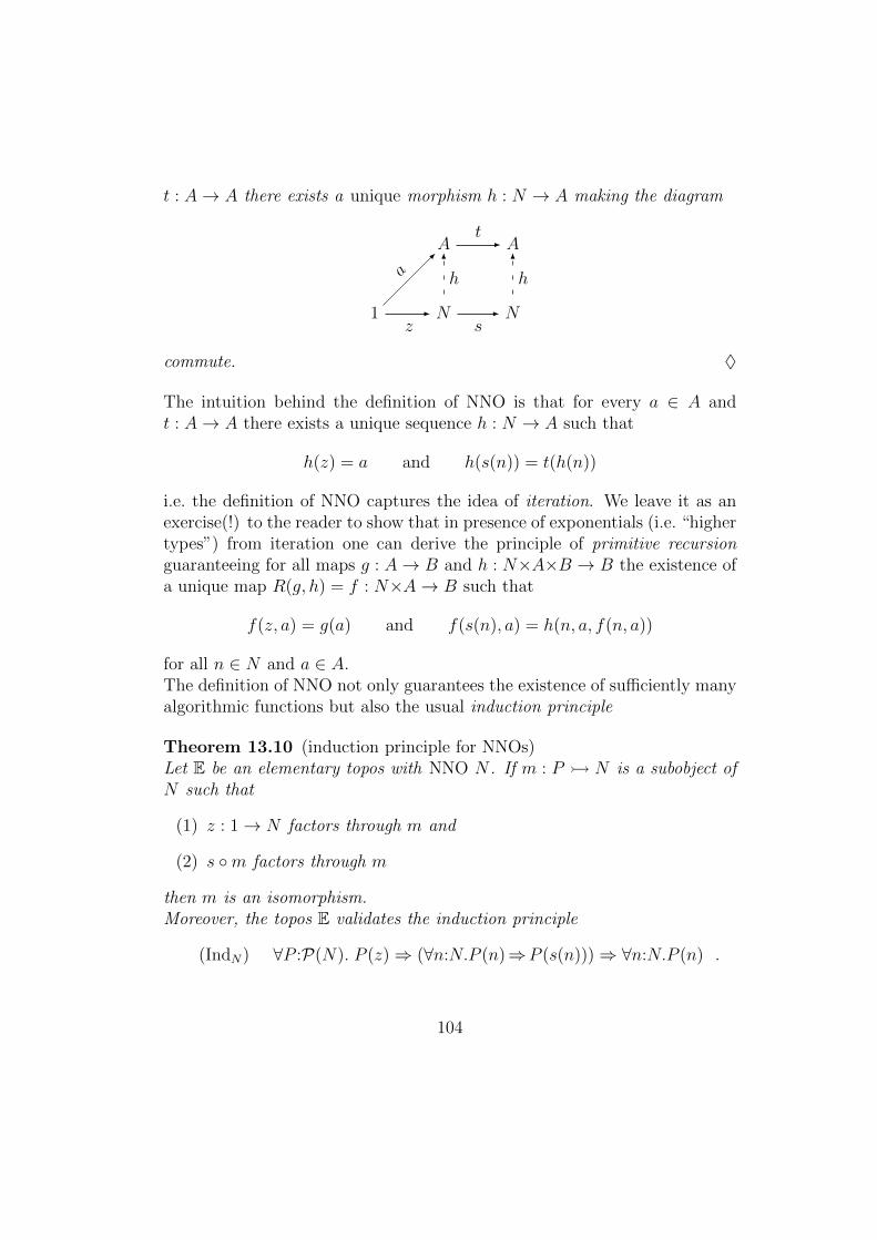
t : A→ A there exists a unique morphism h : N → A making the diagram

At- A

1z-

a-

N

h6

s- N

h6

commute. ♦

The intuition behind the definition of NNO is that for every a ∈ A andt : A→ A there exists a unique sequence h : N → A such that

h(z) = a and h(s(n)) = t(h(n))

i.e. the definition of NNO captures the idea of iteration. We leave it as anexercise(!) to the reader to show that in presence of exponentials (i.e. “highertypes”) from iteration one can derive the principle of primitive recursionguaranteeing for all maps g : A→ B and h : N×A×B → B the existence ofa unique map R(g, h) = f : N×A→ B such that

f(z, a) = g(a) and f(s(n), a) = h(n, a, f(n, a))

for all n ∈ N and a ∈ A.The definition of NNO not only guarantees the existence of sufficiently manyalgorithmic functions but also the usual induction principle

Theorem 13.10 (induction principle for NNOs)Let E be an elementary topos with NNO N . If m : P N is a subobject ofN such that

(1) z : 1→ N factors through m and

(2) s m factors through m

then m is an isomorphism.Moreover, the topos E validates the induction principle

(IndN) ∀P :P(N). P (z)⇒ (∀n:N.P (n)⇒P (s(n)))⇒ ∀n:N.P (n) .

104

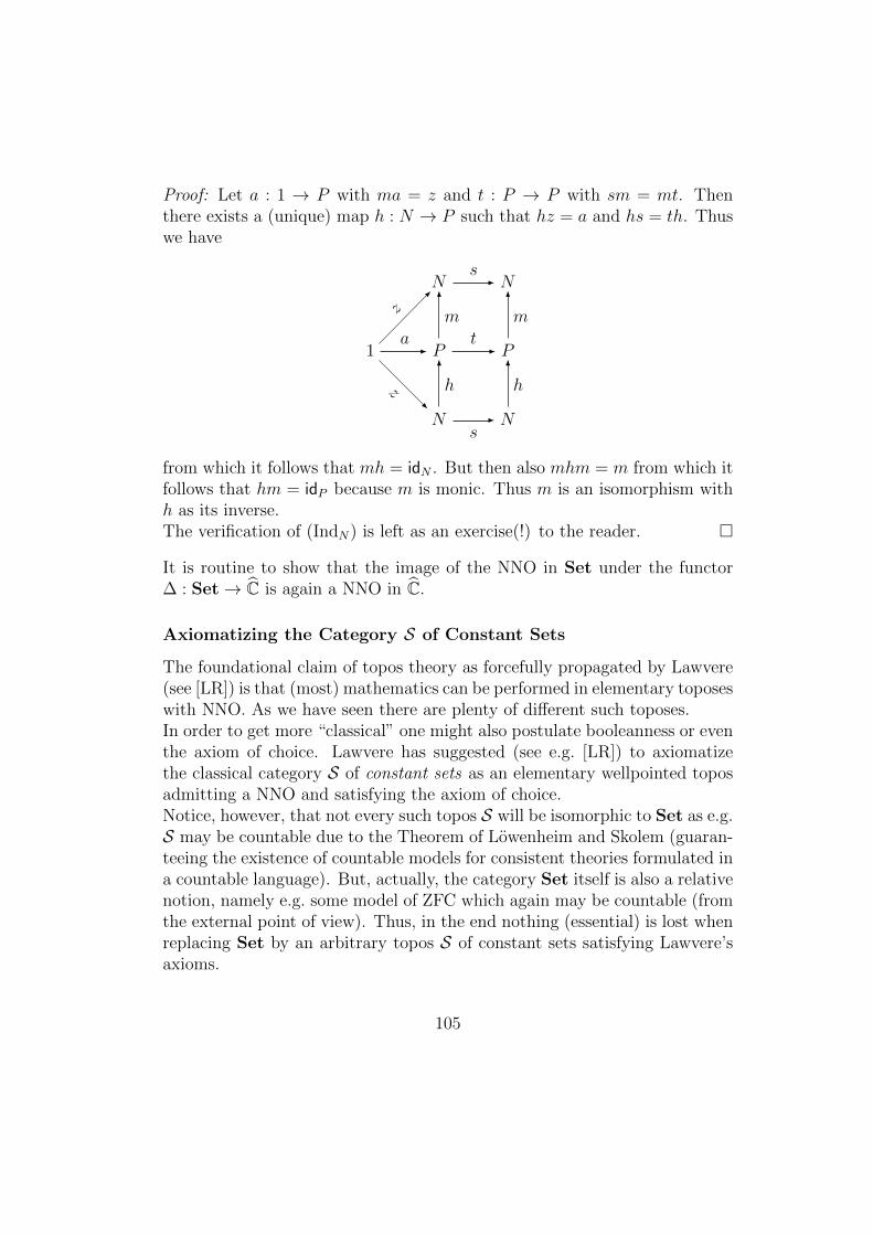
Proof: Let a : 1 → P with ma = z and t : P → P with sm = mt. Thenthere exists a (unique) map h : N → P such that hz = a and hs = th. Thuswe have

Ns- N

1a-

z-

P

m6

t- P

m6

N

h6

s-

z -

N

h6

from which it follows that mh = idN . But then also mhm = m from which itfollows that hm = idP because m is monic. Thus m is an isomorphism withh as its inverse.The verification of (IndN) is left as an exercise(!) to the reader.

It is routine to show that the image of the NNO in Set under the functor∆ : Set→ C is again a NNO in C.

Axiomatizing the Category S of Constant Sets

The foundational claim of topos theory as forcefully propagated by Lawvere(see [LR]) is that (most) mathematics can be performed in elementary toposeswith NNO. As we have seen there are plenty of different such toposes.In order to get more “classical” one might also postulate booleanness or eventhe axiom of choice. Lawvere has suggested (see e.g. [LR]) to axiomatizethe classical category S of constant sets as an elementary wellpointed toposadmitting a NNO and satisfying the axiom of choice.Notice, however, that not every such topos S will be isomorphic to Set as e.g.S may be countable due to the Theorem of Lowenheim and Skolem (guaran-teeing the existence of countable models for consistent theories formulated ina countable language). But, actually, the category Set itself is also a relativenotion, namely e.g. some model of ZFC which again may be countable (fromthe external point of view). Thus, in the end nothing (essential) is lost whenreplacing Set by an arbitrary topos S of constant sets satisfying Lawvere’saxioms.

105

14 Some Exercises in Presheaf Toposes

An excellent reference for examples of and computations in presheaf toposesis [PRZ] which we strongly recommend for this purpose.

A topos is called localic iff subobjects of 1 (called subterminals) generate inwhich case we say that the topos is localic.

Lemma 14.1 Let C be a small category. Then C is localic iff C is posetal.

Proof: Suppose C is posetal. Then all representable objects of C are subter-minal. Since representable objects generate it follows that C is localic.For the reverse direction suppose C is localic. We show that every repre-sentable object Y(I) is subterminal. For that purpose consider the subobjectS ⊆ Y(I) consisting of all u : J → I with uv1 = uv2 for all v1, v2 : K → J .Let χ : Y(I) → Ω be the classifying map for S. Suppose χ 6= >Y(I). Since

by assumption C is localic there exists a τ : U → Y(I) with U subterminaland χ τ 6= >U . Thus there exists a map v : J → I with χJ(v) 6= >J andvw1 = vw2 for all w1, w2 : K → J , i.e. v ∈ S(J) but χJ(v) 6= >J whichclearly is impossible since χ classifies S ⊆ Y(I). Thus we have shown thatχ = >Y(I) and, accordingly, we have S = Y(I) from which it follows thatidI ∈ S and therefore v1 = v2 whenever v1, v2 : J → I. Since this holds forall objects I of C it follows that C is indeed posetal.

Corollary 14.1 If for a small category C the topos C is localic and 2-valuedthen C ' 1 and thus C ' Set.

Proof: If C is localic then by the previous theorem C is posetal. If C werenot equivalent to the terminal category 1 then in C there would exist non-trivial subterminals corresponding to nontrivial global elements of Ω whichis impossible due to the assumption that C is 2-valued.

An alternative argument is the following one: if C is 2-valued then 0 and 1are the only subterminals from which it follows by the assumption of C beinglocalic that C is wellpointed which we have already seen to entail that C isequivalent to the terminal category.

Theorem 14.1 For a small category C the global sections functor Γ : C →Set has left adjoint ∆ which in turn has a further left adjoint π.

106

Proof: The left adjoint ∆ to Γ sends a set S to the constant presheaf withvalue S and f : S → T to the natural transformation ∆(f) with ∆(f)I = ffor all I ∈ C. The unit of ∆ a Γ at S sends x ∈ S to the global elementηS(x) : 1 → ∆(S) with (ηS(x))I(∗) = x. For f : S → Γ(A) the uniqueφ : ∆(S)→ A with Γ(φ) ηS = f is given by φI(x) = f(x)I(∗) ∈ A(I).The left adjoint π to ∆ sends a presheaf A to the set π(A) of connectedcomponents of Elts(A). The unit ηA : A → ∆(π(A)) sends a ∈ A to theconnected components inhabitated by a. Obviously, a natural transformationφ : A → ∆(S) is constant on connected components and, therefore, theunique f : π(A)→ S with ∆(f) ηS = φ sends a connected component of Ato the constant value of φ on it.

Theorem 14.2 Let C be a small category. Then Γ : C → Set has a rightadjoint ∇ iff the terminal object in C appears as retract of a representableobject.

Proof: If Γ has a right adjoint then Γ preserves colimits. Since 1 is a colimitof representable objects and Γ preserves colimits it follows that Γ(Y(I)) 6= ∅for some object I in C. Thus there exists e : 1→ Y(I) exhibiting 1 as retractof the representable object Y(I).Suppose 1 appears as retract of some Y(I). Then there exists e : 1 → Y(I).For every object J of C we have eJ : J → I and eJ u = eK for all u : K → Jin C. In particular, for eI we have eIeI = eI , i.e. eI is a retract. Next observethat Γ(A) ∼= a ∈ A(I) | A(eI)(a) = a by sending α : 1 → A to αI(∗).Conversely, given a ∈ A(I) with A(eI)(a) = a this induces an α : 1→ A withαJ(∗) = A(eJ)(a) for objects J in C. Moreover, for f : A→ B and a ∈ A(I)with A(eI)(a) = a we have B(e)(fI(a)) = fI(A(eI)(a)) = fI(a). Thus, upto isomorphism Γ looks as follows: Γ(A) = a ∈ A(I) | A(eI)(a) = aand Γ(f)(a) = fI(a). From now on we work with this isomorphic copy ofΓ. Define G : C → Set as G = Γ Y. More explicitly, we have G(J) =u : I → J | ueI = u and G(v)(u) = vu for v : J → K in C. Thenthe right adjoint to Γ is given by ∇(S) = SG(−). Its counit at S is givenby εS : Γ(∇(S)) → S : γ 7→ γ(eI). Suppose f : Γ(A) → S. We have toshow that there exists a unique φ : A → ∇(S) with εS Γ(φ) = f , i.e.

107

φI(a)(eI) = f(a) for a ∈ Γ(A). By naturality of φ we have for u ∈ G(J) that

A(J)φJ- SG(J)

A(I)

A(u)?

φI- SG(I)

SG(u)

?

and thus for a ∈ A(J) we have (since A(eI)(A(u)(a)) = A(ueI)(a) = A(u)(a)and thus A(u)(a) ∈ Γ(A)) that

φJ(a)(u) = φJ(G(u)(eI)) = SG(u)(φJ(a))(eI) == (SG(u) φJ)(a)(eI) = (φI A(u))(a)(eI) == φI(A(u)(a))(eI) =

= f(A(u)(a))

from which it follows that φ is determined uniquely f . Moreover, this obser-vation tells us how φ has to look like provided it exists, namely

φJ(a)(u) = f(A(u)(a))

for a ∈ A(J) and u ∈ G(J). It is a straightforward exercise to show that theso defined φ is actually natural. Moreover, for a ∈ Γ(A) we have

(εS Γ(φ))(a) = φI(a)(eI) = f(A(eI)(a)) = f(a)

and thus we have εS Γ(φ) = f as desired.

For the reverse implication of Theorem 14.2 we have the following alternativeProof: Suppose e0 : 1→ Y(I0). Let G = Γ Y : C→ Set. The right adjointto Γ is given by∇(S) = SG(−). The unit ηA : A→ ∇(Γ(A)) of the adjunctionΓ a ∇ at A is given by

(ηA)I(a)(i) = a i

for a : I → A and i : 1 → I. It is a straightforward exercise to show thatthe so defined η is actually natural. For showing that η is the unit of Γ ` ∇we have to show that for φ : A → ∇(S) there exists a unique f : Γ(A) → Swith ∇(f) ηA = φ, i.e.

φI(a)(i) =[∇(f) ηA

]I(a)(i) = f(a i)

108

for a : I → A and i : 1→ I. For α : 1→ A we may put a := α !I0 : I0 → Aand then have

f(α) = f(a e0) = φI0(a)(e0) = φI0(α !I0)(e0)

from which it follows that f is uniquely determined by φ. Now for a : I → Aand i : 1→ I we have[∇(f)ηA

]I(a)(i) = f(a i) = φI0(a i !I0)(e0) = φI(a)(i !I0 e0) = φI(a)(i)

and thus ∇(f) ηA = φ as desired.

Notice that in case Γ : C → Set has a right adjoint ∇ we have Γ∆ ∼= IdSet.From Lemma 8.1 it follows that the counit η : IdSet → Γ∆ is a naturalisomorphism and thus by Theorem 8.5 the functor ∆ is full and faithful.By uniqueness of adjoints from Γ∆ ∼= IdSet it follows that Γ∇ ∼= IdSet andthus by the dual versions of Lemma 8.1 and Theorem 8.5 that ∇ is alsofull and faithful and that εS : Γ(∇(S)) → S is an isomorphism for all S ∈Set. That’s what Lawvere calls a UIAO situation (for Unity and Identity ofAdjoint Opposites), i.e. L a F a R with F L = Id = F R where as abovefrom Lemma 8.1 it follows that both L and R are full and faithful.For the Sierpinski topos 2 the global sections functor is given by Γ(A) = A(1).Its right adjoint ∇ is given by ∇(S)(1) = S and ∇(S)(0) = ∗. The leftadjoint of Γ is given by ∆(S)(0→1) = idS. The left adjoint π of ∆ is given byπ(A) = A(0). The functor π has a further left adjoint given by L(S)(1) = ∅and L(S)(0) = S.Let Mn be the monoid whose elements besides the unit 1 are e0, . . . , en−1

with eiej = ei for 1 ≤ i, j < n.

The presheaf topos M1 consists of retractions and maps between them sincefor an object X of M1 the map rX(x) = x · e0 is a retraction (becauserX(rX(x)) = x · e0 · e0 = x · e0e0 = x · e0 = rX(x)) and for a morphismf : X → Y we have f(rX(x)) = f(x · e0) = f(x) · e0 = rY (f(x)). For X in

M1 we have Γ(X) = x ∈ X | rX(x) = x. For a set S let ∆(S) be the set Swith right action of M1 given by x · e0 = x for x ∈ S. One easily checks that∆ ` Γ ` ∆, i.e. that ∆ and ∇ coincide.36 Thus, also π coincides with Γ.The presheaf topos M2 may be considered as the topos of reflexive graphswhere for an object X of M2 the underlying set of X is thought of as the set

36The transpose of f : S → Γ(X) is the morphism f : ∆(S) → X and the transpose ofg : Γ(X)→ S is the morphism g : X → ∆(S) sending x ∈ X to g(x) = g(x · e0)

109

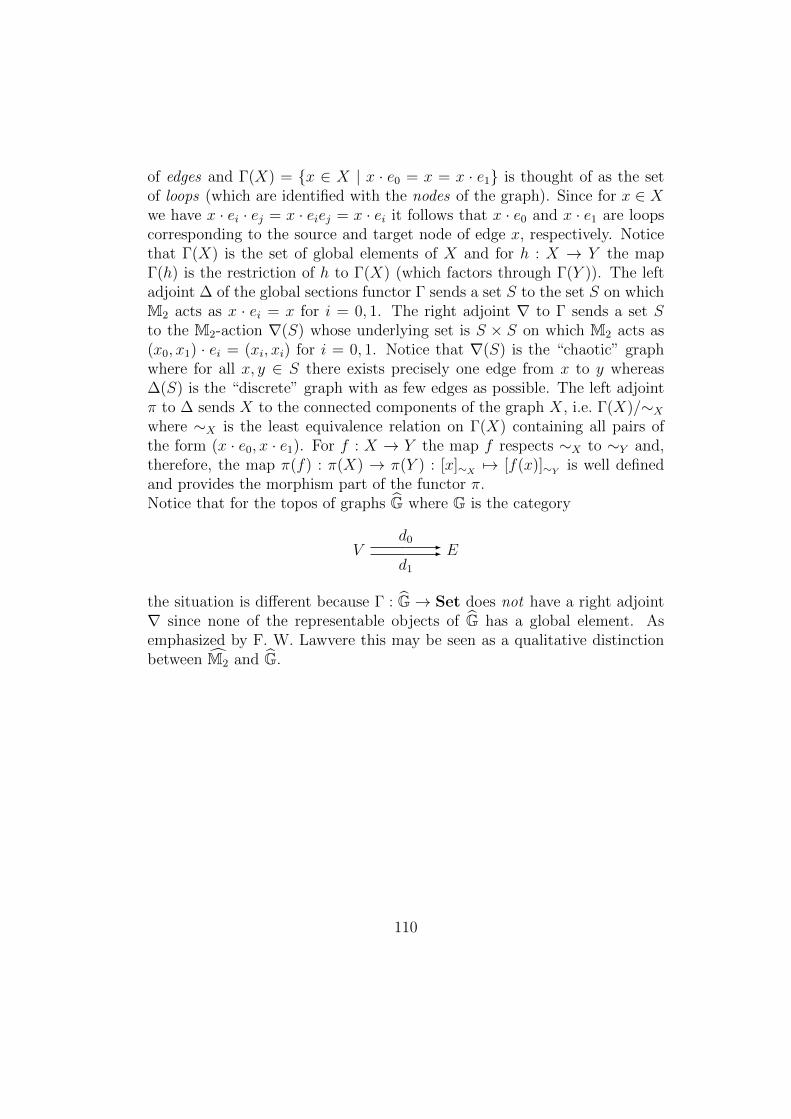
of edges and Γ(X) = x ∈ X | x · e0 = x = x · e1 is thought of as the setof loops (which are identified with the nodes of the graph). Since for x ∈ Xwe have x · ei · ej = x · eiej = x · ei it follows that x · e0 and x · e1 are loopscorresponding to the source and target node of edge x, respectively. Noticethat Γ(X) is the set of global elements of X and for h : X → Y the mapΓ(h) is the restriction of h to Γ(X) (which factors through Γ(Y )). The leftadjoint ∆ of the global sections functor Γ sends a set S to the set S on whichM2 acts as x · ei = x for i = 0, 1. The right adjoint ∇ to Γ sends a set Sto the M2-action ∇(S) whose underlying set is S × S on which M2 acts as(x0, x1) · ei = (xi, xi) for i = 0, 1. Notice that ∇(S) is the “chaotic” graphwhere for all x, y ∈ S there exists precisely one edge from x to y whereas∆(S) is the “discrete” graph with as few edges as possible. The left adjointπ to ∆ sends X to the connected components of the graph X, i.e. Γ(X)/∼Xwhere ∼X is the least equivalence relation on Γ(X) containing all pairs ofthe form (x · e0, x · e1). For f : X → Y the map f respects ∼X to ∼Y and,therefore, the map π(f) : π(X) → π(Y ) : [x]∼X

7→ [f(x)]∼Yis well defined

and provides the morphism part of the functor π.Notice that for the topos of graphs G where G is the category

Vd0 -

d1

- E

the situation is different because Γ : G→ Set does not have a right adjoint∇ since none of the representable objects of G has a global element. Asemphasized by F. W. Lawvere this may be seen as a qualitative distinctionbetween M2 and G.

110

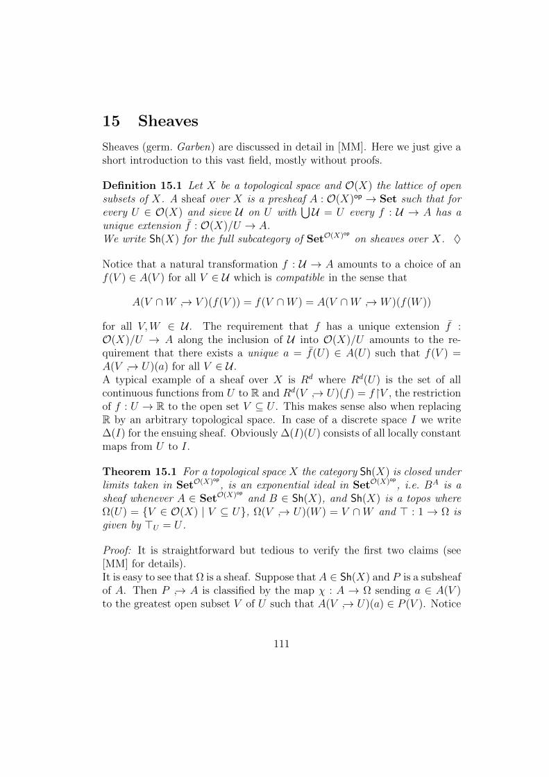
15 Sheaves

Sheaves (germ. Garben) are discussed in detail in [MM]. Here we just give ashort introduction to this vast field, mostly without proofs.

Definition 15.1 Let X be a topological space and O(X) the lattice of opensubsets of X. A sheaf over X is a presheaf A : O(X)op → Set such that forevery U ∈ O(X) and sieve U on U with

⋃U = U every f : U → A has a

unique extension f : O(X)/U → A.We write Sh(X) for the full subcategory of SetO(X)op on sheaves over X. ♦

Notice that a natural transformation f : U → A amounts to a choice of anf(V ) ∈ A(V ) for all V ∈ U which is compatible in the sense that

A(V ∩W → V )(f(V )) = f(V ∩W ) = A(V ∩W → W )(f(W ))

for all V,W ∈ U . The requirement that f has a unique extension f :O(X)/U → A along the inclusion of U into O(X)/U amounts to the re-quirement that there exists a unique a = f(U) ∈ A(U) such that f(V ) =A(V → U)(a) for all V ∈ U .A typical example of a sheaf over X is Rd where Rd(U) is the set of allcontinuous functions from U to R and Rd(V → U)(f) = fV , the restrictionof f : U → R to the open set V ⊆ U . This makes sense also when replacingR by an arbitrary topological space. In case of a discrete space I we write∆(I) for the ensuing sheaf. Obviously ∆(I)(U) consists of all locally constantmaps from U to I.

Theorem 15.1 For a topological space X the category Sh(X) is closed underlimits taken in SetO(X)op, is an exponential ideal in SetO(X)op, i.e. BA is asheaf whenever A ∈ SetO(X)op and B ∈ Sh(X), and Sh(X) is a topos whereΩ(U) = V ∈ O(X) | V ⊆ U, Ω(V → U)(W ) = V ∩W and > : 1 → Ω isgiven by >U = U .

Proof: It is straightforward but tedious to verify the first two claims (see[MM] for details).It is easy to see that Ω is a sheaf. Suppose that A ∈ Sh(X) and P is a subsheafof A. Then P → A is classified by the map χ : A → Ω sending a ∈ A(V )to the greatest open subset V of U such that A(V → U)(a) ∈ P (V ). Notice

111

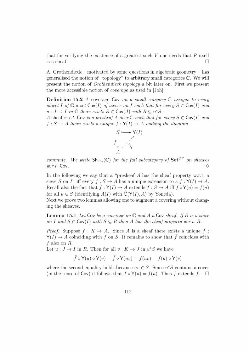
that for verifying the existence of a greatest such V one needs that P itselfis a sheaf.

A. Grothendieck – motivated by some questions in algebraic geometry – hasgeneralised the notion of “topology” to arbitrary small categories C. We willpresent the notion of Grothendieck topology a bit later on. First we presentthe more accessible notion of coverage as used in [Joh].

Definition 15.2 A coverage Cov on a small category C assigns to everyobject I of C a set Cov(I) of sieves on I such that for every S ∈ Cov(I) andu : J → I in C there exists R ∈ Cov(J) with R ⊆ u∗S.A sheaf w.r.t. Cov is a presheaf A over C such that for every S ∈ Cov(I) andf : S → A there exists a unique f : Y(I)→ A making the diagram

S ⊂ - Y(I)

A

f? f

-

commute. We write ShCov(C) for the full subcategory of SetCop

on sheavesw.r.t. Cov. ♦

In the following we say that a “presheaf A has the sheaf property w.r.t. asieve S on I” iff every f : S → A has a unique extension to a f : Y(I)→ A.Recall also the fact that f : Y(I)→ A extends f : S → A iff f Y(u) = f(u)

for all u ∈ S (identifying A(I) with C(Y(I), A) by Yoneda).Next we prove two lemmas allowing one to augment a covering without chang-ing the sheaves.

Lemma 15.1 Let Cov be a coverage on C and A a Cov-sheaf. If R is a sieveon I and S ∈ Cov(I) with S ⊆ R then A has the sheaf property w.r.t. R.

Proof: Suppose f : R → A. Since A is a sheaf there exists a unique f :Y(I)→ A coinciding with f on S. It remains to show that f coincides withf also on R.Let u : J → I in R. Then for all v : K → J in u∗S we have

f Y(u) Y(v) = f Y(uv) = f(uv) = f(u) Y(v)

where the second equality holds because uv ∈ S. Since u∗S contains a cover(in the sense of Cov) it follows that f Y(u) = f(u). Thus f extends f .

112

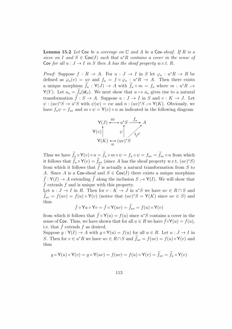
Lemma 15.2 Let Cov be a coverage on C and A be a Cov-sheaf. If R is asieve on I and S ∈ Cov(I) such that u∗R contains a cover in the sense ofCov for all u : J → I in S then A has the sheaf property w.r.t. R.

Proof: Suppose f : R → A. For u : J → I in S let ϕu : u∗R → R bedefined as ϕu(v) = uv and fu = f ϕu : u∗R → A. Then there exists

a unique morphism fu : Y(J) → A with fu m = fu where m : u∗R →Y(Y ). Let au = fu(idJ). We next show that u 7→ au gives rise to a natural

transformation f : S → A. Suppose u : J → I in S and v : K → J . Letψ : (uv)∗S → u∗S with ψ(w) = vw and n : (uv)∗S → Y(K). Obviously, wehave fuψ = fuv and m ψ = Y(v) n as indicated in the following diagram

Y(J) mu∗S

fu- A

Y(K)

Y(v)6

n(uv)∗S

ψ6

f uv

-

Thus we have fu Y(v) n = fu m ψ = fu ψ = fuv = fuv n from which

it follows that fu Y(v) = fuv (since A has the sheaf property w.r.t. (uv)∗S)

from which it follows that f is actually a natural transformation from S toA. Since A is a Cov-sheaf and S ∈ Cov(I) there exists a unique morphism

f : Y(I)→ A extending f along the inclusion S → Y(I). We will show thatf extends f and is unique with this property.Let u : J → I in R. Then for v : K → J in u∗S we have uv ∈ R ∩ S andfuv = f(uv) = f(u) Y(v) (notice that (uv)∗S = Y(K) since uv ∈ S) andthus

f Yu Yv = f Y(uv) = fuv = f(u) Y(v)

from which it follows that f Y(u) = f(u) since u∗S contains a cover in thesense of Cov. Thus, we have shown that for all u ∈ R we have f Y(u) = f(u),i.e. that f extends f as desired.Suppose g : Y(I) → A with g Y(u) = f(u) for all u ∈ R. Let u : J → I in

S. Then for v ∈ u∗R we have uv ∈ R∩S and fuv = f(uv) = f(u) Y(v) andthus

g Y(u) Y(v) = g Y(uv) = f(uv) = f(u) Y(v) = fuv = fu Y(v)

113

from which it follows that g Y(u) = fu since by assumption u∗R contains acover in the sense of Cov. Thus, we have shown that for all u ∈ S we haveg Y(u) = fu = f(u) from which it follows that g = f since S ∈ Cov(I) andA is a Cov-sheaf. Thus we have shown uniqueness of f .

We have the following analogue of Theorem 15.1

Theorem 15.2 Let Cov be a coverage on a small category C. Then ShCov(C)is closed under limits taken in SetC

op

, is an exponential ideal in SetCop

, i.e.BA is a sheaf whenever A ∈ SetC

op

and B ∈ ShCov(C), and ShCov(C) is atopos.The subobject classifier Ω for ShCov(C) can be described as follows. For I ∈C, Ω(I) consists of all Cov-closed sieves on I, i.e. sieves S on I such thatu : J → I is in S whenever u∗S ∈ Cov(J), Ω(u)(S) = u∗S and >I = >I .

Proof: It is straightforward but tedious to verify the first two claims (see[MM] for details).It is easy to see that Ω is a sheaf. Suppose that A ∈ ShCov(C) and P is a sheafof A. Then P → A is classified by the map χ : A→ Ω sending a ∈ A(V ) tothe sieve χI(a) = u : J → I | A(u)(a) ∈ P (J). Notice that for verifyingthat χI(a) is closed one needs that P itself is a sheaf.

A coverage Cov on C can be saturated to a so-called Grothendieck topologyon C which notion we define next.

Definition 15.3 A Grothendieck topology on a small category C is a cov-erage J with >I ∈ J (I) for all I ∈ C and satisfying the following localityproperty

(L) if R is a sieve on I and S ∈ J (I) with u∗R ∈ J (J) for all u : J → Iin S then R ∈ J (I). ♦

Notice that the locality property entails that J (I) is upward closed withinsieves on I.Obviously, Grothendieck topologies on C are closed under (componentwise)intersections. Thus, for every coverage Cov there exists a least Grothendiecktopology J on C with Cov ⊆ J . Notice that this way J is obtained fromCov by an inductive definition which in general stabilizes at a very transfiniteordinal.The next lemma says that sheaves w.r.t. Cov and sheaves w.r.t. the inducedJ coincide.

114

Lemma 15.3 Let J be the least Grothendieck topology containing Cov. Thena presheaf A ∈ SetC

op

is a Cov-sheaf iff it is a J -sheaf.

Proof: Obviously, since Cov ⊆ J every J -sheaf is also a Cov-sheaf.For the reverse inclusion it suffices to show that the collection JA of all sievesS on some I such that for all u : J → I, A satisfies the sheaf condition w.r.t.u∗S forms a Grothendieck topology. Obviously JA is a coverage containingall maximal sieves >I . So it remains to show that JA satisfies the localityproperty (L). Suppose R is a sieve on I and S ∈ JA(I) with u∗R ∈ JA(J) forall u : J → I in S. We have to show that R ∈ JA(I), i.e. that A has the sheafproperty w.r.t. to all reindexings of R. Let u : J → I. Then u∗S ∈ JA(J)and for all v : K → J in u∗S we have v∗u∗R = (uv)∗R ∈ JA(K) since uv ∈ S.Thus by Lemma 15.2 the presheaf A satisfies the sheaf condition w.r.t. u∗Ras desired.

One can show that a subobject J of Ω in C is a Grothendieck topology ifand only if the classifying map j : Ω→ Ω for J → Ω satisfies the conditions

(j1) j > = >

(j2) j ∧ = ∧ (j × j)

(j3) j j = j.

In an arbitrary topos E it makes sense to consider maps j : Ω→ Ω satisfyingthe conditions (j1)-(j3). Such maps are called Lawvere-Tierney toplogies ontopos E. A mono m : P X in E is called j-dense iff its characteristicmap χ : A → Ω satisfies j χ = >A. One then defines an object A of E tobe a j-sheaf iff E(m,A) : E(X,A) → E(P,A) is a bijection for all j-densemonos m in E. One can show that the full subcategory Ej of E on j-sheavesis a topos and that the inclusion i : Ej → E has a finite limit preserving leftadjoint a called sheafification. Moreover, if j is the characteristic map for aGrothendieck topology J on C then Cj coincides with ShJ (C). Accordingly,

the inclusion of ShJ (C) into C has a finite limit preserving left adjoint (alsocalled sheafification.By definition a Grothendieck topos is a topos equivalent to one of the formShJ (C) where J is a Grothendieck topology on a small category C.Grothendieck toposes can be characterized more abstractly as follows.

Theorem 15.3 E is a Grothendieck topos iff E is a locally small elementarytopos with small sums and a small generating family.

115

Proof: See e.g. [MM].

For Grothendieck toposes ShJ (C) one can give a Kripke-Joyal semanticswhich differs from the one for SetC

op

only for ⊥, ∨ and ∃, namely as follows

(⊥) I ⊥ iff ∅ ∈ J (I)

(∨) I (φ∨ψ)(a) iff there exists a J -covering family (uj : Ij → I)j∈J suchthat for all j ∈ J , Ij φ(auj) or Ij ψ(auj)

(∃) I ∃x:A.ρ(x, c) iff there exists a J -covering family (uj : Ij → I)j∈Jand a family

(aj ∈ A(Ij)

)j∈J such that Ij ρ(aj, cuj) for all j ∈ J

where (uj : Ij → I)j∈J is J -covering iff the induced sieve on I is in J (I).Thus, for disjunctions and existential statements it is easier to be valid inShJ (C) than in SetC

op

because it suffices for them to hold only “locally” andthey need not necessarily hold “globally”.

116