Draft version April 27, 2018 ABSTRACT arXiv:1804.10047v1 ...
15
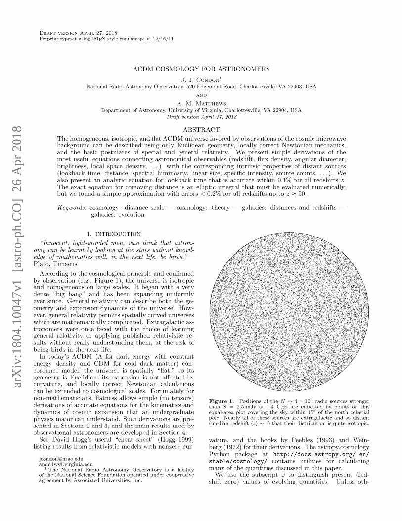
Draft version April 27, 2018 Preprint typeset using L A T E X style emulateapj v. 12/16/11 ΛCDM COSMOLOGY FOR ASTRONOMERS J. J. Condon 1 National Radio Astronomy Observatory, 520 Edgemont Road, Charlottesville, VA 22903, USA and A. M. Matthews Department of Astronomy, University of Virginia, Charlottesville, VA 22904, USA Draft version April 27, 2018 ABSTRACT The homogeneous, isotropic, and flat ΛCDM universe favored by observations of the cosmic microwave background can be described using only Euclidean geometry, locally correct Newtonian mechanics, and the basic postulates of special and general relativity. We present simple derivations of the most useful equations connecting astronomical observables (redshift, flux density, angular diameter, brightness, local space density, . . . ) with the corresponding intrinsic properties of distant sources (lookback time, distance, spectral luminosity, linear size, specific intensity, source counts, . . . ). We also present an analytic equation for lookback time that is accurate within 0.1% for all redshifts z. The exact equation for comoving distance is an elliptic integral that must be evaluated numerically, but we found a simple approximation with errors < 0.2% for all redshifts up to z ≈ 50. Keywords: cosmology: distance scale — cosmology: theory — galaxies: distances and redshifts — galaxies: evolution 1. INTRODUCTION “Innocent, light-minded men, who think that astron- omy can be learnt by looking at the stars without knowl- edge of mathematics will, in the next life, be birds.”— Plato, Timaeus According to the cosmological principle and confirmed by observation (e.g., Figure 1), the universe is isotropic and homogeneous on large scales. It began with a very dense “big bang” and has been expanding uniformly ever since. General relativity can describe both the ge- ometry and expansion dynamics of the universe. How- ever, general relativity permits spatially curved universes which are mathematically complicated. Extragalactic as- tronomers were once faced with the choice of learning general relativity or applying published relativistic re- sults without really understanding them, at the risk of being birds in the next life. In today’s ΛCDM (Λ for dark energy with constant energy density and CDM for cold dark matter) con- cordance model, the universe is spatially “flat,” so its geometry is Euclidian, its expansion is not affected by curvature, and locally correct Newtonian calculations can be extended to cosmological scales. Fortunately for non-mathematicians, flatness allows simple (no tensors) derivations of accurate equations for the kinematics and dynamics of cosmic expansion that an undergraduate physics major can understand. Such derivations are pre- sented in Sections 2 and 3, and the main results used by observational astronomers are developed in Section 4. See David Hogg’s useful “cheat sheet” (Hogg 1999) listing results from relativistic models with nonzero cur- [email protected] [email protected] 1 The National Radio Astronomy Observatory is a facility of the National Science Foundation operated under cooperative agreement by Associated Universities, Inc. Figure 1. Positions of the N ∼ 4 × 10 4 radio sources stronger than S =2.5 mJy at 1.4 GHz are indicated by points on this equal-area plot covering the sky within 15 ◦ of the north celestial pole. Nearly all of these sources are extragalactic and so distant (median redshift hzi∼ 1) that their distribution is quite isotropic. vature, and the books by Peebles (1993) and Wein- berg (1972) for their derivations. The astropy.cosmology Python package at http://docs.astropy.org/ en/ stable/cosmology/ contains utilities for calculating many of the quantities discussed in this paper. We use the subscript 0 to distinguish present (red- shift zero) values of evolving quantities. Unless oth- arXiv:1804.10047v1 [astro-ph.CO] 26 Apr 2018
Transcript of Draft version April 27, 2018 ABSTRACT arXiv:1804.10047v1 ...
Draft version April 27, 2018Preprint typeset using LATEX style emulateapj v. 12/16/11
ΛCDM COSMOLOGY FOR ASTRONOMERS
J. J. Condon1
National Radio Astronomy Observatory, 520 Edgemont Road, Charlottesville, VA 22903, USA
and
A. M. MatthewsDepartment of Astronomy, University of Virginia, Charlottesville, VA 22904, USA
Draft version April 27, 2018
ABSTRACT
The homogeneous, isotropic, and flat ΛCDM universe favored by observations of the cosmic microwavebackground can be described using only Euclidean geometry, locally correct Newtonian mechanics,and the basic postulates of special and general relativity. We present simple derivations of themost useful equations connecting astronomical observables (redshift, flux density, angular diameter,brightness, local space density, . . . ) with the corresponding intrinsic properties of distant sources(lookback time, distance, spectral luminosity, linear size, specific intensity, source counts, . . . ). Wealso present an analytic equation for lookback time that is accurate within 0.1% for all redshifts z.The exact equation for comoving distance is an elliptic integral that must be evaluated numerically,but we found a simple approximation with errors < 0.2% for all redshifts up to z ≈ 50.
Keywords: cosmology: distance scale — cosmology: theory — galaxies: distances and redshifts —galaxies: evolution
1. INTRODUCTION
“Innocent, light-minded men, who think that astron-omy can be learnt by looking at the stars without knowl-edge of mathematics will, in the next life, be birds.”—Plato, Timaeus
According to the cosmological principle and confirmedby observation (e.g., Figure 1), the universe is isotropicand homogeneous on large scales. It began with a verydense “big bang” and has been expanding uniformlyever since. General relativity can describe both the ge-ometry and expansion dynamics of the universe. How-ever, general relativity permits spatially curved universeswhich are mathematically complicated. Extragalactic as-tronomers were once faced with the choice of learninggeneral relativity or applying published relativistic re-sults without really understanding them, at the risk ofbeing birds in the next life.
In today’s ΛCDM (Λ for dark energy with constantenergy density and CDM for cold dark matter) con-cordance model, the universe is spatially “flat,” so itsgeometry is Euclidian, its expansion is not affected bycurvature, and locally correct Newtonian calculationscan be extended to cosmological scales. Fortunately fornon-mathematicians, flatness allows simple (no tensors)derivations of accurate equations for the kinematics anddynamics of cosmic expansion that an undergraduatephysics major can understand. Such derivations are pre-sented in Sections 2 and 3, and the main results used byobservational astronomers are developed in Section 4.
See David Hogg’s useful “cheat sheet” (Hogg 1999)listing results from relativistic models with nonzero cur-
[email protected]@virginia.edu
1 The National Radio Astronomy Observatory is a facilityof the National Science Foundation operated under cooperativeagreement by Associated Universities, Inc.
Figure 1. Positions of the N ∼ 4 × 10⁴ radio sources strongerthan S = 2.5 mJy at 1.4 GHz are indicated by points on thisequal-area plot covering the sky within 15 of the north celestialpole. Nearly all of these sources are extragalactic and so distant(median redshift 〈z〉 ∼ 1) that their distribution is quite isotropic.
vature, and the books by Peebles (1993) and Wein-berg (1972) for their derivations. The astropy.cosmologyPython package at http://docs.astropy.org/ en/stable/cosmology/ contains utilities for calculatingmany of the quantities discussed in this paper.
We use the subscript 0 to distinguish present (red-shift zero) values of evolving quantities. Unless oth-
arX
iv:1
804.
1004
7v1
[as
tro-
ph.C
O]
26
Apr
201
8
2 Condon & Matthews
erwise noted, all numerical results are based on aHubble constant H0 = 70 km s−1 Mpc−1 so h ≡H0/(100 km s−1 Mpc−1) = 0.7, plus the following nor-malized densities at redshift zero: total Ω0 = 1, bary-onic and cold dark matter Ω0,m = 0.3, radiation andrelic neutrinos Ω0,r = h−2 · 4.2 × 10−5, and dark energyΩ0,Λ = 1− (Ω0,m + Ω0,r) ≈ 0.7. Note that many authorsjust write Ω, Ωm, Ωr, and ΩΛ without the subscript 0to indicate the present values of these densities. Also,1 Mpc ≈ 3.0857× 10¹⁹ km and 1 yr ≈ 3.1557× 10⁷ s.
2. EXPANSION KINEMATICS
According to the equivalence principle, all fundamen-tal observers locally at rest relative to their surround-ings anywhere in the isotropically expanding (and hencehomogeneous) universe are in inertial frames, and theirclocks all agree on the time t elapsed since the big bang.This universal time t is sometimes called world time orcosmic time, and it equals the proper time of all funda-mental observers. Fundamental observers didn’t have tobe present at the creation to synchronize their clocks; thetemperature of the cosmic microwave background (CMB)radiation is a suitable proxy for time. Likewise, theCMB appears isotropic only to fundamental observers,and others can use the CMB dipole anisotropy (Kogutet al. 1993) to deduce their usually small (v2 c2, wherec ≈ 299792 km s−1 is the vacuum speed of light) peculiarvelocities and correct for them if necessary.
Homogeneity and isotropy are preserved if and only ifthe small proper distance D(t) between any close pair ofobservers expands as
D(t) = a(t)D0 , (1)
where D0 is the proper distance now and a(t) is the uni-versal (meaning, it is the same at every position in theuniverse) dimensionless scale factor that grew with timefrom a ≈ 0 just after the big bang to a(t0) ≡ 1 today(Figure 2). Equation 1 applies to any expansion thatpreserves homogeneity and isotropy—the separations ofdots on a photo being enlarged, for example. The cos-mological expansion affects only to the separations ofnon-interacting objects, and the dots representing rigidrulers, gravitationally bound galaxies, etc. do not ex-pand with the universe.
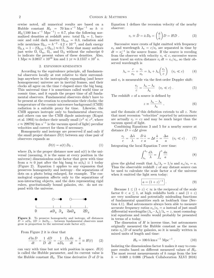
Figure 2. To preserve homogeneity and isotropy, all distancesD = aD0, 2D = 2aD0,. . . between fundamental observers mustgrow in proportion to the universal scale factor a(t).
From Figure 2 it is clear that
d lnD
dt=
1
D
dD
dt=
1
aD0
D0 da
dt=a
a≡ H(t) (2)
can vary with time but not with position in space. H(t)is called the Hubble parameter, and its current value isthe Hubble constant H0. The time derivative D of D in
Equation 1 defines the recession velocity of the nearbyobserver:
vr ≡ D = a D0 =
(a
a
)D = HD . (3)
Successive wave crests of light emitted with frequencyνe and wavelength λe = c/νe are separated in time bydt = ν−1
e in the source frame. If the source is recedingfrom the observer with velocity vr c, successive wavesmust travel an extra distance vr dt = vr/νe, so their ob-served wavelength is
λo =c
νe+vr
νe= λe + λe
(vr
c
)(vr c) (4)
and vr is measurable via the first-order Doppler shift:
vr
c=λo − λe
λe(vr c) . (5)
The redshift z of a source is defined by
z ≡ λo − λe
λe, (6)
and the domain of this definition extends to all z. Notethat most recession “velocities” reported by astronomersare actually vr = cz and may be much larger than thevacuum speed of light.
Combining Equations 3 and 5 for a nearby source atdistance D = c∆t gives
vr
c=
∆λ
λ=D
c
a
a= ∆t
a
a=
∆a
a(vr c) . (7)
Integrating the local Equation 7 over time:∫ λo
λe
dλ
λ=
∫ 1
a
da
a(8)
gives the global result that λo/λe = 1/a and νo/νe = a.Thus the observable redshift z of any distant source canbe used to calculate the scale factor a of the universewhen it emitted the light seen today:
a = (1 + z)−1 . (9)
Because 1 ≤ (1 + z) <∞ is the reciprocal of the scalefactor 0 < a ≤ 1, at high redshifts both z and (1 + z)are very nonlinear and potentially misleading functionsof fundamental quantities such as lookback time (Sec-tion 4.1). Had astronomers always been able to measureaccurate frequency ratios νo/νe = a instead of just smalldifferential wavelengths (λo−λe)/λe = z, most cosmolog-ical equations and results would probably be presentedin terms of a today.
The dimension of H is inverse time, but astronomersoriginally measured the Hubble constant as the meanratio vr/D of nearby galaxies, so it is usually written inmixed units of length and time:
H0 = 100h km s−1 Mpc−1 . (10)
Isolating the dimensionless factor h makes it easy to com-pare results based on different measured values of H0.The most recent measurements of h range from the lowh = 0.669 ± 0.006 (Planck Collaboration XLVI 2016)
ΛCDM Cosmology for Astronomers 3
derived by comparing the observed angular power spec-trum of CMB fluctuations with a flat ΛCDM cosmolog-ical model to the high h = 0.732 ± 0.017 (Riess et al.2016) based on relatively local measurements of Cepheidvariable stars and Type Ia supernovae used as standardcandles. The 3σ “tension” between these results is atopic of current research (Freedman 2017).
The Hubble time is defined by
tH ≡ H−1 , (11)
and its present value
tH0 ≡ H−10 ≈ 9.778× 10⁹ h−1 yr ≈ 14.0 Gyr (12)
is a convenient unit of time comparable with the presentage of the universe t0. Likewise, the current Hubble dis-tance
DH0≡ c
H0≈ 2998h−1 Mpc ≈ 4280 Mpc (13)
is a distance comparable with the present radius of theobservable universe.
The lookback time tL(z) to a source at any redshift zis the time photons needed to travel with speed c fromthe source to the observer at z = 0. In a homogeneousuniverse, this global quantitity is just the sum of thesmall locally measured proper times dt. In terms of thescale factor a and H = d ln(a)/dt, it is
tL =
∫ t0
t
dt′ =
∫ 1
a
(dt′
d ln(a′)
)d ln(a′) (14)
tL =
∫ 1
a
da′
a′H(a′). (15)
The lookback time is usually written in terms of z:
tL =
∫ t0
t
dt′ =
∫ 0
z
(dt′
dz′
)dz′ . (16)
To calculate dt/dz, take the time derivative of Equa-tion 9:
dz
dt=−1
a2
da
dt= −1
a
(a
a
)= −(1 + z)H (17)
so
tL =
∫ z
0
dz′
(1 + z′)H(z′). (18)
The dynamical equation specifying the evolution of H isderived in Section 3.
3. EXPANSION DYNAMICS
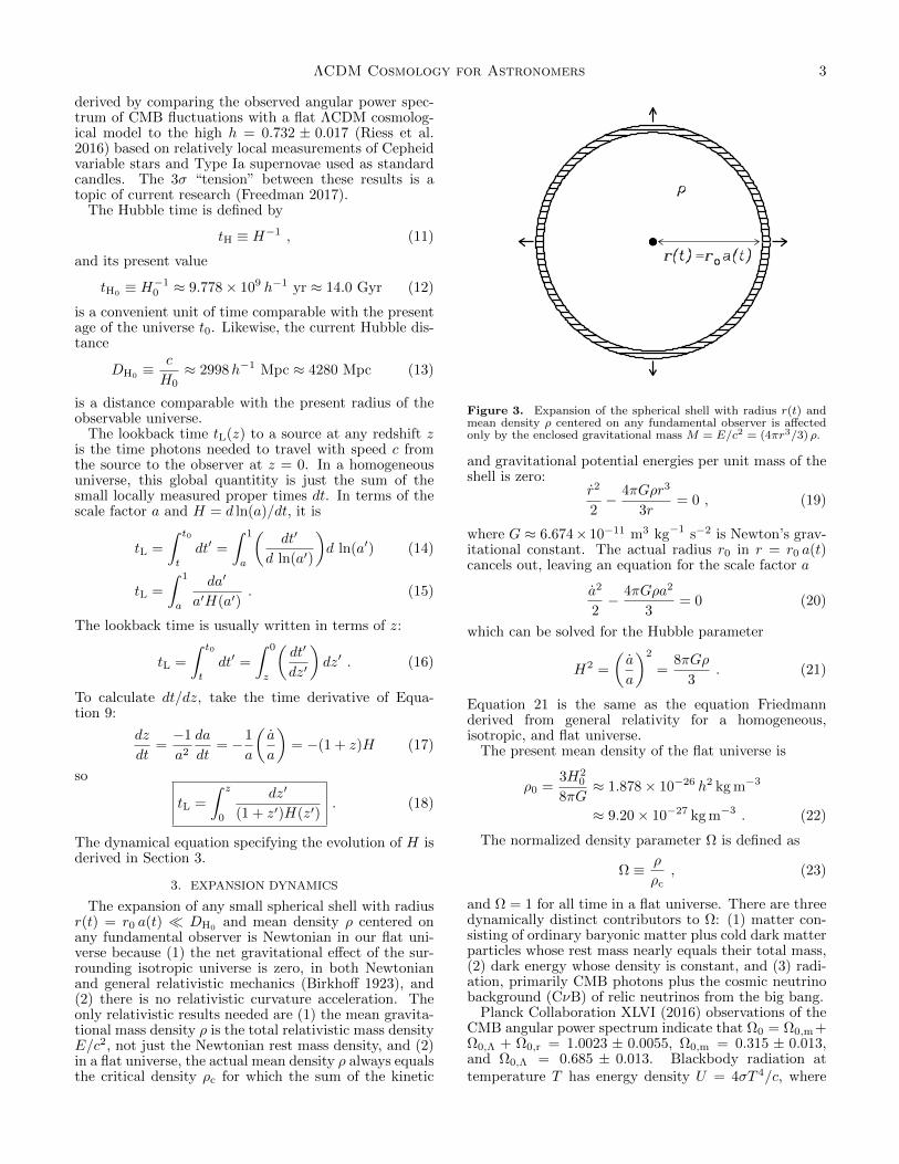
The expansion of any small spherical shell with radiusr(t) = r0 a(t) DH0
and mean density ρ centered onany fundamental observer is Newtonian in our flat uni-verse because (1) the net gravitational effect of the sur-rounding isotropic universe is zero, in both Newtonianand general relativistic mechanics (Birkhoff 1923), and(2) there is no relativistic curvature acceleration. Theonly relativistic results needed are (1) the mean gravita-tional mass density ρ is the total relativistic mass densityE/c2, not just the Newtonian rest mass density, and (2)in a flat universe, the actual mean density ρ always equalsthe critical density ρc for which the sum of the kinetic
Figure 3. Expansion of the spherical shell with radius r(t) andmean density ρ centered on any fundamental observer is affectedonly by the enclosed gravitational mass M = E/c2 = (4πr3/3) ρ.
and gravitational potential energies per unit mass of theshell is zero:
r2
2− 4πGρr3
3r= 0 , (19)
where G ≈ 6.674× 10⁻¹¹ m3 kg−1 s−2 is Newton’s grav-itational constant. The actual radius r0 in r = r0 a(t)cancels out, leaving an equation for the scale factor a
a2
2− 4πGρa2
3= 0 (20)
which can be solved for the Hubble parameter
H2 =
(a
a
)2
=8πGρ
3. (21)
Equation 21 is the same as the equation Friedmannderived from general relativity for a homogeneous,isotropic, and flat universe.
The present mean density of the flat universe is
ρ0 =3H2
0
8πG≈ 1.878× 10⁻²⁶ h2 kg m−3
≈ 9.20× 10⁻²⁷ kg m−3 . (22)
The normalized density parameter Ω is defined as
Ω ≡ ρ
ρc, (23)
and Ω = 1 for all time in a flat universe. There are threedynamically distinct contributors to Ω: (1) matter con-sisting of ordinary baryonic matter plus cold dark matterparticles whose rest mass nearly equals their total mass,(2) dark energy whose density is constant, and (3) radi-ation, primarily CMB photons plus the cosmic neutrinobackground (CνB) of relic neutrinos from the big bang.
Planck Collaboration XLVI (2016) observations of theCMB angular power spectrum indicate that Ω0 = Ω0,m +Ω0,Λ + Ω0,r = 1.0023 ± 0.0055, Ω0,m = 0.315 ± 0.013,and Ω0,Λ = 0.685 ± 0.013. Blackbody radiation attemperature T has energy density U = 4σT 4/c, where
4 Condon & Matthews
4σ/c ≈ 7.566 × 10⁻¹⁶ J m−3 is the radiation con-stant. The T0 ≈ 2.73 K CMB has energy densityU0 ≈ 4.20× 10⁻¹⁴ J m−3 and gravitational mass densityρ0,r = U0/c
2 ≈ 4.67× 10⁻³¹ kg m−3. Massless relic neu-
trinos have energy density U0 ≈ 2.86× 10⁻¹⁴ J m−3 andgravitational mass density ρ0,ν ≈ 3.18 × 10⁻³¹ kg m−3
(Peebles 1993). The total from photons plus neutrinos isΩ0,r ≈ 4.2× 10⁻⁵ h−2 ≈ 8.6× 10⁻⁵.
Mass conservation of non-relativistic matter impliesρm ∝ a−3 = (1 + z)3. In the ΛCDM model, dark en-ergy is assumed to behave like a cosmological constant:ρΛ ∝ a0 = (1 + z)0. The density of radiation (and mass-less neutrinos) scales as ρr ∝ a−4 = (1 + z)4 becausethe number density of photons is ∝ a−3 = (1 + z)3
and the mass E/c2 = hν/c2 of each photon scales asE ∝ λ−1 ∝ (1 + z)1 ∝ a−1. Inserting these results intoEquations 21, 22, and 23 leads to
ρ
ρ0=H2
H20
=Ω0,m
a3+
Ω0,Λ
a0+
Ω0,r
a4. (24)
Using Equation 9 to replace the scale factor a by theobservable (1 + z)−1 yields the dynamical equation spec-ifying the evolution of H:
H
H0= [Ω0,m(1 + z)3 + Ω0,Λ + Ω0,r(1 + z)4]1/2 . (25)
The symbol
E(z) ≡ [Ω0,m(1 + z)3 + Ω0,Λ + Ω0,r(1 + z)4]1/2 (26)
is a convenient shorthand for subsequent calculations.Figure 4 shows H/H0 = E(z) as a function of z forΩ0,m = 0.3.
Figure 4. The normalized Hubble parameter H/H0 is nearly
constant after (1 + z) . (Ω0,Λ/Ω0,m)1/3 ≈ 1.33 and ρΛ > ρm.
H/H0 ∝ (1 + z)3/2 at higher redshifts when ρm > ρΛ, andH/H0 ∝ (1 + z)2 at the highest redshifts z > zeq ∼ 3500 whenρr > ρm.
The densities of radiation and matter were equal whenΩ0,r(1 + zeq)4 = Ω0,m(1 + zeq)3 at zeq = (Ω0,m/Ω0,r) −1 ≈ 3500. The density of matter fell below that ofdark energy at z ≈ (Ω0,Λ/Ω0,m)1/3 − 1 ≈ 0.33 about
4 Gyr ago. In the distant future completely dominatedby dark energy, the Hubble parameter will asymptoti-
cally approach H = H0 Ω1/20,Λ ≈ 84h km s−1 Mpc−1 ≈
59 km s−1 Mpc−1 and the scale factor will grow ex-ponentially [a ∝ exp(Ht)] with a time scale H−1 ≈1.17× 10¹⁰ h−1 yr ≈ 17 Gyr.
4. RESULTS
4.1. Cosmic Times
The lookback time tL(z) to a source at redshift z can becalculated by inserting Equations 25 and 26 into Equa-tion 18:
tLtH0
=
∫ z
0
dz′
(1 + z′)E(z′). (27)
This integral cannot be expressed in terms of elementaryfunctions, but the integrand is smooth enough that theintegral can be evaluated numerically by Simpson’s rule,at least for finite z.
The proper age of the universe t(z) at redshift z isbetter evaluated in terms of a = (1 + z)−1:
t
tH0
=
∫ (1+z)−1
0
a da
(Ω0,ma+ Ω0,Λa4 + Ω0,r)1/2. (28)
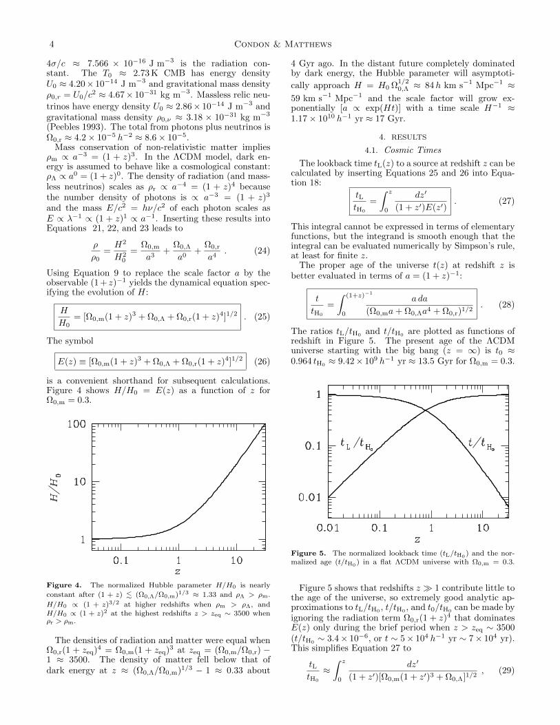
The ratios tL/tH0and t/tH0
are plotted as functions ofredshift in Figure 5. The present age of the ΛCDMuniverse starting with the big bang (z = ∞) is t0 ≈0.964 tH0
≈ 9.42× 10⁹ h−1 yr ≈ 13.5 Gyr for Ω0,m = 0.3.
Figure 5. The normalized lookback time (tL/tH0) and the nor-
malized age (t/tH0 ) in a flat ΛCDM universe with Ω0,m = 0.3.
Figure 5 shows that redshifts z 1 contribute little tothe age of the universe, so extremely good analytic ap-proximations to tL/tH0 , t/tH0 , and t0/tH0 can be made byignoring the radiation term Ω0,r(1 + z)4 that dominatesE(z) only during the brief period when z > zeq ∼ 3500(t/tH0
∼ 3.4× 10⁻⁶, or t ∼ 5× 10⁴ h−1 yr ∼ 7× 10⁴ yr).This simplifies Equation 27 to
tLtH0
≈∫ z
0
dz′
(1 + z′)[Ω0,m(1 + z′)3 + Ω0,Λ]1/2, (29)
ΛCDM Cosmology for Astronomers 5
which can be integrated analytically. See Appendix Afor analytic approximations to tL/tH0 (Equation A5) andt/tH0
(Equation A10). The current age of the universenormalized by the Hubble time is very nearly
t0tH0
≈ 2
3 Ω1/20,Λ
ln
[1 + Ω
1/20,Λ
(1− Ω0,Λ)1/2
]. (30)
Figure 6 plots t0/tH0from Equation 30 as a function of
the matter density parameter Ω0,m = 1 − Ω0,Λ. In thelimit Ω0,m = 1 − Ω0,Λ → 0, the universe would expandexponentially and t0/tH0 would diverge.
Figure 6. The normalized age of the universe t0/tH0as a function
of Ω0,m = 1− Ω0,Λ
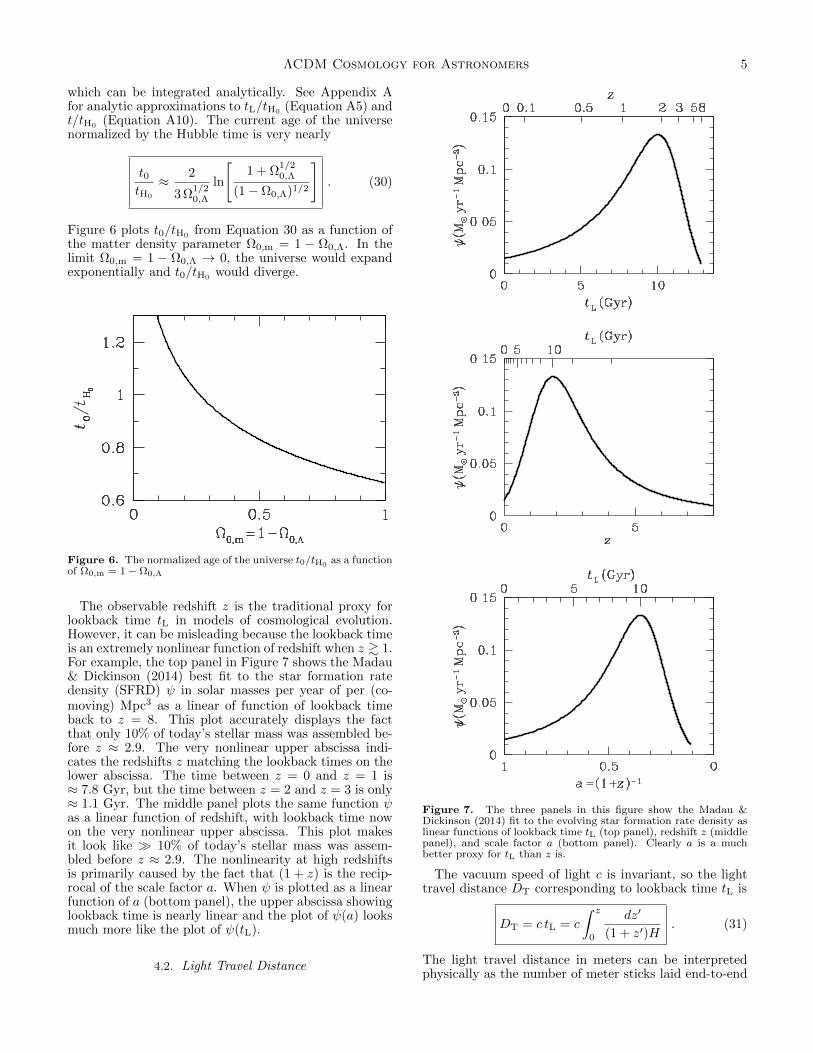
The observable redshift z is the traditional proxy forlookback time tL in models of cosmological evolution.However, it can be misleading because the lookback timeis an extremely nonlinear function of redshift when z & 1.For example, the top panel in Figure 7 shows the Madau& Dickinson (2014) best fit to the star formation ratedensity (SFRD) ψ in solar masses per year of per (co-moving) Mpc3 as a linear of function of lookback timeback to z = 8. This plot accurately displays the factthat only 10% of today’s stellar mass was assembled be-fore z ≈ 2.9. The very nonlinear upper abscissa indi-cates the redshifts z matching the lookback times on thelower abscissa. The time between z = 0 and z = 1 is≈ 7.8 Gyr, but the time between z = 2 and z = 3 is only≈ 1.1 Gyr. The middle panel plots the same function ψas a linear function of redshift, with lookback time nowon the very nonlinear upper abscissa. This plot makesit look like 10% of today’s stellar mass was assem-bled before z ≈ 2.9. The nonlinearity at high redshiftsis primarily caused by the fact that (1 + z) is the recip-rocal of the scale factor a. When ψ is plotted as a linearfunction of a (bottom panel), the upper abscissa showinglookback time is nearly linear and the plot of ψ(a) looksmuch more like the plot of ψ(tL).
4.2. Light Travel Distance
Figure 7. The three panels in this figure show the Madau &Dickinson (2014) fit to the evolving star formation rate density aslinear functions of lookback time tL (top panel), redshift z (middlepanel), and scale factor a (bottom panel). Clearly a is a muchbetter proxy for tL than z is.
The vacuum speed of light c is invariant, so the lighttravel distance DT corresponding to lookback time tL is
DT = c tL = c
∫ z
0
dz′
(1 + z′)H. (31)
The light travel distance in meters can be interpretedphysically as the number of meter sticks laid end-to-end
6 Condon & Matthews
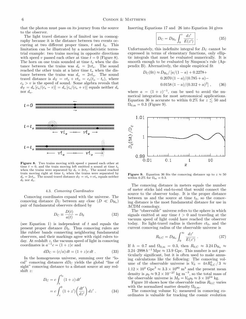
that the photon must pass on its journey from the sourceto the observer.
The light travel distance is of limited use in cosmog-raphy because it is the distance between two events oc-curring at two different proper times, t and t0. Thislimitation can be illustrated by a nonrelativistic terres-trial example: two trains moving in opposite directionswith speed v passed each other at time t = 0 (Figure 8).The horn on one train sounded at time te when the dis-tance between the trains was de = 2vte. The soundreached the other train at a later time to when the dis-tance between the trains was do = 2vto. The soundtravel distance is dT = vte + vto = cs(to − te), wherecs > v is the speed of sound. Some algebra reveals thatdT = de [cs/(cs − v)] = do [cs/(cs + v)] equals neither de
nor do.
Figure 8. Two trains moving with speed v passed each other attime t = 0, and the train moving left emitted a sound at time tewhen the trains were separated by de = 2vte. The sound reachedtrain moving right at time to when the trains were separated bydo = 2vto. The sound travel distance dT = vte +vto equals neitherde nor do.
4.3. Comoving Coordinates
Comoving coordinates expand with the universe. Thecomoving distance DC between any close (D DH0
)pair of fundamental observers defined by
DC ≡D(t)
a(t)= D0 (32)
(see Equation 1) is independent of t and equals thepresent proper distance D0. Thus comoving rulers arelike rubber bands connecting neighboring fundamentalobservers, and their markings agree with rigid rulers to-day. At redshift z, the vacuum speed of light in comovingcoordinates is a−1c = (1 + z)c and
dDC = (c/a) dt = (1 + z)c dt . (33)
In the homogeneous universe, summing over the “lo-cal” comoving distances dDC yields the global “line ofsight” comoving distance to a distant source at any red-shift z:
DC = c
∫ t0
t
(1 + z) dt′
= c
∫ 0
z
(1 + z′)
(dt′
dz′
)dz′ . (34)
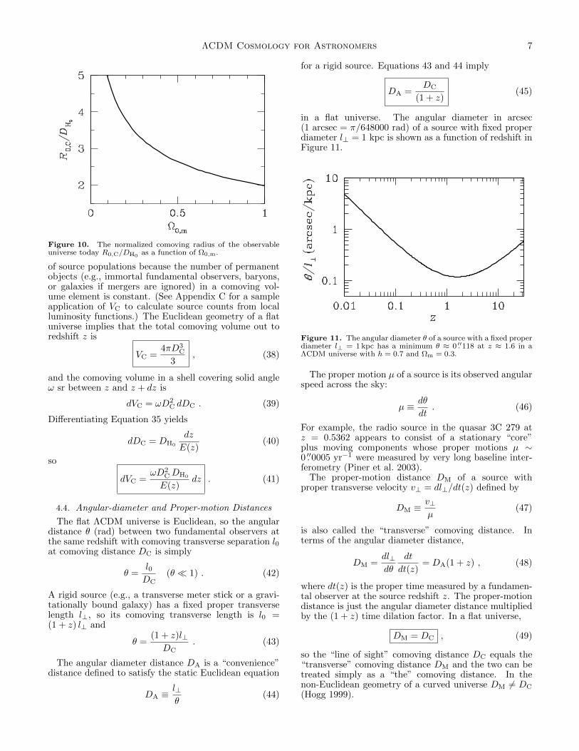
Inserting Equations 17 and 26 into Equation 34 gives
DC = DH0
∫ z
0
dz′
E(z′). (35)
Unfortunately, this indefinite integral for DC cannot beexpressed in terms of elementary functions, only ellip-tic integrals that must be evaluated numerically. It issmooth enough to be evaluated by Simpson’s rule (Ap-pendix B). Alternatively, the simple empirical fit
DC(fit) ≈DH0/ [a/(1− a) + 0.2278+
0.2070 (1− a)/(0.785 + a)−0.0158 (1− a)/(0.312 + a)2] , (36)
where a = (1 + z)−1, can be used to avoid the nu-merical integration for most astronomical applications.Equation 36 is accurate to within 0.2% for z . 50 andΩ0,m = 0.3 (Figure 9).
Figure 9. Equation 36 fits the comoving distance up to z ≈ 50within 0.2% for Ωm = 0.3.
The comoving distance in meters equals the numberof meter sticks laid end-to-end that would connect thesource to the observer today. It is the proper distancebetween us and the source at time t0, so the comov-ing distance is the most fundamental distance for use inΛCDM cosmology.
The “observable” universe refers to the sphere in whichsignals emitted at any time t > 0 and traveling at thevacuum speed of light could have reached the observertoday. Its light-travel radius is therefore ct0, and thecurrent comoving radius of the observable universe is
R0,C = DH0
∫ ∞0
dz′
E(z′). (37)
If h = 0.7 and Ω0,m = 0.3, then R0,C ≈ 3.24DH0≈
3.24 ·2998h−1 Mpc ≈ 13.9 Gpc. This number is not par-ticularly significant, but it is often used to make amus-ing calculations like the following: The comoving vol-ume of the observable universe is V0 = 4πR3
0,C / 3 ≈1.12 × 10⁴ Gpc3 ≈ 3.3 × 1080 m3 and the present meandensity is ρ0 ≈ 9.2× 10⁻²⁷ kg m−3, so the total mass ofthe observable universe is M0 = V0ρ0 ≈ 3× 1054 kg.
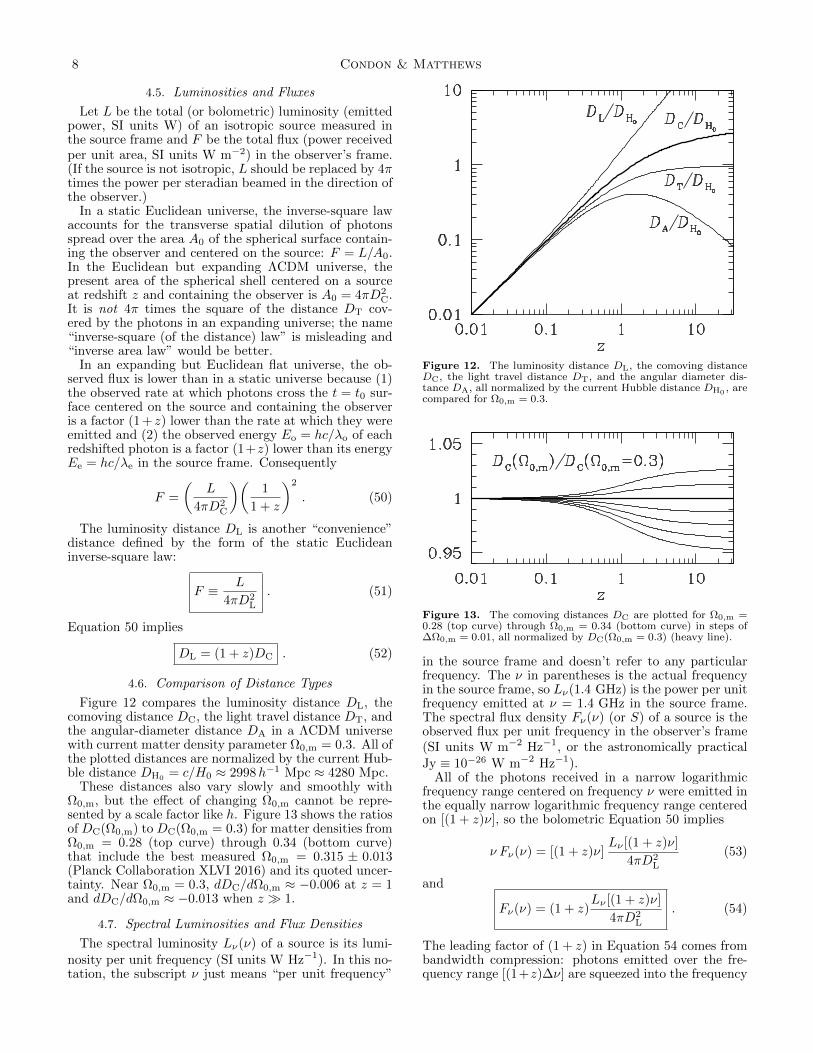
Figure 10 shows how the observable radius R0,C varieswith the normalized matter density Ω0,m.
The comoving volume VC measured in comoving co-ordinates is valuable for tracking the cosmic evolution
ΛCDM Cosmology for Astronomers 7
Figure 10. The normalized comoving radius of the observableuniverse today R0,C/DH0 as a function of Ω0,m.
of source populations because the number of permanentobjects (e.g., immortal fundamental observers, baryons,or galaxies if mergers are ignored) in a comoving vol-ume element is constant. (See Appendix C for a sampleapplication of VC to calculate source counts from localluminosity functions.) The Euclidean geometry of a flatuniverse implies that the total comoving volume out toredshift z is
VC =4πD3
C
3, (38)
and the comoving volume in a shell covering solid angleω sr between z and z + dz is
dVC = ωD2C dDC . (39)
Differentiating Equation 35 yields
dDC = DH0
dz
E(z)(40)
so
dVC =ωD2
CDH0
E(z)dz . (41)
4.4. Angular-diameter and Proper-motion Distances
The flat ΛCDM universe is Euclidean, so the angulardistance θ (rad) between two fundamental observers atthe same redshift with comoving transverse separation l0at comoving distance DC is simply
θ =l0DC
(θ 1) . (42)
A rigid source (e.g., a transverse meter stick or a gravi-tationally bound galaxy) has a fixed proper transverselength l⊥, so its comoving transverse length is l0 =(1 + z) l⊥ and
θ =(1 + z)l⊥DC
. (43)
The angular diameter distance DA is a “convenience”distance defined to satisfy the static Euclidean equation
DA ≡l⊥θ
(44)
for a rigid source. Equations 43 and 44 imply
DA =DC
(1 + z)(45)
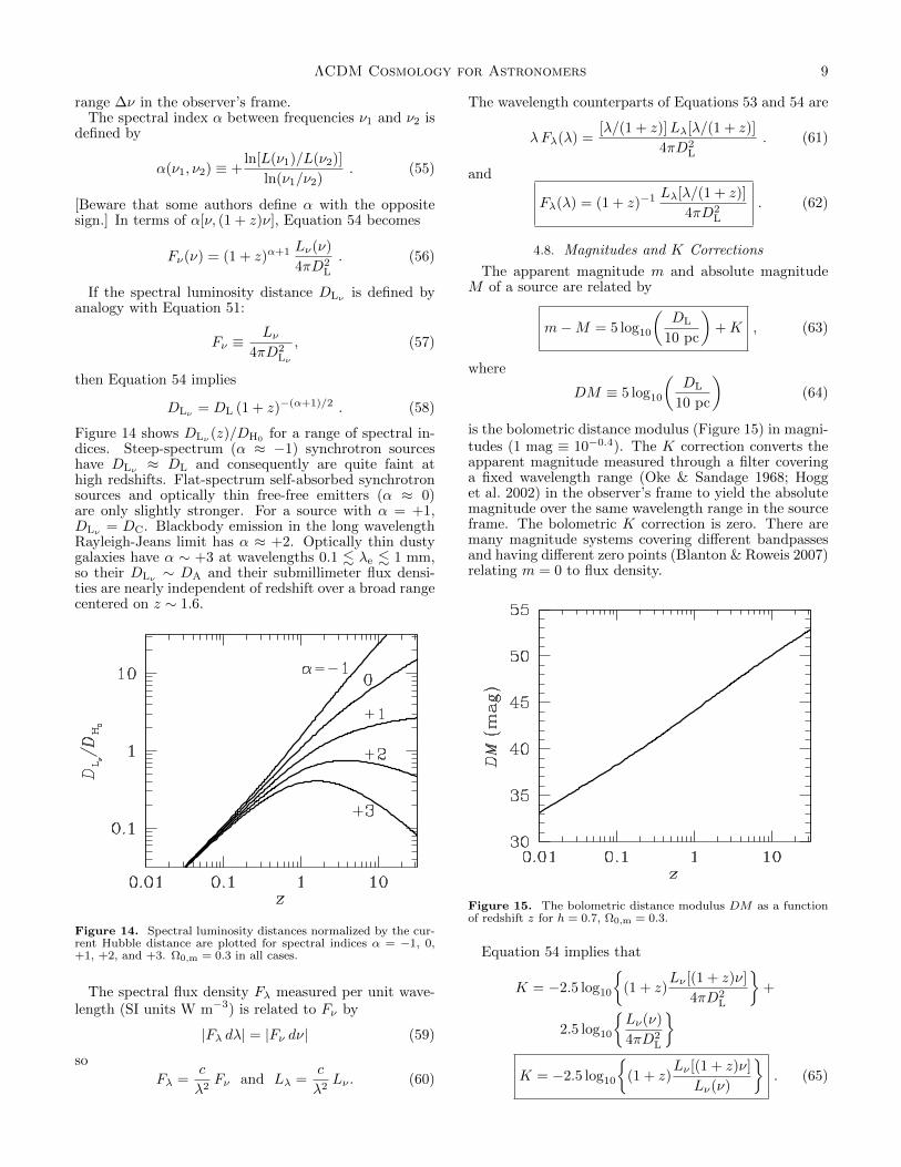
in a flat universe. The angular diameter in arcsec(1 arcsec = π/648000 rad) of a source with fixed properdiameter l⊥ = 1 kpc is shown as a function of redshift inFigure 11.
Figure 11. The angular diameter θ of a source with a fixed properdiameter l⊥ = 1 kpc has a minimum θ ≈ 0 .′′118 at z ≈ 1.6 in aΛCDM universe with h = 0.7 and Ωm = 0.3.
The proper motion µ of a source is its observed angularspeed across the sky:
µ ≡ dθ
dt. (46)
For example, the radio source in the quasar 3C 279 atz = 0.5362 appears to consist of a stationary “core”plus moving components whose proper motions µ ∼0 .′′0005 yr−1 were measured by very long baseline inter-ferometry (Piner et al. 2003).
The proper-motion distance DM of a source withproper transverse velocity v⊥ = dl⊥/dt(z) defined by
DM ≡v⊥µ
(47)
is also called the “transverse” comoving distance. Interms of the angular diameter distance,
DM =dl⊥dθ
dt
dt(z)= DA(1 + z) , (48)
where dt(z) is the proper time measured by a fundamen-tal observer at the source redshift z. The proper-motiondistance is just the angular diameter distance multipliedby the (1 + z) time dilation factor. In a flat universe,
DM = DC , (49)
so the “line of sight” comoving distance DC equals the“transverse” comoving distance DM and the two can betreated simply as a “the” comoving distance. In thenon-Euclidean geometry of a curved universe DM 6= DC
(Hogg 1999).
8 Condon & Matthews
4.5. Luminosities and Fluxes
Let L be the total (or bolometric) luminosity (emittedpower, SI units W) of an isotropic source measured inthe source frame and F be the total flux (power receivedper unit area, SI units W m−2) in the observer’s frame.(If the source is not isotropic, L should be replaced by 4πtimes the power per steradian beamed in the direction ofthe observer.)
In a static Euclidean universe, the inverse-square lawaccounts for the transverse spatial dilution of photonsspread over the area A0 of the spherical surface contain-ing the observer and centered on the source: F = L/A0.In the Euclidean but expanding ΛCDM universe, thepresent area of the spherical shell centered on a sourceat redshift z and containing the observer is A0 = 4πD2
C.It is not 4π times the square of the distance DT cov-ered by the photons in an expanding universe; the name“inverse-square (of the distance) law” is misleading and“inverse area law” would be better.
In an expanding but Euclidean flat universe, the ob-served flux is lower than in a static universe because (1)the observed rate at which photons cross the t = t0 sur-face centered on the source and containing the observeris a factor (1 + z) lower than the rate at which they wereemitted and (2) the observed energy Eo = hc/λo of eachredshifted photon is a factor (1+z) lower than its energyEe = hc/λe in the source frame. Consequently
F =
(L
4πD2C
)(1
1 + z
)2
. (50)
The luminosity distance DL is another “convenience”distance defined by the form of the static Euclideaninverse-square law:
F ≡ L
4πD2L
. (51)
Equation 50 implies
DL = (1 + z)DC . (52)
4.6. Comparison of Distance Types
Figure 12 compares the luminosity distance DL, thecomoving distance DC, the light travel distance DT, andthe angular-diameter distance DA in a ΛCDM universewith current matter density parameter Ω0,m = 0.3. All ofthe plotted distances are normalized by the current Hub-ble distance DH0 = c/H0 ≈ 2998h−1 Mpc ≈ 4280 Mpc.
These distances also vary slowly and smoothly withΩ0,m, but the effect of changing Ω0,m cannot be repre-sented by a scale factor like h. Figure 13 shows the ratiosof DC(Ω0,m) to DC(Ω0,m = 0.3) for matter densities fromΩ0,m = 0.28 (top curve) through 0.34 (bottom curve)that include the best measured Ω0,m = 0.315 ± 0.013(Planck Collaboration XLVI 2016) and its quoted uncer-tainty. Near Ω0,m = 0.3, dDC/dΩ0,m ≈ −0.006 at z = 1and dDC/dΩ0,m ≈ −0.013 when z 1.
4.7. Spectral Luminosities and Flux Densities
The spectral luminosity Lν(ν) of a source is its lumi-nosity per unit frequency (SI units W Hz−1). In this no-tation, the subscript ν just means “per unit frequency”
Figure 12. The luminosity distance DL, the comoving distanceDC, the light travel distance DT, and the angular diameter dis-tance DA, all normalized by the current Hubble distance DH0
, arecompared for Ω0,m = 0.3.
Figure 13. The comoving distances DC are plotted for Ω0,m =0.28 (top curve) through Ω0,m = 0.34 (bottom curve) in steps of∆Ω0,m = 0.01, all normalized by DC(Ω0,m = 0.3) (heavy line).
in the source frame and doesn’t refer to any particularfrequency. The ν in parentheses is the actual frequencyin the source frame, so Lν(1.4 GHz) is the power per unitfrequency emitted at ν = 1.4 GHz in the source frame.The spectral flux density Fν(ν) (or S) of a source is theobserved flux per unit frequency in the observer’s frame(SI units W m−2 Hz−1, or the astronomically practicalJy ≡ 10−26 W m−2 Hz−1).
All of the photons received in a narrow logarithmicfrequency range centered on frequency ν were emitted inthe equally narrow logarithmic frequency range centeredon [(1 + z)ν], so the bolometric Equation 50 implies
ν Fν(ν) = [(1 + z)ν]Lν [(1 + z)ν]
4πD2L
(53)
and
Fν(ν) = (1 + z)Lν [(1 + z)ν]
4πD2L
. (54)
The leading factor of (1 + z) in Equation 54 comes frombandwidth compression: photons emitted over the fre-quency range [(1+z)∆ν] are squeezed into the frequency
ΛCDM Cosmology for Astronomers 9
range ∆ν in the observer’s frame.The spectral index α between frequencies ν1 and ν2 is
defined by
α(ν1, ν2) ≡ +ln[L(ν1)/L(ν2)]
ln(ν1/ν2). (55)
[Beware that some authors define α with the oppositesign.] In terms of α[ν, (1 + z)ν], Equation 54 becomes
Fν(ν) = (1 + z)α+1 Lν(ν)
4πD2L
. (56)
If the spectral luminosity distance DLν is defined byanalogy with Equation 51:
Fν ≡Lν
4πD2Lν
, (57)
then Equation 54 implies
DLν = DL (1 + z)−(α+1)/2 . (58)
Figure 14 shows DLν (z)/DH0 for a range of spectral in-dices. Steep-spectrum (α ≈ −1) synchrotron sourceshave DLν ≈ DL and consequently are quite faint athigh redshifts. Flat-spectrum self-absorbed synchrotronsources and optically thin free-free emitters (α ≈ 0)are only slightly stronger. For a source with α = +1,DLν = DC. Blackbody emission in the long wavelengthRayleigh-Jeans limit has α ≈ +2. Optically thin dustygalaxies have α ∼ +3 at wavelengths 0.1 . λe . 1 mm,so their DLν ∼ DA and their submillimeter flux densi-ties are nearly independent of redshift over a broad rangecentered on z ∼ 1.6.
Figure 14. Spectral luminosity distances normalized by the cur-rent Hubble distance are plotted for spectral indices α = −1, 0,+1, +2, and +3. Ω0,m = 0.3 in all cases.
The spectral flux density Fλ measured per unit wave-length (SI units W m−3) is related to Fν by
|Fλ dλ| = |Fν dν| (59)
so
Fλ =c
λ2Fν and Lλ =
c
λ2Lν . (60)
The wavelength counterparts of Equations 53 and 54 are
λFλ(λ) =[λ/(1 + z)]Lλ[λ/(1 + z)]
4πD2L
. (61)
and
Fλ(λ) = (1 + z)−1 Lλ[λ/(1 + z)]
4πD2L
. (62)
4.8. Magnitudes and K Corrections
The apparent magnitude m and absolute magnitudeM of a source are related by
m−M = 5 log10
(DL
10 pc
)+K , (63)
where
DM ≡ 5 log10
(DL
10 pc
)(64)
is the bolometric distance modulus (Figure 15) in magni-tudes (1 mag ≡ 10−0.4). The K correction converts theapparent magnitude measured through a filter coveringa fixed wavelength range (Oke & Sandage 1968; Hogget al. 2002) in the observer’s frame to yield the absolutemagnitude over the same wavelength range in the sourceframe. The bolometric K correction is zero. There aremany magnitude systems covering different bandpassesand having different zero points (Blanton & Roweis 2007)relating m = 0 to flux density.
Figure 15. The bolometric distance modulus DM as a functionof redshift z for h = 0.7, Ω0,m = 0.3.
Equation 54 implies that
K = −2.5 log10
(1 + z)
Lν [(1 + z)ν]
4πD2L
+
2.5 log10
Lν(ν)
4πD2L
K = −2.5 log10
(1 + z)
Lν [(1 + z)ν]
Lν(ν)
. (65)
10 Condon & Matthews
In terms of the spectral index α,
K = −2.5 log10
[(1 + z)α+1
]= −2.5 (α+ 1) log10(1 + z) . (66)
In terms of wavelengths,
K = −2.5 log10
(1 + z)−1Lλ[λ/(1 + z)]
Lλ(λ)
. (67)
4.9. Spectral Lines
Spectral lines are narrow (line width ∆ν ν) emissionor absorption features in the spectra of gaseous or ionizedsources. The total line luminosity L is related to the totalline flux F and the line flux density Fν by Equation 51,so
L = 4πD2LF = 4πD2
L Fν∆ν . (68)
In Equation 68, the SI units of F are W m−2 =1026 Jy Hz. However, line fluxes are often reported inthe dimensionally confusing units Jy km s−1 based onthe nonrelativistic Doppler equation
∆ν
ν≈ ∆v
c 1 . (69)
Solving Equation 69 for ∆v yields the factor needed toconvert from Jy km s−1 to Jy Hz:
1 km s−1 ≈ ν
299792Hz . (70)
See Carilli & Walter (2013) for a detailed discussion ofthis equation and its uses.
4.10. Total Intensity and Specific Intensity
The total intensity or bolometric brightness B of asource is the power it emits per unit area per unit solidangle ω (SI units W m−2 sr−1). In a static Euclidianuniverse, intensity is conserved along any ray passingthrough empty space and the brightness B0 seen by anobserver at rest with respect to the source equals B. Fora source at redshift z in the Euclidean but expandingΛCDM universe, the observed brightness B0 can be cal-culated with the aid of Equations 45 and 52. For a sourceat any comoving distance DC, expansion multiplies itsluminosity distance by (1 + z) and divides its angulardiameter distance by (1 + z), so
B0
B=F0
F
ω
ω0= (1 + z)−2(1 + z)−2 (71)
andB0
B= (1 + z)−4 . (72)
The specific intensity or spectral brightness Bν(ν) ofa source is its power per unit frequency per unit solidangle (SI units W m−2 Hz−1 sr−1) at frequency ν in thesource frame.
All of the photons received in a narrow logarithmicfrequency range centered on ν were emitted in the equallynarrow logarithmic frequency range centered on [(1 +z)ν], so the bolometric brightness Equation 72 implies
νBν0 =[(1 + z)ν]Bν [(1 + z)ν]
(1 + z)4. (73)
Bν0(ν) = (1 + z)−3Bν [(1 + z)ν] . (74)
For a source with spectral index α,
Bν0(ν) = (1 + z)α−3Bν(ν) . (75)
The Planck brightness spectrum of a blackbody sourceat temperature T is
Bν(ν |T ) =2hν3
c2
[exp
(hν
kT
)− 1
]−1
. (76)
If the source is at redshift z, the observed spectrum
Bν0(ν) = (1 + z)−3Bν [(1 + z)ν |T ]
=2h
c2
[(1 + z)ν
(1 + z)
]3exp
[hν
k
(1 + z)
T
]− 1
−1
(77)
is just the Planck spectrum Bν(ν|T0) of a blackbodywith temperature T0 = T/(1 + z). The source of theT0 ≈ 2.73 K CMB seen today is the T ∼ 3000 K black-body surface of last scattering when the universe becametransparent at z ∼ 1100.
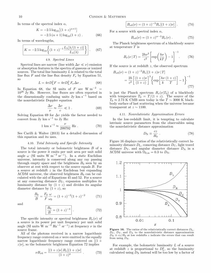
4.11. Nonrelativistic Approximation Errors
In the low-redshift limit, it is tempting to calculateintrinsic source parameters from the observables usingthe nonrelativistic distance approximation
DN ≡cz
H0. (78)
Figure 16 displays ratios of the relativistically correct lu-minosity distance DL, comoving distance DC, light traveldistance DT, and angular diameter distance DA in aΛCDM universe with Ω0,m = 0.3 to DN.
Figure 16. The ratios of the relativistically correct distances DL,DC, DT, and DA to the nonrelativistic distance approximationDN ≡ cz/H0 at low redshifts z indicate the errors that can resultfrom using DN.
For example, the bolometric luminosity L of a sourceat redshift z is proportional to D2
L, so the luminositycalculated using DN instead will be too low by a factor of
ΛCDM Cosmology for Astronomers 11
(DL/DN)2. It will be 5% too low for a source at redshiftz ≈ 0.032 (cz ∼ 104 km s−1), and the maximum redshiftat which the luminosity error is < 10% is z ≈ 0.065(cz ∼ 2× 10⁴ km s−1).
The calculated linear size of a source is proportionalto DA < DN, so using DN will overestimate source sizeby 5% at z ≈ 0.043 (cz ∼ 1.3× 10⁴ km s−1) and 10% atz ≈ 0.089 (cz ∼ 2.7× 10⁴ km s−1).
Such errors are systematic, so they can easily dominatethe Poisson errors in statistical properties of large sourcepopulations. Luminosity functions are particularly vul-nerable because they depend on the maximum redshiftsat which sources could have remained in the flux-limitedpopulation, not just the actual source redshifts.
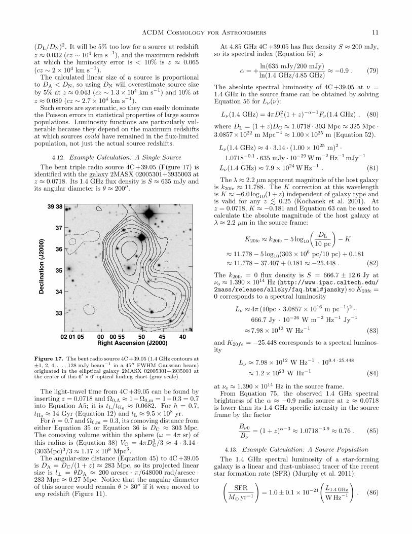
4.12. Example Calculation: A Single Source
The bent triple radio source 4C +39.05 (Figure 17) isidentified with the galaxy 2MASX 02005301+3935003 atz ≈ 0.0718. Its 1.4 GHz flux density is S ≈ 635 mJy andits angular diameter is θ ≈ 200′′.
Dec
linat
ion
(J20
00)
Right Ascension (J2000)02 01 05 00 00 55 50 45 40
39 38
37
36
35
34
33
Figure 17. The bent radio source 4C +39.05 (1.4 GHz contours at±1, 2, 4, . . . , 128 mJy beam−1 in a 45′′ FWHM Gaussian beam)originated in the elliptical galaxy 2MASX 02005301+3935003 atthe center of this 6′ × 6′ optical finding chart (gray scale).
The light-travel time from 4C +39.05 can be found byinserting z = 0.0718 and Ω0,Λ ≈ 1−Ω0,m = 1−0.3 = 0.7into Equation A5; it is tL/tH0
≈ 0.0682. For h = 0.7,tH0 ≈ 14 Gyr (Equation 12) and tL ≈ 9.5× 10⁸ yr.
For h = 0.7 and Ω0,m = 0.3, its comoving distance fromeither Equation 35 or Equation 36 is DC ≈ 303 Mpc.The comoving volume within the sphere (ω = 4π sr) ofthis radius is (Equation 38) VC = 4πD3
C/3 ≈ 4 · 3.14 ·(303Mpc)3/3 ≈ 1.17× 10⁸ Mpc3.
The angular-size distance (Equation 45) to 4C +39.05is DA = DC/(1 + z) ≈ 283 Mpc, so its projected linearsize is l⊥ = θDA ≈ 200 arcsec · π/648000 rad/arcsec ·283 Mpc ≈ 0.27 Mpc. Notice that the angular diameterof this source would remain θ > 30′′ if it were moved toany redshift (Figure 11).
At 4.85 GHz 4C +39.05 has flux density S ≈ 200 mJy,so its spectral index (Equation 55) is
α = +ln(635 mJy/200 mJy)
ln(1.4 GHz/4.85 GHz)≈ −0.9 . (79)
The absolute spectral luminosity of 4C +39.05 at ν =1.4 GHz in the source frame can be obtained by solvingEquation 56 for Lν(ν):
Lν(1.4 GHz) = 4πD2L(1 + z)−α−1Fν(1.4 GHz) , (80)
where DL = (1 + z)DC ≈ 1.0718 · 303 Mpc ≈ 325 Mpc ·3.0857× 1022 m Mpc−1 ≈ 1.00× 1025 m (Equation 52).
Lν(1.4 GHz) ≈ 4 · 3.14 · (1.00× 1025 m)2 ·1.0718−0.1 · 635 mJy · 10−29 W m−2 Hz−1 mJy−1
Lν(1.4 GHz) ≈ 7.9× 1024 W Hz−1 . (81)
The λ ≈ 2.2 µm apparent magnitude of the host galaxyis k20fe ≈ 11.788. The K correction at this wavelengthis K ≈ −6.0 log10(1 + z) independent of galaxy type andis valid for any z . 0.25 (Kochanek et al. 2001). Atz = 0.0718, K ≈ −0.181 and Equation 63 can be used tocalculate the absolute magnitude of the host galaxy atλ ≈ 2.2 µm in the source frame:
K20fe ≈ k20fe − 5 log10
(DL
10 pc
)−K
≈ 11.778− 5 log10(303× 106 pc/10 pc) + 0.181
≈ 11.778− 37.407 + 0.181 ≈ −25.448 . (82)
The k20fe = 0 flux density is S = 666.7 ± 12.6 Jy atνo ≈ 1.390× 10¹⁴ Hz (http://www.ipac.caltech.edu/2mass/releases/allsky/faq.html#jansky) soK20fe =0 corresponds to a spectral luminosity
Lν ≈ 4π (10pc · 3.0857× 1016 m pc−1)2 ·666.7 Jy · 10−26 W m−2 Hz−1 Jy−1
≈ 7.98× 10¹² W Hz−1 (83)
and K20fe = −25.448 corresponds to a spectral luminos-ity
Lν ≈ 7.98× 10¹² W Hz−1 · 100.4 · 25.448
≈ 1.2× 10²³ W Hz−1 (84)
at νe ≈ 1.390× 10¹⁴ Hz in the source frame.From Equation 75, the observed 1.4 GHz spectral
brightness of the α ≈ −0.9 radio source at z ≈ 0.0718is lower than its 1.4 GHz specific intensity in the sourceframe by the factor
Bν0
Bν= (1 + z)α−3 ≈ 1.0718−3.9 ≈ 0.76 . (85)
4.13. Example Calculation: A Source Population
The 1.4 GHz spectral luminosity of a star-forminggalaxy is a linear and dust-unbiased tracer of the recentstar formation rate (SFR) (Murphy et al. 2011):(
SFR
M yr−1
)= 1.0± 0.1× 10⁻²¹
(L1.4 GHz
W Hz−1
). (86)
12 Condon & Matthews
If the comoving space density of 1.4 GHz sources in star-forming galaxies is ρ(L1.4 GHz), then the local luminosity-weighted spectral power density function (Equation C8)is
Udex(Lν | z) = ln(10)L2νρ(Lν | z) . (87)
Figure 18. The local 1.4 GHz spectral energy density functionUdex of galaxies whose radio emission is powered primarily by starformation, not by AGNs.
The observed Udex(L1.4 GHz | z ≈ 0) (Condon &Matthews 2018) is shown by the data points in Figure 18,and it can be approximated by the function (dotted curvein Figure 18)
Udex(L1.4 GHz | z ≈ 0) ≈ L1.4 GHz(W Hz−1) ·
4.0× 10−3 Mpc−3 dex−1
(L1.4 GHz
L∗ν
)β·
exp
[− 1
2σ2log2
(1 +
L1.4 GHz
L∗ν
)], (88)
where L∗1.4 GHz = 1.7 × 10²¹ W Hz−1, β = −0.24, andσ = 0.585.
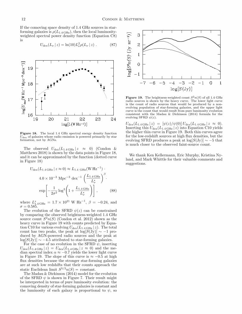
The evolution of the SFRD ψ(z) can be constrainedby comparing the observed brightness-weighted 1.4 GHzsource count S2n(S) (Condon et al. 2012) shown as theheavy curve in Figure 19 with counts predicted by Equa-tion C10 for various evolving Udex(L1.4 GHz | z). The totalcount has two peaks, the peak at log[S(Jy)] ∼ −1 pro-duced by AGN-powered radio sources and the peak atlog[S(Jy)] ∼ −4.5 attributed to star-forming galaxies.
For the case of no evolution in the SFRD ψ, insertingUdex(L1.4 GHz | z) = Udex(L1.4 GHz | z ≈ 0) and the me-dian spectral index α ≈ −0.7 yields the lower light curvein Figure 19. The slope of this curve is ≈ −0.5 at highflux densities because the stronger star-forming galaxiesare at such low redshifts that their counts approach thestatic Euclidean limit S5/2n(S) = constant.
The Madau & Dickinson (2014) model for the evolutionof the SFRD ψ is shown in Figure 7. Their result mightbe interpreted in terms of pure luminosity evolution: thecomoving density of star-forming galaxies is constant andthe luminosity of each galaxy is proportional to ψ, so
Figure 19. The brightness-weighted count S2n(S) of all 1.4 GHzradio sources is shown by the heavy curve. The lower light curveis the count of radio sources that would be produced by a non-evolving population of star-forming galaxies, and the upper lightcurve is the count that would result from pure luminosity evolutionconsistent with the Madau & Dickinson (2014) formula for theevolving SFRD ψ(z).
Udex(L1.4 GHz | z) = [ψ(z)/ψ(0)]Udex(L1.4 GHz | z ≈ 0).Inserting this Udex(L1.4 GHz | z) into Equation C10 yieldsthe higher thin curve in Figure 19. Both thin curves agreefor the low-redshift sources at high flux densities, but theevolving SFRD produces a peak at log[S(Jy)] ∼ −5 thatis much closer to the observed faint-source count.
We thank Ken Kellermann, Eric Murphy, Kristina Ny-land, and Mark Whittle for their valuable comments andsuggestions.
ΛCDM Cosmology for Astronomers 13
APPENDIX
ANALYTIC APPROXIMATIONS FOR LOOKBACK TIME AND AGE
Equation 18 for the lookback time tL:
tL =DL
c= tH0
∫ z
0
dz′
(1 + z′)E(z′)(A1)
can be integrated analytically if the currently small radiation term Ω0,r is ignored in E(z′). Then
tLtH0
≈∫ z
0
dz′
(1 + z′)[Ω0,m(1 + z′)3 + Ω0,Λ]1/2. (A2)
Substituting Ω0,Λ = 1− Ω0,m and x = (1 + z′)−3/2 reduces Equation A2 to
tLtH0
≈ 2
3 Ω1/20,Λ
∫ 1
(1+z)−3/2
dx√(1− Ω0,Λ)/Ω0,Λ + x2
. (A3)
The indefinite integral ∫dx√a2 + x2
= ln(x+
√a2 + x2
)+ C . (A4)
can be found in integral tables or evaluated via the trigonometric substitution x = a tan(u). Thus
tLtH0
≈ 2
3 Ω1/20,Λ
ln
[1 + Ω
−1/20,Λ
(1 + z)−3/2 +√
(1 + z)−3 + (1− Ω0,Λ)/Ω0,Λ
](A5)
In the limit z →∞, tL becomes the present age of the universe t0:
t0tH0
≈ 2
3 Ω1/20,Λ
ln
[1 + Ω
1/20,Λ
(1− Ω0,Λ)1/2
]. (A6)
The fractional errors in Equations A5 and A6 are < 10−3 for all z and all Ω0,m > 0.1 only because the high redshifts atwhich the omitted Ω0,r(1 + z′)4 term is significant contribute little to tL and t0. Equation A5 can be used to calculateaccurate lookback time differences ∆tL = tL(z + ∆z) − tL(z) only if z 3500. The fractional errors in differentiallookback times are < 10−3 if z < 10 and rise to 10−2 at z ∼ 60 and to 10−1 at z ∼ 500.
The age of the universe at redshift z was
t
tH0
≈∫ ∞z
dz′
(1 + z′)[Ω0,m(1 + z′)3 + Ω0,Λ]1/2(A7)
without the radiation term Ω0,r(1 + z′)4. This approximation is safe at redshifts z . 25 (t & 0.045 tH0 ∼ 6 × 10⁸ yr)because radiation dominated E(z) for only the first t ∼ 3.4× 10⁻⁶ tH ∼ 5× 10⁴ h−1 yr ∼ 7× 10⁴ yr after the big bang(Section 4.1).
t
tH0
≈∫ (1+z)−1
0
a1/2 da
[(1− Ω0,Λ) + Ω0,Λa3]1/2. (A8)
Substituting x ≡ a3/2Ω1/20,Λ yields the elementary form
t
tH0
≈ 2
3 Ω1/20,Λ
∫ (1+z)−3/2Ω1/2Λ
0
dx
[(1− Ω0,Λ) + x2]1/2. (A9)
This is similar to Equation A4, so
t
tH0
≈ 2
3 Ω1/2Λ
ln
(Ω0,Λ
1− Ω0,Λ
)1/2
(1 + z)−3/2 +
[Ω0,Λ
(1 + z)3 (1− Ω0,Λ)+ 1
]1/2
. (A10)
Equation A10 directly gives the same t0/tH0as Equation A6, t/tH0
with fractional errors < 10−2 for all z < 25, andsmaller errors in time differences ∆t = −∆tL at high z than Equation A5.
14 Condon & Matthews
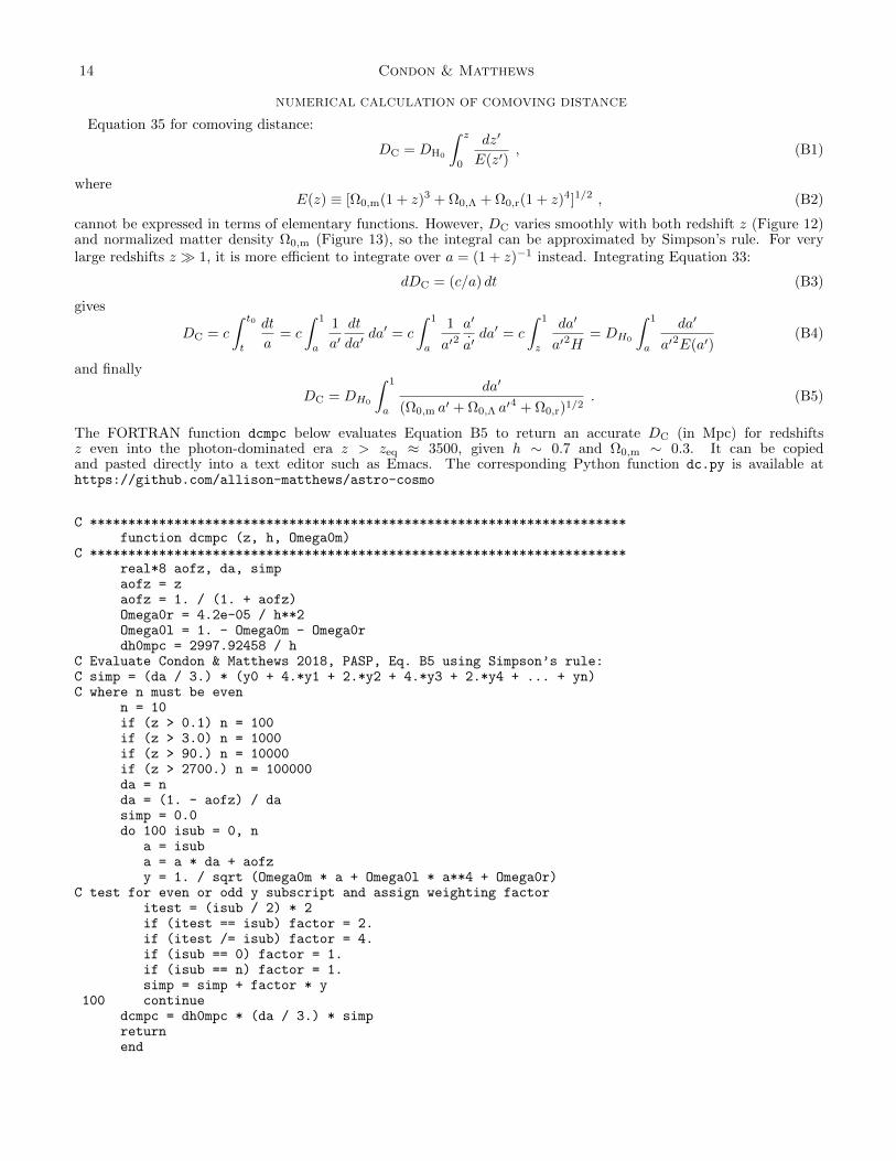
NUMERICAL CALCULATION OF COMOVING DISTANCE
Equation 35 for comoving distance:
DC = DH0
∫ z
0
dz′
E(z′), (B1)
whereE(z) ≡ [Ω0,m(1 + z)3 + Ω0,Λ + Ω0,r(1 + z)4]1/2 , (B2)
cannot be expressed in terms of elementary functions. However, DC varies smoothly with both redshift z (Figure 12)and normalized matter density Ω0,m (Figure 13), so the integral can be approximated by Simpson’s rule. For verylarge redshifts z 1, it is more efficient to integrate over a = (1 + z)−1 instead. Integrating Equation 33:
dDC = (c/a) dt (B3)
gives
DC = c
∫ t0
t
dt
a= c
∫ 1
a
1
a′dt
da′da′ = c
∫ 1
a
1
a′2a′
a′da′ = c
∫ 1
z
da′
a′2H= DH0
∫ 1
a
da′
a′2E(a′)(B4)
and finally
DC = DH0
∫ 1
a
da′
(Ω0,m a′ + Ω0,Λ a′4 + Ω0,r)1/2
. (B5)
The FORTRAN function dcmpc below evaluates Equation B5 to return an accurate DC (in Mpc) for redshiftsz even into the photon-dominated era z > zeq ≈ 3500, given h ∼ 0.7 and Ω0,m ∼ 0.3. It can be copiedand pasted directly into a text editor such as Emacs. The corresponding Python function dc.py is available athttps://github.com/allison-matthews/astro-cosmo
C **********************************************************************function dcmpc (z, h, Omega0m)
C **********************************************************************real*8 aofz, da, simpaofz = zaofz = 1. / (1. + aofz)Omega0r = 4.2e-05 / h**2Omega0l = 1. - Omega0m - Omega0rdh0mpc = 2997.92458 / h
C Evaluate Condon & Matthews 2018, PASP, Eq. B5 using Simpson’s rule:C simp = (da / 3.) * (y0 + 4.*y1 + 2.*y2 + 4.*y3 + 2.*y4 + ... + yn)C where n must be even
n = 10if (z > 0.1) n = 100if (z > 3.0) n = 1000if (z > 90.) n = 10000if (z > 2700.) n = 100000da = nda = (1. - aofz) / dasimp = 0.0do 100 isub = 0, n
a = isuba = a * da + aofzy = 1. / sqrt (Omega0m * a + Omega0l * a**4 + Omega0r)
C test for even or odd y subscript and assign weighting factoritest = (isub / 2) * 2if (itest == isub) factor = 2.if (itest /= isub) factor = 4.if (isub == 0) factor = 1.if (isub == n) factor = 1.simp = simp + factor * y
100 continuedcmpc = dh0mpc * (da / 3.) * simpreturnend
ΛCDM Cosmology for Astronomers 15
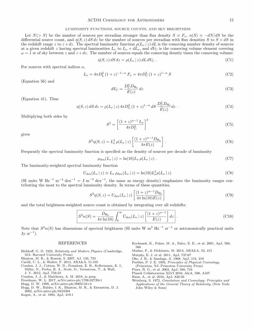
LUMINOSITY FUNCTIONS, SOURCE COUNTS, AND SKY BRIGHTNESS
Let N(> S) be the number of sources per steradian stronger than flux density S ≡ Fν , n(S) ≡ −dN/dS be thedifferential source count, and η(S, z) dS dz be the number of sources per steradian with flux densities S to S + dS inthe redshift range z to z+dz. The spectral luminosity function ρ(Lν | z) dL is the comoving number density of sourcesat a given redshift z having spectral luminosities Lν to Lν + dLν , and dVC is the comoving volume element coveringω = 1 sr of sky between z and z+dz. The number of sources equals the comoving density times the comoving volume:
η(S, z) dS dz = ρ(Lν | z) dLdVC . (C1)
For sources with spectral indices α,
Lν = 4πD2L (1 + z)−1−α Fν = 4πD2
C (1 + z)1−α S (C2)
(Equation 56) and
dVC =D2
CDH0
E(z)dz (C3)
(Equation 41). Thus
η(S, z) dS dz = ρ(Lν | z) 4πD2C (1 + z)1−α dS
D2CDH0
E(z)dz . (C4)
Multiplying both sides by
S2 =
[(1 + z)α−1 Lν
4πD2C
]2
(C5)
gives
S2η(S, z) = L2ν ρ(Lν | z)
[(1 + z)α−1DH0
4πE(z)
]. (C6)
Frequently the spectral luminosity function is specified as the density of sources per decade of luminosity
ρdex(Lν | z) = ln(10)Lν ρ(Lν | z) . (C7)
The luminosity-weighted spectral luminosity function
Udex(Lν | z) ≡ Lν ρdex(Lν | z) = ln(10)L2νρ(Lν | z) (C8)
(SI units W Hz−1 m−3 dex−1 = J m−3 dex−1, the same as energy density) emphasizes the luminosity ranges con-tributing the most to the spectral luminosity density. In terms of these quantities,
S2η(S, z) = Udex(Lν | z)[
(1 + z)α−1DH0
4π ln(10)E(z)
](C9)
and the total brightness-weighted source count is obtained by integrating over all redshifts:
S2n(S) =DH0
4π ln(10)
∫ ∞0
Udex(Lν | z)[
(1 + z)α−1
E(z)
]dz . (C10)
Note that S2n(S) has dimensions of spectral brightness (SI units W m2 Hz−1 sr−1 or astronomically practical unitsJy sr−1).
REFERENCES
Birkhoff, G. D. 1923, Relativity and Modern Physics (Cambridge,MA: Harvard University Press)
Blanton, M. R., & Roweis, S. 2007, AJ, 133, 734Carilli, C. L., & Walter, F. 2013, ARA&A, 51:105Condon, J. J., Cotton, W. D., Fomalont, E. B., Kellermann, K. I.,
Miller, N., Perley, R. A., Scott, D., Vernstrom, T., & Wall,J. V. 2012, ApJ, 758:23
Condon, J. J., & Matthews, A. M. 2018, in prep.Freedman, W. L. 2017, arXiv:astro-ph/1706.02739v1Hogg, D. W. 1999, arXiv:astro-ph/9905116 v4Hogg, D. W., Baldry, I. K., Blanton, M. R., & Eisenstein, D. J.
2002, arXiv:astro-ph/0210394Kogut, A., et al. 1993, ApJ, 419:1
Kochanek, K., Pahre, M. A., Falco, E. E., et al. 2001, ApJ, 560,566
Madau, P., & Dickinson, M. 2014, ARA&A, 52, 415
Murphy, E. J. et al. 2011, ApJ, 737:67Oke, J. B., & Sandage, A. 1968, ApJ, 154, 210Peebles, P. J. E. 1993, Principles of Physical Cosmology,
(Princeton, NJ: Princeton University Press)Piner, B. G., et al. 2003, ApJ, 588, 716Planck Collaboration XLVI 2016, A&A, 596, A107Riess, A., et al. 2016, ApJ, 826:56Weinberg, S. 1972, Gravitation and Cosmology: Principles and
Applications of the General Theory of Relativity, (New York:John Wiley & Sons)


![arXiv:1303.0027v2 [astro-ph.CO] 5 Jul 2013arXiv:1303.0027v2 [astro-ph.CO] 5 Jul 2013 Draft version January 5, 2018 Preprint typeset using LATEX style emulateapj v. 5/2/11 PHYSICAL](https://static.fdocument.org/doc/165x107/60bb8d1dae63441f6d0478d3/arxiv13030027v2-astro-phco-5-jul-2013-arxiv13030027v2-astro-phco-5-jul.jpg)