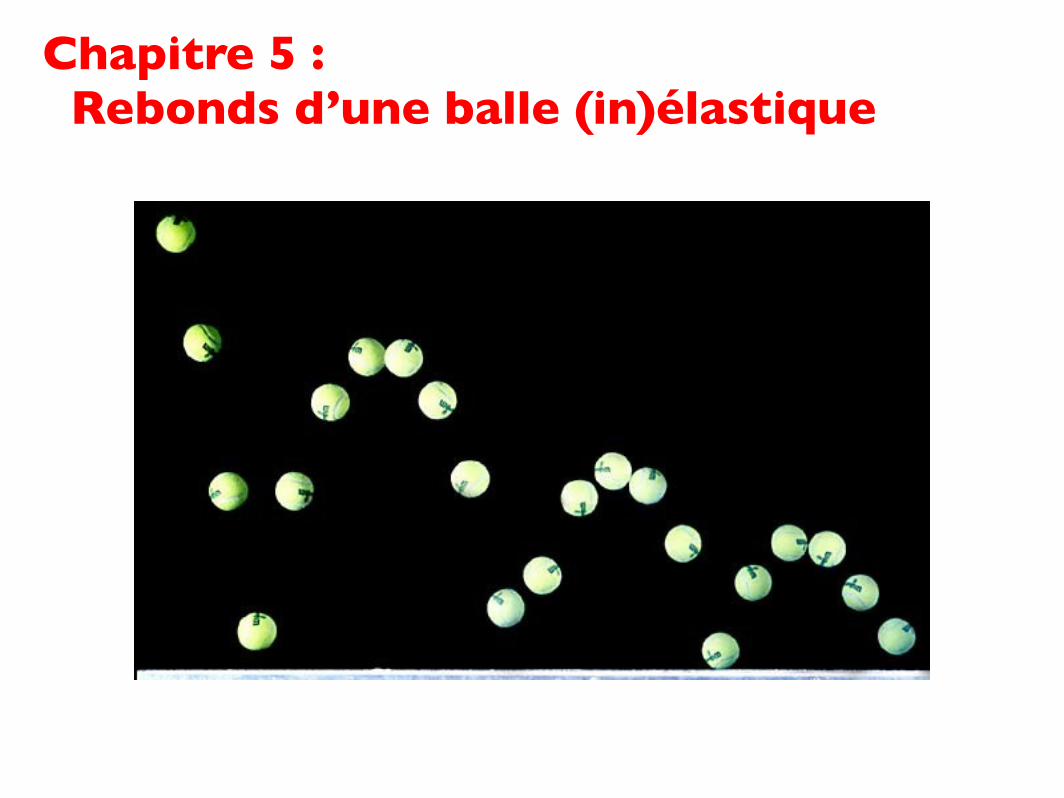
Chapitre 5 : Rebonds d’une balle (in)élastique

Objectifs du chapitre

> Analyser un problème concret

> Systèmes vibrés en physique

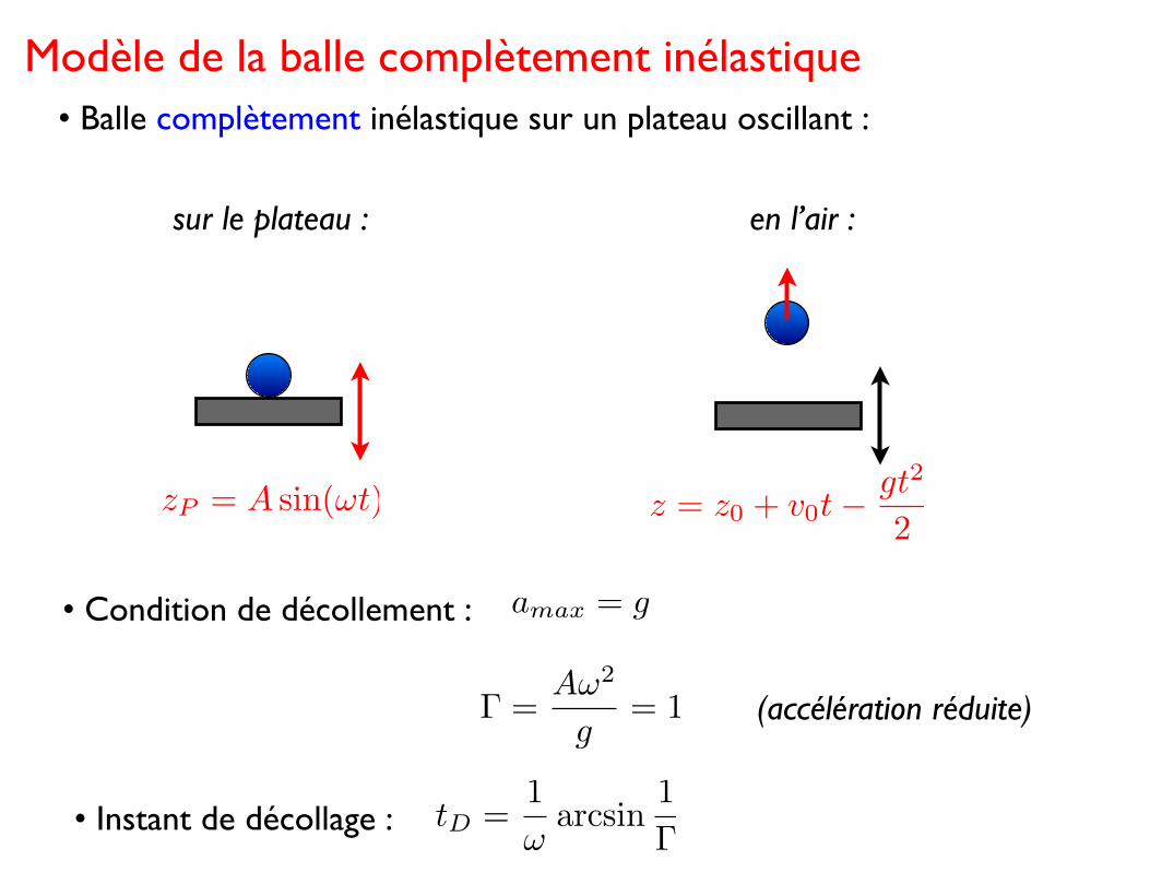
Modèle de la balle complètement inélastique• Balle complètement inélastique sur un plateau oscillant :

sur le plateau : en l’air :

zP = A sin(ωt) z = z0 + v0t−gt2

2

• Condition de décollement : amax = g

Γ =Aω2

g= 1 (accélération réduite)

• Instant de décollage : tD =1ω

arcsin1Γ

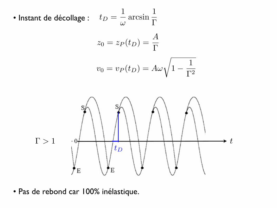
• Instant de décollage : tD =1ω

arcsin1Γ

z0 = zP (tD) =A

Γ

v0 = vP (tD) = Aω

�1− 1

Γ2

ttD

• Pas de rebond car 100% inélastique.

Γ > 1

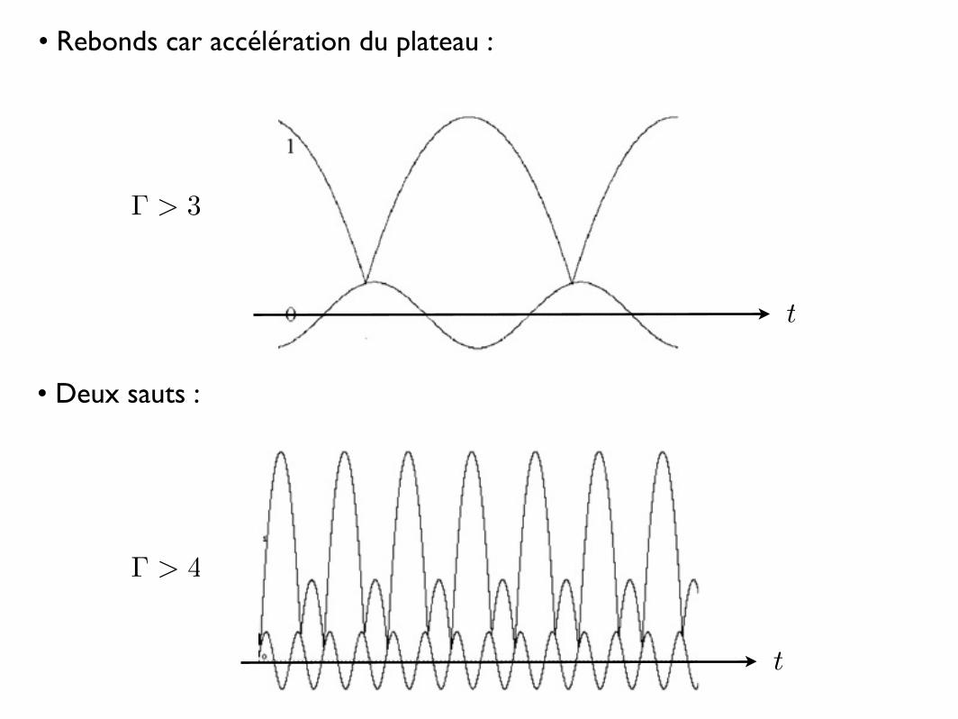
• Rebonds car accélération du plateau :

t

• Deux sauts :

t

Γ > 3

Γ > 4

t

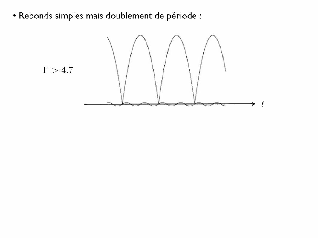
Γ > 4.7

• Rebonds simples mais doublement de période :

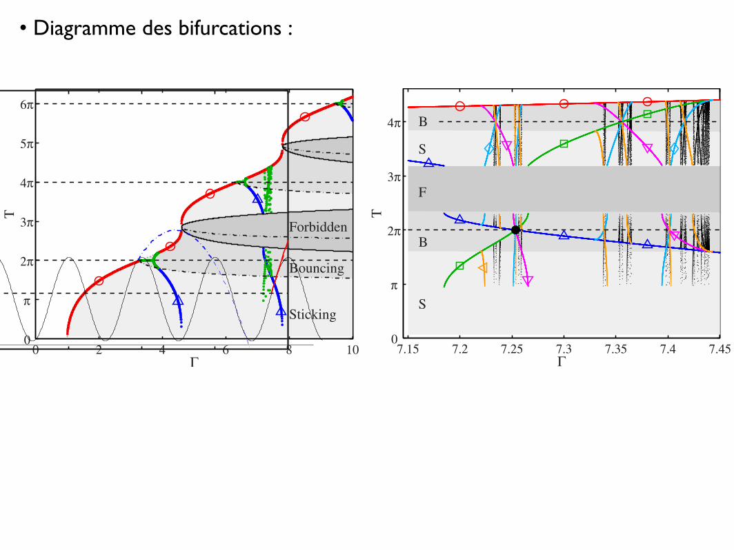
• Diagramme des bifurcations :

ways have two solutions. Only one of them is in the! cos "0#1 zone and is therefore physically relevant. Inother words, there is always one and only one physical solu-tion "0 corresponding to a point in the !! ,T" diagram whichsatisfies !#!1!T"; this diagram contains all the informationnecessary to describe the motion.

For each different successive flight i, the computed flighttime is reported on the !! ,T" diagram, where it forms abranch Bi as a function of ! !Fig. 2". As expected, all thesolutions are located below or on the curve !=!1!T", whichmainly coincides with the branch B1 except around T=2$N,

N!N as explained later. The branch B2!%" decreases fromB1 to zero. More than two branches are observed around !#7.3. In the following, three kind of zones !bouncing, stick-ing, and forbidden" are identified in the diagram, delimitedby curves !BS!T", !FB!T", and !SF!T". A branch that switchesfrom a zone to another is related to a specific bifurcation ofthe system.

The bouncing zone corresponds to flights T that impact ata phase "i="0+T such as ! cos "i#1, which is equivalentto !#!BS!T",

!BS2 =

$1 +T2

2%2

! 2$1 +T2

2%!T sin T + cos T" + T2 ! 1

!sin T ! T cos T"2 .

!5"

Since it may be shown that d!BS /dT has the same sign as!1!! cos "0", only the decreasing part of !BS is relevant as aseparation between bouncing and sticking !Fig. 2". As seenin Fig. 3, a period-doubling bifurcation occurs when a branchcrosses the !BS curve from sticking to bouncing.

For some given accelerations, there is a range of flighttimes that cannot be experienced, as easily understood byinspecting Fig. 4. The parabolic trajectory may be tangent tothe forcing sinusoid, which means that the ball smoothlylands on the vibrated plate at tangent point M. Trajectoriesthat lay above skip this landing opportunity and impact later!after point O". On the other hand, trajectories that lay belowimpact and bounce before M and have a relatively shortflight time T. This discontinuity in T is mainly due to thepossibility for the free-flight parabola to intercept the forcingsinusoid in more than one point !only the first intersectionwould correspond to a physically relevant impact". This to-pological transition is similar to the common tangent bifur-cation, which here results in incrementing or decrementingthe number of flights by one. The flight time at point M isgiven by !=!FB!T", where

0 2! 4! 6! 8! 10! 12!"5

0

5

10

!

x(!)

FIG. 1. !Color online" A plate is vibrated sinusoidally accordingto xp=! cos " !shaded". The solid line is the trajectory x!"" of acompletely inelastic ball let on this plate when !=4. The red !re-spectively, blue" part corresponds to the first !respectively, second"flight. The successive take-off phases "0 and impact phases !"0+T" are represented by !!" and !!", respectively. The dashed hori-zontal line xp=! cos "=1 separates the bouncing and stickingzones.

0 2 4 6 8 100

!

2!

3!

4!

5!

6!

Sticking

Bouncing

Forbidden

"

T

FIG. 2. !Color online" !! ,T" diagram. Shadings indicate thedifferent zones !bouncing, sticking, and forbidden", while coloredsymbol lines correspond to the branches Bi of flight i obtained bysolving Eq. !2" numerically: !!" B1, !"" B2, !!" B3, and next ones.The dashed curve corresponds to !1!T", the decreasing solid curvecorresponds to !FB!T", the increasing solid curve corresponds to!SF, and the decreasing solid curve corresponds to !BS. The dottedlines indicate fixed points in T=2$N, with N!N.

0 4! 8! 12! 16! 20! 24!"1

0

1

2

3

4

5

!

x/#

FIG. 3. !Color online" Period-doubling bifurcation. The solidtrajectory !!=7.320" sticks after three flights while the dash-dottrajectory !!=7.336" experiences five bounces before sticking at thesixth flight. Notations are the same as in Fig. 1.

GILET, VANDEWALLE, AND DORBOLO PHYSICAL REVIEW E 79, 055201!R" !2009"

RAPID COMMUNICATIONS

055201-2!FB =T

2!sin2T

2! . "6#

As for Eq. "5#, only the decreasing part of !FB"T# is physi-cally relevant "Fig. 2#. The other bound of the forbiddenregion !SF"T# is given by point O in Fig. 4, for which theposition may be obtained numerically by solving Eq. "2# for!=!FB. We note that there is another possibility for the pa-rabola to be tangent to the sinusoid, i.e., at point N given byT /2=tan T /2, !!. Nevertheless, this second tangent pointcannot be reached physically.

As mentioned previously, there are some trajectories thatnever enter the sticking region. Nevertheless, those trajecto-ries quickly converge to a periodic bouncing motion similarto the one encountered in the partially elastic ball $1%. Aperiod-1 motion is obtained for T=2"N and ! sin #0=!"N,!N!N0. In the "! ,T# diagram "Fig. 2#, the numerical solu-tion leaves the curve !1"T# and experiences a plateau in T=2"N. This fixed point of Eq. "2# exists when !$&1+"2N2. At each bounce, any perturbation from thisequilibrium grows by a factor equal to the Floquet multiplier

d"#0 + T#d#0

= 1 ! &!2 ! "2N2. "7#

Therefore, the solution is stable when ' d"#0+T#d#0

'%1, i.e., until!=&4+"2N2. Period doubling occurs for larger values of !.The upper branch B1 quickly joins the !1 curve, while thelower branch B2 enters the sticking zone at the same time.

A deeper zoom in the range !! $7.15,7.45% of the "! ,T#diagram reveals an intricate structure "Fig. 5# generated bythe successive bifurcations occurring each time a branchchanges of zone. Branches of odd-degree "respectively, even#monotonically increase "decrease# with an increase in !.When a branch crosses one of the horizontal lines T=2"N,

every branch of higher degree should cross the line at thesame accumulation point !S. This is easily understood byinspecting Fig. 6, which corresponds to acceleration veryclose to !S(7.253 378: at first bounce, the ball lands in thevicinity of the unstable fixed point T=2"N. If landing islocated exactly on this point, every further impact shouldoccur at the same phase, which explains the branch crossing.But any small disturbance is amplified and the trajectoryeventually reaches the sticking zone after a finite but arbi-trarily large number of bounces. An infinity of branches hasto be created through an infinity of bifurcations convergingto the accumulation point. A second infinity of bifurcationsannihilates those branches at !&!S. A logarithmic zoom on!S reveals that this cascade of bifurcations is self-similar"Fig. 7#. A complex branch pattern is repeated indefinitelywith a scaling factor of 30.67, different from the Feigenbaumconstant. Inside this pattern, branches are seen to regularly

2! 4! 6! 8! 10!"1

0

1

2

3

4

5

M

NO

!

x/#

FIG. 4. "Color online# Saddle-node bifurcation. The trajectorymay be tangent to the forcing sinusoid in points M and N. The solidtrajectory "!=7.15# just passes point M, impacts in O and sticksafter two flights while the dash-dot trajectory "!=7.20# impactsbefore M and so experiences three flights before sticking. Notationsare the same as in Fig. 1.

7.15 7.2 7.25 7.3 7.35 7.4 7.450

!

2!

3!

4!

S

B

F

S

B

"T

FIG. 5. "Color online# Zoom in the range !! $7.15,7.45% of the"! ,T# diagram. "!# B1, ""# B2, "## B3, "$# B4, "!# B5, "!# B6, and"·# Bi, with i$6. The dashed lines correspond to T=2"N. Thebullet "!# denotes the accumulation point !S(7.253 378, wherebranches Bi, i'2 intersect each others in T=2". Other notationsare the same as in Fig. 2.

0 6! 12! 18! 24! 30! 36!"1

0

1

2

3

4

5

!

x/#

FIG. 6. "Color online# Typical trajectory that occurs whenbranches Bi, i'2 enter into the vicinity of the unstable fixed pointT=2". Notations are the same as in Fig. 1.

COMPLETELY INELASTIC BALL PHYSICAL REVIEW E 79, 055201"R# "2009#

RAPID COMMUNICATIONS

055201-3

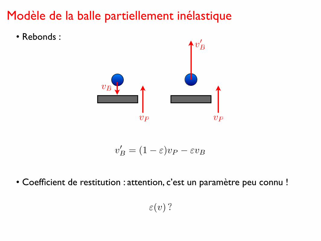
Modèle de la balle partiellement inélastique

• Rebonds :

vP vP

vB

v�B

• Coefficient de restitution : attention, c’est un paramètre peu connu !

v�B = (1− ε)vP − εvB

ε(v) ?

τ

Γ

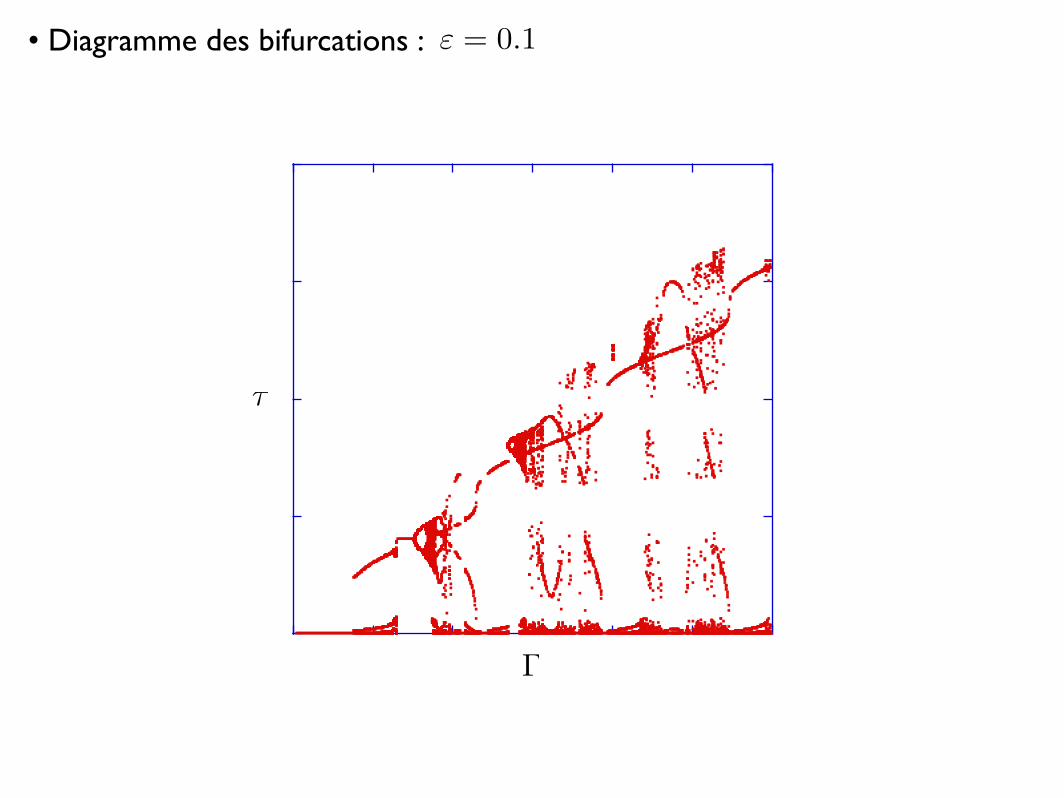
• Diagramme des bifurcations : ε = 0.1

τ

Γ

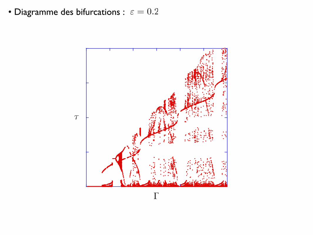
• Diagramme des bifurcations : ε = 0.2

τ

Γ

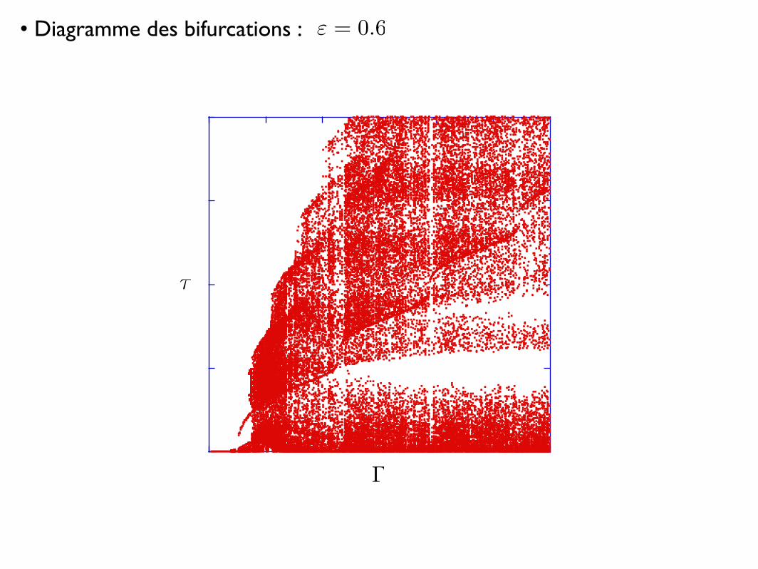
• Diagramme des bifurcations : ε = 0.6

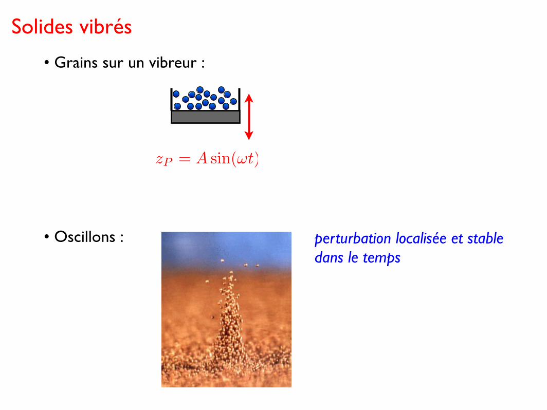
Solides vibrés

• Oscillons :

• Grains sur un vibreur :

zP = A sin(ωt)

perturbation localisée et stable dans le temps

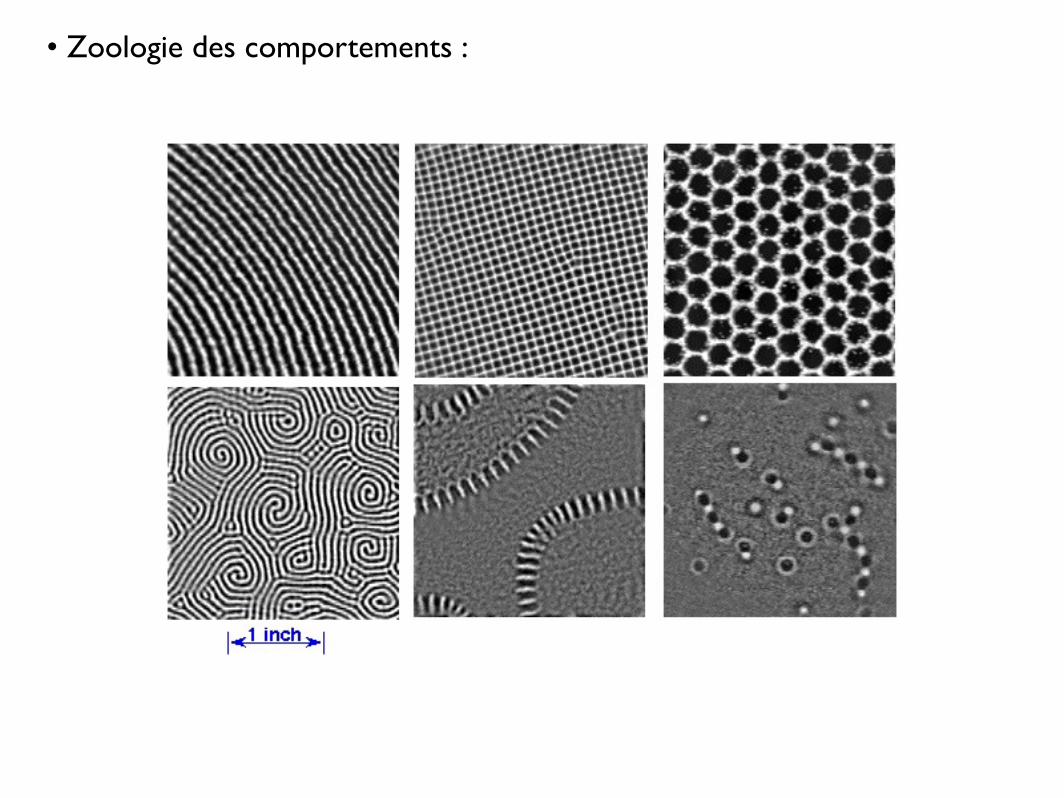
• Zoologie des comportements :

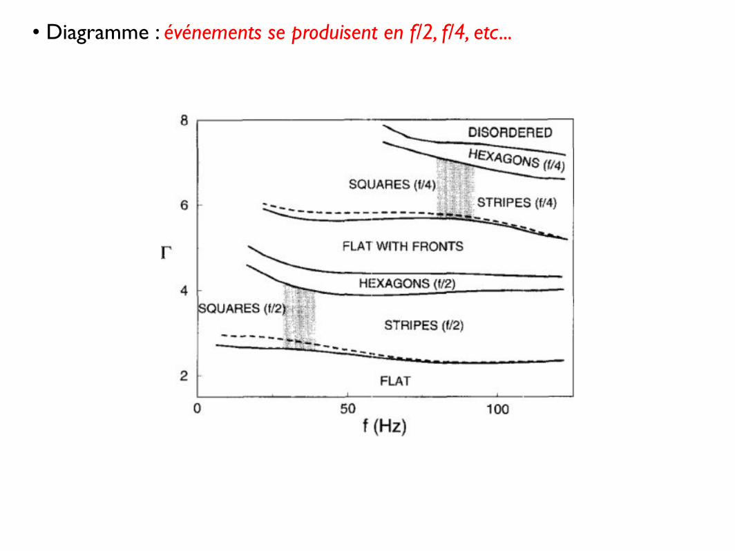
• Diagramme : événements se produisent en f/2, f/4, etc...

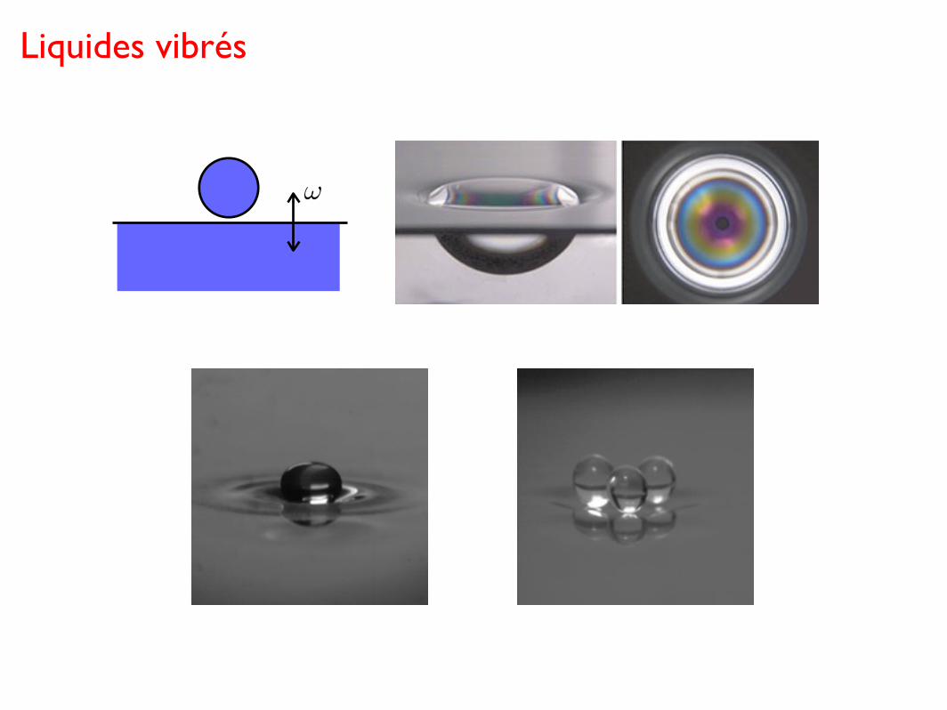
Liquides vibrés

!

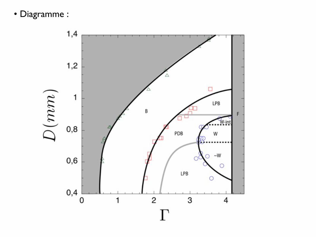
• Diagramme :

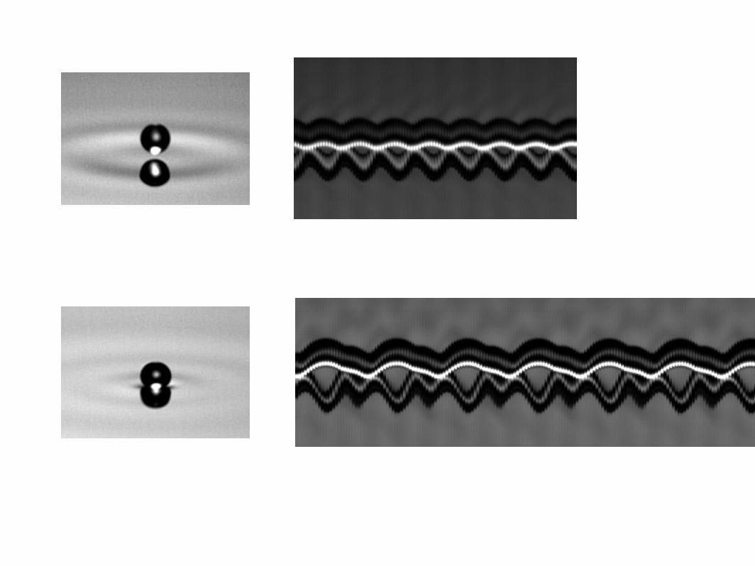
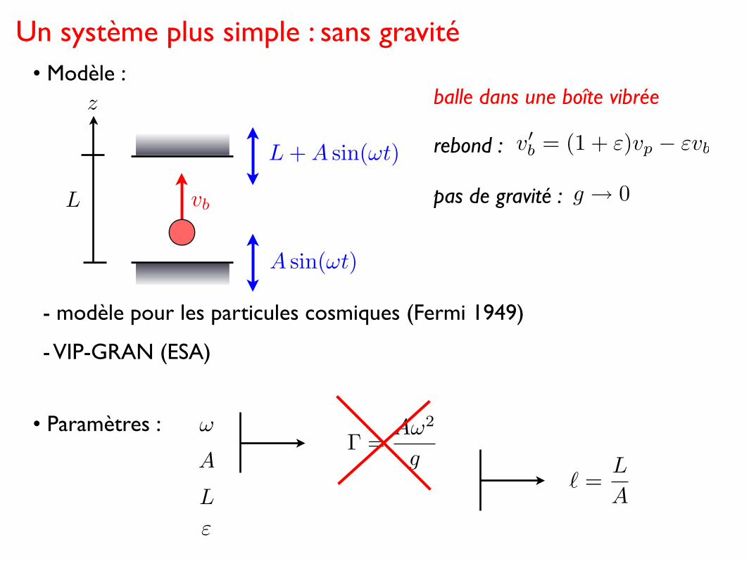
Un système plus simple : sans gravité

balle dans une boîte vibrée

rebond :

pas de gravité : g → 0

v�b = (1 + ε)vp − εvb

L

z

L + A sin(ωt)

A sin(ωt)

vb

- modèle pour les particules cosmiques (Fermi 1949)

- VIP-GRAN (ESA)

ω

A

ε

L

Γ =Aω2

g� =

L

A

• Modèle :

• Paramètres :

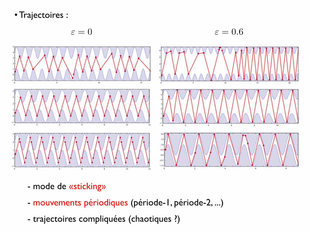
ε = 0 ε = 0.6

- mode de «sticking»

- mouvements périodiques (période-1, période-2, ...)

- trajectoires compliquées (chaotiques ?)

• Trajectoires :

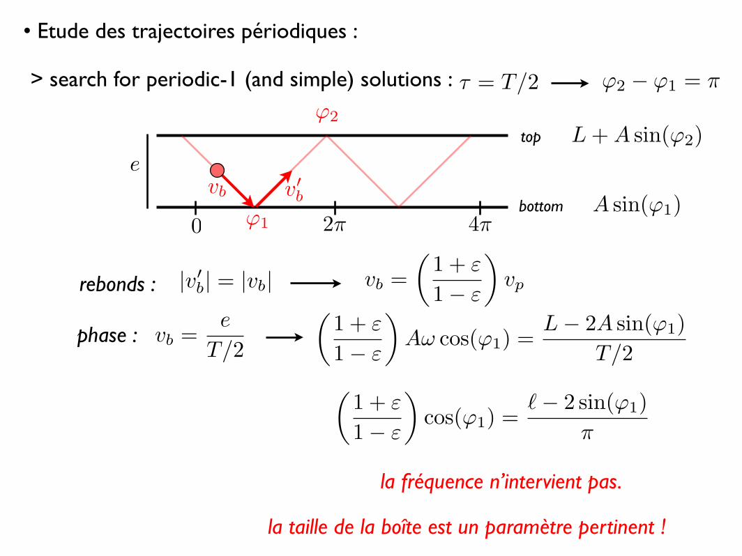
la fréquence n’intervient pas.

> search for periodic-1 (and simple) solutions :

rebonds :

phase :

|v�b| = |vb| vb =

�1 + ε

1− ε

�vp

vb v�b

0 2π 4π

e

ϕ1

ϕ2top

bottom

τ = T/2 ϕ2 − ϕ1 = π

vb =e

T/2

L + A sin(ϕ2)

A sin(ϕ1)

�1 + ε

1− ε

�Aω cos(ϕ1) =

L− 2A sin(ϕ1)T/2

�1 + ε

1− ε

�cos(ϕ1) =

�− 2 sin(ϕ1)π

la taille de la boîte est un paramètre pertinent !

• Etude des trajectoires périodiques :

�

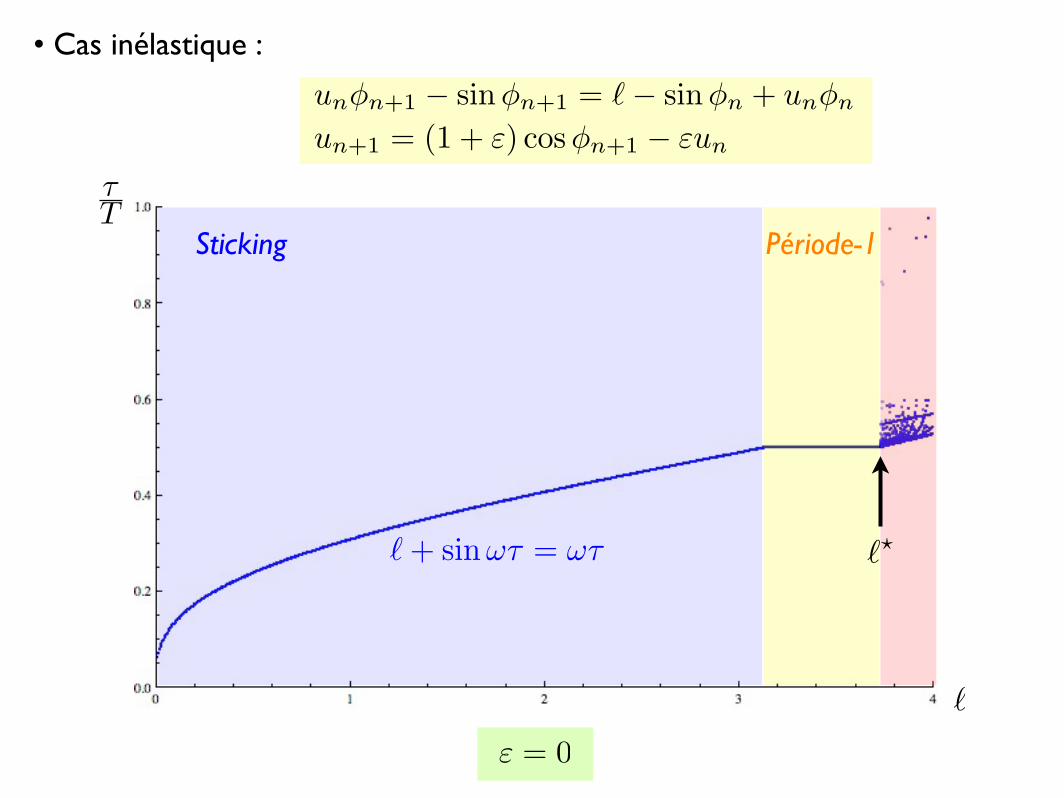
τT

ε = 0

��

Sticking Période-1

� + sinωτ = ωτ

• Cas inélastique :

unφn+1 − sinφn+1 = �− sinφn + unφn

un+1 = (1 + ε) cos φn+1 − εun

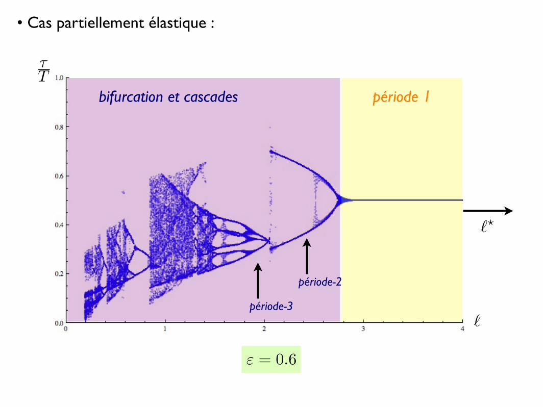
ε = 0.6

��

�

τT

période 1bifurcation et cascades

période-2

période-3

• Cas partiellement élastique :

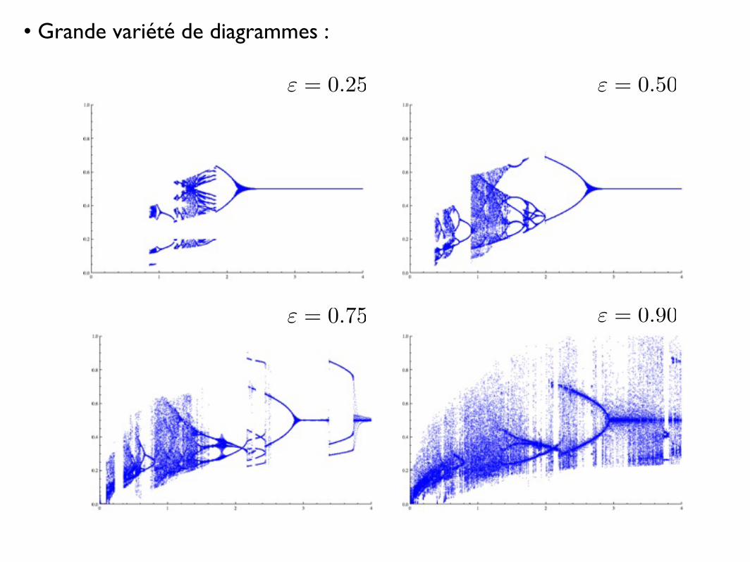
ε = 0.25 ε = 0.50

ε = 0.75 ε = 0.90

• Grande variété de diagrammes :

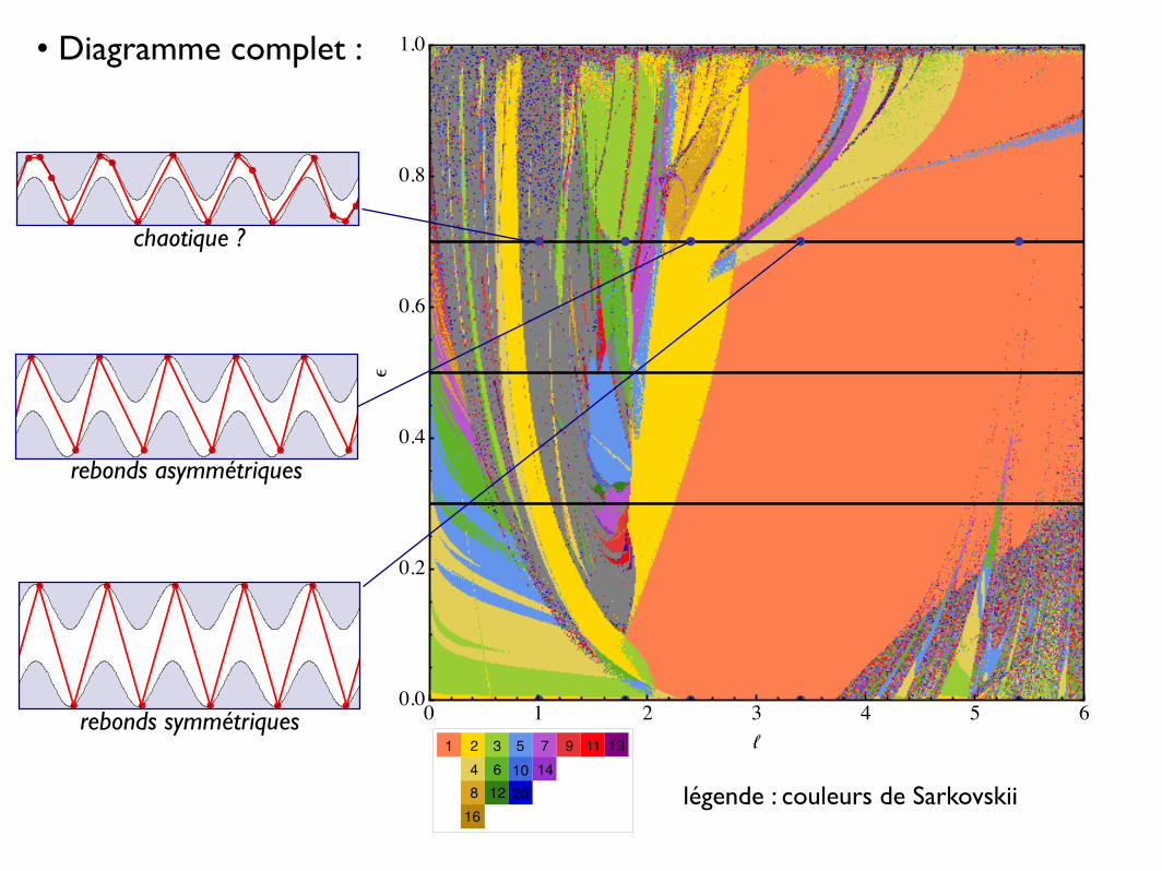
• Diagramme complet :

0 1 2 3 4 5 60.0

0.2

0.4

0.6

0.8

1.0

�

Ε

1 2 3 5 7 9 11 134816

612

1020

14

légende : couleurs de Sarkovskii

rebonds symmétriques

rebonds asymmétriques

chaotique ?

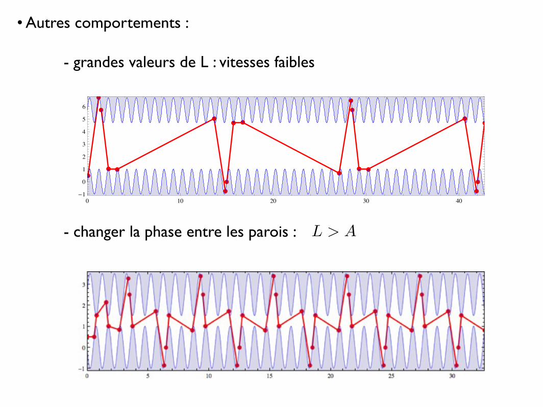
- grandes valeurs de L : vitesses faibles

- changer la phase entre les parois : L > A

0 10 20 30 40�1

0

1

2

3

4

5

6

• Autres comportements :