Oscillatory and Competition Instabilities: Dynamics of ...ward/papers/nonwaves.pdf · Dynamic...

Oscillatory and Competition Instabilities:Dynamics of Spikes for the Gray-Scott

ModelWentao Sun (Mitacs Postdoc, U. Calgary)

Jens Rademacher (CWI, Amsterdam)Chen Wan, Michael Ward (UBC)

[email protected]

Seattle, September 2006 – p.1

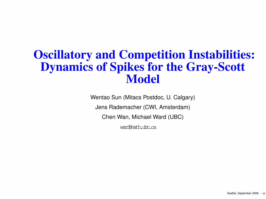
Singularly Perturbed RD ModelsSpatially localized solutions occur for RD models of the form:

vt = ε24v + g(u, v) ; τut = D4u + f(u, v) , ∂nu = ∂nv = 0 x ∈ ∂Ω .

Since ε 1, then v is localized as a spike (1-D) or a spot (2-D). There aretwo well-known choices:

Classic Gierer-Meinhardt Model (1972):

g(u, v) = −v + v2/u f(u, v) = −u + v2 .

Simplest in a hierarchy of more complicated models (morphogenesis,patterns on sea-shells etc.)Gray-Scott Model (1988):

g(u, v) = −v + Auv2 , f(u, v) = (1 − u) − uv2 .

Chemical patterns in a continuously fed reactor. Intricate patternsdepending on D and A (Pearson 1993, Swinney et al. 1993, Nishiuraet al., Doleman et al., Muratov and Osipov, KWW).


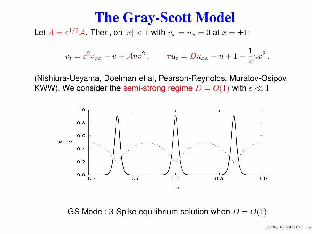
The Gray-Scott ModelLet A = ε1/2A. Then, on |x| < 1 with vx = ux = 0 at x = ±1:

vt = ε2vxx − v + Auv2 , τut = Duxx − u + 1 − 1

εuv2 .

(Nishiura-Ueyama, Doelman et al, Pearson-Reynolds, Muratov-Osipov,KWW). We consider the semi-strong regime D = O(1) with ε 1

GS Model: 3-Spike equilibrium solution when D = O(1)


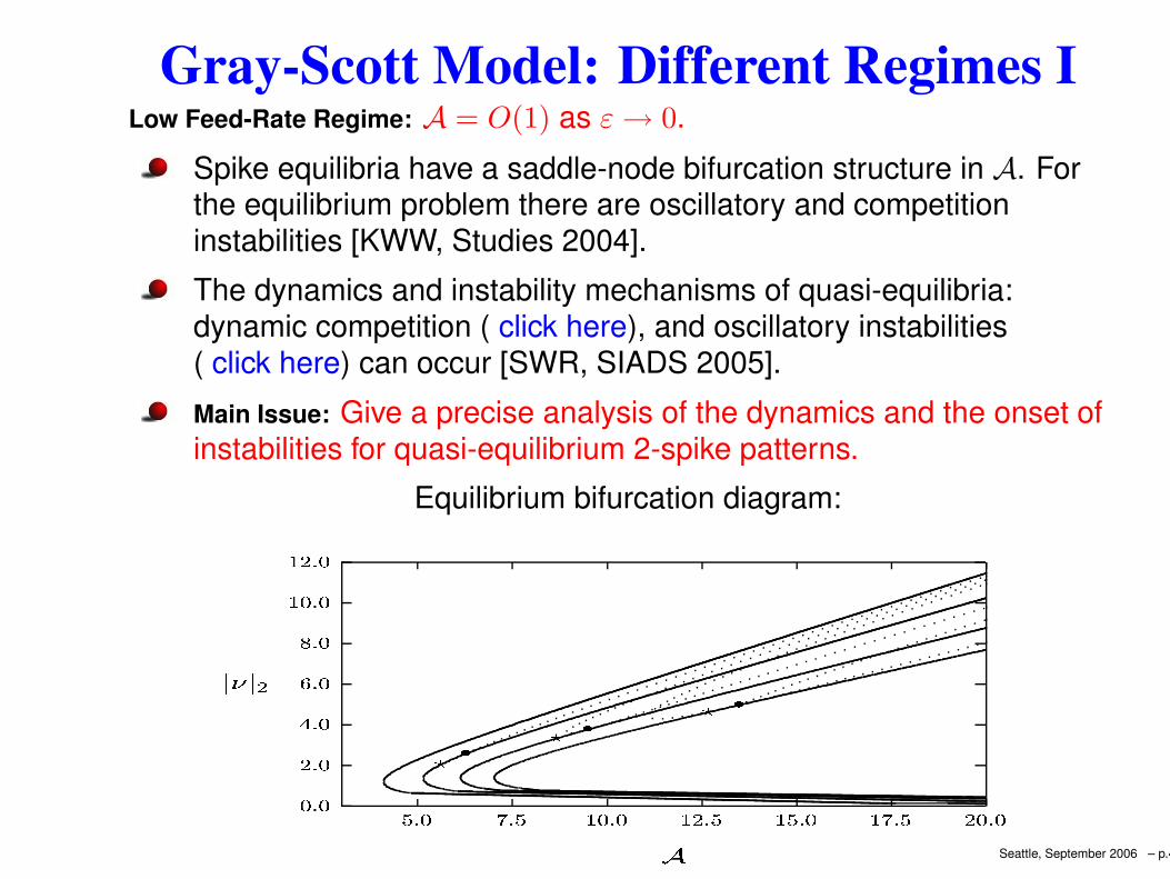
Gray-Scott Model: Different Regimes ILow Feed-Rate Regime: A = O(1) as ε → 0.

Spike equilibria have a saddle-node bifurcation structure in A. Forthe equilibrium problem there are oscillatory and competitioninstabilities [KWW, Studies 2004].The dynamics and instability mechanisms of quasi-equilibria:dynamic competition ( click here), and oscillatory instabilities( click here) can occur [SWR, SIADS 2005].Main Issue: Give a precise analysis of the dynamics and the onset ofinstabilities for quasi-equilibrium 2-spike patterns.

Equilibrium bifurcation diagram:


The Gray-Scott Model: Different Regimes IIIntermediate Regime: O(1) A O(ε−1/2).

Dynamics and NLEP stability of 2-spike quasi-equilibria onunbounded domains (Doelman et al. SIADS 2003)For N -spike patterns on a bounded domain, static oscillatory profileinstabilities for O(1) A O(ε−1/3) with τH = O(A4) are analyzedfrom a universal one-multiplier NLEP. (W. Chen, MJW)On a bounded domain, for O(ε−1/3) A O(ε−1/2) oscillatory driftinstabilities dominate since τTW = O(ε−2A−2) τH . (Doelman et al,Muratov-Osipov, KWW). Large-scale oscillatory spike motion fromtime-dependent heat equation (W. Chen, MJW).

High-Feed Regime: A = O(ε−1/2).A “core problem” determines the spike profile (Doelman et al,Muratov-Osipov, KWW). Intricate bifurcation structure (DKP, 2006)Instability mechanism is oscillatory drift instability on a finite domainwhen τ = τTW = O(ε−1) [KWW, Physica D 2004).Simulataneous pulse-splitting can occur. Core problem coupled to atime-dependent PDE when τ = O(ε−1).


Comparison of Two Slow Processes: IDynamics of Quasi-Equilibria: Cahn-Hilliard, Allen-Cahn:

ut = ε2uxx + u − u3 , (AC) ; ut = −(ε2uxx + u − u3)xx , (CH) .

Metastable dynamics for widely-spaced heteroclinic layers. Theevolution occurs over exponentially long time intervals in 1-D.Coarsening Process: Collapse events punctuate the metastabledynamics in 1-D. K-layer solutions cascade to K − 2 layer solutionsfrom pairwise collapse of nearest neighbours. The collapse processis local in space and time. The quasi-equilibrium profile for widelyspaced layers is unconditionally stable.Variational Structure and Gradient Flow: the final equilibrium state of nointerfaces (Allen-Cahn), or one interface from mass conservation(Cahn-Hilliard) is a minimum energy solution.

Weakly Interacting (Metastable) Pulses: Tail interactions of exponentially local-

ized pulses determine the dynamics (Ei, Sandstede...).


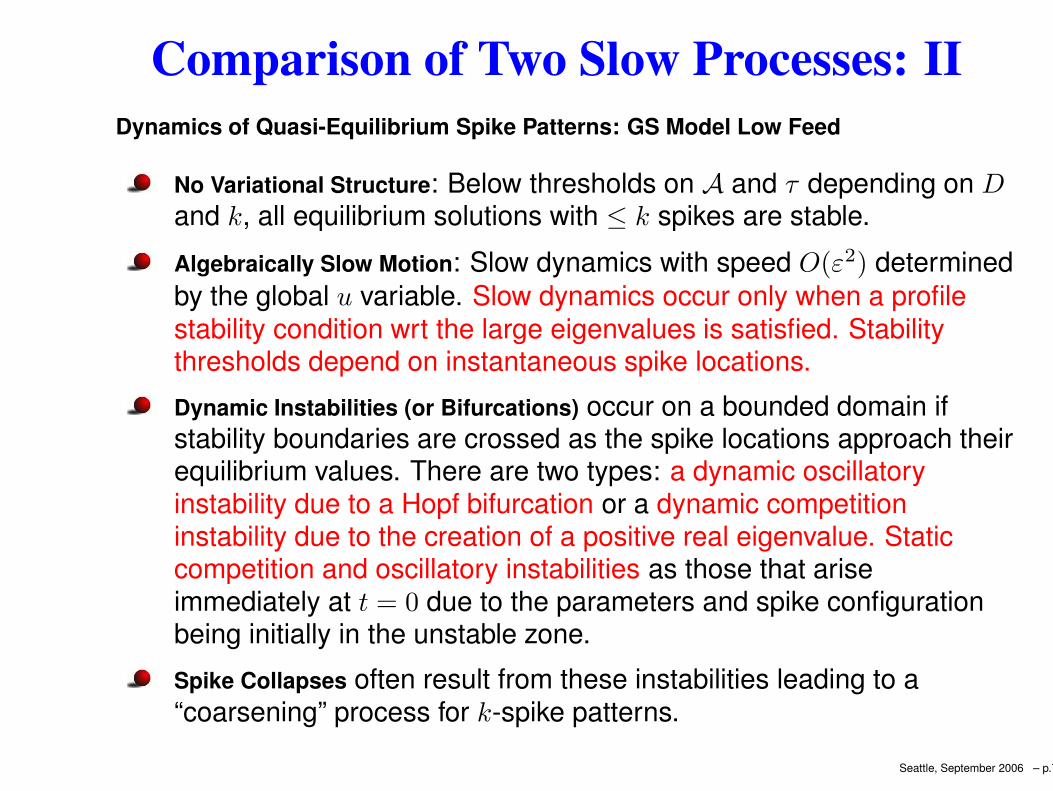
Comparison of Two Slow Processes: IIDynamics of Quasi-Equilibrium Spike Patterns: GS Model Low Feed

No Variational Structure: Below thresholds on A and τ depending on Dand k, all equilibrium solutions with ≤ k spikes are stable.Algebraically Slow Motion: Slow dynamics with speed O(ε2) determinedby the global u variable. Slow dynamics occur only when a profilestability condition wrt the large eigenvalues is satisfied. Stabilitythresholds depend on instantaneous spike locations.Dynamic Instabilities (or Bifurcations) occur on a bounded domain ifstability boundaries are crossed as the spike locations approach theirequilibrium values. There are two types: a dynamic oscillatoryinstability due to a Hopf bifurcation or a dynamic competitioninstability due to the creation of a positive real eigenvalue. Staticcompetition and oscillatory instabilities as those that ariseimmediately at t = 0 due to the parameters and spike configurationbeing initially in the unstable zone.Spike Collapses often result from these instabilities leading to a“coarsening” process for k-spike patterns.


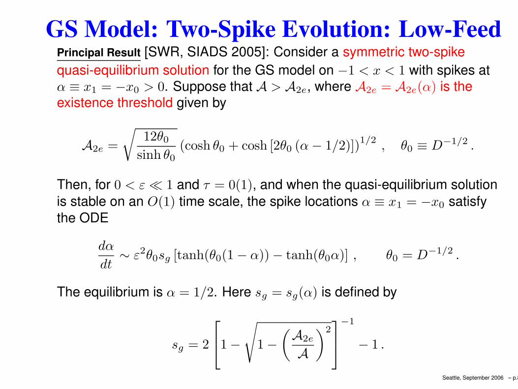
GS Model: Two-Spike Evolution: Low-FeedPrincipal Result [SWR, SIADS 2005]: Consider a symmetric two-spikequasi-equilibrium solution for the GS model on −1 < x < 1 with spikes atα ≡ x1 = −x0 > 0. Suppose that A > A2e, where A2e = A2e(α) is theexistence threshold given by

A2e =

√

12θ0

sinh θ0

(cosh θ0 + cosh [2θ0 (α − 1/2)])1/2 , θ0 ≡ D−1/2 .

Then, for 0 < ε 1 and τ = 0(1), and when the quasi-equilibrium solutionis stable on an O(1) time scale, the spike locations α ≡ x1 = −x0 satisfythe ODE

dα

dt∼ ε2θ0sg [tanh(θ0(1 − α)) − tanh(θ0α)] , θ0 = D−1/2 .

The equilibrium is α = 1/2. Here sg = sg(α) is defined by

sg = 2

1 −

√

1 −(A2e

A

)2

−1

− 1 .


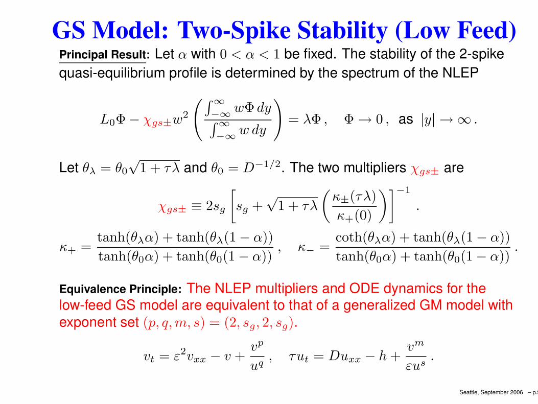
GS Model: Two-Spike Stability (Low Feed)Principal Result: Let α with 0 < α < 1 be fixed. The stability of the 2-spikequasi-equilibrium profile is determined by the spectrum of the NLEP

L0Φ − χgs±w2

(∫∞−∞ wΦ dy∫∞−∞ w dy

)

= λΦ , Φ → 0 , as |y| → ∞ .

Let θλ = θ0

√1 + τλ and θ0 = D−1/2. The two multipliers χgs± are

χgs± ≡ 2sg

[

sg +√

1 + τλ

(

κ±(τλ)

κ+(0)

)]−1

.

κ+ =tanh(θλα) + tanh(θλ(1 − α))

tanh(θ0α) + tanh(θ0(1 − α)), κ− =

coth(θλα) + tanh(θλ(1 − α))

tanh(θ0α) + tanh(θ0(1 − α)).

Equivalence Principle: The NLEP multipliers and ODE dynamics for thelow-feed GS model are equivalent to that of a generalized GM model withexponent set (p, q, m, s) = (2, sg, 2, sg).

vt = ε2vxx − v +vp

uq, τut = Duxx − h +

vm

εus.


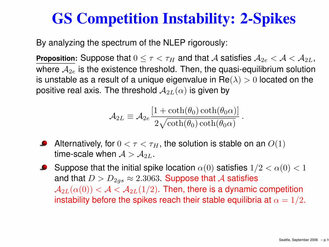
GS Competition Instability: 2-SpikesBy analyzing the spectrum of the NLEP rigorously:Proposition: Suppose that 0 ≤ τ < τH and that A satisfies A2e < A < A2L,where A2e is the existence threshold. Then, the quasi-equilibrium solutionis unstable as a result of a unique eigenvalue in Re(λ) > 0 located on thepositive real axis. The threshold A2L(α) is given by

A2L ≡ A2e[1 + coth(θ0) coth(θ0α)]

2√

coth(θ0) coth(θ0α).

Alternatively, for 0 < τ < τH , the solution is stable on an O(1)time-scale when A > A2L.Suppose that the initial spike location α(0) satisfies 1/2 < α(0) < 1and that D > D2gs ≈ 2.3063. Suppose that A satisfiesA2L(α(0)) < A < A2L(1/2). Then, there is a dynamic competitioninstability before the spikes reach their stable equilibria at α = 1/2.


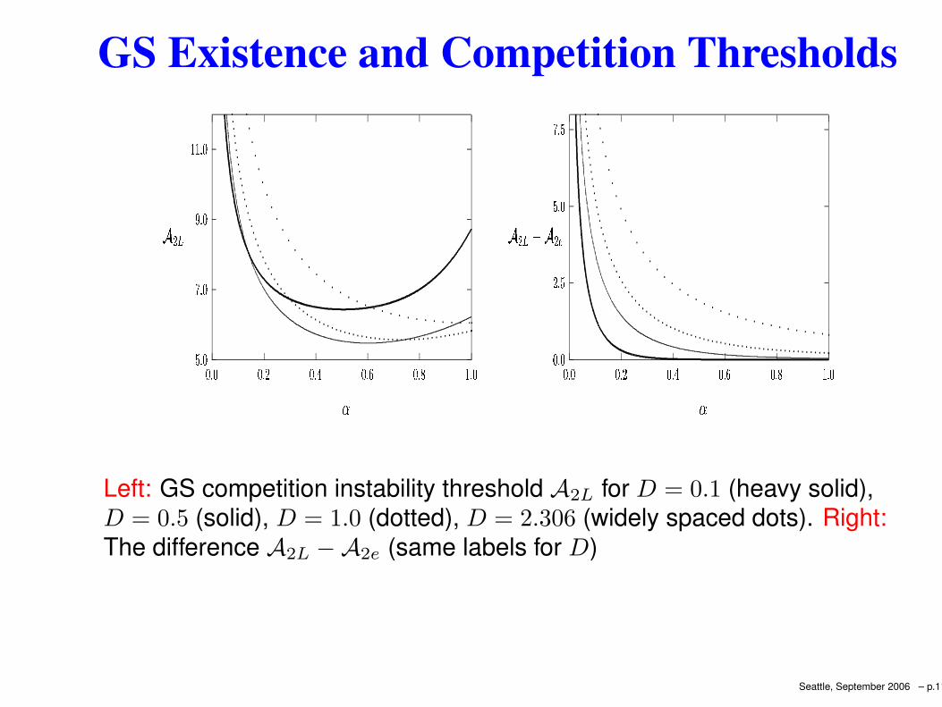
GS Existence and Competition Thresholds

"! #$! #

%"! #& & ! #

#! # #! ' #! ( #! ) #! * & ! #

+-, .

/

0"1 02 1 3

3 1 041 3

01 0 01 2 0"1 5 0"1 6 01 7 8 1 0

9-: ;< 9 :>=

?

Left: GS competition instability threshold A2L for D = 0.1 (heavy solid),D = 0.5 (solid), D = 1.0 (dotted), D = 2.306 (widely spaced dots). Right:The difference A2L −A2e (same labels for D)


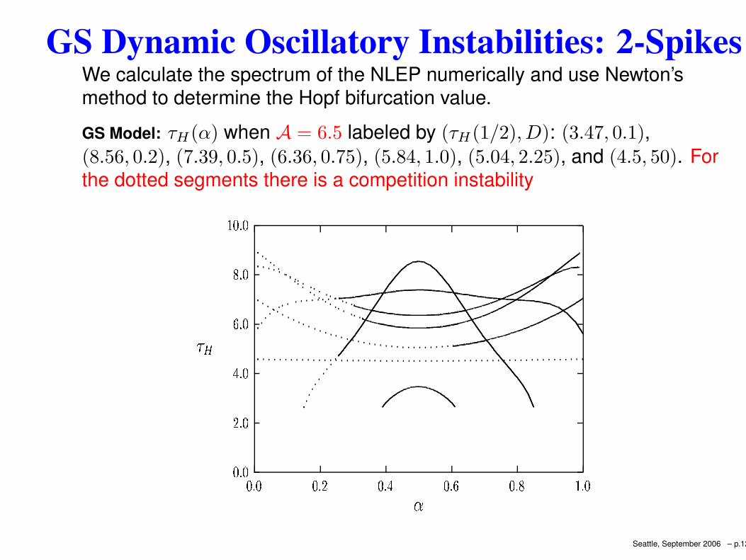
GS Dynamic Oscillatory Instabilities: 2-SpikesWe calculate the spectrum of the NLEP numerically and use Newton’smethod to determine the Hopf bifurcation value.GS Model: τH(α) when A = 6.5 labeled by (τH(1/2), D): (3.47, 0.1),(8.56, 0.2), (7.39, 0.5), (6.36, 0.75), (5.84, 1.0), (5.04, 2.25), and (4.5, 50). Forthe dotted segments there is a competition instability

@BA @C A @

DA @E A @

F A @G @BA @

@A @ @A C @A D @BA E @BA F G A @

HI

J


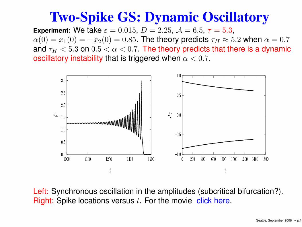
Two-Spike GS: Dynamic OscillatoryExperiment: We take ε = 0.015, D = 2.25, A = 6.5, τ = 5.3,α(0) = x1(0) = −x2(0) = 0.85. The theory predicts τH ≈ 5.2 when α = 0.7and τH < 5.3 on 0.5 < α < 0.7. The theory predicts that there is a dynamicoscillatory instability that is triggered when α < 0.7.

K"L KK"L M

N L KN L M

O L KO L M

P L KN K K K N N K K N O K K N P K K N Q K K

RTS

U

V W"X YV YX Z

YX YYX Z

W"X YY [ Y Y \ Y Y] Y Y ^ Y Y W Y Y Y W [ Y Y W \ Y Y W] Y Y

_`

a

Left: Synchronous oscillation in the amplitudes (subcritical bifurcation?).Right: Spike locations versus t. For the movie click here.


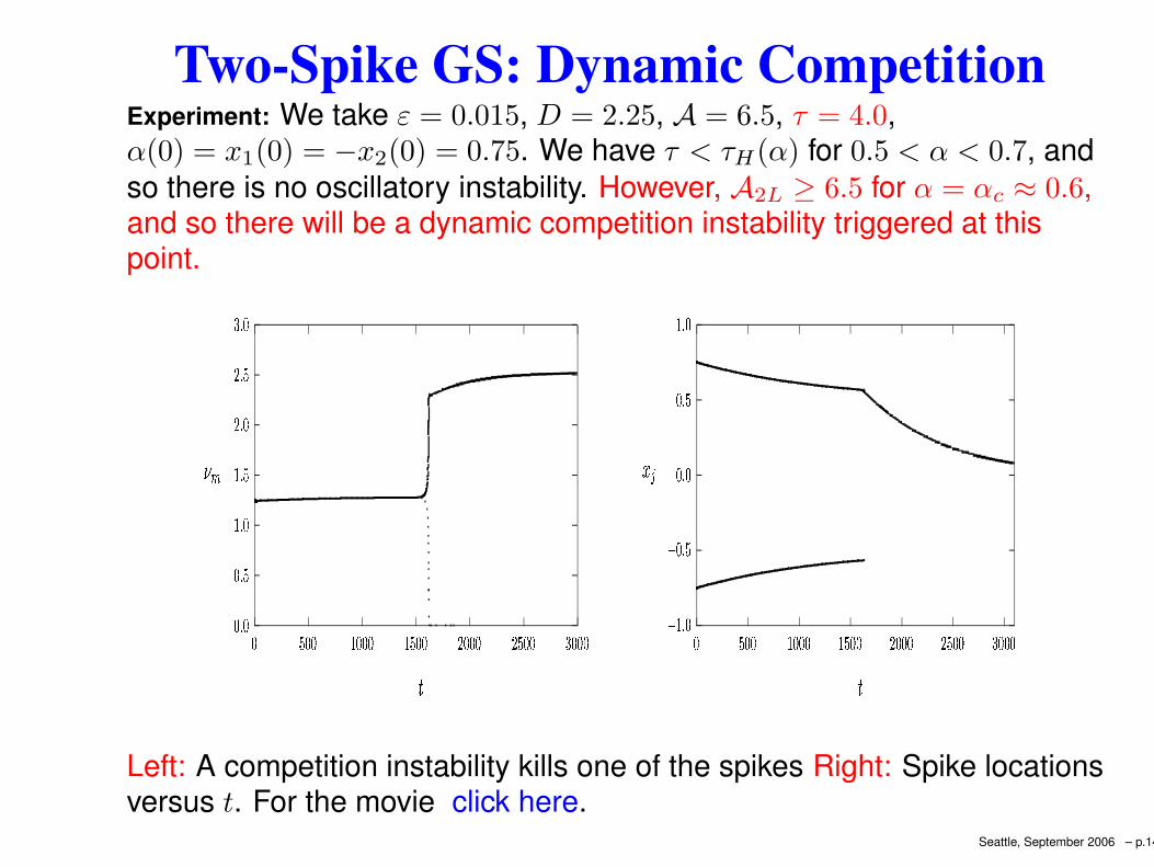
Two-Spike GS: Dynamic CompetitionExperiment: We take ε = 0.015, D = 2.25, A = 6.5, τ = 4.0,α(0) = x1(0) = −x2(0) = 0.75. We have τ < τH(α) for 0.5 < α < 0.7, andso there is no oscillatory instability. However, A2L ≥ 6.5 for α = αc ≈ 0.6,and so there will be a dynamic competition instability triggered at thispoint.

b"c bb"c d

e c be c d

f c bf c d

g c bb d b b e b b b e d b b f b b b f d b b g b b b

hTi

j

k l"m nk nm o

nm nnm o

l"m nn o n n l n n n l o n n p n n n p o n n q n n n

rs

t

Left: A competition instability kills one of the spikes Right: Spike locationsversus t. For the movie click here.


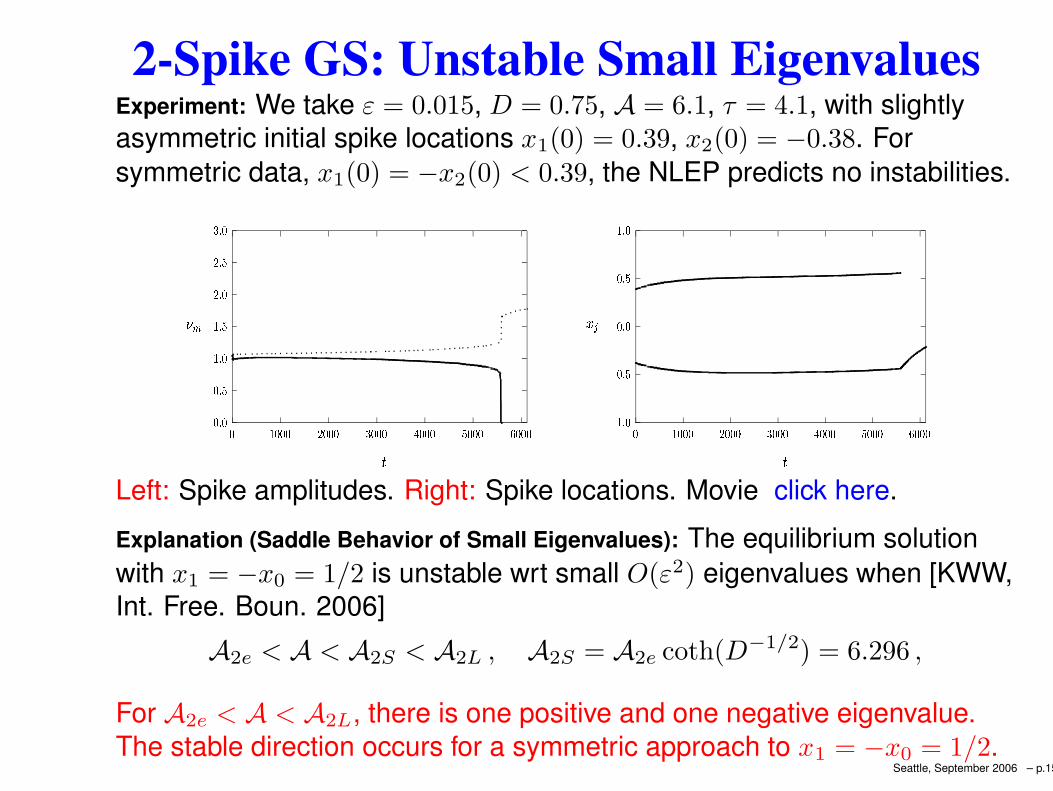
2-Spike GS: Unstable Small EigenvaluesExperiment: We take ε = 0.015, D = 0.75, A = 6.1, τ = 4.1, with slightlyasymmetric initial spike locations x1(0) = 0.39, x2(0) = −0.38. Forsymmetric data, x1(0) = −x2(0) < 0.39, the NLEP predicts no instabilities.

uwv uuwv x

y v uy v x

z v uz v x

v uu y u u u z u u u u u u | u u u x u u u u u u

~

w

w

Left: Spike amplitudes. Right: Spike locations. Movie click here.Explanation (Saddle Behavior of Small Eigenvalues): The equilibrium solutionwith x1 = −x0 = 1/2 is unstable wrt small O(ε2) eigenvalues when [KWW,Int. Free. Boun. 2006]

A2e < A < A2S < A2L , A2S = A2e coth(D−1/2) = 6.296 ,

For A2e < A < A2L, there is one positive and one negative eigenvalue.The stable direction occurs for a symmetric approach to x1 = −x0 = 1/2.


GS Model: Infinite-Domain (Low Feed)Principal Result: Let ε 1 and and consider a quasi-equilibrium two-spikesolution for the GS model with spikes located at αi ≡ x1 = −x0 > 0.Suppose that Ai > A∞

2e, where

A∞2e =

√12(

1 + e−2αi

)1/2,

and that this solution is stable on an O(1) time-scale. Then,

dαi

dt∼ 2ε2

i sge−2αi

1 + e−2αi

, sg = 2

1 −

√

1 −(A∞

2e

Ai

)2

−1

− 1 .

The stability of this solution is determined by the NLEP

L0Φ − χ∞gs±w2

(∫∞−∞ wΦ dy∫∞−∞ w dy

)

= λΦ , Φ → 0 , as |y| → ∞ .

χ∞gs± ≡ 2sg

[

sg +√

1 + τλ

(

1 + e−2αi

1 ± e−2αi

√1+τλ

)]−1

.


GS Model: Infinite-Domain (Low Feed)Proposition: Suppose that A∞

2e < Ai < A∞2L, where

A∞2L ≡ A∞

2e

[1 + coth(αi)]

2√

coth(αi).

Then, for 0 ≤ τ < τH , the q.e. is unstable from a unique positive realeigenvalue. Alternatively, for 0 < τ < τH , the solution is stable whenAi > A∞

2L. A Hopf Bifurcation occurs at τ = τH .Static Competition Instability: occurs at t = 0 when A∞

2e < Ai < A∞2L for

the initial αi(0). Setting Ai = A∞2L we calculate

αic ≡ 1

2log

(

sg + 1

sg − 1

)

, sg = 2

1 −

√

1 −(A∞

2e

Ai

)2

−1

− 1 .

A static competition instability occurs when 0 < αi(0) < αic.However, since α

′

i(t) > 0 and since A∞2L is monotone decreasing in

αi, there are no dynamic competition instabilities.Static Oscillatory Instability: Occurs when αi(0) > αic and τ > τH .Since τ

′

H(αi) > 0 there are no dynamic oscillatory instabilities.Seattle, September 2006 – p.17

GS Intermediate Regime: Scaling Law IConsider the subregime O(1) A O(ε−1/3) of the intermediateregime. In this regime, n-spike quasi-equilibria are de-stabililized first by aHopf bifurcation in the spike amplitudes as τ is increased.

Principal Result:[WanW, 2006]: Let ε 1, τ = O(A4), and let σ = ε2A2t bethe slow time-scale. Near the jth spike

v ∼ Aγjw[

ε−1(x − xj)]

, u ∼ 1

A2γj.

The amplitudes γj(σ) and locations xj(σ) satisfy the tridiagonal DAEsystem:

dx

dσ∼ −θ0UPbe , Be ∼ 6θ0u , θ0 = D−1/2 .

Here x ≡ (x1, ..., xn)t, u ≡ (γ1, .., γn)t, and Uij = γiδij.


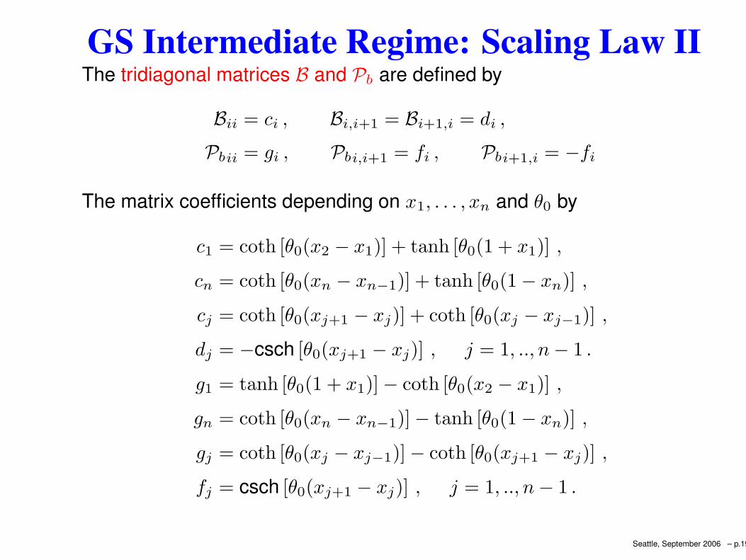
GS Intermediate Regime: Scaling Law IIThe tridiagonal matrices B and Pb are defined by

Bii = ci , Bi,i+1 = Bi+1,i = di ,

Pbii = gi , Pbi,i+1 = fi , Pbi+1,i = −fi

The matrix coefficients depending on x1, . . . , xn and θ0 by

c1 = coth [θ0(x2 − x1)] + tanh [θ0(1 + x1)] ,

cn = coth [θ0(xn − xn−1)] + tanh [θ0(1 − xn)] ,

cj = coth [θ0(xj+1 − xj)] + coth [θ0(xj − xj−1)] ,

dj = −csch [θ0(xj+1 − xj)] , j = 1, .., n − 1 .

g1 = tanh [θ0(1 + x1)] − coth [θ0(x2 − x1)] ,

gn = coth [θ0(xn − xn−1)] − tanh [θ0(1 − xn)] ,

gj = coth [θ0(xj − xj−1)] − coth [θ0(xj+1 − xj)] ,

fj = csch [θ0(xj+1 − xj)] , j = 1, .., n − 1 .


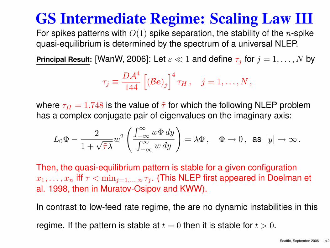
GS Intermediate Regime: Scaling Law IIIFor spikes patterns with O(1) spike separation, the stability of the n-spikequasi-equilibrium is determined by the spectrum of a universal NLEP.Principal Result: [WanW, 2006]: Let ε 1 and define τj for j = 1, . . . , N by

τj ≡ DA4

144

[

(Be)j

]4

τH , j = 1, . . . , N ,

where τH = 1.748 is the value of τ for which the following NLEP problemhas a complex conjugate pair of eigenvalues on the imaginary axis:

L0Φ − 2

1 +√

τλw2

(∫∞−∞ wΦ dy∫∞−∞ w dy

)

= λΦ , Φ → 0 , as |y| → ∞ .

Then, the quasi-equilibrium pattern is stable for a given configurationx1, . . . , xn iff τ < minj=1,...,n τj . (This NLEP first appeared in Doelman etal. 1998, then in Muratov-Osipov and KWW).

In contrast to low-feed rate regime, the are no dynamic instabilities in this

regime. If the pattern is stable at t = 0 then it is stable for t > 0.Seattle, September 2006 – p.20

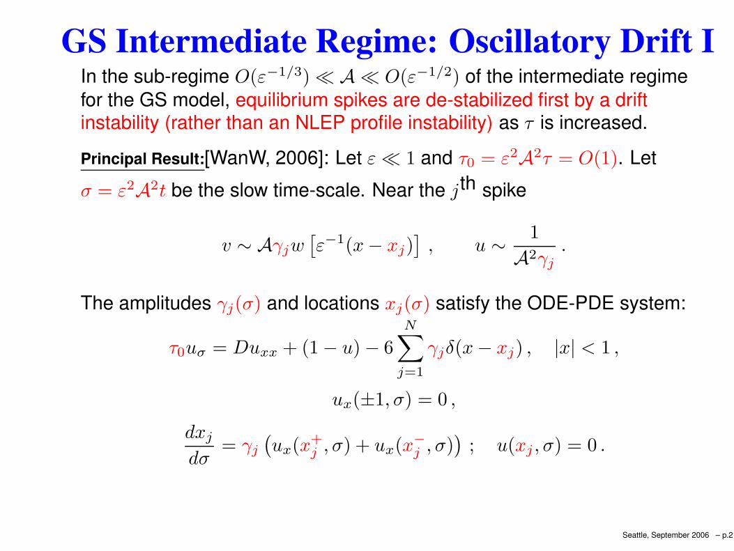
GS Intermediate Regime: Oscillatory Drift IIn the sub-regime O(ε−1/3) A O(ε−1/2) of the intermediate regimefor the GS model, equilibrium spikes are de-stabilized first by a driftinstability (rather than an NLEP profile instability) as τ is increased.Principal Result:[WanW, 2006]: Let ε 1 and τ0 = ε2A2τ = O(1). Letσ = ε2A2t be the slow time-scale. Near the jth spike

v ∼ Aγjw[

ε−1(x − xj)]

, u ∼ 1

A2γj.

The amplitudes γj(σ) and locations xj(σ) satisfy the ODE-PDE system:

τ0uσ = Duxx + (1 − u) − 6N∑

j=1

γjδ(x − xj) , |x| < 1 ,

ux(±1, σ) = 0 ,

dxj

dσ= γj

(

ux(x+

j , σ) + ux(x−j , σ)

)

; u(xj , σ) = 0 .


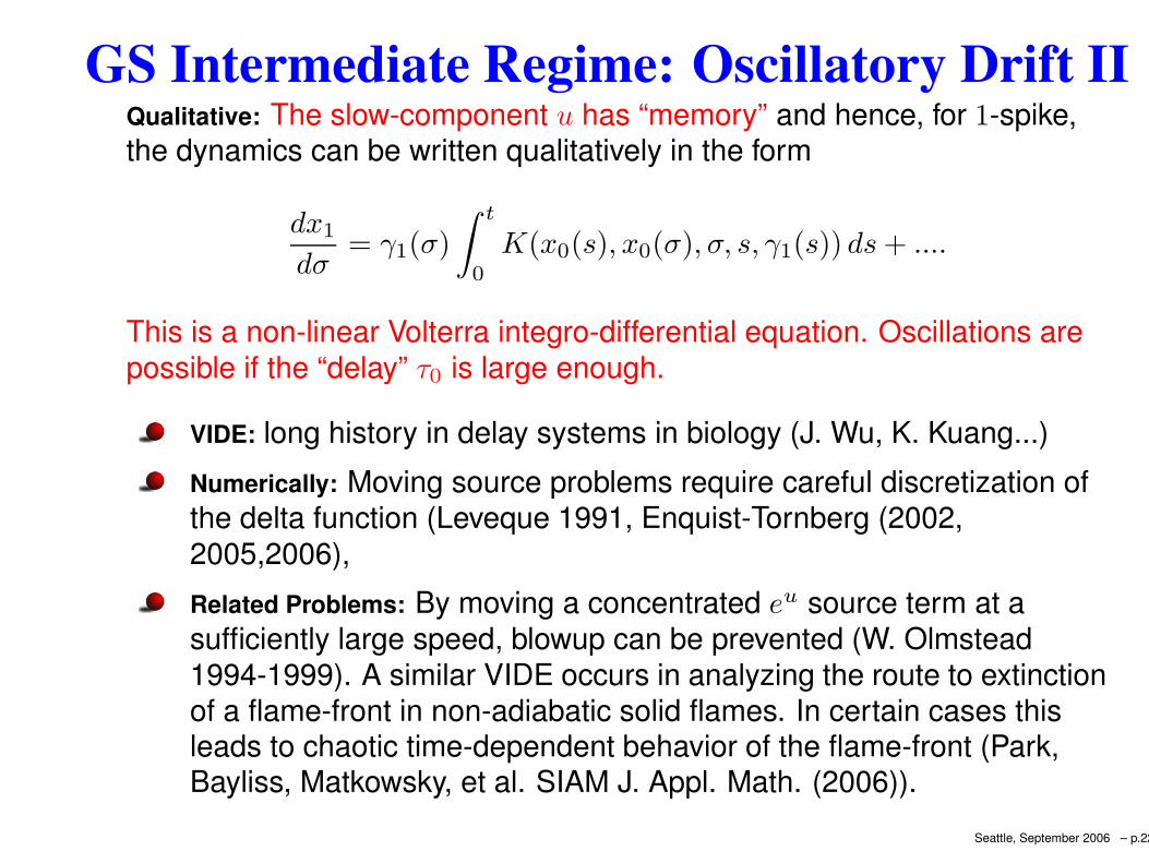
GS Intermediate Regime: Oscillatory Drift IIQualitative: The slow-component u has “memory” and hence, for 1-spike,the dynamics can be written qualitatively in the form

dx1

dσ= γ1(σ)

∫ t

0

K(x0(s), x0(σ), σ, s, γ1(s)) ds + ....

This is a non-linear Volterra integro-differential equation. Oscillations arepossible if the “delay” τ0 is large enough.

VIDE: long history in delay systems in biology (J. Wu, K. Kuang...)Numerically: Moving source problems require careful discretization ofthe delta function (Leveque 1991, Enquist-Tornberg (2002,2005,2006),Related Problems: By moving a concentrated eu source term at asufficiently large speed, blowup can be prevented (W. Olmstead1994-1999). A similar VIDE occurs in analyzing the route to extinctionof a flame-front in non-adiabatic solid flames. In certain cases thisleads to chaotic time-dependent behavior of the flame-front (Park,Bayliss, Matkowsky, et al. SIAM J. Appl. Math. (2006)).


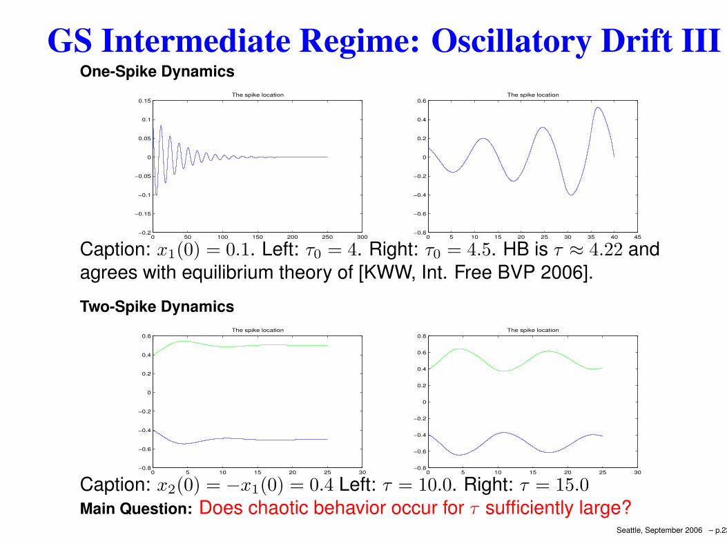
GS Intermediate Regime: Oscillatory Drift IIIOne-Spike Dynamics

0 50 100 150 200 250 300−0.2

−0.15

−0.1

−0.05

0

0.05

0.1

0.15The spike location

0 5 10 15 20 25 30 35 40 45−0.8

−0.6

−0.4

−0.2

0

0.2

0.4


Caption: x1(0) = 0.1. Left: τ0 = 4. Right: τ0 = 4.5. HB is τ ≈ 4.22 andagrees with equilibrium theory of [KWW, Int. Free BVP 2006].Two-Spike Dynamics

0 5 10 15 20 25 30−0.8

−0.6

−0.4

−0.2

0

0.2

0.4


0 5 10 15 20 25 30−0.8

−0.6

−0.4

−0.2

0

0.2

0.4

0.6


Caption: x2(0) = −x1(0) = 0.4 Left: τ = 10.0. Right: τ = 15.0Main Question: Does chaotic behavior occur for τ sufficiently large?


GS High-Feed Regime: Equilibria IOn |x| < 1 with A = O(1), or A = O(ε−1/2), we have

vt = ε2vxx − v + Auv2 , τut = Duxx + (1 − u) − uv2 .

Principal Result:[KWW, 2004]: The inner solution for a k-spike equilibria

v ∼√

D

ε

k∑

j=1

V[

ε−1(x − xj)]

, u ∼ ε

A√

D

k∑

j=1

U[

ε−1(x − xj)]

.

Here U(y) and V (y) satisfy the core problem on 0 < y < ∞:

V′′ − V + V 2U = 0 , U

′′

= UV 2 ,

V′

(0) = U′

(0) = 0 ; V → 0 , U ∼ By , as y → ∞ .

Core problem identified by Doelman et. al (1998), Muratov-Osipov (2000).Matching of core problem to outer solution for u involving Green’s functions

(KWW, 2004). Detailed properties of bifurcation diagram (DKP, 2006).Seattle, September 2006 – p.24

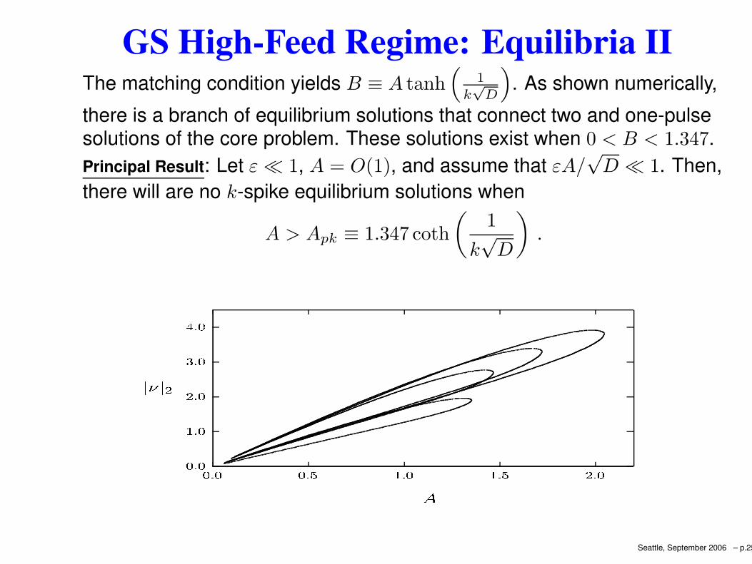
GS High-Feed Regime: Equilibria IIThe matching condition yields B ≡ A tanh

(

1

k√

D

)

. As shown numerically,there is a branch of equilibrium solutions that connect two and one-pulsesolutions of the core problem. These solutions exist when 0 < B < 1.347.Principal Result: Let ε 1, A = O(1), and assume that εA/

√D 1. Then,

there will are no k-spike equilibrium solutions when

A > Apk ≡ 1.347 coth

(

1

k√

D

)

.


GS High-Feed Regime: Drift Instability IOscillatory profile instabilities occur when τ = O(ε−2). Oscillatory driftinstabilities occur when τ = O(ε−1).Principal Result:[KWW, 2004]: Let ε 1 and εA/

√D 1. Then, the k

small eigenvalues λj for j = 1, . . . , k associated with drift instabilities ofthe k-spike equilibrium solution satisfy

λ ∼ εαA√D

[√1 + τλ tanh

(

θ0

k

)

zj − 1

]

, θλ ≡ θ0

√1 + τλ ,

zj = coth

(

2θλ

k

)

+ csch(

2θλ

k

)

cos

(

πj

k

)

, θ0 = D−1/2 .

Here the constant α > 0 is given by α ≡ −Ψ†2(∞)/

∫∞0

Ψ†1Vy dy, where

L†Ψ† ≡(

Ψ†1yy

Ψ†2yy

)

+

(

−1 + 2UV −2UV

V 2 −V 2

)(

Ψ†1

Ψ†2

)

= 0 ,

and Ψ1 → 0 and Ψ2y → 0 as |y| → ∞.


GS High-Feed Regime: Drift Instability IIIn the inner region near the jth spike, the spatial form of such aninstability for δ 1 is

v(x, t) ∼√

D

ε

(

V [ε−1(x − xj)] + δcjVy[ε−1(x − xj)]eλt)

.

where ctk =

(

1,−1, . . . , (−1)k+1)

. The other k − 1 possible modes ofinstabilty satisfy

cl,j = sin

(

πj

k(l − 1/2)

)

, j = 1, . . . , k − 1 , l = 1, . . . , k .

Our analysis shows that the primary branch is stable when τ O(ε−1).Instabilities can only occur when τ = O(ε−1) through oscillatory driftinstabilities (Hopf bifurcations) in the spike locations.


GS High-Feed Regime: Drift Instability IIIPrincipal Result: [KWW, 2004]: Let ε 1, τ = O(ε−1), and εA/

√D 1.

Then, along the primary branch of the equilibrium core problem, thek-spike equilibrium solution is stable when 0 < τ < τTW , and is unstablewhen τ > τTW . The stability is lost due to a Hopf bifurcation in the spikelocations when τ = τTW , where

τTW ∼(√

D

εαA

)

τdh , τdh ≡ minj=1,...,k

(τdj) .

Here τdj for j = 1, . . . , k is defined by

τdj ≡ ξIj

Im(Gj(iξIj)), j = 1, . . . , k ; Fj(iξIj) = 0 ,

Fj(ξ) ≡ξ

τd− Gj(ξ) , Gj(ξ) ≡

√

1 + ξ tanh

(

θ0

k

)

zj(ξ) − 1 ,

zj(ξ) ≡ coth

(

2θ0

√1 + ξ

k

)

+ csch(

2θ0

√1 + ξ

k

)

cos

(

πj

k

)

− 1 .


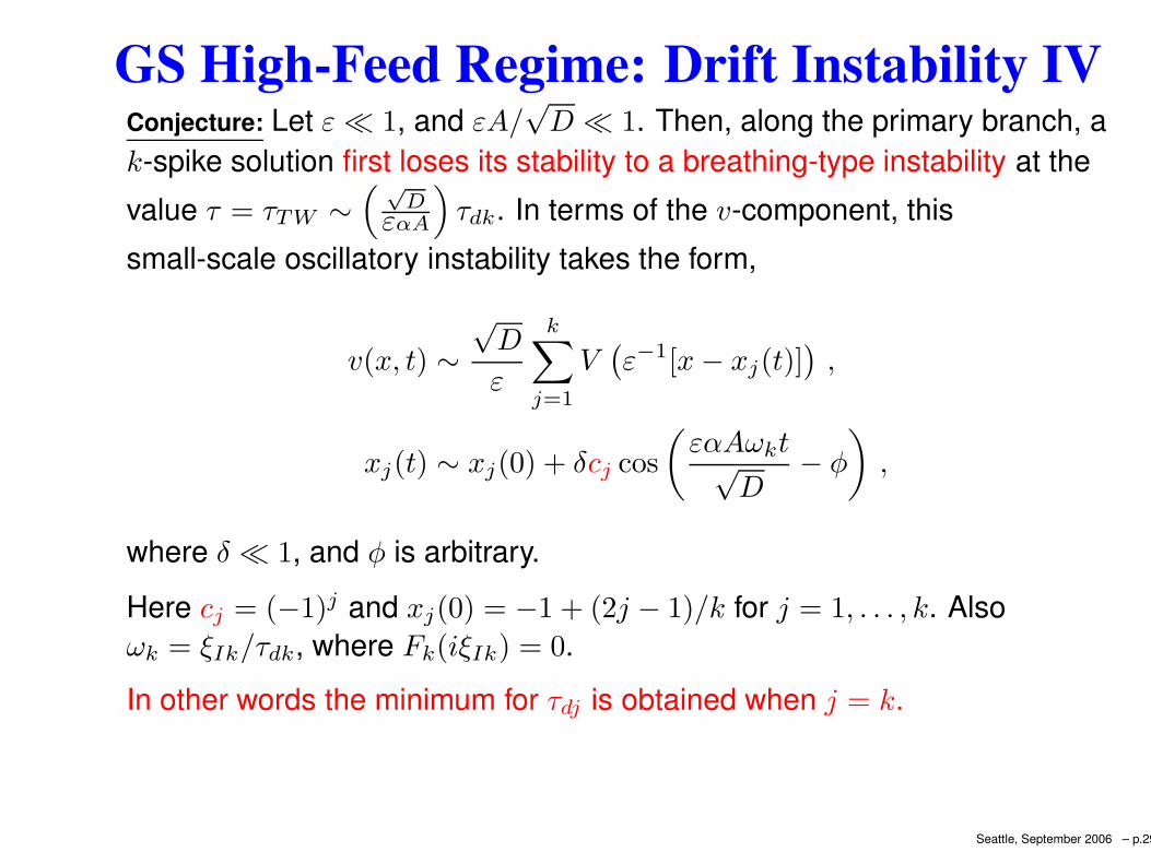
GS High-Feed Regime: Drift Instability IVConjecture: Let ε 1, and εA/

√D 1. Then, along the primary branch, a

k-spike solution first loses its stability to a breathing-type instability at thevalue τ = τTW ∼

( √D

εαA

)

τdk. In terms of the v-component, thissmall-scale oscillatory instability takes the form,

v(x, t) ∼√

D

ε

k∑

j=1

V(

ε−1[x − xj(t)])

,

xj(t) ∼ xj(0) + δcj cos

(

εαAωkt√D

− φ

)

,

where δ 1, and φ is arbitrary.Here cj = (−1)j and xj(0) = −1 + (2j − 1)/k for j = 1, . . . , k. Alsoωk = ξIk/τdk, where Fk(iξIk) = 0.In other words the minimum for τdj is obtained when j = k.


GS High-Feed Regime: Drift Instability V

"

¡¢

£¤¥ £

¥ £ £¦¥ £

§ £ £ £¨ §"© £ ¨ £© ¥ £© £ £© ¥ § © £

ª

«¬

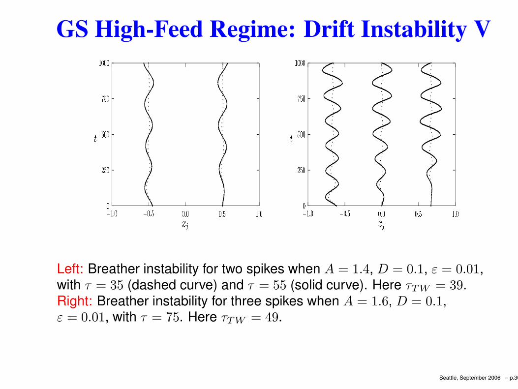
Left: Breather instability for two spikes when A = 1.4, D = 0.1, ε = 0.01,with τ = 35 (dashed curve) and τ = 55 (solid curve). Here τTW = 39.Right: Breather instability for three spikes when A = 1.6, D = 0.1,ε = 0.01, with τ = 75. Here τTW = 49.


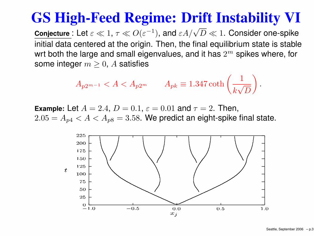
GS High-Feed Regime: Drift Instability VIConjecture : Let ε 1, τ O(ε−1), and εA/

√D 1. Consider one-spike

initial data centered at the origin. Then, the final equilibrium state is stablewrt both the large and small eigenvalues, and it has 2m spikes where, forsome integer m ≥ 0, A satisfies

Ap2m−1 < A < Ap2m Apk ≡ 1.347 coth

(

1

k√

D

)

.

Example: Let A = 2.4, D = 0.1, ε = 0.01 and τ = 2. Then,2.05 = Ap4 < A < Ap8 = 3.58. We predict an eight-spike final state.

®¯

¯ °¯

± ± ®¯

± ¯ ± °¯

® ® ®¯

² ±³ ² ³ ¯ ³ ³ ¯ ±³

´

µ¶


GS High-Feed: Large Drift Instability I

·¸¹ ·

¹ · ·º¹ ·

» · · ·¼ »"½ · ¼ ·½ ¹ ·½ · ·½ ¹ »½ ·

¾

¿À

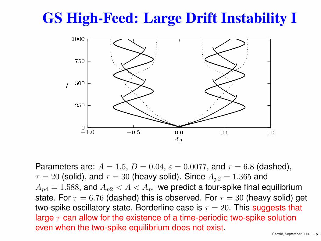
Parameters are: A = 1.5, D = 0.04, ε = 0.0077, and τ = 6.8 (dashed),τ = 20 (solid), and τ = 30 (heavy solid). Since Ap2 = 1.365 andAp4 = 1.588, and Ap2 < A < Ap4 we predict a four-spike final equilibriumstate. For τ = 6.76 (dashed) this is observed. For τ = 30 (heavy solid) gettwo-spike oscillatory state. Borderline case is τ = 20. This suggests thatlarge τ can allow for the existence of a time-periodic two-spike solutioneven when the two-spike equilibrium does not exist.


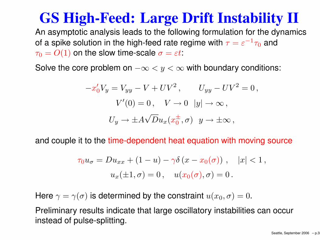
GS High-Feed: Large Drift Instability IIAn asymptotic analysis leads to the following formulation for the dynamicsof a spike solution in the high-feed rate regime with τ = ε−1τ0 andτ0 = O(1) on the slow time-scale σ = εt:Solve the core problem on −∞ < y < ∞ with boundary conditions:

−x′0Vy = Vyy − V + UV 2 , Uyy − UV 2 = 0 ,

V ′(0) = 0 , V → 0 |y| → ∞ ,

Uy → ±A√

Dux(x±0 , σ) y → ±∞ ,

and couple it to the time-dependent heat equation with moving source

τ0uσ = Duxx + (1 − u) − γδ (x − x0(σ)) , |x| < 1 ,

ux(±1, σ) = 0 , u(x0(σ), σ) = 0 .

Here γ = γ(σ) is determined by the constraint u(x0, σ) = 0.Preliminary results indicate that large oscillatory instabilities can occurinstead of pulse-splitting.


ReferencesD. Iron, M. J. Ward, J. Wei, The Stability of Spike Solutions to theOne-Dimensional Gierer-Meinhardt Model, Physica D. Vol. 150,(2001) pp. 25-62.D. Iron, M. J. Ward, The Dynamics of Multi-Spike Solutions for theOne-Dimensional Gierer-Meinhardt Model, SIAM J. Appl. Math., Vol.62, No. 6, (2002), pp. 1924-1951.W. Sun, M. J. Ward, R. Russell, The Slow Dynamics of Two-SpikeSolutions for the Gray-Scott and Gierer-Meinhardt Systems:Competition and Oscillatory Instabilities, SIADS, Dec. (2005).T. Kolokolnikov, M. J. Ward, Reduced Wave Green’s Functions andtheir Effect on the Dynamics of a Spike for the Gierer-MeinhardtModel, EJAM, Vol. 14, No. 5, (2003), pp. 513-545.W. Chen, M. J. Ward, Oscillatory Drift and Profile Instabilities for theGray-Scott Model on a Finite Interval, in preparation.


Oscillatory and Competition Instabilities: Dynamics of ...ward/papers/nonwaves.pdf · Dynamic...

Documents

Transcript of Oscillatory and Competition Instabilities: Dynamics of ...ward/papers/nonwaves.pdf · Dynamic...