Absolute and Convective Instabilities in Parallel Flows ...onaraigh/simsci/lecture_notes.pdf ·...

Absolute and Convective Instabilities in ParallelFlows

Lecture 1

Dr Lennon O Naraigh

1 Overview and Workplan

The idea of these four lectures is to study the asymptotic (t → ∞) properties of thefollowing equation from the linear theory of parallel flow instability:

∂

∂t∇2ϕ+ U0(z)∇2∂ϕ

∂x− U ′′

0 (z)∂ϕ

∂x=

1

Re∇4ϕ, (1a)

with boundary conditions

ϕ = ϕz = 0, at z = 0, 1, (1b)

andlim

|x|→∞ϕ = lim

|x|→∞ϕx = 0, (1c)

subject to an initial impulsive disturbance

ϕ(x, z, t = 0) = δ(x− x0)δ(z − z0). (1d)

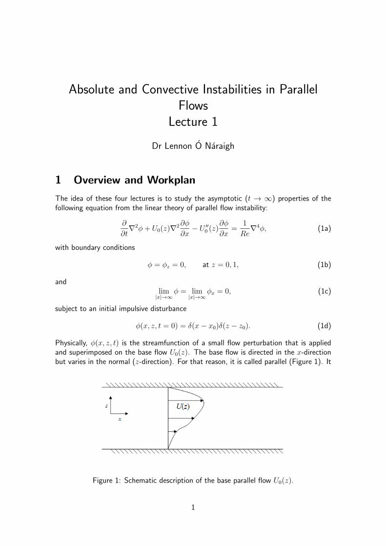
Physically, ϕ(x, z, t) is the streamfunction of a small flow perturbation that is appliedand superimposed on the base flow U0(z). The base flow is directed in the x-directionbut varies in the normal (z-direction). For that reason, it is called parallel (Figure 1). It

Figure 1: Schematic description of the base parallel flow U0(z).

1

Absolute and Convective Instabilities in Parallel Flows Lecture 1

is of interest to know whether this perturbation will grow over time or decay. The flowis called convectively unstable if

limt→∞

|ϕ(x, z, t)| = ∞,

for some x. The flow is called absolutely unstable if

limt→∞

|ϕ(x0, z0, t)| = ∞.

That is, convectively unstable disturbances grow as they are convected downstream bythe base flow U0(z), while absolutely unstable disturbances grow at the disturbancesource.

The problem is first of all approached by studying the theory of Laplace transforms.In the first two lectures, this will be our exclusive focus.

2 Laplace transforms

In this section, let

F : [0,∞) → C,t 7→ F (t) (2)

be a complex-valued function of a real variable.

Definition 2.1 Let The function F (t) is at most exponentially diverging if thereexist real numbers (λ0,M > 0) such that

|e−λ0tF (t)| ≤ M, as t → ∞;

we call λ0 the divergence parameter.

Definition 2.2 Let F (t) be at most exponentially diverging, with divergence parameterλ0. Laplace-transform of F (t) is defined as follows:

Fλ ≡ L(F ) :=

∫ ∞

0

e−λtF (t)dt, ℜ(λ) > λ0.

Theorem 2.1 The Laplace transform is linear, in the sense that

L(αF (t) + βG(t)) = αL(F ) + βL(G),

where α and β are complex conostants and the functions F and G are functions oftype (2) whose Laplace transforms exist.

2


Examples

1. Let F (t) = ekt, with k > 0 real. We have

Fλ =

∫ ∞

0

e(k−λ)tdt,

= limL→∞

[1

k − λ

(e(k−λ)L − 1

)]. (3)

Obviously, we need ℜ(λ) > k for this integral to exist, hence

Fλ =1

λ− k, ℜ(λ) > k.

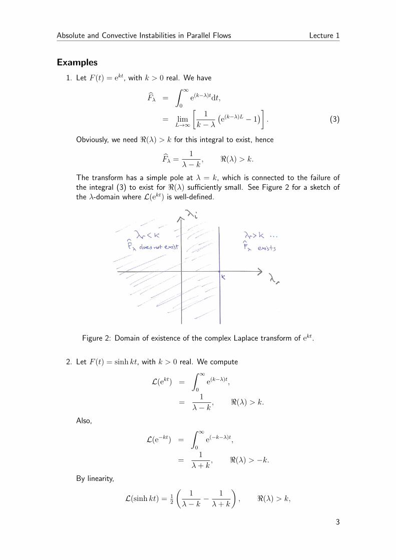
The transform has a simple pole at λ = k, which is connected to the failure ofthe integral (3) to exist for ℜ(λ) sufficiently small. See Figure 2 for a sketch ofthe λ-domain where L(ekt) is well-defined.

Figure 2: Domain of existence of the complex Laplace transform of ekt.

2. Let F (t) = sinh kt, with k > 0 real. We compute

L(ekt) =

∫ ∞

0

e(k−λ)t,

=1

λ− k, ℜ(λ) > k.

Also,

L(e−kt) =

∫ ∞

0

e(−k−λ)t,

=1

λ+ k, ℜ(λ) > −k.

By linearity,

L(sinh kt) = 12

(1

λ− k− 1

λ+ k

), ℜ(λ) > k,

3


where the first inequality trumps the second one. Finally,

L(sinh kt) = k

λ2 − k2, ℜ(λ) > k.

3. Let F (t) = δ(t− t0), with t0 > 0. We have

Fλ =

∫ ∞

0

eλtδ(t− t0) = eλt0 .

We take t0 ↓ 0 and defineL(δ(t)) = 1.

3 Inverting Laplace transforms

Let

F : [0,∞) → C,t 7→ F (t)

be a complex-valued function of a real variable, and moreover, let F (t) be at worstexponentially diverging, with exponential parameter λ0. We re-write F (t) as

F (t) = eγtG(t),

where limt→∞ G(t) = 0. Such a G-function exists; we take

G(t) = F (t)e−(λ0+ϵ)t,

for ϵ arbitrary and positive (hence, γ = λ0 + ϵ). We have

|G(t)| = |F (t)|e−λ0t−ϵt,

≤ Meλ0te−λ0t−ϵt, as t → ∞,

≤ Me−ϵt,

→ 0, as t → ∞.

Also, define G(t) = 0 for t < 0. It follows that G is L2 square integrable. Subject to theusual further conditions on G (i.e. piecewise differentiable for t ∈ R), G can be writtenin Fourier transform notation:

G(t) =

∫ ∞

−∞

dω

2πeiωtGω,

=

∫ ∞

−∞

dω

2πeiωt

[∫ ∞

−∞ds e−iωsG(s)

]Multiply across by eγt:

eγtG(t) =eγt

2π

∫ ∞

−∞dω eiωt

[∫ ∞

−∞ds e−iωsG(s)

],

F (t) =eγt

2π

∫ ∞

−∞dω eiωt

[∫ ∞

0

ds e−iωsF (s)e−γs

],

=eγt

2π

∫ ∞

−∞dω eiωt

[∫ ∞

0

ds e−λsF (s)

]︸︷︷︸

=Fλ

.

4


Let λ = γ + iω, hence ω = (λ− γ)/i.

F (t) =eγt

2π

∫ ∞

−∞

(dω eiωt

)ω=λ−γ

i

Fλ.

Effecting the change of variables, this is

F (t) =1

2π

∫ ∞

−∞

(dω e(γ+iω)t

)ω=λ−γ

i

Fλ,

=1

2πi

∫ γ+i∞

γ−i∞dλ eλtFλ.

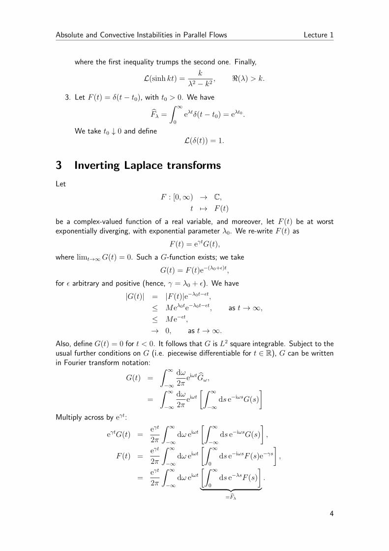
The contourB = {z ∈ C|z = γ + iy, y ∈ R}

is called the Bromwich contour. It is sketched in Figure 3.

Figure 3: Definition sketch – the Bromwich contour

Suppose now thatlimλ→∞

|eλtFλ| = 0, t > 0

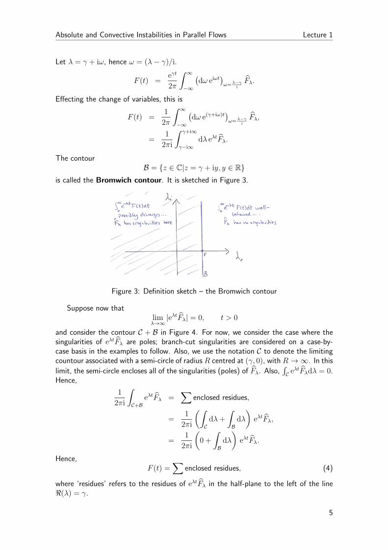
and consider the contour C + B in Figure 4. For now, we consider the case where thesingularities of eλtFλ are poles; branch-cut singularities are considered on a case-by-case basis in the examples to follow. Also, we use the notation C to denote the limitingcountour associated with a semi-circle of radius R centred at (γ, 0), with R → ∞. In this

limit, the semi-circle encloses all of the singularities (poles) of Fλ. Also,∫C e

λtFλdλ = 0.Hence,

1

2πi

∫C+B

eλtFλ =∑

enclosed residues,

=1

2πi

(∫Cdλ+

∫Bdλ

)eλtFλ,

=1

2πi

(0 +

∫Bdλ

)eλtFλ.

Hence,F (t) =

∑enclosed residues, (4)

where ‘residues’ refers to the residues of eλtFλ in the half-plane to the left of the lineℜ(λ) = γ.

5


Figure 4: Integration along the Bromwich contour using the Residue Theorem

Example

Let f(λ) = k/(λ2 − k2), with k > 0 real. If f(λ) is a Laplace transform, compute thegenerating function of the transofrm.

We compute

F (t) =1

2πi

∫B

keλt

λ2 − k2dλ,

where B is the Bromiwch contours: it is a straight line parallel to the imaginary axis tothe right of the singularities of the integrand

keλt

λ2 − k2. (5)

Since the singularites of Equation (5) are λ = ±k, the Bromwich contour is

B = {z ∈ C|z = (k + ϵ) + iy, y ∈ R, ϵ > 0}.

Using the residue theorem, we have

F (t) = Res

(keλt

λ2 − k2, k

)+Res

(keλt

λ2 − k2,−k

)= lim

λ→k

[(λ− k)

keλt

λ2 − k2

]+ lim

λ→−k

[(λ+ k)

keλt

λ2 − k2

]= 1

2

(ekt − e−kt

)= sinh(kt),

in agreement with Example 2 in Section 2.

6


4 Laplace transforms – properties

Throughout this section, let (F (t), Fλ) be a valid Laplace-transform pair:

Fλ =

∫ ∞

0

F (t)e−λtdt, F (t) =1

2πi

∫BFλe

λt,

where B is the Bromwich contour.

Theorem 4.1 (Substitution) Let a ∈ C, and let f(λ) := Fλ denote the Laplacetranform of the functioni F . Then

f(λ− a) = L(eatF (t)

).

Proof: By direct calculation we have

f(λ− a) = Fλ−a,

=

∫ ∞

0

e−(λ−a)tF (t)dt,

=

∫ ∞

0

e−λt[eatF (t)

]dt,

= L(eatF (t)

).

Theorem 4.2 (Translation) Let a be a real positive number and let f(λ) := Fλ. Then

e−bλf(λ) =

∫ ∞

0

e−λtF (t− b)H(t− b)dt,

where H(·) is the unit step function,

H(x) =

{1, x > 0,

0, x < 0.

Proof: We have

e−bλf(λ) =

∫ ∞

0

e−bλe−λtF (t) dt,

=

∫ ∞

0

e−(b+t)λF (t) dt.

Let τ = b+ t, with τlw = b and τup = ∞. Hence,

e−bλf(λ) =

∫ ∞

b

e−λτF (τ − b) dτ.

However, consider

F (τ − b)H(τ − b) =

{F (τ − b), τ > b

0, τ < b.

7


Hence,

e−bλf(λ) = 0×∫ b

0

e−λτF (τ − b) dτ + 1×∫ ∞

b

e−λτF (τ − b) dτ

=

∫ ∞

0

e−λτF (τ − b)H(τ − b) dτ.

Theorem 4.3 (Differentiation in real space) F (t) be a C1 function of t, with F

and its derivative at worst exponentially diverging. Then (dF/dt)λ exists and(dF

dt

)λ

=

∫ ∞

0

λe−λtF (t)dt− F (0).

Proof: By assumption, dF/dt is at worst exponentially diverging, and its Laplacetransform exists, at least for appropriate λ-values. Also by definition,(

dF

dt

)λ

=

∫ ∞

0

e−λtdF

dtdt,

=

∫ ∞

0

[d

dt

(e−λtF

)+ λe−λtF

]dt,

= limL→∞

e−λLF (L)− F (0) +

∫ ∞

0

λe−λtF (t)dt.

For ℜ(λ) sufficiently large and positive, the limiting boundary term vanishes, and(dF

dt

)λ

∫ ∞

0

λe−λtF (t)dt− F (0),

as required.

Theorem 4.4 (Differentiation in transform space) F (t) be piecewise differentiable

with respect to t. Then f(λ) := Fλ is differentiable with respect to λ and, moreover,

f ′(λ) = L (−tF (t)) .

Proof: For suitable λ, the integral

f(λ) =

∫ ∞

0

e−λtF (t)dt

is well-defined and is uniformly convergent and may be differentiated under the integralsign with respect to λ. We compute:

f ′(λ) =d

dλ

∫ ∞

0

e−λtF (t)dt,

=

∫ ∞

0

[∂

∂λe−λt

]F (t)dλ,

=

∫ ∞

0

e−λt [−tF (t)] dt,

= L (−tF (t)) .

8


Definition 4.1 (Convolution) Let F (t) and G(t) be at-worst exponentially diverging.The convolution of F and G is defined as

(F ∗G)(t) =

∫ t

0

F1(t− τ)F2(τ)dτ.

Theorem 4.5 (by Faltung) Let F (t) and G(t) be at-worst exponentially diverging,

with Laplace transforms Fλ and Gλ respectively. Then

FλGλ = L [(F ∗G)(t)]

Proof: Given in Lecture 2.

9


Lecture 2

Dr Lennon O Naraigh

1 Laplace transforms, examples

In this section, let

F : [0,∞) → C,t 7→ F (t) (1)

be a complex-valued function of a real variable, such that

|e−λ0tF (t)| ≤ M, as t → ∞;

The Laplace tranform of F (t) is defined as follows:

Fλ ≡ L(F ) :=

∫ ∞

0

e−λtF (t)dt, ℜ(λ) > λ0.

Given that f(λ) = λ−1/2 is the Laplace transform of a function, find the generatingfunction.

We must ascribe an unambiguous meaning to f(z) = z1/2. We have two possibilities:

f(z) = |z|1/2{cos(θ/2) + i sin(θ/2),

cos(π + θ/2) + i sin(π + θ/2),

where θ = arg(z). The standard choice is to take f(z) = |z|1/2 [cos(θ/2) + i sin(θ/2)].This introduces a discontinuity in f(z) across the half-line x > 0, since f(x, 0+ϵ) =

√x,

while f(x, 2π − ϵ) =√x cos(π), and

f(x, 0 + ϵ)− f(x, 2π − ϵ) = 2√x, x > 0.

However, we are interested in a situation where the discontinuity should occur acrossthe half-line x < 0. We therefore unambiguously define

f(z) = |z|1/2{cos(θ/2) + i sin(θ/2), 0 ≤ θ < π,

cos(π + θ/2) + i sin(π + θ/2), π < θ ≤ 2π:= |z|1/2Θ(θ).

1


0 2 4 60

0.2

0.4

0.6

0.8

1

θ

Θr

(a)

0 2 4 6−1

−0.5

0

0.5

1

θ

Θi

(b)

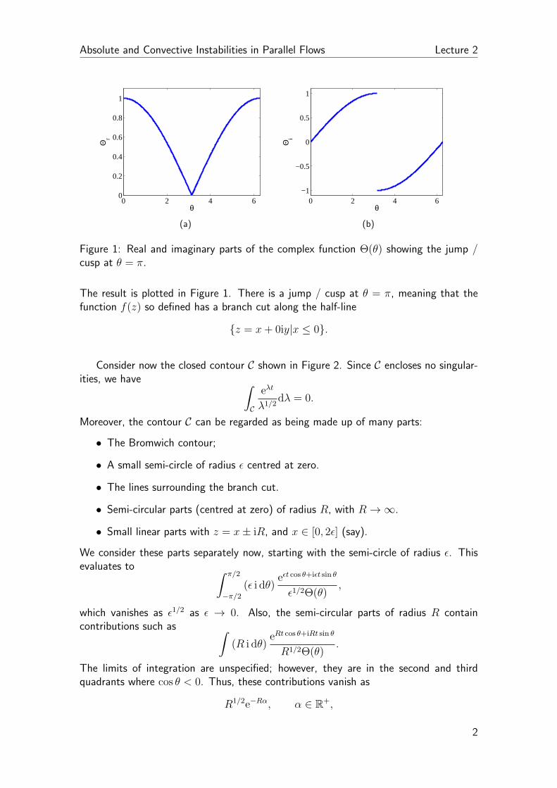
Figure 1: Real and imaginary parts of the complex function Θ(θ) showing the jump /cusp at θ = π.

The result is plotted in Figure 1. There is a jump / cusp at θ = π, meaning that thefunction f(z) so defined has a branch cut along the half-line

{z = x+ 0iy|x ≤ 0}.

Consider now the closed contour C shown in Figure 2. Since C encloses no singular-ities, we have ∫

C

eλt

λ1/2dλ = 0.

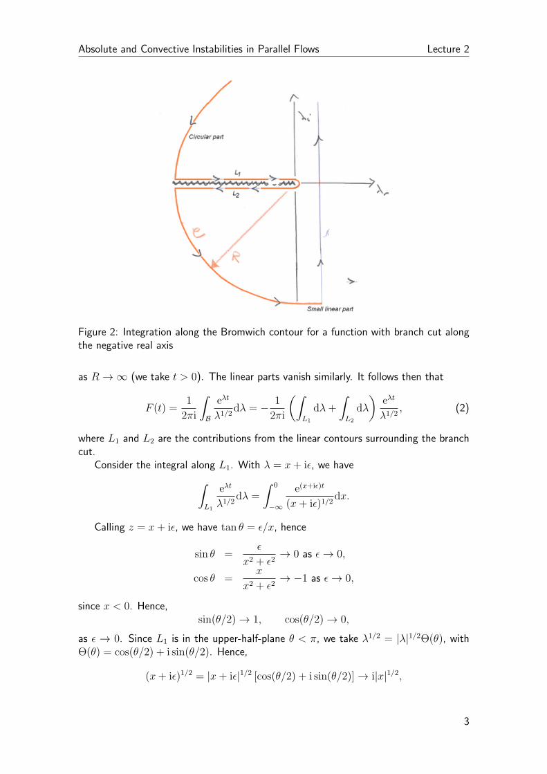
Moreover, the contour C can be regarded as being made up of many parts:

• The Bromwich contour;

• A small semi-circle of radius ϵ centred at zero.

• The lines surrounding the branch cut.

• Semi-circular parts (centred at zero) of radius R, with R → ∞.

• Small linear parts with z = x± iR, and x ∈ [0, 2ϵ] (say).

We consider these parts separately now, starting with the semi-circle of radius ϵ. Thisevaluates to ∫ π/2

−π/2

(ϵ i dθ)eϵt cos θ+iϵt sin θ

ϵ1/2Θ(θ),

which vanishes as ϵ1/2 as ϵ → 0. Also, the semi-circular parts of radius R containcontributions such as ∫

(R i dθ)eRt cos θ+iRt sin θ

R1/2Θ(θ).

The limits of integration are unspecified; however, they are in the second and thirdquadrants where cos θ < 0. Thus, these contributions vanish as

R1/2e−Rα, α ∈ R+,

2


Figure 2: Integration along the Bromwich contour for a function with branch cut alongthe negative real axis

as R → ∞ (we take t > 0). The linear parts vanish similarly. It follows then that

F (t) =1

2πi

∫B

eλt

λ1/2dλ = − 1

2πi

(∫L1

dλ+

∫L2

dλ

)eλt

λ1/2, (2)

where L1 and L2 are the contributions from the linear contours surrounding the branchcut.

Consider the integral along L1. With λ = x+ iϵ, we have∫L1

eλt

λ1/2dλ =

∫ 0

−∞

e(x+iϵ)t

(x+ iϵ)1/2dx.

Calling z = x+ iϵ, we have tan θ = ϵ/x, hence

sin θ =ϵ

x2 + ϵ2→ 0 as ϵ → 0,

cos θ =x

x2 + ϵ2→ −1 as ϵ → 0,

since x < 0. Hence,sin(θ/2) → 1, cos(θ/2) → 0,

as ϵ → 0. Since L1 is in the upper-half-plane θ < π, we take λ1/2 = |λ|1/2Θ(θ), withΘ(θ) = cos(θ/2) + i sin(θ/2). Hence,

(x+ iϵ)1/2 = |x+ iϵ|1/2 [cos(θ/2) + i sin(θ/2)] → i|x|1/2,

3


as ϵ ↓ 0. Thus, we have the following string of relations:∫L1

eλt

λ1/2dλ =

∫ 0

−∞

e(x+iϵ)t

(x+ iϵ)1/2dx,

ϵ↓0=

∫ 0

−∞

ext

i|x|1/2dx,

=

∫ 0

−∞

ext

i(−x)1/2dx,

y=−x=

1

i

∫ ∞

0

e−yt

y1/2dy,

X=(ty)1/2

=2

i

∫ ∞

0

e−X2

dX,

=2

i

(12

√π/t

),

=1

i

√π/t.

We make similar arguments for the second linear contouor. We write λ = x − iϵ,such that ∫

L2

eλt

λ1/2dλ = −

∫ 0

−∞

e(x−iϵ)t

(x− iϵ)1/2dx.

Calling z = x− iϵ, we have tan θ = ϵ/x, hence

sin θ =ϵ√

x2 + ϵ2→ 0 as ϵ → 0,

cos θ =x√

x2 + ϵ2→ −1 as ϵ → 0,

since x < 0. Since L2 is in the lower-half-plane θ < π, we take Θ(θ) = cos(π + θ/2) +i sin(π + θ/2), hence

sin(π + θ/2) → −1, cos(π + θ/2) → 0,

as ϵ → 0. Again taking Θ(θ) = cos(π + θ/2) + i sin(π + θ/2), we have

(x− iϵ)1/2 = |x− iϵ|1/2 [cos(π + θ/2) + i sin(π + θ/2)] → −i|x|1/2,as ϵ ↓ 0. Then, as before, we consider the following string of relations:∫

L2

eλt

λ1/2dλ = −

∫ 0

−∞

e(x−iϵ)t

(x− iϵ)1/2dx,

ϵ↓0= −

∫ 0

−∞

ext

−i|x|1/2dx,

= +

∫ 0

−∞

ext

|x|1/2dx,

=1

i

√π/t.

From Equation (2), we have

F (t) = − 1

2πi

(∫L1

dλ+

∫L2

dλ

)eλt

λ1/2= − 1

2πi

(2

i

√π/t

)=

1√πt

.

4


2 Laplace transforms – properties

Definition 2.1 (Convolution) Let F (t) and G(t) be at-worst exponentially diverging.The convolution of F and G is defined as

(F ∗G)(t) =

∫ t

0

F1(t− τ)F2(τ)dτ.

Theorem 2.1 (by Faltung) Let F (t) and G(t) be at-worst exponentially diverging,

with Laplace transforms Fλ and Gλ respectively. Then

FλGλ = L [(F ∗G)(t)]

Proof: By direct computation, we have

FλGλ =

∫ ∞

0

e−λtF (t) dt

∫ ∞

0

e−λsG(s) ds.

We first of all re-write the integral as follows:

FλGλ = limL→∞

∫ L

0

e−λtF (t)dt

∫ L

0

e−λsG(s) ds.

The trick is to re-write this further as

FλGλ = limL→∞

∫ L

0

e−λtF (t) dt

∫ L−t

0

e−λsG(s) ds.

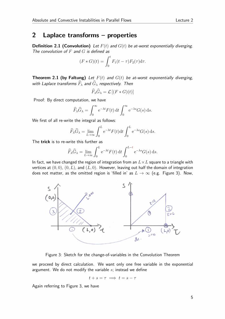
In fact, we have changed the region of integration from an L×L square to a triangle withvertices at (0, 0), (0, L), and (L, 0). However, leaving out half the domain of integrationdoes not matter, as the omitted region is ‘filled in’ as L → ∞ (e.g. Figure 3). Now,

Figure 3: Sketch for the change-of-variables in the Convolution Theorem

we proceed by direct calculation. We want only one free variable in the exponentialargument. We do not modify the variable s; instead we define

t+ s = τ =⇒ t = s− τ

Again referring to Figure 3, we have

5


• Line Segment 1 (s = 0) is mapped to s = 0;

• Line Segment 2 (s = L− t) implies that τ = t + (L− t) = L (constant); henceline-segment 2 is mapped to a vertical line segment passing through τ = L.

• The condition on Line Segment 3 (t = 0) implies s = τ , hence line segment 3 ismapped to the straight line of slope 45o passing through the origin.

Also, consider the transformation, expressed correctly here as

τ = t+ s,

s′ = s,

with inverse

t = τ − s′,

s = s′.

We have

dt ds =

∣∣∣∣ ∂t∂τ

∂t∂s′

∂s∂τ

∂s′

∂s

∣∣∣∣︸︷︷︸=J

dτ ds′.

J =

∣∣∣∣ 1 −10 1

∣∣∣∣ = 1,

hencedt ds = dτ ds′.

Putting it all together, we have

FλGλ = limL→∞

∫ L

0

e−λtF (t) dt

∫ L−t

0

e−λsG(s) ds,

= limL→∞

∫ L

0

dt

∫ L−t

0

ds e−λtF (t)e−λsG(s),

= limL→∞

∫ L

0

dτ

∫ τ

0

ds F (τ − s)e−λ(τ−s)G(s)e−λs,

= limL→∞

∫ L

0

dτ e−λτ

∫ τ

0

ds F (τ − s)G(s),

=

∫ ∞

0

dτ e−λτ

[∫ τ

0

ds F (τ − s)G(s)

],

=

∫ ∞

0

dτ e−λτ (F ∗G)(τ),

= L[(F ∗G)(τ)].

6


Example

Compute the inverse transform of

f(λ) =1− e−aλ

λ, a ∈ R+.

We break it up into two parts. Consider

I1 =1

2πi

∫B

eλt

λdλ.

The Bromwich contour is a straight line parallel to the imaginary axis passing throughz = 0 + iϵ, with ϵ ↓ 0. The integrand has a single simple pole at λ = 0, with

Res

(eλt

λ, 0

)= 1.

Hence,I1 = 1, t > 0.

On the other hand, if t < 0, to get a convergent integral we would have to close thecontour by forming a semi-circle on the right of the Bromwich line. However, such acontour encloses no singularities, hence

I1 = 0, t < 0.

We do the second integral by considering

I2 =1

2πi

∫B

e(t−a)λ

λdλ.

The integrand iseλr(t−a)eλi(t−a)

λ

The Bromwich contour is the same as before. For the B-contour given there are twopossibilities:

1. t− a > 0 – chose λr < 0 – close the contour on the left. Thus, a contribution tothe integral is picked up from the pole at λ = 0.

2. t − a < 0 – chose λr > 0 – close the contour on the right. Thus, there are nopole-contributions to the integral and the integal vanishes.

In other words,

I2 =

{1, if t > a,

0, if t < 1.

Finally, the answer isF (t) = H(t)−H(t− a).

7


However, from a sketch, this can be seen to be a top-hat function:

F (t) =

0, if t < 0,

1, if 0 < t < a,

0, if t > a.

There is another way of getting at the second integral I2. From the translation theorem,we have

e−aλϕλ =

∫ ∞

0

e−λtϕ(t)H(t− a)dt,

Taking ϕ(t) = H(t), with ϕλ = 1/λ, we have

e−aλ

λ=

∫ ∞

0

e−λtH(t)H(t− a)dt,

=

∫ ∞

0

e−λtH(t− a)dt.

Hence, the Laplace transform of H(t− a) is e−aλ/λ, hence

1

2πi

∫B

(e−aλ

λ

)eλtdλ = H(t− a),

as computed already, using a direect approach.

8


Tutorial 1

Dr Lennon O Naraigh

1 Bateman Equations

Solve

dN1

dt= −λ1N1,

dN2

dt= −λ2N2 + λ1N1,

dN3

dt= λ2N2,

subject to N1(0) = n1 > 0, N2(0) = n2 ≥ 0, and N3(0) = n3 ≥ 0, where (λ1, λ2, λ3)are positive constants.

2 Poles other than simple poles

Solved2x

dt2− 2

dx

dt+ x = 0,

subject to x(t = 0) = x0 and (t = 0) = v0.

1


Lecture 3

Dr Lennon O Naraigh

1 Background

We are interested in the following Cauchy problem:

∂

∂t∇2ϕ+ U0(z)∇2∂ϕ

∂x− U ′′

0 (z)∂ϕ

∂x=

1

Re∇4ϕ, (1a)


ϕ = ϕz = 0, at z = 0, 1, (1b)

andlim

|x|→∞ϕ = lim

|x|→∞ϕx = 0, (1c)


ϕ(x, z, t = 0) = δ(x− x0)δ(z − z0). (1d)

2 The solution

Equation (1a) is rewritten in Orr–Sommerfeld operator form as follows:

∂

∂tMOS[∂x, ∂z]ψ(x, z, t) = LOS[∂x, ∂z]ψ(x, z, t) + F (x, z, t), ψ(x, z, t = 0) = 0.

(2)Here, F (x, z, t) represents the momentum source; this can either be continuous-in-time,or be an initial impulse imposed on the system. In the impulsive case, S(x, z, t) =δ(t)F (x, z), with Laplace transform S(x, z, λ) = F (x, z). The solution can be writtenin terms of Fourier transforms as follows:

ψ(x, z, t) =

∫ ∞

−∞

dα

2πeiαxψα(z, t),

where the Fourier coefficients ψα(z, t) satisfy

∂

∂tMOS[iα, ∂z]ψα(z, t) = LOS[iα, ∂z]ψα(z, t) + δ(t)Fα(z, t).

1


Each Fourier component ψα(z, t) can be decomposed further via an inverse Laplacetranform:

ψα(z, t) =

∫B

dλ eλtψαλ(z),

where B is the Bromwich contour. The components ψαλ(z) of the inverse Laplacetranform in turn satisfy

λMOS(iα, z)ψαλ(z) = LOS(iα, ∂z)ψαλ(z) + Fα(z, λ), (3)

where the Laplace transform of the force function S has been taken with respect to time.This is the Orr–Sommerfeld eigenvalue problem.

The (formal) solution to Equation (3) reads

ψαλ(z) = [LOS − λMOS]−1 Fα(z, λ)

This purely formal solution is understood as follows. We write the solution of Equa-tion (3) as ψαλ(z) =

∑n anϕαn(z). Here, the ϕαn’s are the eigenfunctions of the

Orr–Sommerfeld equation at wavenumber α. Equation (3) is therefore re-written as

λ∑n

anMOSϕαn(z) =∑n

anLOSϕαn(z) + Fα(z, λ). (4)

The eigenfunctions ϕ+αm(z) of the adjoint OS problem satisfy∫

dz[ϕ+αm(z)

]∗MOSϕαn(z) = δnm.

We multiply both sides of Equation (3) by [ϕ+m(z)]

∗ and integrate with respect to z; theresult is

am =1

λ− λm

∫dz

[ϕ+αm(z)

]∗Fα(z, λ),

and

ψαλ(z) = [LOS − λMOS]−1 Fα(z, λ) =∑n

ϕαn(z)

λ− λn

∫dz

[ϕ+αn(z)

]∗Fα(z, λ) :=

∑n

ϕαn(z)Fαn(λ)

λ− λn.

Thus, the solution to the Cauchy problem (2) becomes

ψ(x, z, t) =

∫ ∞

−∞

dα

2πeiαx

∫B

dλ eλt∑n

ϕαn(z)Fαn(λ)

λ− λn, (5)

where the Bromwich contour C is a straight line parallel to the imaginary axis, to theright of all the eigenvalues {λn} of the Orr–Sommerfeld equation. A key property ofEquation (5) is the absence of any contributions from a continuous spectrum: for abounded domain z ∈ [0, 1], the spectrum of the Orr–Sommerfeld equation is entirelydiscrete.

To make progress, we make a simplifying assumption, without any loss of generality:

2


Assumption 2.1 The spectrum of the OS operator is non-degenerate:

λm = λn =⇒ m = n.

Then, each pole in the the innermost integral in Equation (5) is first-order. Using thetheory of residues, one obtains for the innermost integral

ψ(x, z, t) =∑n

∫ ∞

−∞

dα

2πeiαx+λntFαn(λn)ϕαn(z). (6)

The outermost (α-) integral can be computed in certain special cases. This is discussedin the next two sections.

3 Explicit asymptotic solutions

3.1 Monochromatic forcing

For monochromatic, impulsive forcing, F (x, z, t) = eiα0xδ(t)f(z), F (z, λ) = 2πf(z)δ(α−α0), and

Fαn(λ) = δ(α− α0)

∫dz

[ϕ+α0n

(z)]∗f(z) := δ(α− α0)fα0n.

From Equation (6),

ψ(x, z, t) =∑n

eiα0x+λn(α0)tfα0nϕα0n(z). (7)

Thus,limt→∞

ψ(x, z, t) =[fα0nmaxe

iα0x+λnmax (α0)]ϕα0nmax(z),

where nmax is that eigenvalue whose real part is maximal over the entire spectrum{λn(α0)}. Note also,

limt→∞

∥ψ∥2(t) = ∥ϕα0nmax∥2 |fα0nmax | eℜ[λnmax (α0)]t,

where ∥ · ∥2(t) is the transient L2 norm; for a function Φ(x, z, t),

∥Φ∥2(t) :=(x

dxdz|Φ(x, z, t)|2)1/2

.

Thus, as t→ ∞, the disturbance grows exponentially fast, at a rate

ℜ[λnmax(α0)].

This is called the most-dangerous mode. Obviously, if ℜ[λnmax(α0)] > 0 the systemis (convectively) unstable. The system is completely linearly stable if ℜ[λnmax(α0)] < 0.

3


3.2 Localized impulsive forcing

For localized impulsive forcing, F (x, z, t) = δ(x)δ(z−z0)δ(t), with Fα(z, λ) = δ(z−z0),and

Fαn(λ) = [ϕ+αn(z0)]

∗

Thus,

ψ(x, z, t) =∑n

∫ ∞

−∞

dα

2πeiαx+λnt[ϕ+

αn(z0)]∗ϕαn(z). (8)

This integral can be regarded as being in the form

ψ(x, z, t) =1

2π

∑n

∫ ∞

−∞dαFn(α)e

λn(α)t,

whereFn(α) = eiαx[ϕ+

αn(z0)]∗ϕαn(z)

This integral is now in a form where the saddle-point method can be applied. We needthe following additional assumptions:

Assumption 3.1

1. The phase function λn(α) has a single dominant saddle point;

2. The saddle point is not degenerate.

3. If the phase functions or the Fn(α)’s do have singularities, they are located‘far away’ from the saddle point, in the sense that they do not prevent us fromdeflecting the contour α ∈ (−∞,∞) to pass through the dominant saddlepoint.

For the dominant saddle point, we compute

1. Saddle-point location: α0, such that (dλn/dα)α0 = 0.

2. The value λn(α0),

3. The derivative λ′′n(α0)

4. The phase φn = 12π − 1

2arg(λ′′n(α0))

5. Fn(α0).

Applying the saddle-point method to the integral (8), we get

ψ(x, z, t) ∼ 1

2π

∑n

√2πeiα0x[ϕ+

α0n(z0)]

∗ϕα0n(z)e−λn(α0)teiφn

|tλ′′n(α0)|1/2(9)

4


We assume a dominant saddle point, taken over the full OS spectrum. We thereforetake α0,nmax to be the mode corresponding to

supn

ℜ [λ(α0,n)]

Then, the limit (9) simplifies further:

limt→∞

ψ(x, z, t) =eiφnmax

√2π

[ϕ+α0nmax

(z0)]∗ϕα0nmax(z)∣∣∣td2λnmax

dα2

∣∣α0

∣∣∣1/2 eiα0x+λnmax (α0)t. (10)

Absolute instability

From Equation (10), we see that the instability grows (asymptotically) at the sourcex = 0 if ℜ [λnmax(α0)] > 0. This is the notion of linear absolute instability. Of course,the simplification that leads from Equation (8) to Equation (10) is possible only whenthe phase function possesses no singularities close to the saddle point, and when thesaddle point is non-degenerate.

The pinching criterion

Recall the formal solution to Cauchy problem (2) (Equation (5)):

ψ(x, z, t) =

∫ ∞

−∞

dα

2πeiαx

∫B

dλ eλt∑n

ϕαn(z)Fαn(λ)

λ− λn, (11)

where the λ-integration is done first. To get a self-consistent answer, it should bepossible to reverse the order of integration, doing the α-integral first, to arrive at aresult identical to Equation (10). However, only so-called pinching saddles satisfy thisself-consistency property. A pinching saddle is one where the α-curves of constant ω(in particular, curves of constant ω, with ωi = ωi(α0)) ramify into different half-planes.See Huerre and Monkewitz [1990].

References

P. Huerre and P. A. Monkewitz. Local and global instability in spatially developing flows.Ann. Rev. Fluid Mech., 22:473–537, 1990.

5


Lecture 4

Dr Lennon O Naraigh

1 Background

We are interested in the following Cauchy problem:

∂

∂t∇2ϕ+ U0(z)∇2∂ϕ

∂x− U ′′

0 (z)∂ϕ

∂x=

1

Re∇4ϕ, (1a)


ϕ = ϕz = 0, at z = −H,H, (1b)

andlim

|x|→∞ϕ = lim

|x|→∞ϕx = 0, (1c)


ϕ(x, z, t = 0) = δ(x− x0)δ(z − z0). (1d)

Under a Fourier–Laplace transform, the relevant equation (1a) reduces to the morefamiliar Orr–Sommerfeld eigenvalue equation:

iα (U0(z)− c)(∂2z − α2

)ϕα(z)− iαU ′′

0 (z)ϕα(z) =1

Re

(∂2z − α2

)2ϕα, (2)

or in operator form,

λMOS(iα, z)ϕα(z) = LOS(iα, ∂z)ϕα(z), (3)

where λ = −iαc. We study the model (dimensionless) velocity field

U0(z) = 1− Λ + 2Λ{1 + sinh2N

[z sinh−1(1)

] }−1, Λ < 0, (4)

where Λ and N are dimensionless parameters. In this model flow, the z-parameter takesvalues in the range −∞ < z < ∞. However, we introduce artificail confinement, suchthat z takes values in the range [−H,H], where H is chosen to be large in an appropriatenumerical sense.

Equation (4) models the steady wake profile generated by flow past a bluff body.The quantity Λ = (Uc − Umax)/(Uc + Umax) is the velocity ratio, where Uc is the wake

1


centreline velocity and Umax is the maximum velocity. Furthermore, N is the shapeparameter, which controls the ratio between the mixing-layer thickness and the widthof the wake. It ranges from N = 1 (the ‘sech2 wake’) to N = ∞, a ‘top-hat wake’bounded by two vortex sheets [Monkewitz, 1988]. The base state (4) is known to beabsolutely unstable [Monkewitz, 1988]. The aim of this practical session is to confirmthis absolute instability using the saddle-point method.

2 Numerical solution

We consider a standard Chebyshev collocation method using Chebyshev polynomials asthe basis functions, wherein confinement is introduced at z = ±H, such that ϕα(±H) =ϕ′α(±H) = 0. A trial solution involving the Chebyshev polynomials Tj(·) is proposed:

ϕα(z) ≈M∑j=0

ajTj(x), x =z

H, x ∈ [−1, 1] (5)

this reduces the differential equations (2) to a finite-dimensional eigenvalue problem. Thevariable x is a simple linear transformation of the z-coordinate, whose range is confinedto [−1, 1]. The trial solution for ϕα(z) is substituted into the differential equation (2) andevaluated at M −3 interior points. This gives M −3 equations in M +1 unknowns; thesystem is closed by evaluating the trial functions at the boundaries z = ±H (4 furtherequations). In this way, a finite-dimensional analogue of Equation (3) is obtained:

Av = λBv, (6)

where A and B are (M + 1)× (M + 1) complex matrices, and

v = (a0, · · · , aM)T

is a complex column-valued column vector. The eigenvalue λ is obtained using a standardeigenvalue solver.

3 Exercise

Download the Orr–Sommerfeld code from the website and run it over a range of complexwavenumbers, picking out the saddle point(s) and thereby determining whether the flowis stable, convectively unstable, or absolutely unstable. Consider the following relevantparamter groups:

(Re,Λ, N) = (100,−1.1, 5),

and(Re,Λ, N) = (100,−1.1, 2),

Also, take H = 8.The code is in a tar file which has been encrypted. You must first of all decrypt the

tar file, using the command

gpg --output myfolder.tar --decrypt matlab_code.tar.gpg

I can give you the password. Then, extract the folder:

tar -xvf tar -xvf myfolder.tar

2


References

P. A. Monkewitz. The absolute and convective nature of instability in two-dimensionalwakes at low Reynolds numbers. Phys. Fluids, 31:999, 1988.

3

Absolute and Convective Instabilities in Parallel Flows ...onaraigh/simsci/lecture_notes.pdf ·...

Documents

Transcript of Absolute and Convective Instabilities in Parallel Flows ...onaraigh/simsci/lecture_notes.pdf ·...