A/D Conversion with Imperfect Quantizers

I. Daubechies∗, R. DeVore†, S. Gunturk‡, and V. Vaishampayan§

April 9, 2005

Abstract

We analyze mathematically the effect of quantization error in the circuit implemen-

tation of Analog to Digital (A/D) converters such as Pulse Code Modulation (PCM)

and Sigma Delta Modulation (Σ∆). Σ∆ modulation, which is based on oversampling

the signal, has a self correction for quantization error that PCM does not have, and

that we believe to be a major reason why Σ∆ modulation is preferred over PCM in A/D

converters with imperfect quantizers. Motivated by this, we construct other encoders

that use redundancy to obtain a similar self correction property, but that achieve higher

order accuracy relative to bit rate than “classical” Σ∆. More precisely, we introduce

two different types of encoders that exhibit exponential bit rate accuracy (in contrast

to the polynomial rate of classical Σ∆) and still retain the self correction feature.

∗Department of Mathematics and Program in Applied and Computational Mathematics, Princeton Uni-

versity, Fine Hall, Washington Road, Princeton, NJ 08544. ingrid@math.princeton.edu†Department of Mathematics, University of South Carolina, Columbia, SC 29208. devore@math.sc.edu‡Department of Mathematics, Courant Institute of Mathematical Sciences, 251 Mercer Street, New York,

NY 10012. gunturk@cims.nyu.edu§Information Sciences Research, AT&T Labs, 180 Park Avenue, Florham Park, NJ 07932.

vinay@research.att.com

1

1 Introduction

Analog-to-digital conversion is a dynamic area of research that is driven by the need for

circuits that are faster, and have higher resolution, lower power and smaller area. Major

applications are speech, high quality audio, images, video and software radio.

This paper concerns the mathematical virtues and shortcomings of various encoding

strategies in analog-to-digital (A/D) conversion. While the information theory community

has focused on algorithm design and analysis within a rate-distortion framework, circuit

designers have also had to wrestle with problems related to robustness of A/D circuits

to component variations, since the manufacturing cost increases dramatically as component

tolerances are reduced. In this paper, we discuss a generalized rate-distortion framework that

incorporates robustness related to component variability. Within this framework, certain

classes of A/D converters are studied, allowing us to establish upper bounds on what is

ultimately achievable.

A/D converters can be divided into two broad classes: (i) Nyquist-rate converters, (ii)

oversampled converters. Nyquist-rate converters use an analog front-end filter with suitably

sharp cutoff characteristics to limit the bandwidth of the signal to less than W Hz, after

which the signal is sampled at a rate of 2W Hz. These real-valued samples are then converted

into binary words using an A/D converter, the most popular algorithm being the Successive

Approximation algorithm (see e.g., [?]). On the other hand, sigma-delta A/D converters

overcome some of the problems associated with building sharp analog bandlimiting filters

through the use of oversampling. Perhaps more importantly, sigma-delta conversion has

the benefit of being robust to circuit imperfections [?, ?, ?], a quality that is not shared

by Nyquist-rate converters based on the successive approximation method. In some sense,

sigma-delta converters are able to effectively use redundancy in order to gain robustness

to component variations. We will see that a similar principle also applies to a certain

class of Nyquist-rate converters that is not so well known within the information theoretic

community.

We begin with an analysis of Nyquist-rate converters based on the successive approxima-

tion algorithm. As is customary in audio applications, we model these signals by bandlimited

functions, i.e., functions with compactly supported Fourier transforms. Any bandlimited

function can be recovered perfectly from its samples on a sufficiently close-spaced grid; this

is known as the “sampling theorem”. Let B(Ω) denote the class of real-valued functions

x ∈ L2(R) whose Fourier transforms are supported on [−Ω, Ω]. The Shannon-Whittaker

formula gives a way to reconstruct a function x ∈ B(π) from its samples (x(n))n∈Z taken on

the integer grid:

x(t) =∑

n∈Z

x(n)S(t − n), (1.1)

where S is the sinc-kernel

S(t) :=sin πt

πt. (1.2)

The functions S(· − n), n ∈ Z, form a complete orthonormal system for B(π). Clearly, the

2

formula above can be extended through dilation to functions in B(Ω) for arbitrary Ω:

for y ∈ B(Ω) : y(t) =∑

n∈Z

y(nπ

Ω

)

S

(

Ωt

π− n

)

. (1.3)

Let us note that the formulas (??) and (??) should be treated with care if the samples x(n)

or y(

nπΩ

)

have to be replaced by approximate values. There is no guarantee of convergence

of the series under arbitrary bounded perturbations of the samples, regardless of how small

these may be, because∑

n∈Z

|S(t − n)| = ∞ .

This instability problem is caused by the slow decay of |S(t)| as |t| → ∞; it can easily be fixed

by oversampling, since one can then employ reconstruction kernels that have faster decay

than the sinc-kernel (see Section 2). For simplicity of the discussion in this introduction, we

shall not worry about this problem here.

In practice one observes signals that are bounded in amplitude and takes samples only on

a finite portion of the real line. For a positive number A and an interval I ⊂ R, we denote by

B(Ω, A, I) the class of functions that are restrictions to I of functions y ∈ B(Ω) that satisfy

|y(t)| ≤ A for all t ∈ R. It will be sufficient in all that follows to consider the case where

Ω = π and A = 1; the more general case can easily be derived from this particular case. We

shall use the shorthand BI for B(π, 1, I), and B for B(π, 1, R).

Modulo the stability issue mentioned above, the sampling theorem (in the form (??)) can

be employed to reduce the problem of A/D conversion of a signal x ∈ BI to the quantization

of a finite number of x(n), n ∈ I, all of which are moreover bounded by 1. (In fact, one

really needs to quantize the x(n) with n ∈ I, where I is an “enlarged” version of I, starting

earlier and ending later; more details will be given in Section ??. In practice |I| is very large

compared to the duration of one Nyquist interval, and these extra margins do not contribute

to the average bit rate as |I| → ∞.) This method is known as Pulse Code Modulation

(PCM). Here quantization means replacing each x(n) by a good (digital) approximation

x(n), such as the truncated version of its binary expansion.

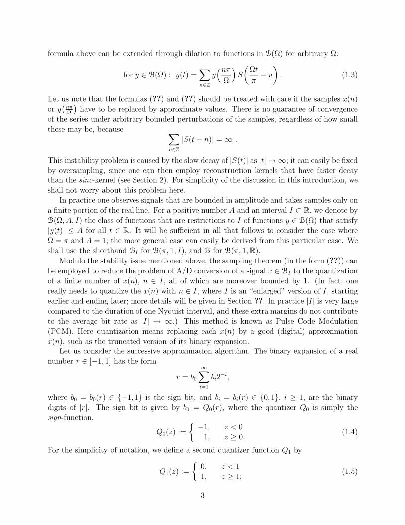
Let us consider the successive approximation algorithm. The binary expansion of a real

number r ∈ [−1, 1] has the form

r = b0

∞∑

i=1

bi2−i,

where b0 = b0(r) ∈ −1, 1 is the sign bit, and bi = bi(r) ∈ 0, 1, i ≥ 1, are the binary

digits of |r|. The sign bit is given by b0 = Q0(r), where the quantizer Q0 is simply the

sign-function,

Q0(z) :=

−1, z < 0

1, z ≥ 0.(1.4)

For the simplicity of notation, we define a second quantizer function Q1 by

Q1(z) :=

0, z < 1

1, z ≥ 1;(1.5)

3

zi - + -

ui−bi

HHH2 -

ui+1q

Q1

-q bi+1

+ –?

Delay

6

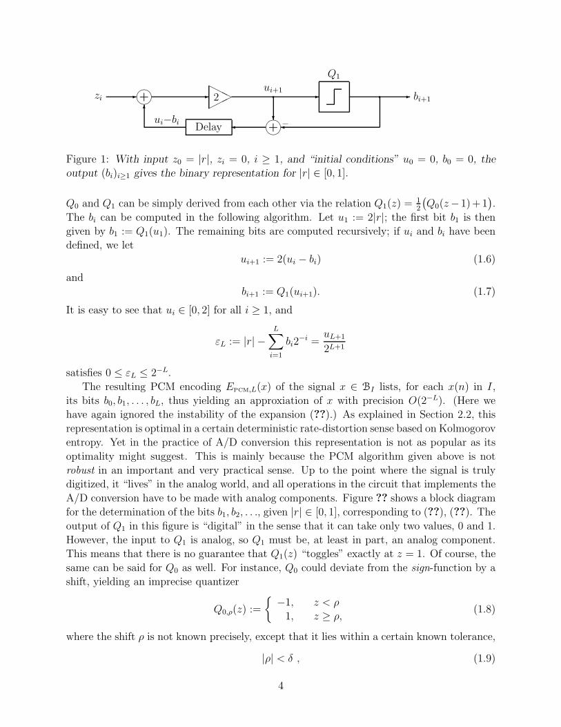
Figure 1: With input z0 = |r|, zi = 0, i ≥ 1, and “initial conditions” u0 = 0, b0 = 0, the

output (bi)i≥1 gives the binary representation for |r| ∈ [0, 1].

Q0 and Q1 can be simply derived from each other via the relation Q1(z) = 12

(

Q0(z−1)+1)

.

The bi can be computed in the following algorithm. Let u1 := 2|r|; the first bit b1 is then

given by b1 := Q1(u1). The remaining bits are computed recursively; if ui and bi have been

defined, we let

ui+1 := 2(ui − bi) (1.6)

and

bi+1 := Q1(ui+1). (1.7)

It is easy to see that ui ∈ [0, 2] for all i ≥ 1, and

εL := |r| −L∑

i=1

bi2−i =

uL+1

2L+1

satisfies 0 ≤ εL ≤ 2−L.

The resulting PCM encoding EPCM,L(x) of the signal x ∈ BI lists, for each x(n) in I,

its bits b0, b1, . . . , bL, thus yielding an approxiation of x with precision O(2−L). (Here we

have again ignored the instability of the expansion (??).) As explained in Section 2.2, this

representation is optimal in a certain deterministic rate-distortion sense based on Kolmogorov

entropy. Yet in the practice of A/D conversion this representation is not as popular as its

optimality might suggest. This is mainly because the PCM algorithm given above is not

robust in an important and very practical sense. Up to the point where the signal is truly

digitized, it “lives” in the analog world, and all operations in the circuit that implements the

A/D conversion have to be made with analog components. Figure ?? shows a block diagram

for the determination of the bits b1, b2, . . ., given |r| ∈ [0, 1], corresponding to (??), (??). The

output of Q1 in this figure is “digital” in the sense that it can take only two values, 0 and 1.

However, the input to Q1 is analog, so Q1 must be, at least in part, an analog component.

This means that there is no guarantee that Q1(z) “toggles” exactly at z = 1. Of course, the

same can be said for Q0 as well. For instance, Q0 could deviate from the sign-function by a

shift, yielding an imprecise quantizer

Q0,ρ(z) :=

−1, z < ρ

1, z ≥ ρ,(1.8)

where the shift ρ is not known precisely, except that it lies within a certain known tolerance,

|ρ| < δ , (1.9)

4

where δ > 0 is fixed; moreover, its value may differ from one application to the next. More

generally, Q0 could be replaced by a “flaky” version Qf0,δ for which we know only that

Qf0,δ(z) :=

−1, z ≤ −δ

1, z ≥ δ

−1 or 1, z ∈ (−δ, δ).

(1.10)

This notation means that for each z, the flaky quantizer Qf0,δ will assign a value in −1, 1,

but that for z ∈ (−δ, δ) we just do not know what that value will be; moreover, if Qf0,δ

acts on the same z in (−δ, δ) in two different instances, it need not assign the same value

both times. We could model this by a (possibly input-dependent) probability distribution

on −1, 1, but since our results will hold for any such distribution, however ill-behaved, it

is easier to stick to (??). The imprecise versions of Q1 are, in the first case,

Q1,ρ(z) :=

0, z < 1 + ρ

1, z ≥ 1 + ρ,(1.11)

where ρ is constrained only by (??), and in the “flaky” case,

Qf1,δ(z) :=

0, z ≤ 1 − δ

1, z ≥ 1 + δ

0 or 1, z ∈ (1 − δ, 1 + δ).

(1.12)

We define Qf0,0 = Q0 and Qf

1,0 = Q1.

The debilitating effect of the quantization error can make itself felt in every bit, even

as early as b0 or b1. Assume, for example, that we are working with Q1,ρ, with ρ > 0. If

|r| ∈(

12, 1+ρ

2

)

, then b1(r) will be computed to be 0, which is incorrect since |r| > 12. No matter

how the remaining bits are assigned, the difference between r and the number represented

by the computed bits will be at least |r| − 12, which can be as large as ρ

2, and effectively as

large as δ2

by (??). This could easily translate to a uniform error of magnitude δ2, as it would

happen for the constant function x(t) ≡ r and for the scaled sinc-function x(t) = rS(t). A

similar anomaly can of course occur with the sign bit b0, too, if it is determined via Q0,ρ

rather than Q0: for r ∈ [0, ρ), the sign bit b0(r) will be incorrectly assigned, causing an error

that may be as large as δ.

In this paper, we present a study of different encoding schemes, and see how they trade

off accuracy for robustness. In Section 2, we define a framework for the discussion of our

different coders, and we carry out a more systematic analysis of PCM, its optimality and

its lack of robustness. Next we discuss two other schemes: the first one, in Section 3, is the

Sigma-Delta modulation; the second, in Section 4, replaces the binary expansion in PCM by

an expansion in a fractional base β ∈ (1, 2). We will show that both schemes are robust, in

the sense that even if the quantizer used to derive the digital representations is imperfect, it

is possible to reconstruct the signals with arbitrarily small error by taking more and more

bits from their digital representations; neither of them is optimal in the bit-rate, however.

Sigma-Delta modulation is well-known and popular in A/D conversion [?, ?, ?]; fractional

5

base expansions are less common, but also have been considered before, e.g., in [?]. In

both cases, robustness is linked to the fact that there is a certain amount of redundancy in

the codewords produced by these algorithms. It is this interplay between redundancy and

robustness that constitutes the major theme of this paper.

2 Encoding-Decoding, Kolmogorov ǫ-Entropy and Ro-

bustness

2.1 The average Kolmogorov ǫ-entropy of B

Let B be the space of our signals, as defined in Section ??. By an encoder E for BI we mean

a mapping

E : BI → Bwhere the elements in B are finite bitstreams. The result of the encoding is to take the

analog signal x to the digital domain. We also have a decoder D that maps bitstreams to

signals

D : B → CI

where CI denotes the space of continuous functions on I. Note that we may consider many

decoders D associated to a given E, and vice versa.

In general DEx 6= x. We can measure the distortion in the encoding-decoding by

‖x − DEx‖

where ‖ · ‖ is a norm defined on the signals of interest. We shall restrict our attention to the

norm

‖x‖CI:= ‖x‖L∞(I) := sup

t∈I|x(t)|.

One way of assessing the performance of an encoder-decoder pair (E, D) is to measure

the worst-case distortion for the class BI , defined by

d(BI ; E, D) := supx∈BI

‖x − DEx‖L∞(I).

In order to have a fair competition between various encoding-decoding schemes, we can look

at the performance as a function of the bit-cost. We define the bit-cost of an encoder E on

the space BI by

n(E, BI) := supx∈BI

#(Ex),

where #(Ex) is the number of bits in the bitstream Ex. Given a distortion tolerance ǫ > 0,

we let Cǫ(BI) denote the class of encoders E : BI → B for which there exists a decoder

D : B → CI such that d(BI ; E, D) ≤ ǫ. The smallest number of bits that can realize the

distortion ǫ for BI is then given by

nǫ(BI) := infE∈Cǫ(BI )

n(E, BI). (2.1)

6

It is well known that nǫ(BI) is determined by the Kolmogorov ǫ-entropy Hǫ(BI , CI) of

the class BI as a subset of CI . Here Hǫ(BI , CI) := log2 Nǫ(BI) where N := Nǫ(BI) is the

smallest number of functions f1, . . . , fN in CI forming an ǫ-net for BI , i.e., for each x ∈ BI

there exists an element fi in this collection such that ‖x − fi‖∞ ≤ ǫ. (In other words, N is

the smallest number of balls in CI , with radius ǫ in the ‖ · ‖∞-norm, that can cover BI .) The

number Nǫ(BI) is finite because the space BI is a compact subset of (CI , ‖ · ‖∞). It is then

easy to see that

nǫ(BI) = ⌈log2 Nǫ(BI)⌉ = ⌈Hǫ(BI , CI)⌉ (2.2)

with ⌈y⌉ denoting the smallest integer ≥ y. Indeed, an encoder-decoder pair with bit-

cost ⌈log2 Nǫ(BI)⌉ can easily be given: use the ⌈log2 Nǫ(BI)⌉ bits to label the functions

fi, 1 ≤ i ≤ Nǫ(BI) and assign each function x ∈ BI to the label of the nearest fi. On the

other hand, nǫ(BI) cannot get any smaller because otherwise one could construct an ǫ-net

via the same method with fewer elements than Nǫ(BI).

In many applications in signal processing, the interval I on which one wishes to recover

the signals x ∈ BI is varying, and |I| is large relative to the Nyquist sample spacing. In

the case of audio signals, sampling at 44, 000 times per second corresponds to high quality

audio, and sampling at 8, 000 times per second corresponds to wireless voice applications.

Recovering m minutes of such a signal means that the interval I corresponds to a number of

2, 640, 000m or 480, 000m consecutive samples, respectively. So, the interval I, while finite,

is typically very large. Given a family of encoders E = EII , defined for all intervals I, we

define the average bit-cost (i.e., bit rate) of this family to be

n(E) := lim sup|I|→∞

n(EI , BI)

|I| . (2.3)

The optimal encoding efficiency for the space B can be measured by the optimal average bit

rate that can be achieved within distortion ǫ. More formally, we define the quantity

nǫ(B) := lim|I|→∞

nǫ(BI)

|I| . (2.4)

There is a corresponding concept of average ǫ-entropy (per unit interval) of B, given by

Hǫ(B) := lim|I|→∞

Hǫ(BI , CI)

|I| . (2.5)

It easily follows from (??) that

nǫ(B) = Hǫ(B). (2.6)

The average ǫ-entropy of the class B can be derived from results of Kolmogorov and

Tikhomirov [?] on the average ǫ-entropy of certain classes of analytic functions. These

results yield

Hǫ(B) = (1 + o(1)) log2

1

ǫ, 0 < ǫ < 1. (2.7)

7

2.2 PCM encoders achieve the Kolmogorov ǫ-entropy

The Kolmogorov ǫ-entropy can be defined for any pair (F, V), where F is a compact subset

of the metric space V. Even when Hǫ(F, V) can be computed explicitly, we may not know

of any constructive example of an encoder-decoder pair that achieves (or near-achieves) the

Kolmogorov entropy. However, in the present case, where F = BI , V = CI , and we are

interested in Hǫ(BI , CI) when |I| is large (or equivalently, Hǫ(B) defined by the limit (??)),

the PCM encoding scheme does achieve (arbitrarily nearly) the optimal bit rate nǫ(B). This

is shown by the following argument, which uses methods that are similar to those used in

[?], with more generality.

The first issue to be taken care of is the instability of the expansion (??), as stated in

Section ??. We can circumvent this problem easily in the following way. We choose a real

number λ > 1 and sample x(t) at the points tn = n/λ, n ∈ Z, thereby obtaining the sequence

xn := x(nλ), n ∈ Z. When we reconstruct x from these sample values, we have more flexibility

since the sample values are redundant. If ϕ is any function such that its Fourier transform

ϕ satisfies

ϕ(ξ) =

1, |ξ| ≤ π

0, |ξ| ≥ λπ,(2.8)

and is sufficiently smooth for |ξ| ∈ [π, λπ], then we have the uniformly convergent recon-

struction formula (see, e.g., [?, p. 10] when ϕ is a Schwartz function, or [?])

x(t) =1

λ

∑

n∈Z

xnϕ(

t − n

λ

)

. (2.9)

Let the sequence of numbers Cn,λ(ϕ), n ∈ Z, be defined by

Cn,λ(ϕ) := sup0≤t< 1

λ

∣

∣

∣ϕ(

t − n

λ

)∣

∣

∣. (2.10)

Note that since ϕ is compactly supported, ϕ is infinitely differentiable. If, moreover, ϕ is

chosen to be twice differentiable, then |ϕ(t)| = O(|t|−2); therefore we have

Cλ(ϕ) :=∑

n∈Z

Cn,λ(ϕ) < ∞. (2.11)

For each λ > 1, let Fλ be the class of reconstruction kernels ϕ such that (??) and (??) hold.

We restrict ourselves to the class

F :=⋃

λ>1

Fλ.

Next, we define a family of PCM encoding-decoding pairs. For each real number λ > 1, we

select an arbitrary reconstruction filter ϕλ ∈ Fλ. We set Cn,λ := Cn,λ(ϕλ) and Cλ := Cλ(ϕλ).

For any interval I = [a, b], let Iλ,m := [a − M, b + M ] where M := Mλ,m is chosen so that

∑

|n|≥λM

Cn,λ ≤ 2−mCλ. (2.12)

8

We define the encoder EPCM := EPCM(I, λ, m) by its output

EPCM x :=

bi(xn) , i = 0, . . . , m, n/λ ∈ Iλ,m, n ∈ Z

for x ∈ BI . On the other hand, we define the output of the decoder DPCM to be

x(t) :=1

λ

∑

n∈λIλ,m

[xn]mϕλ

(

t − n

λ

)

, (2.13)

where we use the shorthand

[r]m := b0(r)

m∑

i=1

bi(r)2−i.

We can easily bound the distortion for this encoding-decoding. Decompose the error

signal x − x into two components as

x − x = e1 + e2,

where

e1(t) :=1

λ

∑

n∈λIλ,m

(xn − [xn]m)ϕλ

(

t − n

λ

)

and

e2(t) :=1

λ

∑

n 6∈λIλ,m

xnϕλ

(

t − n

λ

)

.

For the first error component, we use the sample error bound |xn − [xn]m| ≤ 2−m together

with the bound λ > 1 to obtain

|e1(t)| ≤ 2−m∑

n∈λIλ,m

∣

∣

∣ϕλ

(

t − n

λ

)∣

∣

∣≤ 2−m

∑

n∈Z

Cn,λ ≤ 2−mCλ.

Similarly for the second component, we note that t ∈ I and n 6∈ λIλ,m implies |t − nλ| ≥ M

so that

|e2(t)| ≤∑

n 6∈λIλ,m

∣

∣

∣ϕλ

(

t − n

λ

)∣

∣

∣≤

∑

|k|≥λM

Ck,λ ≤ 2−mCλ.

Putting these two estimates together we obtain

‖x − x‖L∞(I) ≤ Cλ2−m+1 (2.14)

uniformly for all x ∈ B. The number of bits n(EPCM(I, λ, m), BI) used in this encoding

satisfies the bound

n(EPCM(I, λ, m), BI) ≤⌈

λ|Iλ,m|(m + 1)⌉

=⌈

λ(|I| + 2M)(m + 1)⌉

.

Apart from I, note that these encoders have two parameters, λ and m. Given any ǫ > 0,

we now choose λ = λǫ and m = mǫ as follows: We first define the set

Λǫ :=

λ : log2(8Cλ) ≤(

log2

1

ǫ

)1/2

;

9

here the function(

log21ǫ

)1/2can be replaced by any other function that is o

(

log21ǫ

)

but still

diverges to ∞ as ǫ → 0. Note that Λǫ ⊃ Λǫ′ if ǫ < ǫ′ and⋃

ǫ>0

Λǫ = limǫ→0

Λǫ = (1,∞).

In particular, Λǫ is nonempty for all sufficiently small ǫ. We can therefore select λǫ ∈ Λǫ

such that λǫ → 1 as ǫ → 0; in other words, we have

λǫ = 1 + o(1) (2.15)

and

log2(8Cλǫ) ≤

(

log2

1

ǫ

)1/2

. (2.16)

We next define mǫ to be

mǫ := min

m ∈ N : Cλǫ2−m+1 ≤ ǫ

. (2.17)

The definition of mǫ and the bound (??) imply that EPCM(I, λǫ, mǫ) belongs to the

class Cǫ(BI) of encoders that achieve maximum distortion ǫ for all I. Denoting the family

EPCM(I, λǫ, mǫ)I by E[ǫ]PCM, we have

n(E[ǫ]PCM) := lim sup

|I|→∞

n(EPCM(λǫ, mǫ), BI)

|I| ≤ λǫ(mǫ + 1). (2.18)

By definition of mǫ, we know that

Cλǫ2−mǫ+1 ≤ ǫ < Cλǫ

2−mǫ+2;

hence

mǫ + 1 ≤ log2

(

8Cλǫ

ǫ

)

≤ log2

1

ǫ+

(

log2

1

ǫ

)1/2

= (1 + o(1)) log2

1

ǫ.

This implies, together with (??) and (??), that

n(E[ǫ]PCM) ≤ (1 + o(1)) log2

1

ǫ;

thus PCM encoders achieve the Kolmogorov entropy given by (??).

2.3 Robustness

As explained in Section ??, circuit implementation of A/D conversion, regardless of what

encoding scheme is used, necessarily incorporates at least one encoding step that makes a

transition from analog values to a discrete range, and that is accompanied by some “un-

certainty”. In other words, the encoder used by the A/D convertor is not known exactly;

rather, it can be any element of a restricted class E of encoders (corresponding to the different

values of the parameters within the uncertainty interval). We therefore have an additional

10

distortion in the encoding+decoding procedure that is due to our inability to know precisely

which encoder E in E was used for the encoding. For the decoding, we use the same decoder

for the whole class E . In analogy with the analysis in section 2.1 we introduce then

d(BI ; E , D) := supE∈E

d(BI , E, D) = supE∈E

supx∈BI

‖x − DEx‖∞ .

The bit cost for E is now defined by

n(E , BI) := supE∈E

n(E, BI) = supE∈E

supx∈BI

#(Ex) .

To generalize (??), we must minimize the bit cost for E over the choices (E , D). This requires

that we have several possible E at our disposal. Suppose that for each encoding algorithm

for BI we can identify the components that have to be analog, and the realistic tolerances

on their parameters, within e.g. a fixed $-budget for the construction of the corresponding

circuit. Then each combination (algorithm and parameter-tolerances) defines a family E .

Define Eτ to be the set of all these families, where the shorthand τ stands for the tolerance

limits imposed by the analog components. Then the minimum bit-cost that can achieve

distortion ǫ for a given parameter tolerance level τ is

nǫ,τ(BI) := infn(E , I); ∃D : B → BI and ∃E ∈ Eτ so that d(BI ; E , D) ≤ ǫ .

By definition, we have nǫ,τ (BI) ≥ nǫ(BI).

There is a fundamental difference between nǫ(BI) and nǫ,τ(BI) in the following sense.

The encoders E over which the infimum is taken to obtain nǫ(BI) can be viewed as just

abstract maps from BI to B. On the other hand, in order to define the classes E over which

we have to optimize to define nǫ,τ (BI), we have to consider a concrete implementation for

each encoder E and consider the class of its variations within realistic constraints on the

analog components. For this reason, unlike nǫ(BI) which was closely related to Kolmogorov

entropy, it is not straightforward how to relate nǫ,τ (BI) to a more geometric quantity. Even

so, it continues to make sense to define an average bit-cost,

nǫ,τ (B) = lim|I|→∞

nǫ,τ (BI)

|I| ,

and to consider its behavior as a function of ǫ.

In what follows, we shall consider the special class Eτ in which every E is constructed

as follows. We start from an encoder E along with an algorithmic implementation of it.

We denote this pair together by (E, b), where b stands for the “block diagram”, i.e., the

algorithm, that is used to implement E. We assume that b contains one or more quantizers

of type (??) or (??) but no other types of quantizers (all other operations are continuous).

We then consider all the encoders that have the same block diagram b, but with Q0 or Q1

replaced by a Q0,ρ or Q1,ρ (see (??, ??)) with |ρ| < δ, or by Qf0,δ or Qf

1,δ (see (??, ??)). We

call this class E[E,b,δ], and we define E [δ] to be the set of all E[E,b,δ] for which the encoder E

maps BI to B, and has an implementation with a block diagram b that satisfies the criteria

11

above. We can then define nǫ,[δ](BI) and nǫ,[δ](B) to be nǫ,τ(BI) and nǫ,τ(B), respectively,

for the choice Eτ = E [δ].

For the PCM encoder EPCM defined above in (??, ??), the substitution of Q0,ρ for Q0,

with |ρ| < δ and δ > 0, leads to (see the examples given at the end of the Introduction)

d(BI ; E[PCM,δ], D) ≥ δ ,

for every decoder D, regardless of how many bits we allow in the encoding. Consequently,

for ǫ < δ, it is impossible to achieve d(BI ; E[PCM,δ], D) ≤ ǫ. It follows that considering E[PCM,δ]

does not lead to a finite upper bound for nǫ,[δ](BI) or the average nǫ,[δ](B) when ǫ < δ; hence

the PCM-encoder is not “robust”.

In the next two sections we discuss two pairs (E, b) that are robust, in the sense that

they can achieve d(BI ; E[E,b,δ], D) ≤ ǫ for arbitrarily small ǫ > 0, regardless of the value of δ,

provided an extra number of bits is spent, compared to what is dictated by the Kolmogorov

entropy. Both constructions will provide us with finite upper bounds for nǫ,[δ](BI) and

nǫ,[δ](B). Our purpose next is to study how small these quantities can be made.

3 The Error Correction of Sigma-Delta Modulation

In this section, we shall consider encoders given by Sigma-Delta (Σ∆) Modulation; these

behave differently from PCM when imprecise quantization is used. We start by describing

the simplest case of a first order Σ∆ encoder E, i.e. the case where the quantizer is given

by the unperturbed (??). Then we show that this encoder is robust, in contrast to the PCM

encoder: if we replace the precise quantizer of (??) by a quantizer of type (??) , then the

encoding can nevertheless be made arbitrarily accurate. This leads to a discussion of what

we can conclude from this example, and from others in [?][?], about nǫ,[δ](BI) and nǫ,[δ](B).

3.1 First order Σ∆ modulation with a precise quantizer

We again choose λ > 1 (although now we are interested in the limit λ → ∞ rather than

λ → 1). We continue with the notation xn := x(nλ) as above. Given (xn)n∈Z, the algorithm

creates a bitstream (bn)n∈Z, where bn ∈ −1, 1, whose running sums track those of xn.

There is an auxiliary sequence (un)n∈Z which evaluates the error between these two running

sums. Given the interval of interest I = [a, b], we take un = 0 for nλ

< (a − M), where

M := Mλ is to be specified later. For nλ∈ Iλ = [a − M, b + M ], we define

un+1 := un + xn − bn , (3.1)

where

bn := Q0(un) , (3.2)

and Q0 is the quantizer defined by (??). The Σ∆ encoder EΣ∆ := EΣ∆(I, λ) maps x to the

bitstream (bn)n∈Z. We see that EΣ∆ appropriates one bit for each sample, which corresponds

12

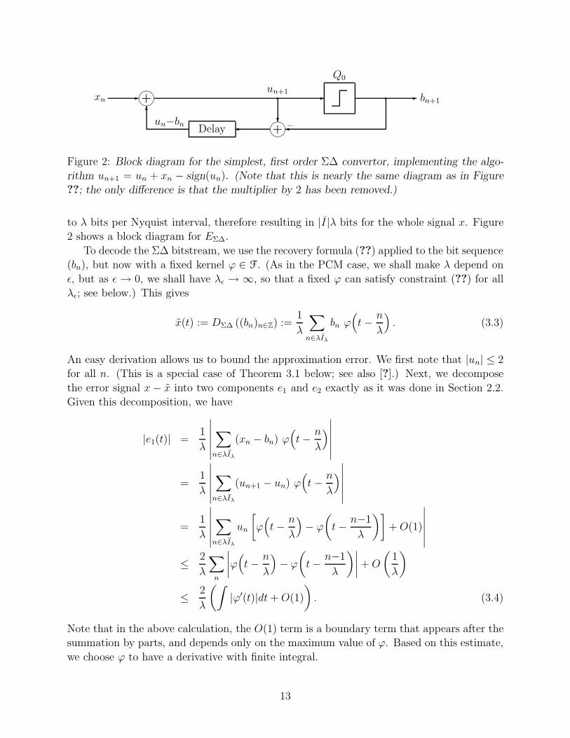
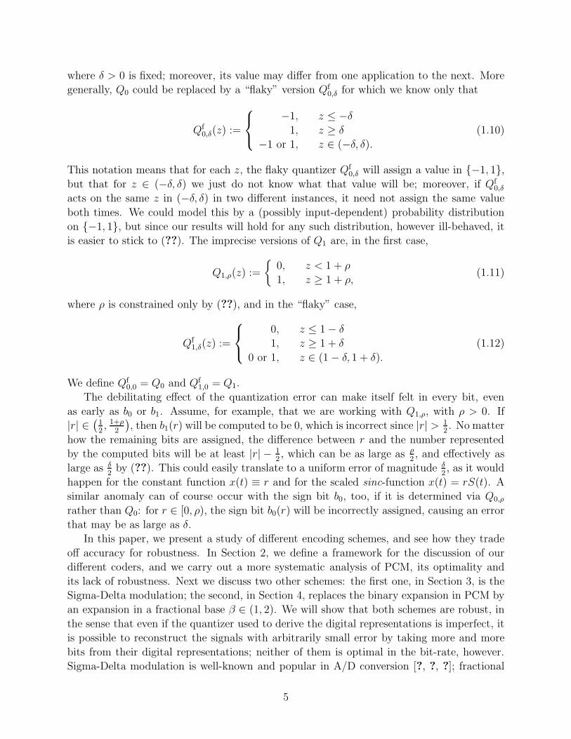
xn - + -

un−bn

un+1q

Q0

-q bn+1

+ –?

Delay

6

Figure 2: Block diagram for the simplest, first order Σ∆ convertor, implementing the algo-

rithm un+1 = un + xn − sign(un). (Note that this is nearly the same diagram as in Figure

??; the only difference is that the multiplier by 2 has been removed.)

to λ bits per Nyquist interval, therefore resulting in |I|λ bits for the whole signal x. Figure

2 shows a block diagram for EΣ∆.

To decode the Σ∆ bitstream, we use the recovery formula (??) applied to the bit sequence

(bn), but now with a fixed kernel ϕ ∈ F. (As in the PCM case, we shall make λ depend on

ǫ, but as ǫ → 0, we shall have λǫ → ∞, so that a fixed ϕ can satisfy constraint (??) for all

λǫ; see below.) This gives

x(t) := DΣ∆ ((bn)n∈Z) :=1

λ

∑

n∈λIλ

bn ϕ(

t − n

λ

)

. (3.3)

An easy derivation allows us to bound the approximation error. We first note that |un| ≤ 2

for all n. (This is a special case of Theorem 3.1 below; see also [?].) Next, we decompose

the error signal x − x into two components e1 and e2 exactly as it was done in Section 2.2.

Given this decomposition, we have

|e1(t)| =1

λ

∣

∣

∣

∣

∣

∣

∑

n∈λIλ

(xn − bn) ϕ(

t − n

λ

)

∣

∣

∣

∣

∣

∣

=1

λ

∣

∣

∣

∣

∣

∣

∑

n∈λIλ

(un+1 − un) ϕ(

t − n

λ

)

∣

∣

∣

∣

∣

∣

=1

λ

∣

∣

∣

∣

∣

∣

∑

n∈λIλ

un

[

ϕ(

t − n

λ

)

− ϕ

(

t − n−1

λ

)]

+ O(1)

∣

∣

∣

∣

∣

∣

≤ 2

λ

∑

n

∣

∣

∣

∣

ϕ(

t − n

λ

)

− ϕ

(

t − n−1

λ

)∣

∣

∣

∣

+ O

(

1

λ

)

≤ 2

λ

(∫

|ϕ′(t)|dt + O(1)

)

. (3.4)

Note that in the above calculation, the O(1) term is a boundary term that appears after the

summation by parts, and depends only on the maximum value of ϕ. Based on this estimate,

we choose ϕ to have a derivative with finite integral.

13

We have not yet specified how we choose Mλ. It suffices to choose Mλ so that

∑

|n|≥λMλ

Cn,λ(ϕ) ≤ 1

(see Section 2.2 for the definition of Cn,λ(ϕ)); then we guarantee that

‖e2‖L∞(I) ≤1

λ

and thus

‖x − x‖L∞(I) ≤Cϕ

λ(3.5)

with the constant Cϕ depending only on the choice of ϕ. By choosing λǫ = ⌈Cϕ/ǫ⌉ it follows

that

n(E[ǫ]Σ∆) := lim sup

|I|→∞

n(EΣ∆(I, λǫ))

|I|

= lim|I|→∞

λǫ(|I| + 2Mλǫ)

|I|= λǫ

= (1 + o(1))Cϕ

ǫ, (3.6)

where E[ǫ]Σ∆ denotes the family of encoders EΣ∆(I, λǫ))I .

One may wonder if a better bit-rate can be given by improving the error estimate (??).

It is possible to improve the exponent of λ when the signal x is fixed, but not uniformly in

x. In fact, it follows from the analysis in [?] that there exists an absolute constant c > 0

such that

d(BI ; EΣ∆(I, λ), D) ≥ c

λ(3.7)

for every decoder D, linear or nonlinear.

We see in (??) that for an average bit rate λ, first order Σ∆ modulation results in an

accuracy that is much worse (inversely proportional to a power of λ) than what would be

achieved if PCM was used (exponential decay in λ). In other words, the bit rate changes

from logarithmic to linear in the reciprocal of the maximum allowable distortion. However,

Σ∆ encoders have the remarkable property to be impervious to imprecision in the quantizer

used in the circuit implementation; we shall see this next.

3.2 First order Σ∆ modulation with an imprecise quantizer

Suppose that in place of the quantizer Q0 of (??), we use the imprecise quantizer Qf0,δ of (??)

in the first order Sigma-Delta algorithm; i.e., we have the same block diagram as in Figure

2, but Q0 is replaced by Qf0,δ. (Note that this includes the case where Q0 is replaced by a

Q0,ρ where ρ can conceivably vary with n within the range [−δ, δ].) Using these quantizers

will result in a different bitstream than would be produced by using Q0. In place of the

14

auxiliary sequence un of (??), which would be the result of exact quantization, we obtain

the sequence ufn, which satisfies uf

n = 0 for nλ

< a − M and

ufn+1 = uf

n + xn − bfn, n ∈ λI (3.8)

where

bfn = Qf

0,δ(ufn).

Theorem ??, below, shows that if we are given any δ > 0, then the error of at most δ, in

each implementation of flaky quantization in the Σ∆ encoder, will not affect the distortion

bound (??) save for the constant C0.

Theorem 3.1 Suppose that Σ∆ modulation is implemented by using, at each occurence, a

quantizer Qf0,δ, with δ > 0, in place of Q0. If the sequence (bf

n)n∈λI is used in place of (bn)n∈λI

in the decoder (??), the result is a function xf which satisfies

‖x − xf‖L∞(I) ≤ Cδ,ϕλ−1 (3.9)

with Cδ,ϕ = Cϕ(1 + δ/2) and Cϕ the constant in (??) .

Proof: This theorem was proved in [?]. We do not repeat its simple proof in detail, but

give a sketch here. The main idea is to establish the following bound:

|ufn| ≤ 2 + δ; (3.10)

this can be proved by induction on n by the following argument. It is clear for n < λ(a−M).

Assume that (??) has been shown for n ≤ N . If ufN ≤ δ, then bf

N := −1. Consequently,

xN − bfN ∈ [0, 2] and hence uf

N+1 = ufN + xN − bf

N ∈ [−2 − δ, 2 − δ] ⊂ [−(2 + δ), 2 + δ].

A similar argument applies if ufN > δ. Finally, if |uf

n| < δ, then |xN − bfN | ≤ 2 implies

|ufN + xN − bf

N | ≤ 2 + δ. Therefore we have advanced the induction hypothesis. This proves

(??) for all n. The remainder of the proof uses summation by parts again to obtain (??)

(see [?]).

Hence, despite the use of a quantizer that is inherently inaccurate, we nevertheless ob-

tain an arbitrarily precise approximation to the original signal. The average bitrate of this

algorithm can be computed exactly as in subsection ??, leading to the estimate

nǫ,[δ](B) ≤ Cδ

ǫ,

where Cδ is the infimum of Cδ,ϕ over all admissable reconstruction filters ϕ.

We shall see next that this estimate can be improved significantly.

3.3 Higher order Σ∆ modulators

Higher order Σ∆ modulators provide faster decay of the reconstruction error as λ → ∞.

In [?], an explicit family of arbitrary order single-bit Σ∆ modulators is constructed with

the property that the reconstruction error is bounded above by O(λ−k) for a k-th order

15

modulator. (The k-th order modulator in this context corresponds to replacing the first

order recursion (??) by a k-th order recursion ∆kun = xn − bn, where the estimates follow

from a choice of bn that ensures that the un are uniformly bounded.)

Note that because of the single-bit quantization, the average bit-rate is still equal to

the sampling rate λ. The error bound O(λ−k) involves a hidden constant C ′k (for a fixed,

admissable filter ϕ). Following the same steps as in the first order case we can bound the

average bit-rate in terms of the error tolerance ǫ as

nǫ,[δ](B) ≤ C ′k1/k

ǫ−1/k .

One can still optimize this over k by adapting to ǫ. For this, one uses the quantitative bound

C ′k ≤ C ′′γk2

for some γ > 1 (see [?]), to conclude that

nǫ,[δ](B) ≤ infk

C ′k1/k

ǫ−1/k ≤ C ′′′2Γ√

log2(1/ǫ) , (3.11)

where Γ = 2√

log2(γ) > 0. Although this is an improvement over the bound we obtained

from the first order Σ∆ scheme, it is still a long way from the optimal average bitrate,

which, as we saw in section 2, is proportional to log2(1/ǫ). In the next subsection we shall

examine a different type of Σ∆ modulators constructed in [?] which employ filters that are

more general than pure integration. These modulators achieve exponential accuracy in the

bit-rate while being robust with respect to small quantization errors, hence yielding much

better bounds on the average bit-rate nǫ,[δ](B).

3.4 Exponentially accurate Σ∆ modulator with an imprecise quan-

tizer

The following result can be thought of as a generalization of the robustness result for the

first order Σ∆ algorithm.

Theorem 3.2 Let δ ≥ 0 and consider the nonlinear difference equation

un =∑

j≥1

hjun−j + xn − bn, n ≥ n0, (3.12)

where

bn = Qf0,δ

(

∑

j≥1

hjun−j + xn

)

, (3.13)

and |un| ≤ 1 + δ for n < n0. If (1 + δ)‖h‖1 + ‖x‖∞ + δ ≤ 2, then ‖u‖∞ ≤ 1 + δ.

Proof: The proof is by induction. Let the coefficients (hj)j≥1 and the input (xn) satisfy

(1 + δ)‖h‖1 + ‖x‖∞ + δ ≤ 2 and assume that |ul| ≤ 1 + δ for all l < n. Let wn =∑

j≥1 hjun−j + xn so that un = wn − bn. First, it is clear that

|wn| ≤ (1 + δ)‖h‖1 + ‖x‖∞ ≤ 2 − δ.

16

Without loss of generality, let δ > 0. Three cases appear:

• If wn ∈ [δ, 2 − δ], then bn = 1, so that un = wn − 1 ∈ [−1 + δ, 1 − δ].

• If wn ∈ [−2 + δ,−δ], then bn = −1, so that un = wn + 1 ∈ [−1 + δ, 1 − δ].

• If wn ∈ (−δ, δ), then |un| ≤ |wn| + |bn| < δ + 1, regardless of the value bn ∈ −1, 1 is

assigned by the flaky quantizer.

The case δ = 0 is similar except the last case does not exist.

In [?], a two-parameter family of Σ∆-filters h(k,σ) : k ∈ Z+, σ ∈ Z+ was designed that

achieves exponential accuracy in the bit-rate. More specifically, the following results hold:

(i) ‖h(k,σ)‖1 ≤ cosh(πσ−1/2) uniformly in k,

(ii) Let x ∈ B. Given any interval I and for each λ, if we set xn := x(n/λ), n ∈ λIλ as

before, and if bn satisfies (??) with h = h(k,σ), then

supt∈I

∣

∣

∣

∣

∣

∣

x(t) − 1

λ

∑

n∈λIλ

bnϕ(

t − n

λ

)

∣

∣

∣

∣

∣

∣

≤ ‖u‖∞(Cϕσk)kλ−k.

The exponential accuracy in λ is achieved by choosing, for each λ, the optimal order k. This

optimization results in the error bound

‖x − x‖L∞(I) ≤ C02−rλ

where r = r(σ) = 1/(σπ log 2) > 0.

Theorem ?? allows us now to achieve the same result with flaky quantizers. Let us say

that a Σ∆-filter h := (hj) is δ-tolerant for B(π, µ, R) if the stability condition of Theorem

?? is satisfied, i.e., if (1 + δ)‖h‖1 + µ + δ ≤ 2. Given µ < 1 and δ > 0, let σ0 = σ0(µ, δ) to

be the smallest positive integer σ such that

(1 + δ) cosh(πσ−1/2) + µ + δ ≤ 2.

It is easy to check that σ0 exists if and only if µ + 2δ < 1 and

σ0(µ, δ) =

⌈

[

1

πcosh−1

(

2 − µ − δ

1 + δ

)]−2⌉

.

Hence we deduce that the Σ∆-filters h(k,σ0), k ∈ Z+, are all δ-tolerant for B(π, µ, R). If for

each reconstruction error tolerance ǫ we choose λ = λǫ such that C02−r(σ0)λ = ǫ, then we

find that

nǫ,[δ](B(π, µ, R)) ≤ λǫ

= σ0(µ, δ)π lnC0

ǫ= [σ0(µ, δ)π log 2 + o(1)] nǫ(B). (3.14)

17

In this estimate, the smallest value of σ0 is found in the limit µ → 0 and δ → 0. A

simple calculation reveals this value to be 6; the corresponding minimum increase factor in

the average bit-rate (when this algorithm is used) is 6π log 2 ≈ 13.07.

The question arises whether there exist other redundant encoders which can achieve self

correction for quantization error and exponential accuracy in terms of the bit rate (with

possibly a better constant) by means of other approaches than heavy oversampling. In the

next section, we show that this is indeed the case. Not only will we obtain such encoders;

we will also show that they are asymptotically optimal in the limit as δ → 0.

4 Beta-Encoders with Error Correction

We shall now show that it is possible to obtain exponential bit rate performance while

retaining quantization error correction by using what we shall call beta-encoders1. These

encoders will introduce redundancy in the representation of the signals, but will, contrary to

Σ∆ modulation, start from samples at the Nyquist rate (or rather slightly over the Nyquist

rate to ensure stability). The essential idea is to replace the binary representation∑∞

i=1 bi2−i

of a real number y ∈ [0, 1) by a representation of type∑∞

i=1 biβ−i, where 1 < β < 2, and

where each of the bi can still take only the values 0 or 1. Introducing γ := 1/β, it is more

convenient to write

y =

∞∑

i=1

biγi . (4.1)

In fact there are many such representations; this redundancy will be essential to us.

4.1 Redundancy in beta-encoding

We start by showing one strategy that gives, for each y ∈ [0, 1], an assignment of bits, i.e.

values bi := bi(y) ∈ 0, 1, such that (??) is satisfied. Given y, we define u1 = βy, and we

set b1 = 1 if u1 ≥ 1, b1 = 0 if u1 < 1, i.e. b1 = Q1(u1), with Q1 as defined in (??). We then

proceed recursively for i ≥ 1, defining ui+1 = β(ui − bi) and bi+1 = Q1(ui+1). It is easy to

see that ui always lies in [0, β]. By the definition of the ui,

L∑

i=1

uiγi −

L∑

i=1

biγi =

L∑

i=1

(ui − bi)βγi+1 =L∑

i=1

ui+1γi+1 ,

so that from above,

L∑

i=1

biγi = γu1 − uL+1γ

L+1 = y − uL+1γL+1 ,

which implies, since uL+1 ∈ [0, β],

0 ≤ εL(y) := y −L∑

i=1

biγi ≤ γL.

1This name is motivated by the term β-expansion in [?].

18

The successive approximations∑L

i=1 biγi to y thus achieve an accuracy that decays ex-

ponentially in L, albeit slower than the usual binary successive approximations. In fact, the

algorithm is very similar to the binary successive approximation algorithm in subsection 2.2;

the only difference is the substitution of multiplication by β for the doubling operation we

had there.

Although we will be ultimately interested in applying this algorithm to numbers in [0, 1]

only, it is useful to note that it works just as well for numbers y in the larger interval

[0, (β−1)−1). In this case, one finds that the corresponding ui lie in [0, β(β−1)−1), resulting

in the bound

0 ≤ εL(y) < (β − 1)−1γL.

We can exploit this observation to define a different beta-expansion of y ∈ [0, 1], by the

following argument: If y < γ(β−1)−1, then we know, by the observation just made, that there

exists a bit sequence (dj)j∈N so that y = γ∑∞

j=1 djγj, yielding a beta-expansion of y whose

first bit is equal to zero. Motivated by this, let us set b1 = 0 if u1 := βy < (β−1)−1, and b1 = 1

if βy ≥ (β−1)−1. In either case, one checks easily that y−b1γ < γ(β−1)−1. (In the first case,

there is nothing to prove; in the second case, we have y−1 ≤ 1−γ = γ(β−1) < γ(β−1)−1.)

Since β(y−b1γ) < (β−1)−1, we can repeat the argument with y replaced by β(y−b1γ) =: γu2

to define b2 and so on. If we extend the definition of Q1 by setting Qν := 12[1 + Q0(· − ν)]

for ν ≥ 1, then we can write the above iteration explicitly as

u1 = βy

b1 = Q(β−1)−1(u1)

for i ≥ 1 : ui+1 = β(ui − bi) (4.2)

bi+1 = Q(β−1)−1(ui+1).

Because the resulting ui are all in the range [0, β(β − 1)−1), we still have the error bound

0 ≤ y −L∑

i=1

biγi < (β − 1)−1γL.

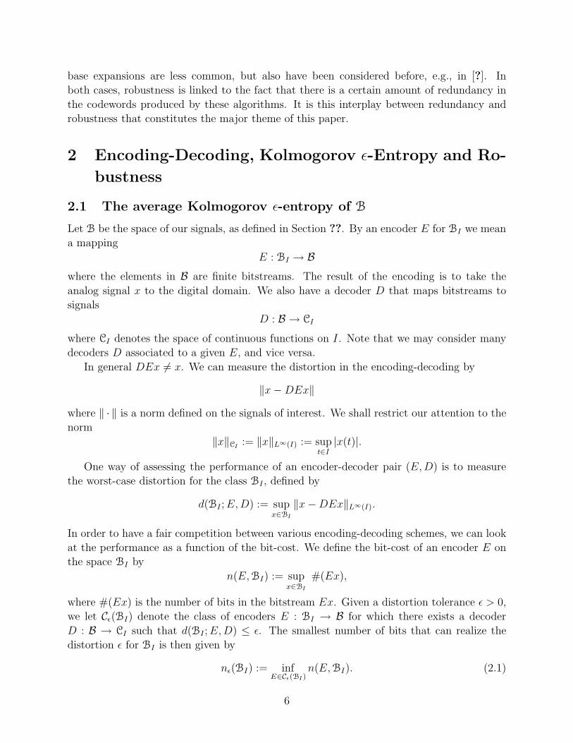
We can understand the difference between the two algorithms given so far by visualizing

the definitions of b1(y) and b1(y) as y increases from 0 to 1, as shown in Figure 3. As long

as y is smaller than γ, both algorithms keep the first bit equal to zero. However, if y is

greater than or equal to γ, then the first algorithm seizes its chance and allocates b1 = 1,

and starts over again with βy − 1. We call this algorithm “greedy” because the bits are

assigned greedily; in every iteration, given the first j bits b1, . . . , bj , the algorithm will set

bj+1 equal to 1 as long as γj+1 +∑j

i=1 biγi is less than y. The second algorithm does the

opposite: if it can get away with keeping b1 = 0, i.e., if y ≤∑∞

i=2 γi = γ(β − 1)−1, it is

content with b1 = 0; only when y exceeds this value, and hence the bi for i ≥ 2 would not

be able to catch up on their own, does this algorithm set b1 = 1. This approach is then

continued in the assignment of all the remaining bits. Because it only sets a bit equal to 1

when forced to do so, we call this algorithm the “lazy” algorithm.2 Laziness has its price:

2For some of the recent mathematical accounts of greedy and lazy expansions, see, e.g., [?], [?].

19

-bi = 0 -bi = 1

0

γ

γ(β − 1)−1 1 β β(β − 1)−1

- -bi = 0 bi = 1

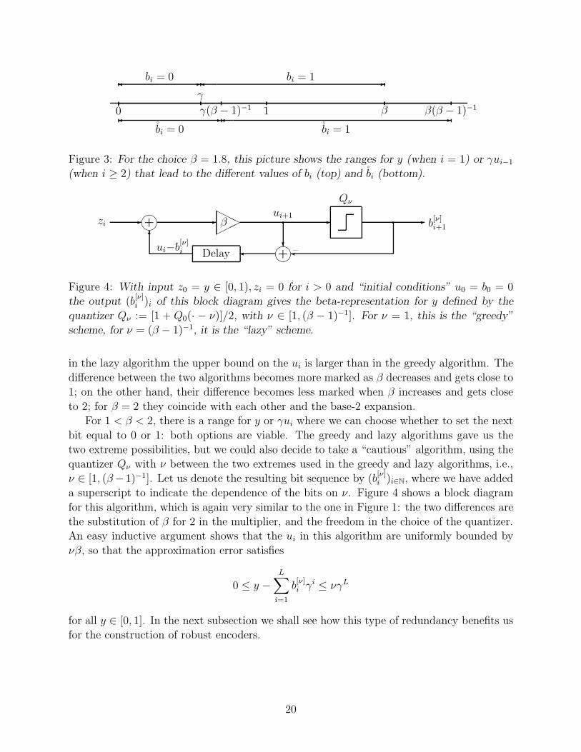
Figure 3: For the choice β = 1.8, this picture shows the ranges for y (when i = 1) or γui−1

(when i ≥ 2) that lead to the different values of bi (top) and bi (bottom).

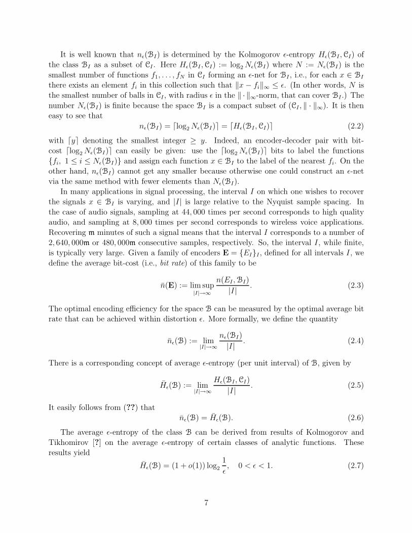
zi - + -

ui−b[ν]i

HHHβ -

ui+1q

Qν

-q b[ν]i+1

+ –?

Delay

6

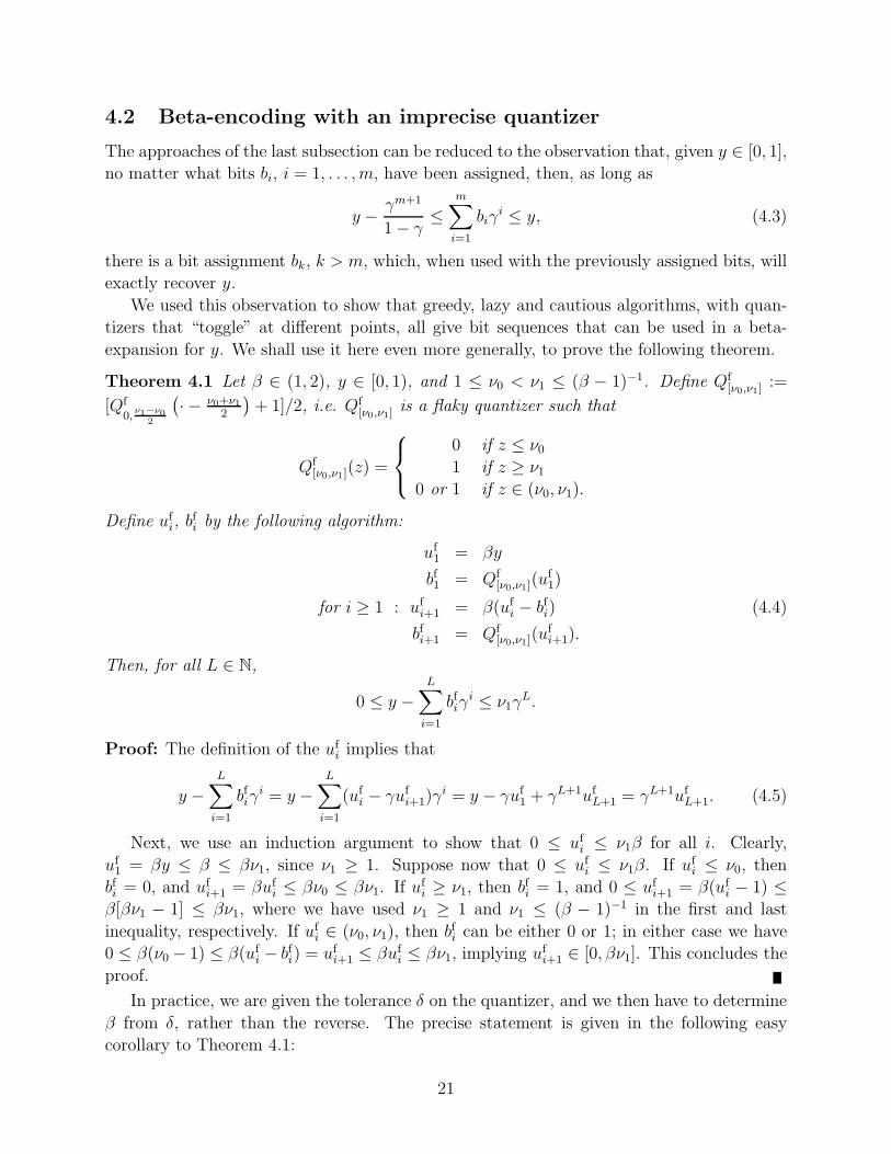
Figure 4: With input z0 = y ∈ [0, 1), zi = 0 for i > 0 and “initial conditions” u0 = b0 = 0

the output (b[ν]i )i of this block diagram gives the beta-representation for y defined by the

quantizer Qν := [1 + Q0(· − ν)]/2, with ν ∈ [1, (β − 1)−1]. For ν = 1, this is the “greedy”

scheme, for ν = (β − 1)−1, it is the “lazy” scheme.

in the lazy algorithm the upper bound on the ui is larger than in the greedy algorithm. The

difference between the two algorithms becomes more marked as β decreases and gets close to

1; on the other hand, their difference becomes less marked when β increases and gets close

to 2; for β = 2 they coincide with each other and the base-2 expansion.

For 1 < β < 2, there is a range for y or γui where we can choose whether to set the next

bit equal to 0 or 1: both options are viable. The greedy and lazy algorithms gave us the

two extreme possibilities, but we could also decide to take a “cautious” algorithm, using the

quantizer Qν with ν between the two extremes used in the greedy and lazy algorithms, i.e.,

ν ∈ [1, (β−1)−1]. Let us denote the resulting bit sequence by (b[ν]i )i∈N, where we have added

a superscript to indicate the dependence of the bits on ν. Figure 4 shows a block diagram

for this algorithm, which is again very similar to the one in Figure 1: the two differences are

the substitution of β for 2 in the multiplier, and the freedom in the choice of the quantizer.

An easy inductive argument shows that the ui in this algorithm are uniformly bounded by

νβ, so that the approximation error satisfies

0 ≤ y −L∑

i=1

b[ν]i γi ≤ νγL

for all y ∈ [0, 1]. In the next subsection we shall see how this type of redundancy benefits us

for the construction of robust encoders.

20

4.2 Beta-encoding with an imprecise quantizer

The approaches of the last subsection can be reduced to the observation that, given y ∈ [0, 1],

no matter what bits bi, i = 1, . . . , m, have been assigned, then, as long as

y − γm+1

1 − γ≤

m∑

i=1

biγi ≤ y, (4.3)

there is a bit assignment bk, k > m, which, when used with the previously assigned bits, will

exactly recover y.

We used this observation to show that greedy, lazy and cautious algorithms, with quan-

tizers that “toggle” at different points, all give bit sequences that can be used in a beta-

expansion for y. We shall use it here even more generally, to prove the following theorem.

Theorem 4.1 Let β ∈ (1, 2), y ∈ [0, 1), and 1 ≤ ν0 < ν1 ≤ (β − 1)−1. Define Qf[ν0,ν1]

:=

[Qf0,

ν1−ν0

2

(

· − ν0+ν1

2

)

+ 1]/2, i.e. Qf[ν0,ν1]

is a flaky quantizer such that

Qf[ν0,ν1]

(z) =

0 if z ≤ ν0

1 if z ≥ ν1

0 or 1 if z ∈ (ν0, ν1).

Define ufi, bf

i by the following algorithm:

uf1 = βy

bf1 = Qf

[ν0,ν1](uf1)

for i ≥ 1 : ufi+1 = β(uf

i − bfi) (4.4)

bfi+1 = Qf

[ν0,ν1](ufi+1).

Then, for all L ∈ N,

0 ≤ y −L∑

i=1

bfiγ

i ≤ ν1γL.

Proof: The definition of the ufi implies that

y −L∑

i=1

bfiγ

i = y −L∑

i=1

(ufi − γuf

i+1)γi = y − γuf

1 + γL+1ufL+1 = γL+1uf

L+1. (4.5)

Next, we use an induction argument to show that 0 ≤ ufi ≤ ν1β for all i. Clearly,

uf1 = βy ≤ β ≤ βν1, since ν1 ≥ 1. Suppose now that 0 ≤ uf

i ≤ ν1β. If ufi ≤ ν0, then

bfi = 0, and uf

i+1 = βufi ≤ βν0 ≤ βν1. If uf

i ≥ ν1, then bfi = 1, and 0 ≤ uf

i+1 = β(ufi − 1) ≤

β[βν1 − 1] ≤ βν1, where we have used ν1 ≥ 1 and ν1 ≤ (β − 1)−1 in the first and last

inequality, respectively. If ufi ∈ (ν0, ν1), then bf

i can be either 0 or 1; in either case we have

0 ≤ β(ν0 − 1) ≤ β(ufi − bf

i) = ufi+1 ≤ βuf

i ≤ βν1, implying ufi+1 ∈ [0, βν1]. This concludes the

proof.

In practice, we are given the tolerance δ on the quantizer, and we then have to determine

β from δ, rather than the reverse. The precise statement is given in the following easy

corollary to Theorem 4.1:

21

Corollary 4.2 Given δ > 0, define β = 1 + (2δ + 1)−1. Let y ∈ [0, 1] be arbitrary. Let

(bfi)i∈N be the bit sequence defined by the iteration (??), with ν0 = 1, ν1 = (β − 1)−1, i.e.,

Qf[ν0,ν1]

= [Qf0,δ(· − (1 + δ)) + 1]/2 = Qf

1,δ(· − δ). Then

0 ≤ y −m∑

i=1

bfiβ

−i ≤ (2δ + 1)β−m.

We have thus achieved the goal we set ourselves at the start of this section: we have an

algorithm that starts from samples at (slightly above) the Nyquist rate, and that has suffi-

cient redundancy to allow the use of an imprecise quantizer, without significantly affecting

the exponential accuracy in the number of bits that is achieved by using a precise quantizer

in the same algorithm. In the next subsection we look at the corresponding average bitrate.

4.3 Bitrate for beta-encoding with an imprecise quantizer

As in the PCM case, we start from (??). We want to have an accurate representation of a

signal x ∈ BI , with I = [a, b], starting from an imprecise beta-quantization of its samples.

We assume that δ > 0 is given, and we define β = 1 + (2δ + 1)−1. For given sampling rate

λ and number of bits per sample m, the encoder Eβ−PCM(λ, m) takes samples xn = x(

nλ

)

,

from the enlarged interval Iλ,m = [a − M, b + M ], where M = Mλ,m is chosen such that

(??) holds (with 2−m replaced by β−m). For each n ∈ λIλ,m, we compute the first m bits,

bfi, i = 1, . . . , m of the flaky beta-quantization, described in Corollary ??, of the numbers

yn = (1 + xn)/2 ∈ [0, 1], and we define

[xn]m := 2[yn]m − 1 := 2

(

m∑

i=1

bfiβ

−i

)

− 1,

x(t) =1

λ

∑

n∈λI

[xn]m ϕλ

(

t − n

λ

)

.

Then we obtain, analogously to the analysis in subsection ??, and using Corollary ??, the

error estimate

‖x − x‖L∞(I) ≤ Cλ(2δ + 2)β−m. (4.6)

As before, the total number of bits used to obtain this accuracy is bounded by ⌈m(2M +

|I|)λ⌉. For each ǫ > 0, we choose λ = λǫ and m = mǫ exactly in the same way as it was

done in subsection ?? (again replacing 2 by β wherever appropriate). This selection results

in the average bit-rate bound

n(E[ǫ]β−PCM) ≤ (1 + o(1)) logβ

1

ǫ,

or in other words, noting that β = 1 + (2δ + 1)−1,

nǫ,[δ](B) ≤(

log2

[

1 +1

2δ + 1

])−1

nǫ(B) . (4.7)

This estimate is a significant improvement over the result of subsection ?? in that first, it is

valid for all δ > 0, and second, it recovers the optimal bit-rate nǫ(B) in the limit as δ → 0.

22

5 Discussion

The two examples of robust encoders presented here exhibit a large amount of redundancy in

the representation of the signal x(t): many different bit sequences can in fact correspond to

the same signal. It is this feature that makes it possible to still obtain good approximations

even though the imprecise quantizers produce other bit sequences than the precise ones. This

suggests that in order to develop other schemes that may improve on the average bitrate

under imprecise analog-to-digital conversion, one has to build in redundancy from the start.

Although (??) is a significant improvement over (??), it would be suprising if it were

already optimal (for each δ). One could argue that, in some sense, “imprecise” quantizers

are similar to a noisy channel; one would then expect, by analogy with Shannon’s result,

that nǫ,[δ](B) = nǫ(B), even for arbitrary δ > 0 (as opposed to only in the limit for δ → 0, as

in (??)). We do not know whether this analogy is valid, and/or whether this equality holds.

It should be emphasized that all our results are asymptotic. The limit for |I| → ∞ is

fairly realistic, given the enormous difference in scale between the sampling period and the

duration in time of the signals of interest. The limits for very large λ (for Σ∆ modulation),

or λ very close to 1 (for β-encoders) are less realistic.

Finally, although the β-encoders give such a startling improvement in the average bit-rate,

it is clear that many other aspects have to be taken into account as well before this promise

can be realized in practice. In particular, analog implementations of the coder described in

subsection 4.3 are bound to have imprecise values of β as well as imprecise quantizers. (In

[?] it is shown how imprecise values of β can be taken into account as well.) Moreover, any

realistic approach should also take into account upper bounds, that are imposed a priori, on

all internal variables, such as the ui; this is in contrast with the upper bounds on the ui that

follow from the theoretical analysis, which may be too large to be possible in reality. The

analysis in this paper has not addressed any of these questions.

6 Summary

Nyquist rate A/D converters based on the successive approximation method are known to

be susceptible to component mismatch error, whereas Σ∆ modulators are not. An analysis

of the robustness of the Σ∆ modulator to component mismatch leads to the construction of

two alternate algorithms that achieve exponential bitrate (as opposed to a much slower rate

for simple Σ∆) yet are still robust under component mismatch. One of these algorithms is a

”filtered Σ∆ modulator”, with a appropriate filter; the other is a successive approximation

algorithm, based on the β-expansion of a number. Both are robust to circuit mismatch error.

The Kolmogorov rate-distortion framework is extended to incorporate component mismatch

error and the algorithms described provide upper bounds on what is ultimately achievable

within this framework.

23

References

[1] J. C. Candy, “A Use of Limit Cycle Oscillations to Obtain Robust Analog-to-Digital

Converters,” IEEE Trans. Commun. , vol. COM-22, No. 3, pp. 298-305, March 1974.

[2] C. C. Cutler, “Transmission System Employing Quantization,” U.S. Patent 2927962,

Mar. 8, 1960.

[3] I. Daubechies, R. DeVore, “Reconstructing a Bandlimited Function From Very Coarsely

Quantized Data: A Family of Stable Sigma-Delta Modulators of Arbitrary Order”, Ann.

of Math., vol. 158, no. 2, pp. 679–710, Sept. 2003.

[4] I. Daubechies, O. Yılmaz, preprint.

[5] C. S. Gunturk, “One-Bit Sigma-Delta Quantization with Exponential Accuracy,”

Comm. Pure Appl. Math., vol. 56, pp. 1608–1630, no. 11, 2003.

[6] H. Inose and Y. Yasuda, “A Unity Bit Coding Method by Negative Feedback,” Proc.

IEEE,, vol. 51, pp. 1524-1535, Nov. 1963.

[7] C. S. Gunturk, J. C. Lagarias, and V. A. Vaishampayan,“On the Robustness of Single-

Loop Sigma-Delta Modulation,” IEEE Trans. Inform. Th., vol. 47, No. 5, pp. 1735-1744,

July 2001.

[8] A. N. Karanicolas, H.-S. Lee and K. L. Bacrania, “A 15-b 1-Msample/s Digitally Self-

Calibrated Pipeline ADC”, IEEE Journal of Solid-State Circuits, vol. 28, No. 12, pp.

1207-1215, Dec. 1993.

[9] A. N. Kolmogorov and V. M. Tikhomirov, “ǫ-entropy and ǫ-capacity of sets in function

spaces,” Uspehi, 14(86):3-86, 1959 (also: AMS Translations, Series 2, Vol. 17, 1961, pp.

277-364).

[10] S. H. Lewis and P. R. Gray, “A Pipelined 5-Msample/s 9-bit Analog-to-Digital Con-

verter,” IEEE Journal of Solid State Circuits, vol. sc-22, No. 6, pp. 954-961, Dec. 1987.

[11] Y. Meyer, “Wavelets and Operators,” Cambridge University Press, 1992.

[12] W. Parry, “On β-expansions of real numbers,” Acta. Math. Acad. Sci. Hungar., vol. 15,

pp. 95-105, 1964.

[13] V. Komornik and P. Loreti, “Subexpansions, superexpansions and uniqueness properties

in non-integer bases,” Period. Math. Hungar. 44 (2002), no. 2, pp. 197–218.

[14] K. Dajani and C. Kraaikamp, “From greedy to lazy expansions and their driving dy-

namics,” Expo. Math., 20, (2002), no. 4, pp. 315–327.

24