Daubechies Wavelet/Scaling Filters: I -...
52
Daubechies Wavelet/Scaling Filters: I • orthonormality constraints on {h l } yield orthonormal W , but these alone are not sufficient to yield ‘reasonable’ MRA (i.e., one interpretable as a ‘scale by scale’ decomposition) • ‘regularity’ conditions lead to Daubechies wavelet filters • Daubechies {h l }’s defined via squared gain functions: H (D) (f ) ≡ 2 sin L (πf ) L 2 -1 X l =0 L 2 - 1+ l l cos 2l (πf ) - 2 sin L (πf ) ∝ squared gain for difference filter of order L/2 - 2nd part is squared gain for either ‘all-pass’ filter (L = 2) or low-pass filter (L =4, 6,...) with width L/2 WMTSA: 105–106 VI–1
-
Upload
truongtruc -
Category
Documents
-
view
237 -
download
0
Transcript of Daubechies Wavelet/Scaling Filters: I -...
Daubechies Wavelet/Scaling Filters: I
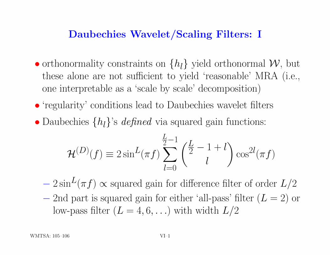
• orthonormality constraints on {hl} yield orthonormal W , butthese alone are not sufficient to yield ‘reasonable’ MRA (i.e.,one interpretable as a ‘scale by scale’ decomposition)
• ‘regularity’ conditions lead to Daubechies wavelet filters
• Daubechies {hl}’s defined via squared gain functions:
H(D)(f ) ≡ 2 sinL(πf )
L2−1∑l=0
(L2 − 1 + l
l
)cos2l(πf )
− 2 sinL(πf ) ∝ squared gain for difference filter of order L/2
− 2nd part is squared gain for either ‘all-pass’ filter (L = 2) orlow-pass filter (L = 4, 6, . . .) with width L/2
WMTSA: 105–106 VI–1
Daubechies Wavelet/Scaling Filters: II
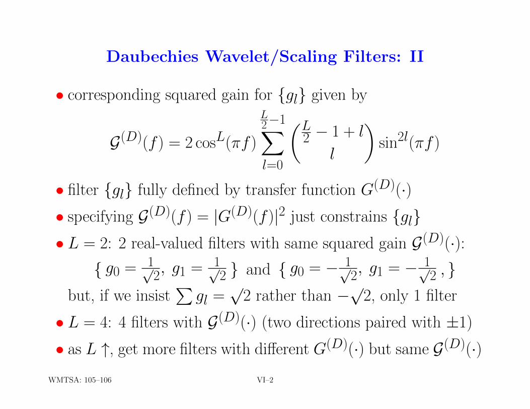
• corresponding squared gain for {gl} given by
G(D)(f ) = 2 cosL(πf )
L2−1∑l=0
(L2 − 1 + l
l
)sin2l(πf )
• filter {gl} fully defined by transfer function G(D)(·)• specifying G(D)(f ) = |G(D)(f )|2 just constrains {gl}• L = 2: 2 real-valued filters with same squared gain G(D)(·):
{ g0 = 1√2, g1 = 1√
2 } and { g0 = − 1√2, g1 = − 1√
2 , }but, if we insist
∑gl =
√2 rather than −
√2, only 1 filter
• L = 4: 4 filters with G(D)(·) (two directions paired with ±1)
• as L ↑, get more filters with different G(D)(·) but same G(D)(·)
WMTSA: 105–106 VI–2
Daubechies Wavelet/Scaling Filters: III
• can obtain all possible {gl} (and hence {hl}) systematicallyusing a procedure called ‘spectral factorization’
• Daubechies (1992) defined two classes of wavelets via criteriathat select a particular scaling filter {gl}• one criterion leads to ‘extremal phase’ class
• another criterion leads to ‘least asymmetric’ class
WMTSA: 106–107 VI–3
Extremal Phase Scaling Filters: I
• denote these filters by {g(ep)l }
• by definition, if {gl} and {g(ep)l } have same G(D)(·), then
m∑l=0
g2l ≤
m∑l=0
[g
(ep)l
]2for m = 0, . . . , L− 1
• summing up to m defines mth term of partial energy sequence
• partial energy builds up fastest for {g(ep)l } (‘front loaded’)
• note: above condition also called ‘minimum phase’
• filter of width L called D(L) scaling filter; e.g., D(4), D(6)
• {g(ep)l } for L = 4, 6, . . . , 20 are on course Web site
WMTSA: 106–109 VI–4
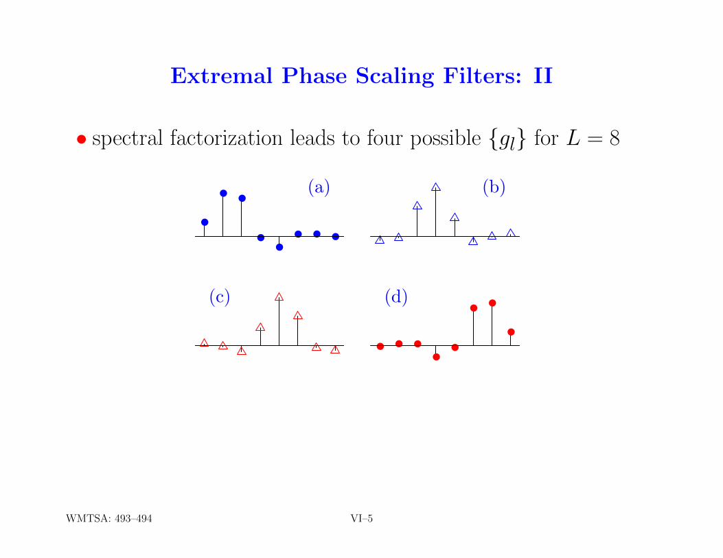
Extremal Phase Scaling Filters: II
• spectral factorization leads to four possible {gl} for L = 8
●
●●
●●
● ● ●
(a) (b)
(c)
● ● ●
●●
●●
●
(d)
WMTSA: 493–494 VI–5
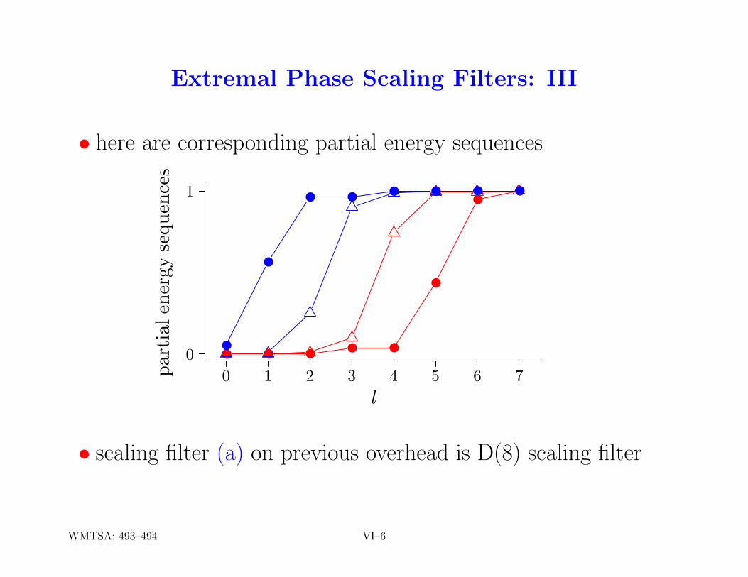
Extremal Phase Scaling Filters: III
• here are corresponding partial energy sequences
● ● ●● ●
●
●●
●
●
● ●● ● ● ●
0 1 2 3 4 5 6 70
1
l
part
ial e
nerg
y se
quen
ces
• scaling filter (a) on previous overhead is D(8) scaling filter
WMTSA: 493–494 VI–6
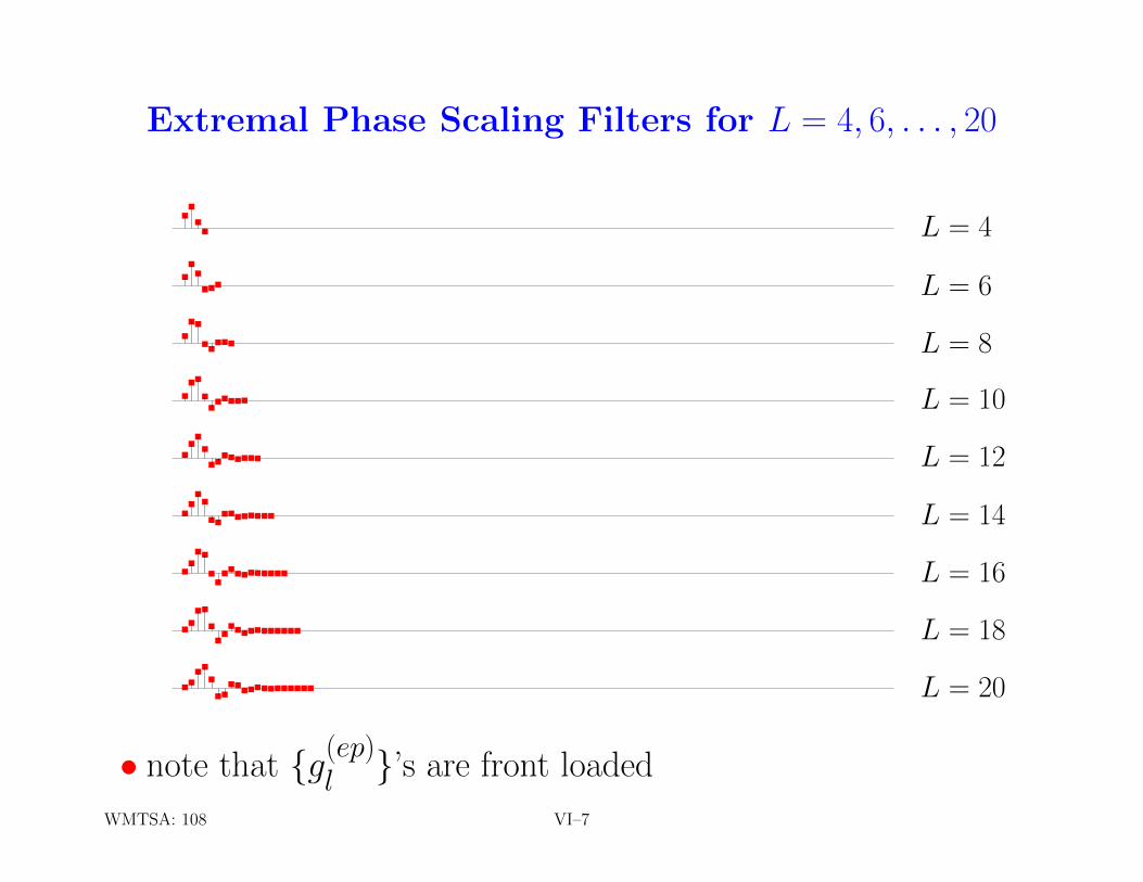
Extremal Phase Scaling Filters for L = 4, 6, . . . , 20
.
.
.
.
.
.
.
...
.
..
.....
.
..
.
......
.
..
.
........
.
.
.
.
..
........
.
.
..
.
.
..........
..
..
.
..
...........
..
..
.
..
.............
L = 4
L = 6
L = 8
L = 10
L = 12
L = 14
L = 16
L = 18
L = 20
• note that {g(ep)l }’s are front loaded
WMTSA: 108 VI–7
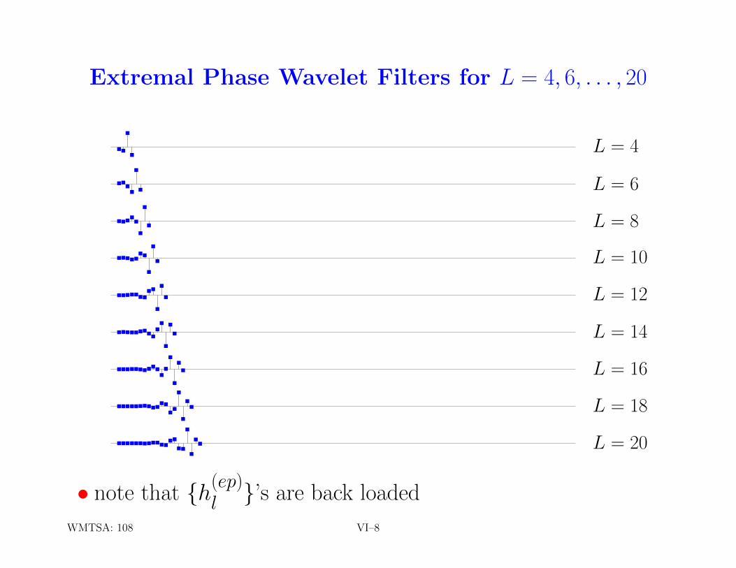
Extremal Phase Wavelet Filters for L = 4, 6, . . . , 20
..
.
.
...
.
.
.
.....
.
.
.
.....
..
.
.
.
.......
..
.
.
.
.........
.
.
.
.
.
..........
.
.
.
.
.
.
............
..
.
.
.
.
..............
..
.
.
..
L = 4
L = 6
L = 8
L = 10
L = 12
L = 14
L = 16
L = 18
L = 20
• note that {h(ep)l }’s are back loaded
WMTSA: 108 VI–8

D(4) Wavelet & Scaling Filters Revisited
..
.
.
....
.
.
.
.
..
........
....
.
...
......
........................
.
.....................
.
.
.
.
....
.
.....
........
........
......
.................................
.............
{h(ep)l }
{h(ep)2,l }
{h(ep)3,l }
{h(ep)4,l }
{g(ep)l }
{g(ep)2,l }
{g(ep)3,l }
{g(ep)4,l }
L = 4
L2 = 10
L3 = 22
L4 = 46
L = 4
L2 = 10
L3 = 22
L4 = 46
• jth level D(4) wavelet filters {h(ep)j,l }’s are back loaded, whereas
corresponding scaling filters {g(ep)j,l }’s are front loaded
VI–9
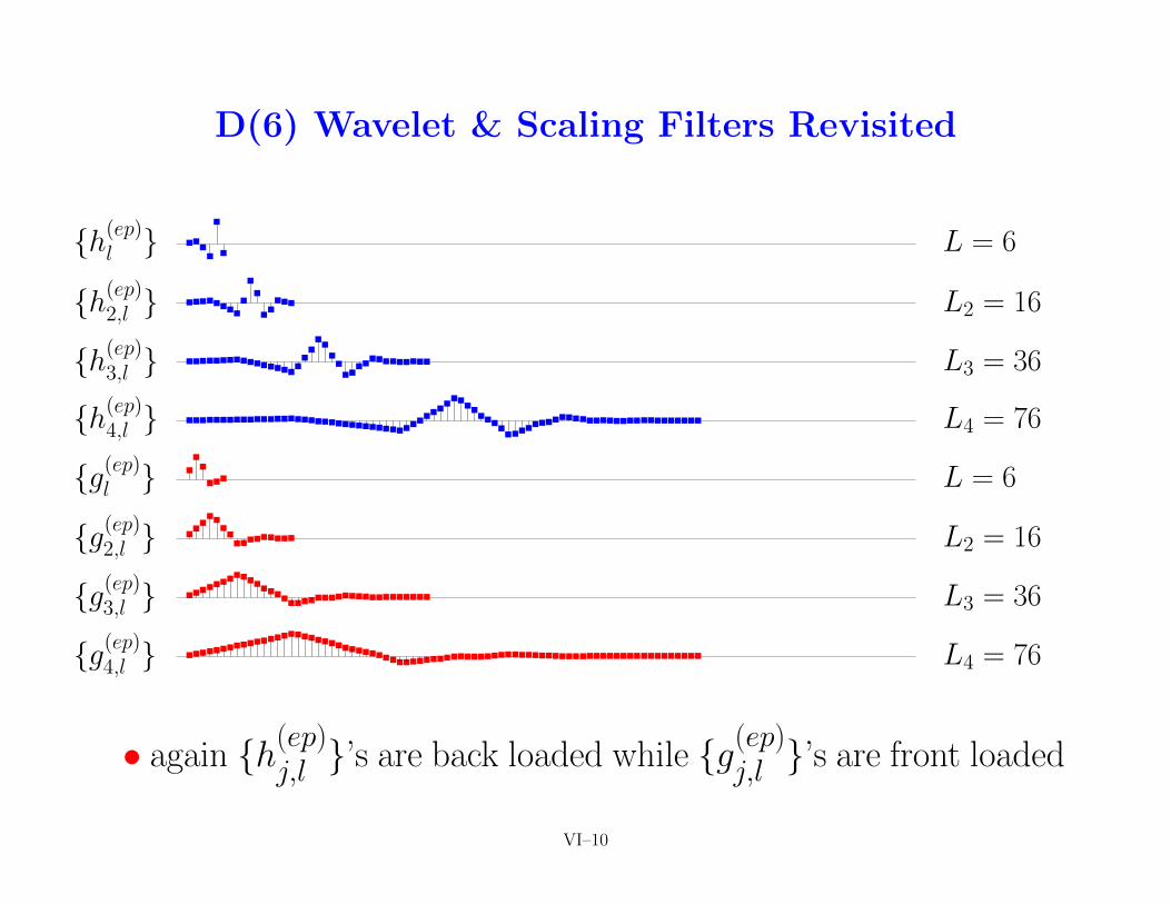
D(6) Wavelet & Scaling Filters Revisited
...
.
.
.
........
.
.
.
..
...
.................
.
.
..
.
.
.............
............................................................................
.
.
.
...
.....
..
.........
....................................
....................................
........................................
{h(ep)l }
{h(ep)2,l }
{h(ep)3,l }
{h(ep)4,l }
{g(ep)l }
{g(ep)2,l }
{g(ep)3,l }
{g(ep)4,l }
L = 6
L2 = 16
L3 = 36
L4 = 76
L = 6
L2 = 16
L3 = 36
L4 = 76
• again {h(ep)j,l }’s are back loaded while {g(ep)
j,l }’s are front loaded
VI–10
Least Asymmetric Scaling Filters: Introduction
• denote these filters by {g(la)l }
• idea is to pick the filter closest to being symmetric, with sym-metry being measured in terms of the phase function θ(·):
G(D)(f ) =
√G(D)(f )eiθ(f )
• filter of width L called LA(L) scaling filter; e.g., LA(8), LA(16)
• LA(2), LA(4) and LA(6) same as Haar, D(4) and D(6)
• LA(L) and D(L) scaling filters differ for L = 8, 10, 12, . . .
• Q: why is symmetry of interest?
WMTSA: 107–108 VI–11
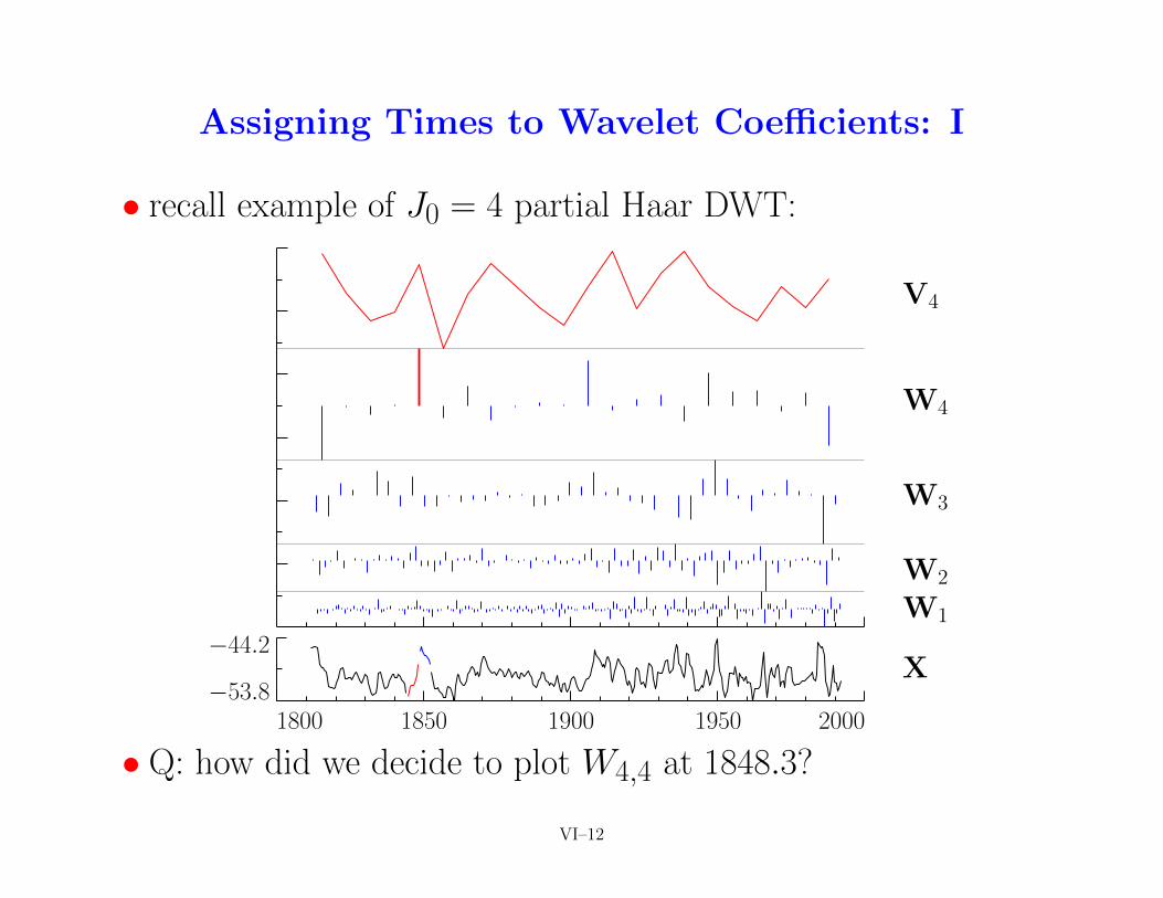
Assigning Times to Wavelet Coefficients: I
• recall example of J0 = 4 partial Haar DWT:
V4
W4
W3
W2
W1
X−44.2
−53.81800 1850 1900 1950 2000
• Q: how did we decide to plot W4,4 at 1848.3?
VI–12
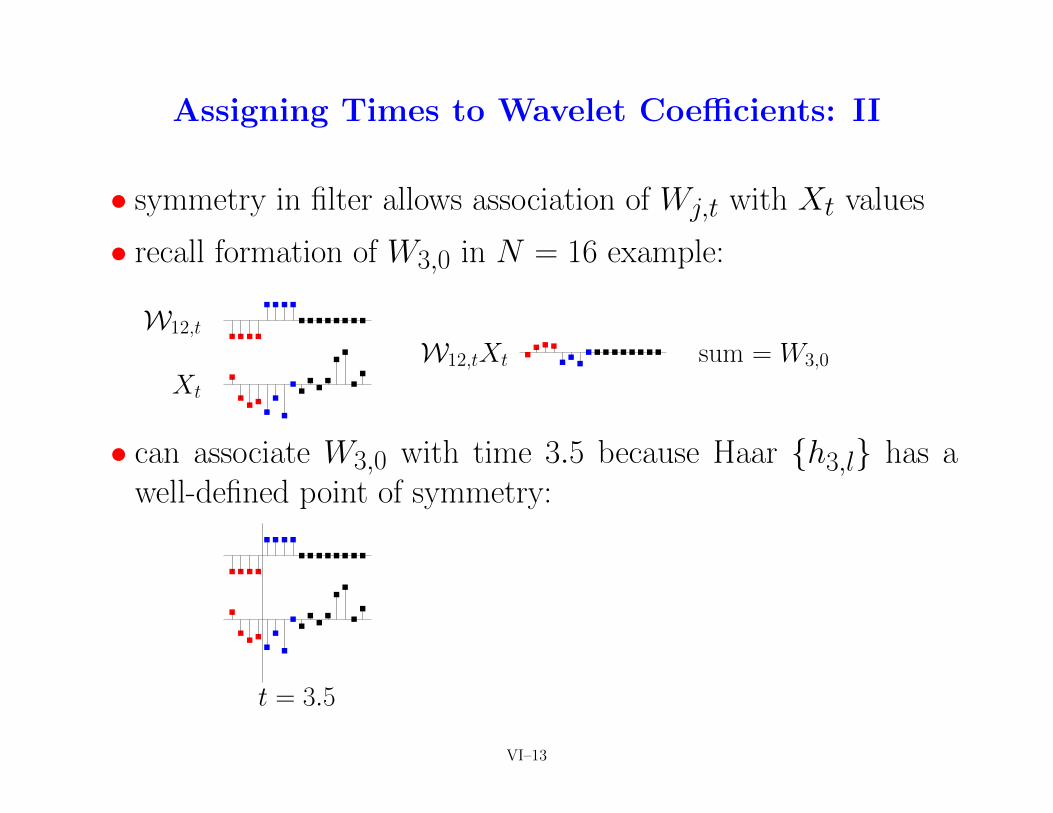
Assigning Times to Wavelet Coefficients: II
• symmetry in filter allows association of Wj,t with Xt values
• recall formation of W3,0 in N = 16 example:
....
....
........
.
.
..
.
.
.
.
.
.
.
.
.
.
.
.
.
...
...
.........
W12,t
Xt
W12,tXt sum = W3,0
• can associate W3,0 with time 3.5 because Haar {h3,l} has awell-defined point of symmetry:
....
....
........
.
.
..
.
.
.
.
.
.
.
.
.
.
.
.
t = 3.5
VI–13
Zero Phase Filters: I
• LA class of wavelet and scaling filters designed to exhibit ‘nearsymmetry’ about some point in the filter
• makes it easier to align Wj,t and VJ0,t with values in X
• can quantify symmetry by considering ‘zero phase’ filters, soneed to introduce ideas behind this type of filter
• consider filter {ul} ←→ U(·); i.e, U(f ) =∑∞l=−∞ ule
−i2πfl
• write U(f ) = |U(f )|eiθ(f ), where the gain function is definedby |U(f )|, and θ(·) is the phase function
WMTSA: 108–110 VI–14
Zero Phase Filters: II
• let {u◦l } be {ul} periodized to length N
• Exer. [33] says that {u◦l } ←→ {U( kN )}, where both l and ktake the values 0, 1, . . . , N − 1
• let {Xt} be time series of length N with DFT {Xk}• let {Yt} be {Xt} circularly filtered with {u◦l }:
Yt ≡N−1∑l=0
u◦lXt−l mod N , t = 0, 1, . . . , N − 1
• hence {Yt} ←→ {U( kN )Xk}
WMTSA: 108–110 VI–15
Zero Phase Filters: III
• since {Yt} ←→ {U( kN )Xk}, inverse DFT says
Yt =1
N
N−1∑k=0
U( kN )Xkei2πkt/N
• suppose {ul} has zero phase; i.e., θ(f ) = 0 for all f
• since U(f ) = |U(f )|, have U( kN ) = |U( kN )|, so
Yt =1
N
N−1∑k=0
|U( kN )|Xkei2πkt/N
• |U( kN )|Xk & Xk have the same phase, but amplitudes can differ
• thus components in output {Yt} that are undamped by filterwill line up with similar components in input {Xt}
WMTSA: 108–110 VI–16
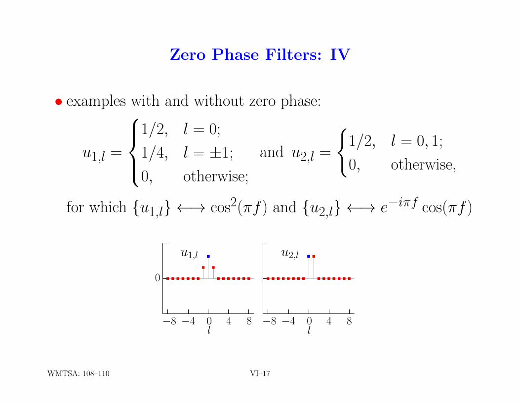
Zero Phase Filters: IV
• examples with and without zero phase:
u1,l =
1/2, l = 0;
1/4, l = ±1;
0, otherwise;
and u2,l =
{1/2, l = 0, 1;
0, otherwise,
for which {u1,l} ←→ cos2(πf ) and {u2,l} ←→ e−iπf cos(πf )
.......
.
.
.
....... ........
..
.......
. .u1,l u2,l
0
−8 −4 0 4 8 −8 −4 0 4 8l l
WMTSA: 108–110 VI–17
Zero Phase Filters: V
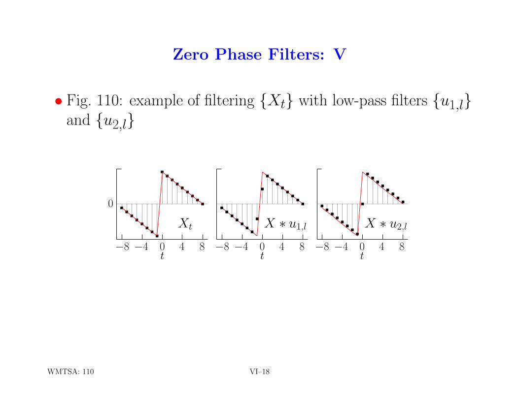
• Fig. 110: example of filtering {Xt} with low-pass filters {u1,l}and {u2,l}
.
.
.
.
.
.
.
.
.
.
.
.
.
.
.
.
.
.
.
.
.
.
.
.
.
.
.
.
.
.
.
.
.
..
.
.
.
.
.
.
.
.
.
.
.
.
.
.
.
.
Xt X ∗ u1,l X ∗ u2,l0
−8 −4 0 4 8 −8 −4 0 4 8 −8 −4 0 4 8t t t
WMTSA: 110 VI–18
Linear Phase Filters: I
• LA {gl}’s formulated in terms of linear phase filters
• to relate linear phase and zero phase ideas, consider circularlyshifting {Yt} by ν units:
Y(ν)t ≡ Yt+ν mod N , t = 0, . . . , N − 1
• example: ν = 2 & N = 11 yields Y(2)
8 = Y8+2 mod 11 = Y10,
with Y(2)
8 occurring 2 time units earlier than Y10
• {Y (ν)t } advanced version of {Yt} if ν > 0
• {Y (ν)t } delayed version of {Yt} if ν < 0
WMTSA: 111 VI–19

Linear Phase Filters: II
• note following:
Y(ν)t = Yt+ν mod N =
N−1∑l=0
u◦lXt+ν−l mod N
=
N−1−ν∑l=−ν
u◦l+νXt−l mod N
=
N−1−ν∑l=−ν
u◦l+ν mod NXt−l mod N
=
N−1∑l=0
u◦l+ν mod NXt−l mod N
• thus can advance filter output by advancing filter
WMTSA: 111 VI–20
Linear Phase Filters: III
• {u◦l+ν mod N : l = 0, . . . , N − 1} periodized version of
{u(ν)l ≡ ul+ν : l = . . . ,−1, 0, 1, . . .}
• phase properties of {u◦l+ν mod N} depend on transfer function
U (ν)(·) for {u(ν)l }
• Exer. [111]: U (ν)(f ) = ei2πfνU(f )
• suppose {ul} has zero phase so U(f ) = |U(f )|
• implies {u(ν)l } has θ(ν)(f ) = 2πfν
• {u(ν)l } said to have linear phase
• conclusion: if ν is an integer, can convert linear phase filter tozero phase filter by appropriately advancing the filter
WMTSA: 111 VI–21
Linear Phase Filters: IV
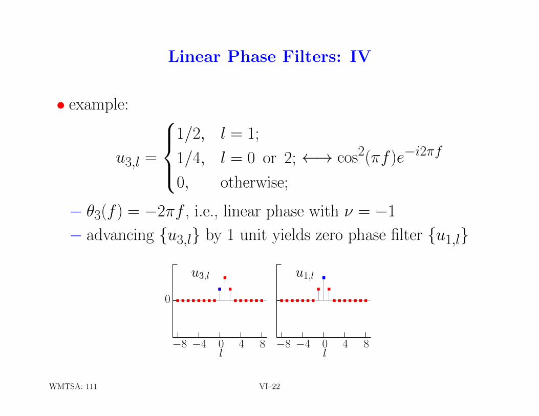
• example:
u3,l =
1/2, l = 1;
1/4, l = 0 or 2;
0, otherwise;
←→ cos2(πf )e−i2πf
− θ3(f ) = −2πf , i.e., linear phase with ν = −1
− advancing {u3,l} by 1 unit yields zero phase filter {u1,l}
.......
.
.
.
...............
.
.
.
......
.
.
u3,l u1,l
0
−8 −4 0 4 8 −8 −4 0 4 8l l
WMTSA: 111 VI–22
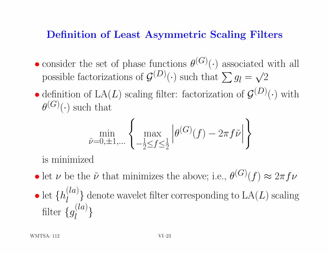
Definition of Least Asymmetric Scaling Filters
• consider the set of phase functions θ(G)(·) associated with all
possible factorizations of G(D)(·) such that∑gl =
√2
• definition of LA(L) scaling filter: factorization of G(D)(·) with
θ(G)(·) such that
minν=0,±1,...
{max−1
2≤f≤12
∣∣∣θ(G)(f )− 2πfν∣∣∣}
is minimized
• let ν be the ν that minimizes the above; i.e., θ(G)(f ) ≈ 2πfν
• let {h(la)l } denote wavelet filter corresponding to LA(L) scaling
filter {g(la)l }
WMTSA: 112 VI–23
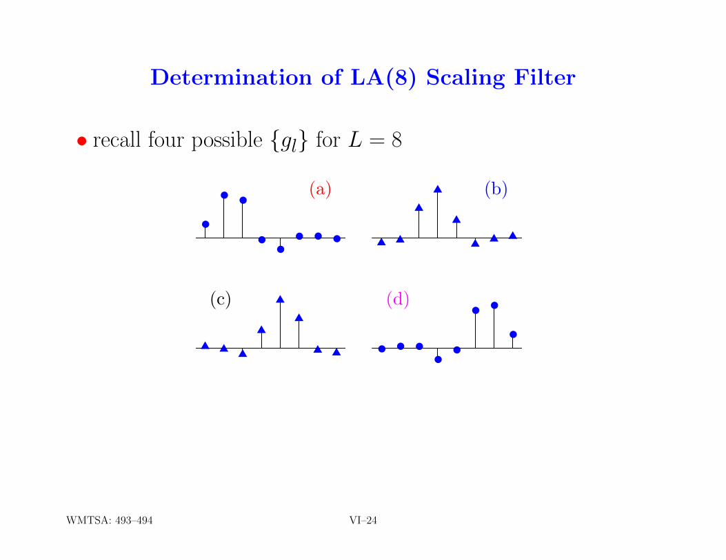
Determination of LA(8) Scaling Filter
• recall four possible {gl} for L = 8
●
●●
●●
● ● ●
(a) (b)
(c)
● ● ●
●●
●●
●
(d)
WMTSA: 493–494 VI–24
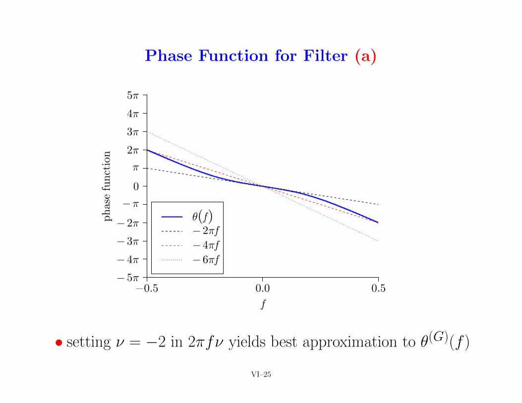
Phase Function for Filter (a)
−0.5 0.0 0.5− 5π
− 4π
− 3π
− 2π
−π
0
π
2π
3π
4π
5π
f
phas
e fu
ncti
on
θ(f)−2πf−4πf−6πf
• setting ν = −2 in 2πfν yields best approximation to θ(G)(f )
VI–25
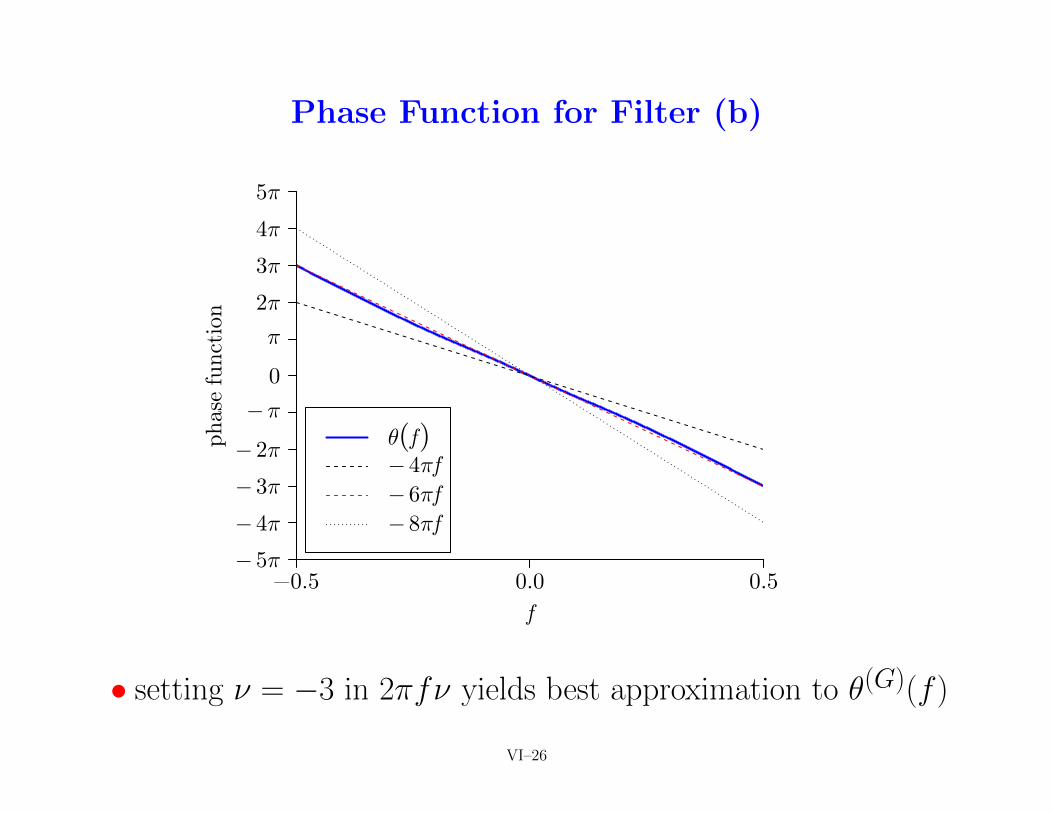
Phase Function for Filter (b)
−0.5 0.0 0.5− 5π
− 4π
− 3π
− 2π
−π
0
π
2π
3π
4π
5π
f
phas
e fu
ncti
on
θ(f)−4πf−6πf−8πf
• setting ν = −3 in 2πfν yields best approximation to θ(G)(f )
VI–26
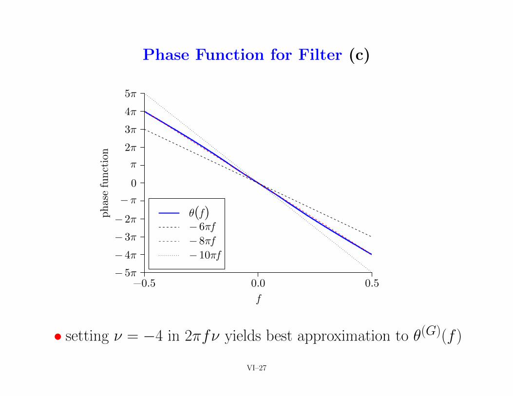
Phase Function for Filter (c)
−0.5 0.0 0.5− 5π
− 4π
− 3π
− 2π
−π
0
π
2π
3π
4π
5π
f
phas
e fu
ncti
on
θ(f)−6πf−8πf−10πf
• setting ν = −4 in 2πfν yields best approximation to θ(G)(f )
VI–27
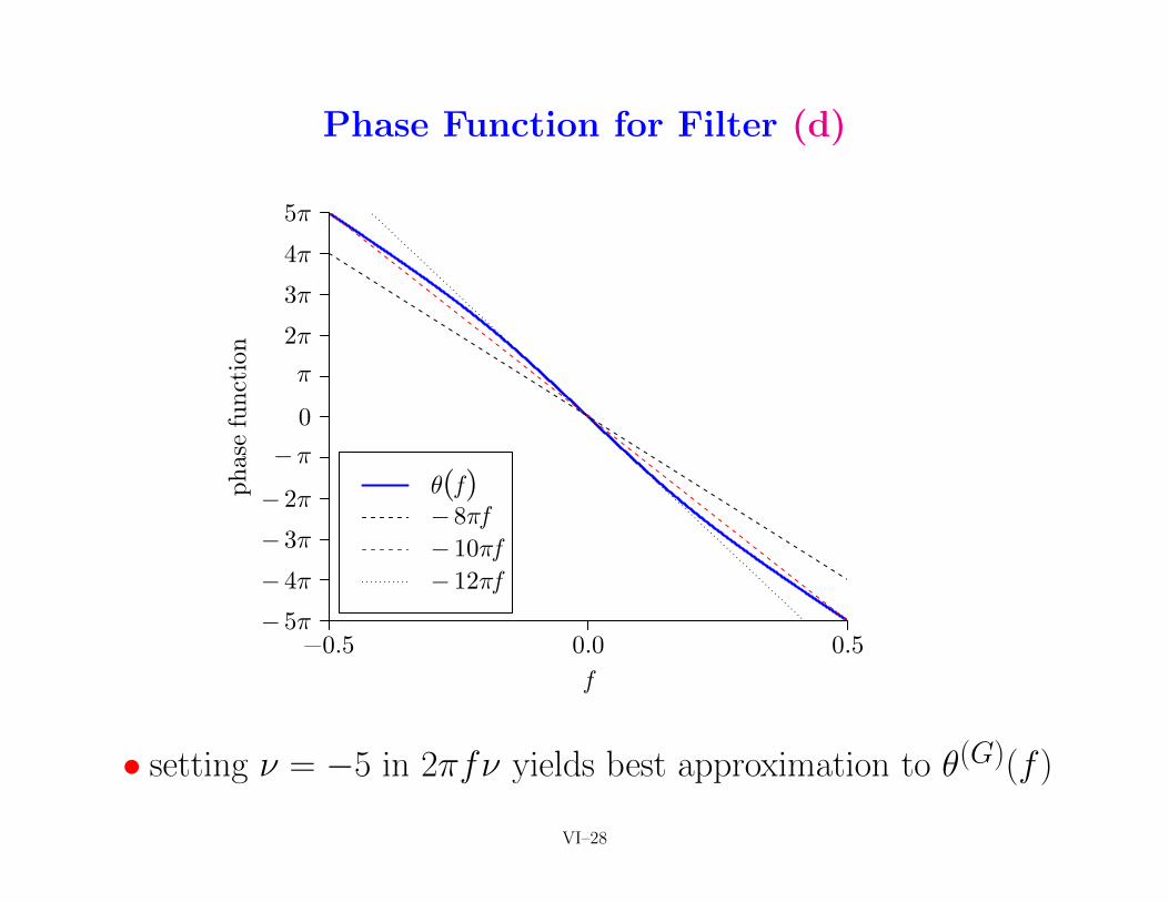
Phase Function for Filter (d)
−0.5 0.0 0.5− 5π
− 4π
− 3π
− 2π
−π
0
π
2π
3π
4π
5π
f
phas
e fu
ncti
on
θ(f)−8πf−10πf−12πf
• setting ν = −5 in 2πfν yields best approximation to θ(G)(f )
VI–28
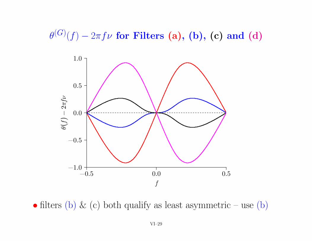
θ(G)(f )− 2πfν for Filters (a), (b), (c) and (d)
−0.5 0.0 0.5−1.0
−0.5
0.0
0.5
1.0
f
θ(f)
−2π
fν
• filters (b) & (c) both qualify as least asymmetric – use (b)
VI–29
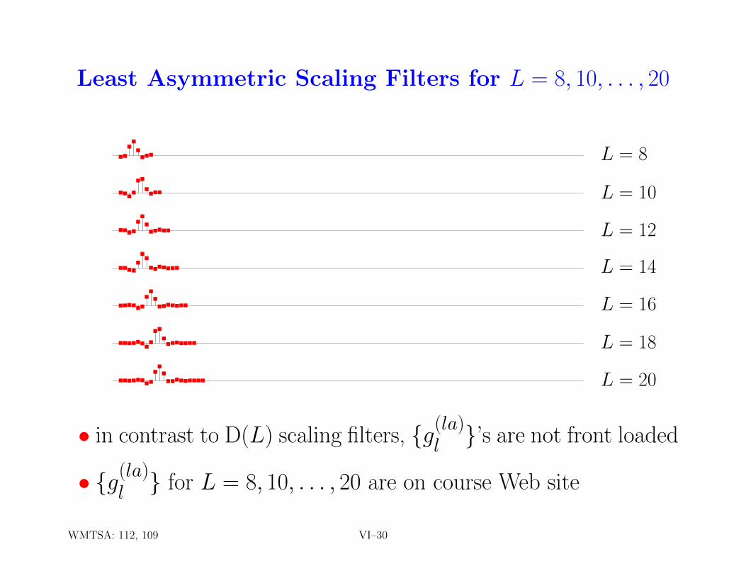
Least Asymmetric Scaling Filters for L = 8, 10, . . . , 20
..
.
.
.
...
....
..
....
....
.
.
.
.....
....
.
..
.......
......
.
.
.
.......
........
..
.
.......
........
.
.
.
.........
L = 8
L = 10
L = 12
L = 14
L = 16
L = 18
L = 20
• in contrast to D(L) scaling filters, {g(la)l }’s are not front loaded
• {g(la)l } for L = 8, 10, . . . , 20 are on course Web site
WMTSA: 112, 109 VI–30
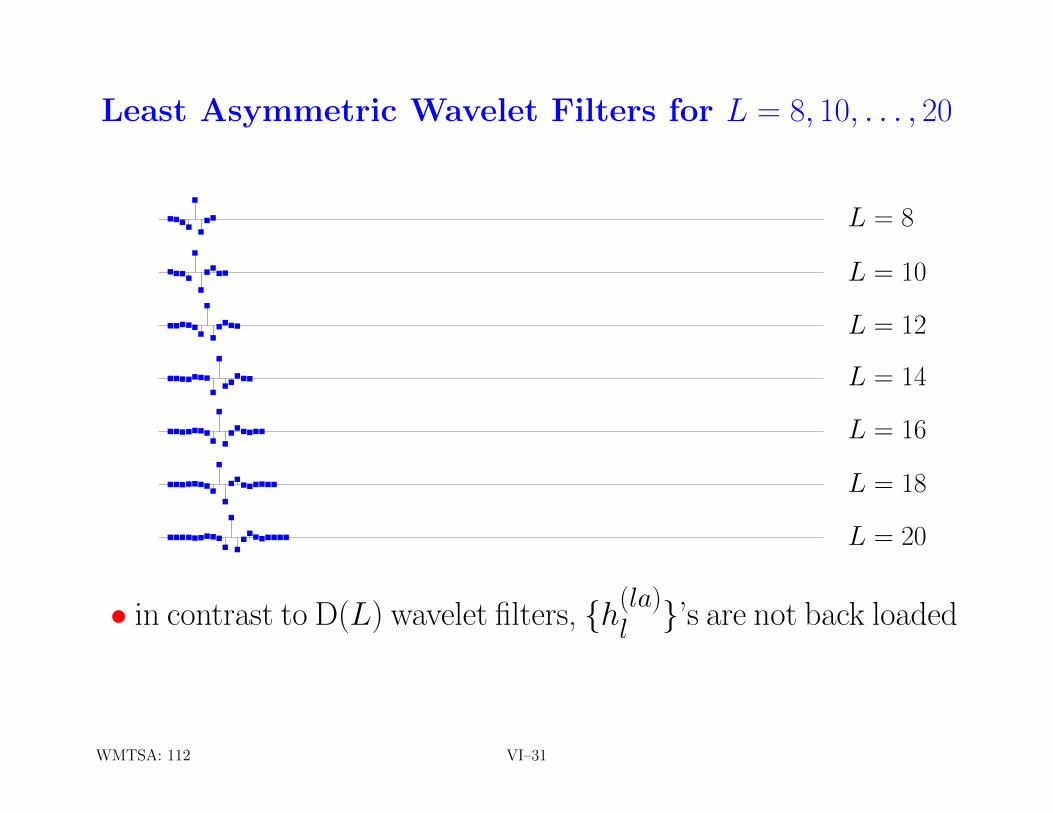
Least Asymmetric Wavelet Filters for L = 8, 10, . . . , 20
....
.
.
..
....
.
.
....
......
.
.
....
.......
.
.
.....
.......
.
.
.
......
........
.
.
........
.........
.
.
.
........
L = 8
L = 10
L = 12
L = 14
L = 16
L = 18
L = 20
• in contrast to D(L) wavelet filters, {h(la)l }’s are not back loaded
WMTSA: 112 VI–31
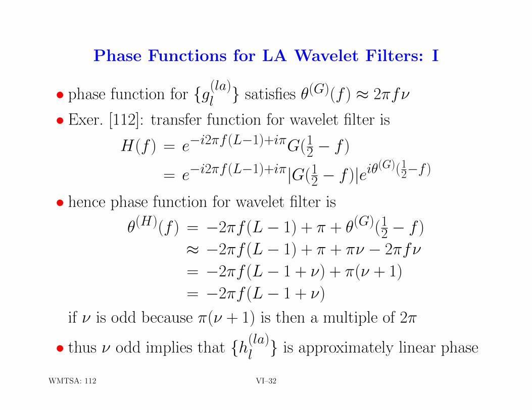
Phase Functions for LA Wavelet Filters: I
• phase function for {g(la)l } satisfies θ(G)(f ) ≈ 2πfν
• Exer. [112]: transfer function for wavelet filter is
H(f ) = e−i2πf (L−1)+iπG(12 − f )
= e−i2πf (L−1)+iπ|G(12 − f )|eiθ
(G)(12−f )
• hence phase function for wavelet filter is
θ(H)(f ) = −2πf (L− 1) + π + θ(G)(12 − f )
≈ −2πf (L− 1) + π + πν − 2πfν
= −2πf (L− 1 + ν) + π(ν + 1)
= −2πf (L− 1 + ν)
if ν is odd because π(ν + 1) is then a multiple of 2π
• thus ν odd implies that {h(la)l } is approximately linear phase
WMTSA: 112 VI–32

Phase Functions for LA Wavelet Filters: II
• for tabulated LA coefficients, have
ν =
−L2 + 1, if L = 8, 12, 16, 20 (i.e., L2 is even);
−L2 , if L = 10 or 18;
−L2 + 2, if L = 14,
so ν is indeed odd for all 7 LA scaling filters
• conclusion: LA wavelet filters also ≈ linear phase
• appropriate shift to get zero phase is −(L− 1 + ν)
WMTSA: 112–113 VI–33
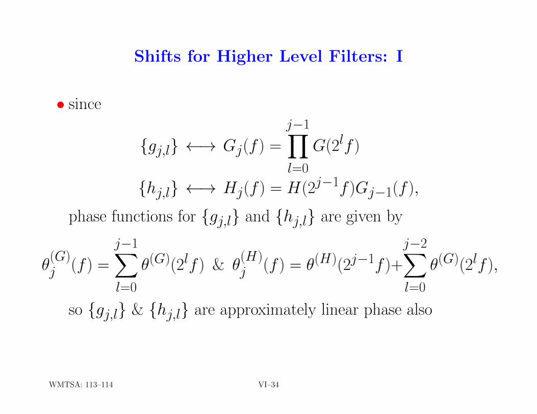
Shifts for Higher Level Filters: I
• since
{gj,l} ←→ Gj(f ) =
j−1∏l=0
G(2lf )
{hj,l} ←→ Hj(f ) = H(2j−1f )Gj−1(f ),
phase functions for {gj,l} and {hj,l} are given by
θ(G)j (f ) =
j−1∑l=0
θ(G)(2lf ) & θ(H)j (f ) = θ(H)(2j−1f )+
j−2∑l=0
θ(G)(2lf ),
so {gj,l} & {hj,l} are approximately linear phase also
WMTSA: 113–114 VI–34
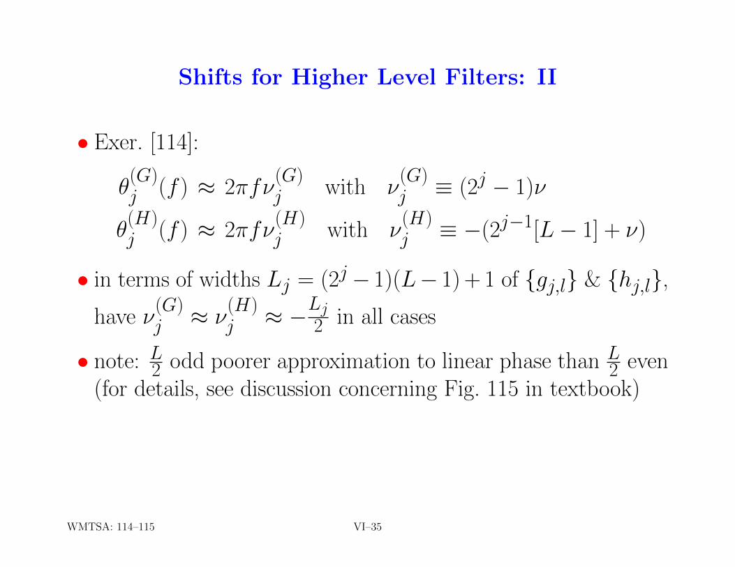
Shifts for Higher Level Filters: II
• Exer. [114]:
θ(G)j (f ) ≈ 2πfν
(G)j with ν
(G)j ≡ (2j − 1)ν
θ(H)j (f ) ≈ 2πfν
(H)j with ν
(H)j ≡ −(2j−1[L− 1] + ν)
• in terms of widths Lj = (2j− 1)(L− 1) + 1 of {gj,l} & {hj,l},have ν
(G)j ≈ ν
(H)j ≈ −Lj2 in all cases
• note: L2 odd poorer approximation to linear phase than L2 even
(for details, see discussion concerning Fig. 115 in textbook)
WMTSA: 114–115 VI–35

Aligning Filter Outputs
• can use ν(H)j & ν
(G)J0
to align elements of Wj & VJ0with X
• working through some details (see pp. 114–5 of text), find that,if Xt is associated with actual time t0 + t∆t, LA wavelet coef-ficient Wj,t can be associated with an interval of width 2τj ∆tcentered at
t0 + (2j(t + 1)− 1− |ν(H)j | mod N) ∆t,
where, e.g., |ν(H)j | = [7(2j − 1) + 1]/2 for LA(8) wavelet
• similarly, LA scaling coefficient VJ0,t can be associated with aninterval of width λJ0
∆t centered at
t0 + (2J0(t + 1)− 1− |ν(G)J0| mod N) ∆t
WMTSA: 114–116 VI–36

LA(8) Wavelet & Scaling Filters Revisited
....
.
.
..
..........
.
.
.
.
........
......................
.
...
.
.
......................
..........................................................................................................
..
.
.
.
...
......
.....
...........
................................
..................
....................................................................
......................................
{hl}
{h2,l}
{h3,l}
{h4,l}
{gl}
{g2,l}
{g3,l}
{g4,l}
L = 8
L2 = 22
L3 = 50
L4 = 106
L = 8
L2 = 22
L3 = 50
L4 = 106
• vertical lines indicate point of approximate symmetry
WMTSA: 98 VI–37
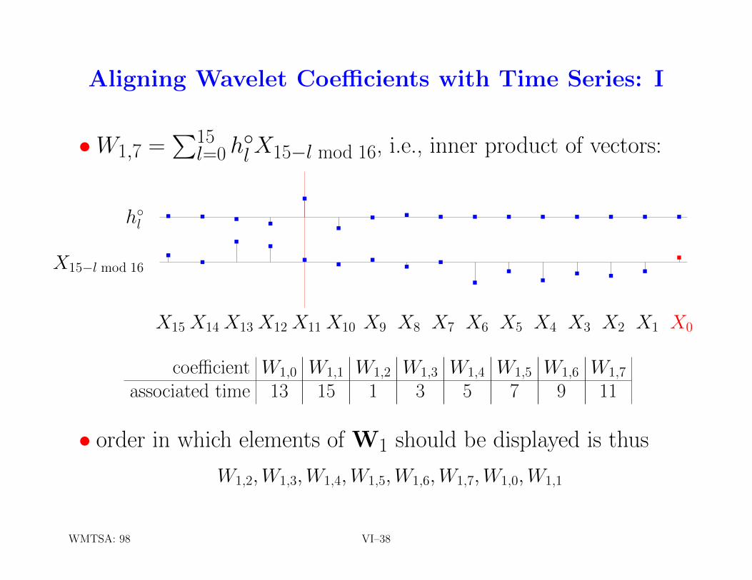
Aligning Wavelet Coefficients with Time Series: I
•W1,7 =∑15l=0 h
◦lX15−l mod 16, i.e., inner product of vectors:
. ..
.
.
.
.. . . . . . . . .
..
.
..
..
.
..
.
.
.
..
.
h◦l
X15−l mod 16
X15X14X13X12X11X10 X9 X8 X7 X6 X5 X4 X3 X2 X1 X0
coefficient W1,0 W1,1 W1,2 W1,3 W1,4 W1,5 W1,6 W1,7
associated time 13 15 1 3 5 7 9 11
• order in which elements of W1 should be displayed is thus
W1,2,W1,3,W1,4,W1,5,W1,6,W1,7,W1,0,W1,1
WMTSA: 98 VI–38
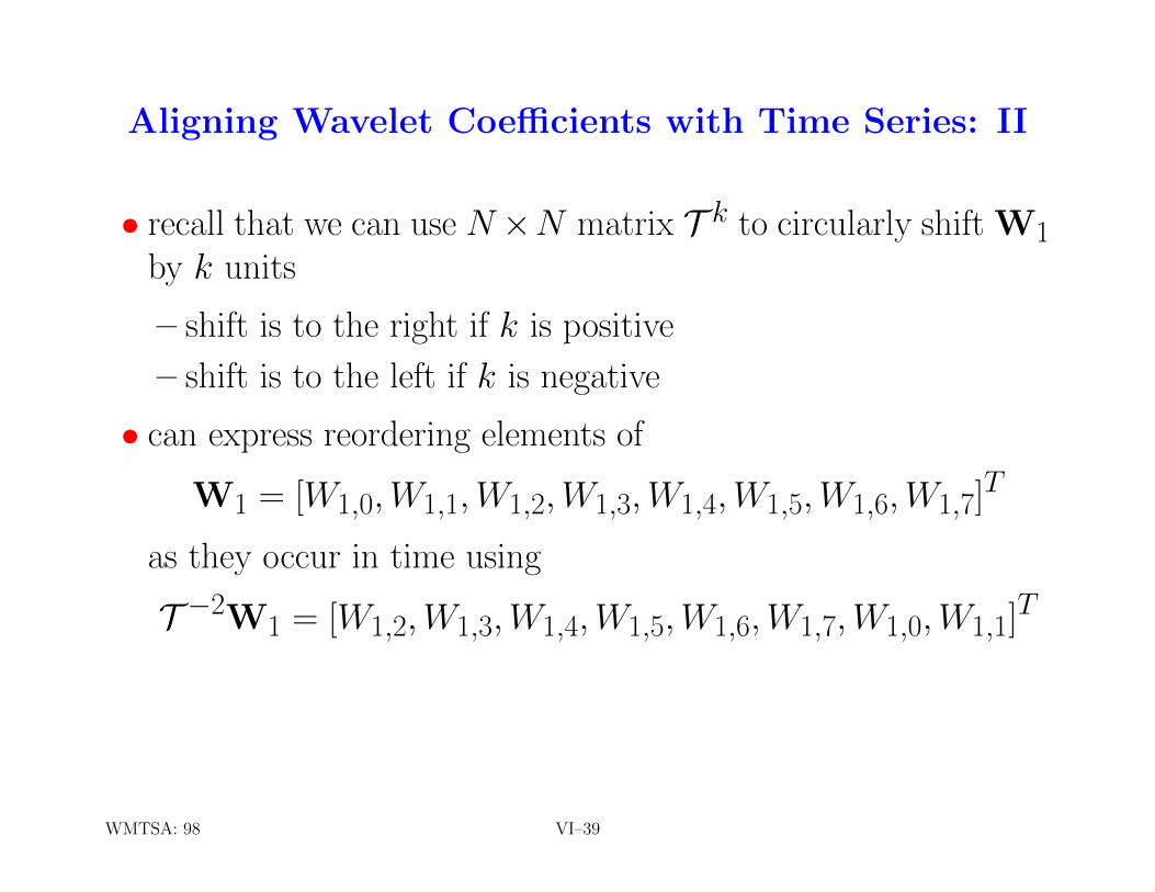
Aligning Wavelet Coefficients with Time Series: II
• recall that we can use N ×N matrix T k to circularly shift W1by k units
– shift is to the right if k is positive
– shift is to the left if k is negative
• can express reordering elements of
W1 = [W1,0,W1,1,W1,2,W1,3,W1,4,W1,5,W1,6,W1,7]T
as they occur in time using
T −2W1 = [W1,2,W1,3,W1,4,W1,5,W1,6,W1,7,W1,0,W1,1]T
WMTSA: 98 VI–39
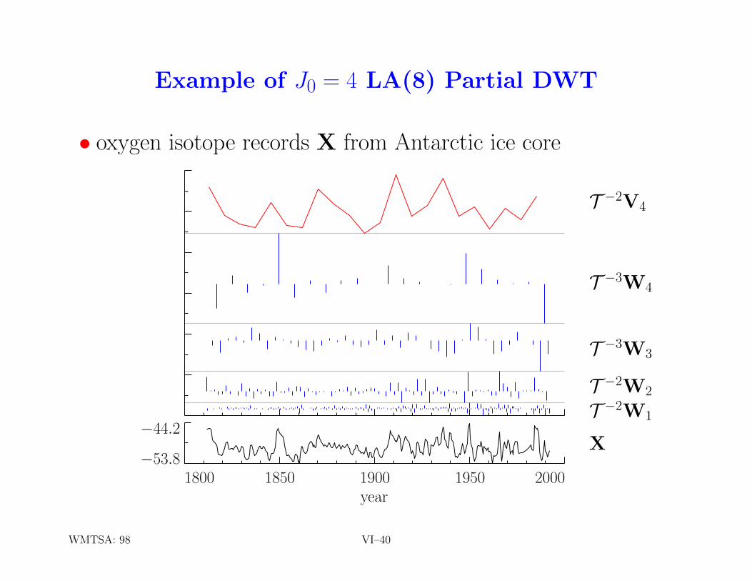
Example of J0 = 4 LA(8) Partial DWT
• oxygen isotope records X from Antarctic ice core
T −2V4
T −3W4
T −3W3
T −2W2
T −2W1
X−44.2
−53.81800 1850 1900 1950 2000
year
WMTSA: 98 VI–40
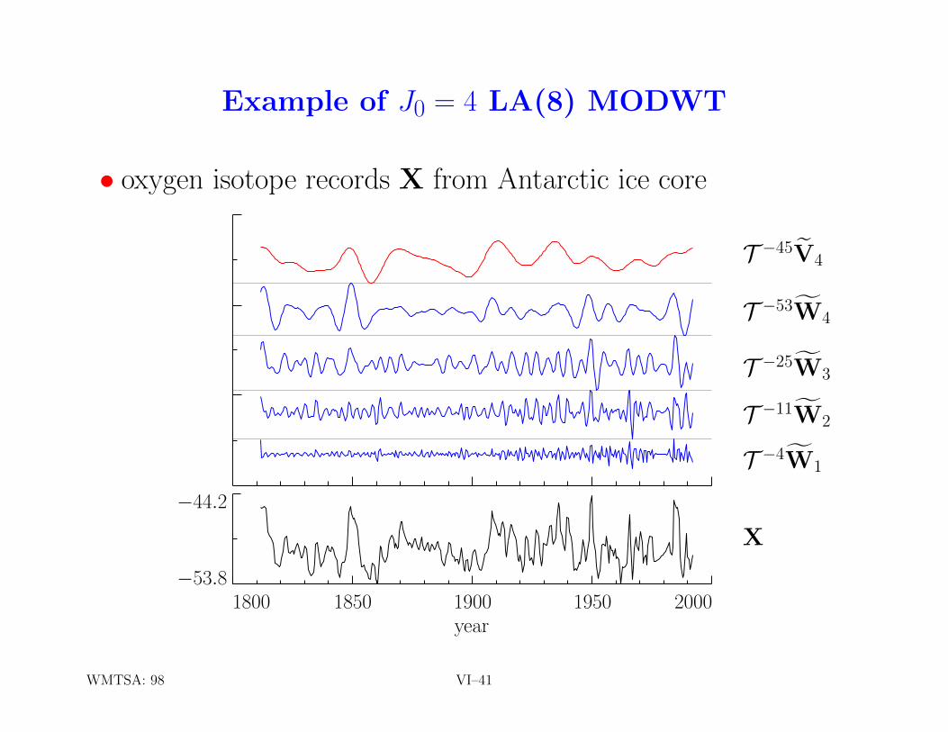
Example of J0 = 4 LA(8) MODWT
• oxygen isotope records X from Antarctic ice core
T −45V4
T −53W4
T −25W3
T −11W2
T −4W1
X
−44.2
−53.81800 1850 1900 1950 2000
year
WMTSA: 98 VI–41
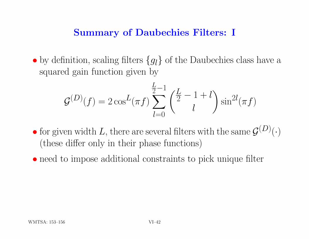
Summary of Daubechies Filters: I
• by definition, scaling filters {gl} of the Daubechies class have asquared gain function given by
G(D)(f ) = 2 cosL(πf )
L2−1∑l=0
(L2 − 1 + l
l
)sin2l(πf )
• for given width L, there are several filters with the same G(D)(·)(these differ only in their phase functions)
• need to impose additional constraints to pick unique filter
WMTSA: 153–156 VI–42
Summary of Daubechies Filters: II
• extremal (or minimum) phase constraint leads to the D(L) scal-
ing filters, denoted as {g(ep)l } (these maximize the increase in
the partial energy sequence)
• least asymmetric constraint leads to the LA(L) scaling filters,
denoted as {g(la)l }
− approximately zero phase after shifting by ν
− zero phase helps align filter output with input
− shift ν depends on L in a simple manner
− corresponding wavelet filters {h(la)l } are also approximately
zero phase after shifting by ν(H)1 ≡ −(L− 1− ν)
WMTSA: 153–156 VI–43
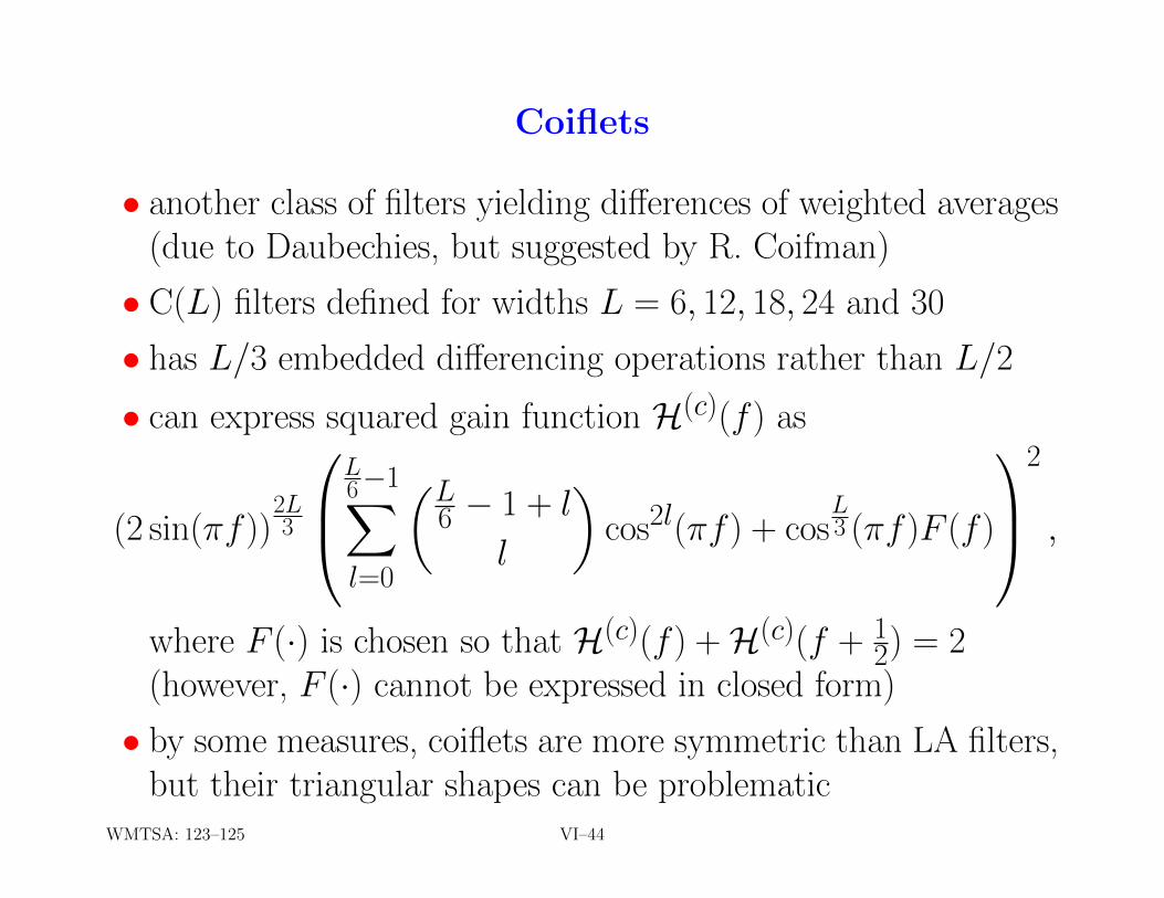
Coiflets
• another class of filters yielding differences of weighted averages(due to Daubechies, but suggested by R. Coifman)
• C(L) filters defined for widths L = 6, 12, 18, 24 and 30
• has L/3 embedded differencing operations rather than L/2
• can express squared gain function H(c)(f ) as
(2 sin(πf ))2L3
L6−1∑l=0
(L6 − 1 + l
l
)cos2l(πf ) + cos
L3 (πf )F (f )
2
,
where F (·) is chosen so that H(c)(f ) +H(c)(f + 12) = 2
(however, F (·) cannot be expressed in closed form)
• by some measures, coiflets are more symmetric than LA filters,but their triangular shapes can be problematic
WMTSA: 123–125 VI–44
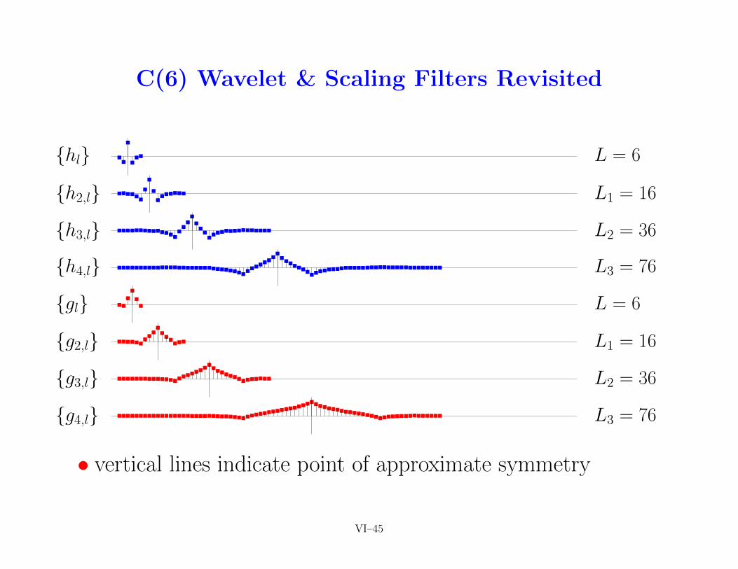
C(6) Wavelet & Scaling Filters Revisited
..
.
.
..
......
.
.
.
.......
..............
...
.
.
..
...............
............................................................................
..
.
.
.
.
..........
......
....................................
.................................................................
...........
{hl}
{h2,l}
{h3,l}
{h4,l}
{gl}
{g2,l}
{g3,l}
{g4,l}
L = 6
L1 = 16
L2 = 36
L3 = 76
L = 6
L1 = 16
L2 = 36
L3 = 76
• vertical lines indicate point of approximate symmetry
VI–45
Zero-Phase Wavelet (Zephlet) Transform: I
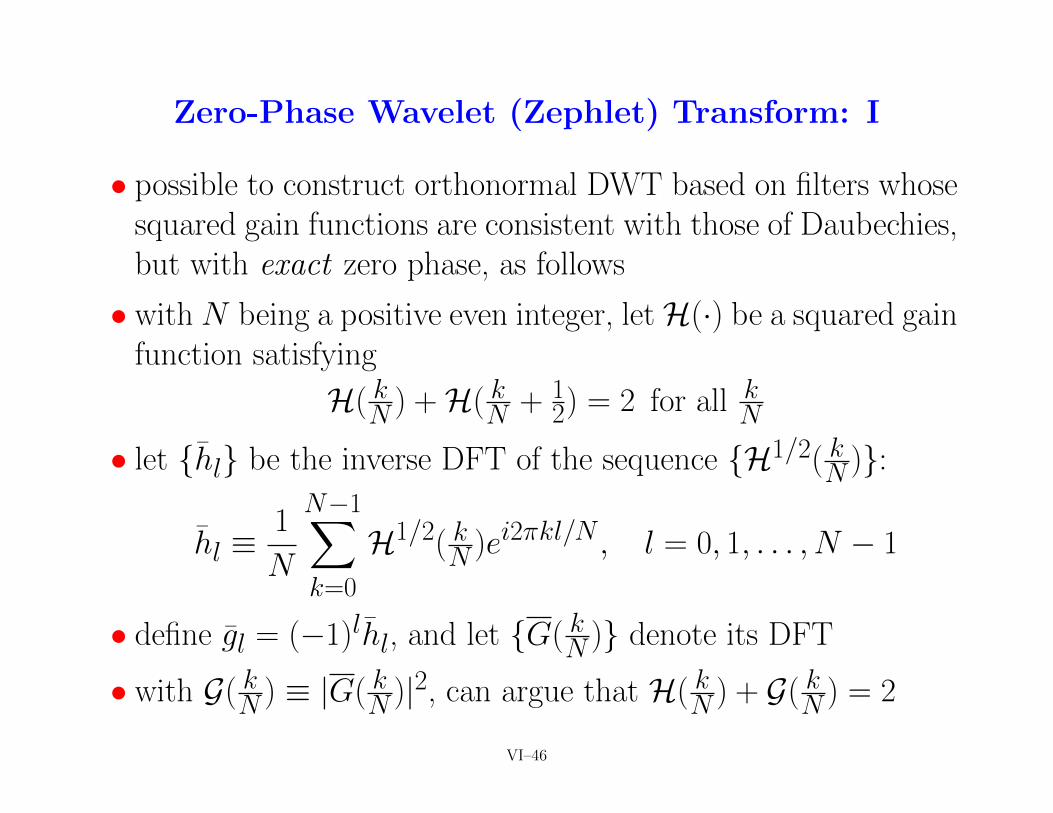
• possible to construct orthonormal DWT based on filters whosesquared gain functions are consistent with those of Daubechies,but with exact zero phase, as follows
• with N being a positive even integer, letH(·) be a squared gainfunction satisfying
H( kN ) +H( kN + 12) = 2 for all k
N
• let {hl} be the inverse DFT of the sequence {H1/2( kN )}:
hl ≡1
N
N−1∑k=0
H1/2( kN )ei2πkl/N , l = 0, 1, . . . , N − 1
• define gl = (−1)lhl, and let {G( kN )} denote its DFT
• with G( kN ) ≡ |G( kN )|2, can argue that H( kN ) + G( kN ) = 2
VI–46
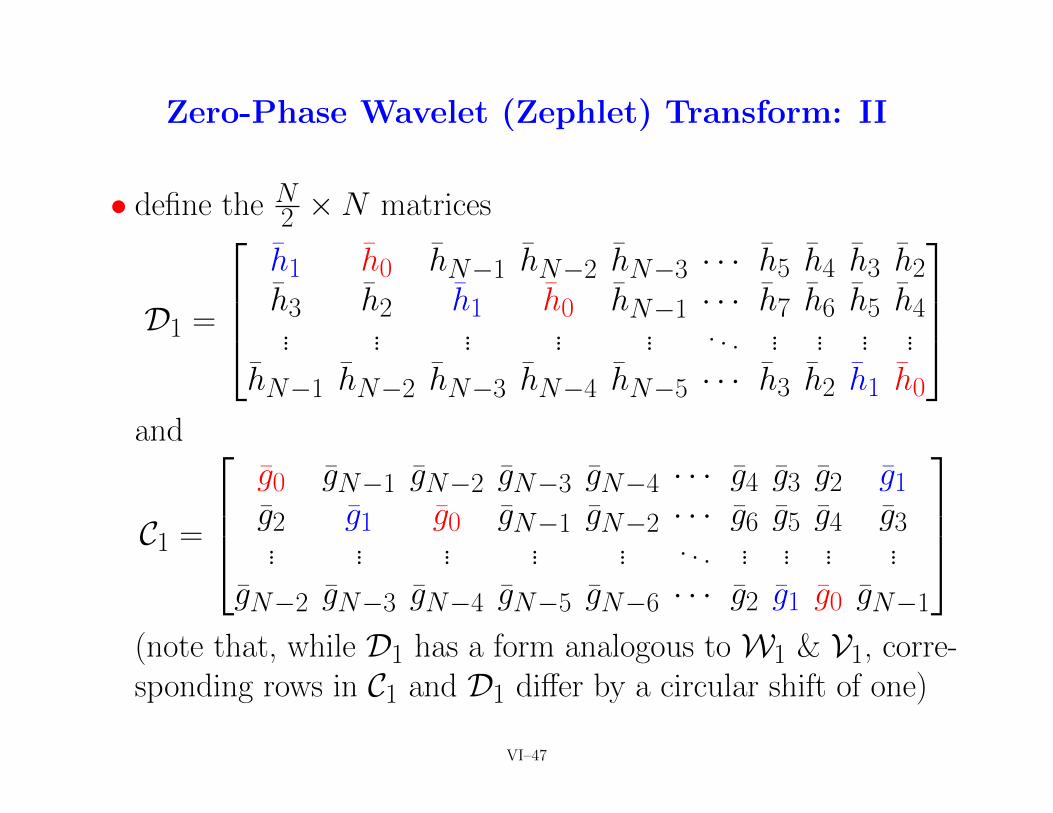
Zero-Phase Wavelet (Zephlet) Transform: II
• define the N2 ×N matrices
D1 =
h1 h0 hN−1 hN−2 hN−3 · · · h5 h4 h3 h2h3 h2 h1 h0 hN−1 · · · h7 h6 h5 h4... ... ... ... ... . . . ... ... ... ...
hN−1 hN−2 hN−3 hN−4 hN−5 · · · h3 h2 h1 h0
and
C1 =
g0 gN−1 gN−2 gN−3 gN−4 · · · g4 g3 g2 g1g2 g1 g0 gN−1 gN−2 · · · g6 g5 g4 g3... ... ... ... ... . . . ... ... ... ...
gN−2 gN−3 gN−4 gN−5 gN−6 · · · g2 g1 g0 gN−1
(note that, while D1 has a form analogous to W1 & V1, corre-sponding rows in C1 and D1 differ by a circular shift of one)
VI–47
Zero-Phase Wavelet (Zephlet) Transform: III
• can show that the N × N matrix formed by stacking D1 ontop of C1 is a real-valued orthonormal matrix; i.e,
D ≡[D1C1
]is such that DTD = IN
• proof of above result (subject of forthcoming exercise!) is similarin spirit to proof that W is orthonormal, but details differ
• algorithms for computing DWT and zephlet transform are, re-spectively, O(N) and O(N · log2(N))
VI–48
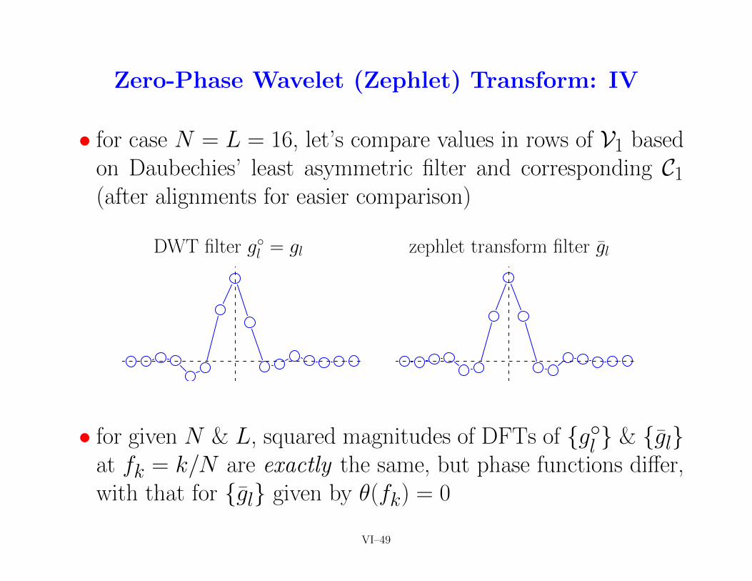
Zero-Phase Wavelet (Zephlet) Transform: IV
• for case N = L = 16, let’s compare values in rows of V1 basedon Daubechies’ least asymmetric filter and corresponding C1(after alignments for easier comparison)
DWT filter g◦l = gl zephlet transform filter gl
• for given N & L, squared magnitudes of DFTs of {g◦l } & {gl}at fk = k/N are exactly the same, but phase functions differ,with that for {gl} given by θ(fk) = 0
VI–49
Zero-Phase Wavelet (Zephlet) Transform: V
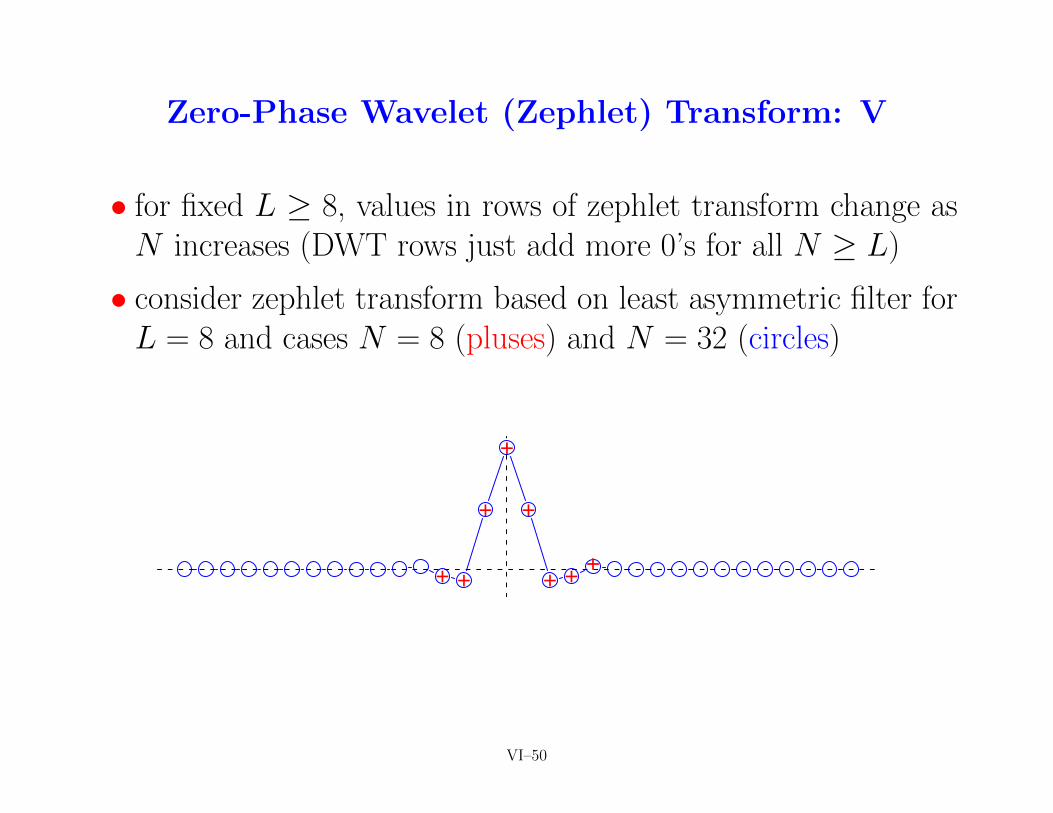
• for fixed L ≥ 8, values in rows of zephlet transform change asN increases (DWT rows just add more 0’s for all N ≥ L)
• consider zephlet transform based on least asymmetric filter forL = 8 and cases N = 8 (pluses) and N = 32 (circles)
+ +
+
+
+
+ ++
VI–50

Zero-Phase Wavelet (Zephlet) Transform: VI
• can work out expression for elements in zephlet transform ex-plicitly in Haar case (L = 2):
gl =
√2
N
[1 + (−1)lSl,+ + (−1)l+1Sl,−
]≈ 2(−1)l
√2
π(1− 4l2)for large N = 2M , where
Sl,± ≡ sin([2l ± 1]πM−14M )
sin(π2l±14 )
sin(π2l±14M )
• Haar-based {gl} for N = 32:
VI–51

Comparison of Outputs from LA(8) & ZephletScaling Filters (Input is Doppler Signal)
20 25 30 35 40
VI–52