Lab 2 Spontaneous Parametric DownConversion and State Projection

Week 2

Phys434L Quantum Mechanics Lab2021

February 20, 2021

1 The Overall Picture

As mentioned in the previous lab write-up, our laboratory setup consists of preparingphoton pairs. In this process, a pump photon of energy Ep is converted into two photonsof energy E1 and E2 such that

Ep = E1 + E2, (1)

or expressed in terms of the wavelength in vacuum via E = hc/λ,

1

λp=

1

λ1+

1

λ2, (2)

In a birefringent medium, spontaneous parametric down-conversion occurs due to the in-teraction of the light and the medium. For down-conversion to occur, momentum must beconserved:

~pp = ~p1 + ~p2. (3)

If the down-conversion photons have the same energy, then they come our at equal andopposite angles from the original direction of the parent photon. The two photons areproduced simultaneously from a parent photon. In this experiment we use this method to“herald” a photon that is subject to quantum operations. Another way to think about itis that we use one photon to “tag” the other photon. Then we detect both and measurethe detections in coincidence to make sure we are detecting only photons with a partner.It is a way so make sure we are doing an experiment with single photons.

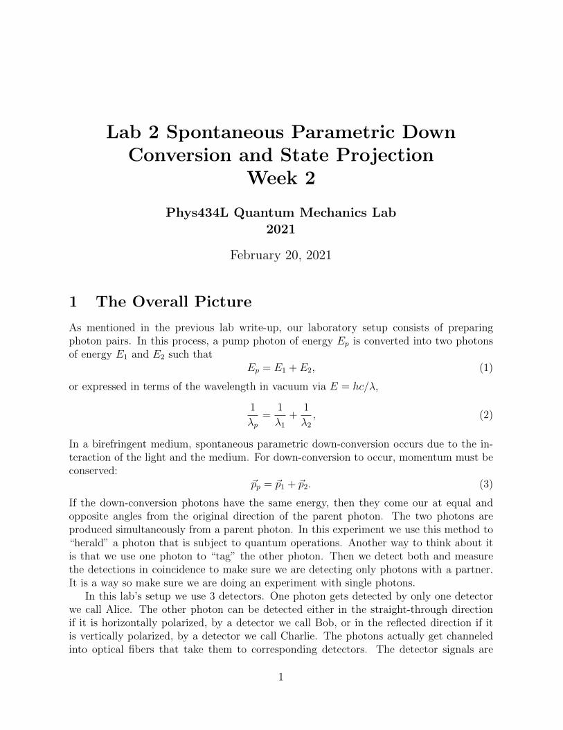
In this lab’s setup we use 3 detectors. One photon gets detected by only one detectorwe call Alice. The other photon can be detected either in the straight-through directionif it is horizontally polarized, by a detector we call Bob, or in the reflected direction if itis vertically polarized, by a detector we call Charlie. The photons actually get channeledinto optical fibers that take them to corresponding detectors. The detector signals are

1

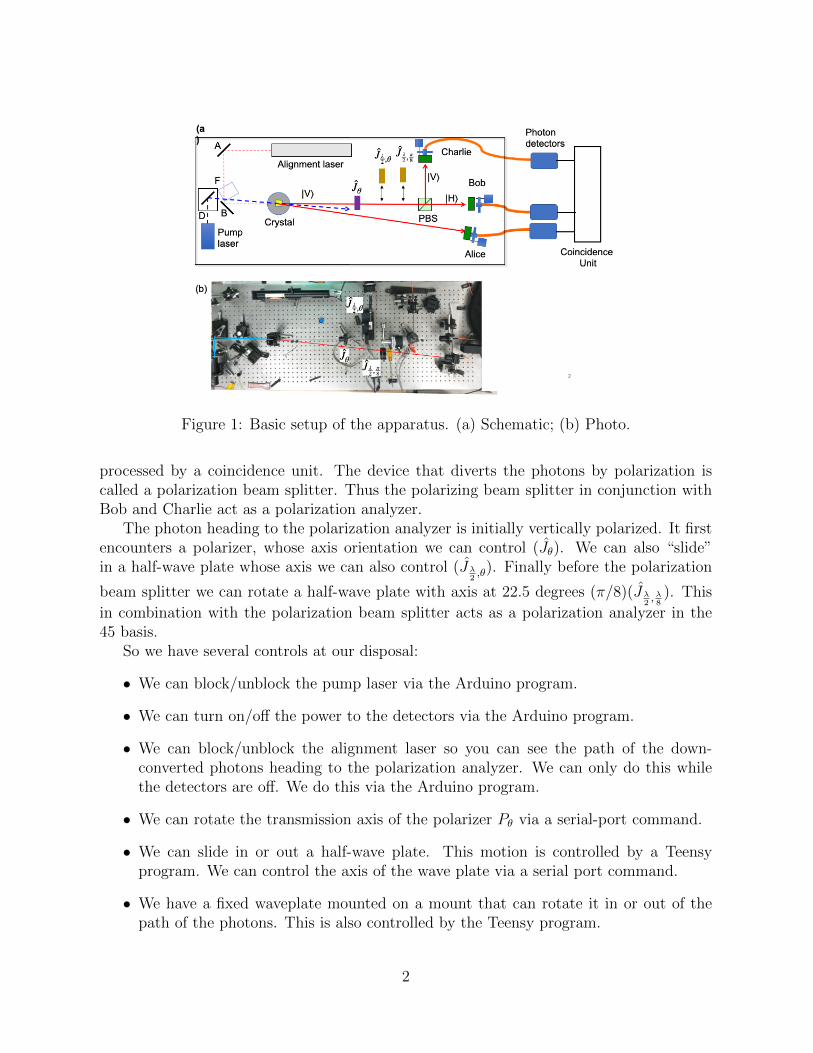
Figure 1: Basic setup of the apparatus. (a) Schematic; (b) Photo.

processed by a coincidence unit. The device that diverts the photons by polarization iscalled a polarization beam splitter. Thus the polarizing beam splitter in conjunction withBob and Charlie act as a polarization analyzer.

The photon heading to the polarization analyzer is initially vertically polarized. It firstencounters a polarizer, whose axis orientation we can control (Jθ). We can also “slide”in a half-wave plate whose axis we can also control (Jλ

2,θ). Finally before the polarization

beam splitter we can rotate a half-wave plate with axis at 22.5 degrees (π/8)(Jλ2,λ8). This

in combination with the polarization beam splitter acts as a polarization analyzer in the45 basis.

So we have several controls at our disposal:

• We can block/unblock the pump laser via the Arduino program.

• We can turn on/off the power to the detectors via the Arduino program.

• We can block/unblock the alignment laser so you can see the path of the down-converted photons heading to the polarization analyzer. We can only do this whilethe detectors are off. We do this via the Arduino program.

• We can rotate the transmission axis of the polarizer Pθ via a serial-port command.

• We can slide in or out a half-wave plate. This motion is controlled by a Teensyprogram. We can control the axis of the wave plate via a serial port command.

• We have a fixed waveplate mounted on a mount that can rotate it in or out of thepath of the photons. This is also controlled by the Teensy program.

2

• We record the photons that are detected by Alice, Bob and Charlie. We can alsorecord the coincidences between Alice and Bob and between Alice and Charlie. Wedo this with a Matlab program.

2 The Remote Apparatus

2.1 General

You will log into the lab computer using remote desktop. Once you do this, your screenwill appear as something like what you see in Fig. 2. You will see 5 windows. One is a viewof the apparatus from a webcam (center in the photo). The window on the upper left is aserial interface to the Arduino based circuit that has three functions: To block/unblock the(blue) pump laser, and to turn ON/OFF the power to the detectors, and block/unblockthe (red) alignment laser (more on this below). On the lower left is a Teensy window thatcontrols the positioning of two half-wave plates, one via a linear stage and another onevia the rotation of an arm holding it. The lower two windows are serial controls for therotating elements: the polarizer and the sliding half-wave plate. On the right is a windowwith the Matlab platform that is used to record the data from the 3 detectors.

Figure 2: Screen of the Desktop that controls the experiment in the lab. It has a webcamwindow (center), an Arduino interface window (upper left), a Teensy interface (lower left)two serial interface windows (lower center) and a Matlab window (right).

3

2.2 Commands

Here we detail the commands for the different programs. All commands given below arewithin quotation marks. Do not enter the quotation marks.

2.2.1 Logging in

You log into the lab computer using remote desktop. The address of the PC is:Ho313-96143W.colgate.edu

Then you log into the PC:Username: phas2Password: Fr2=Gm1m2

2.2.2 Arduino Interface

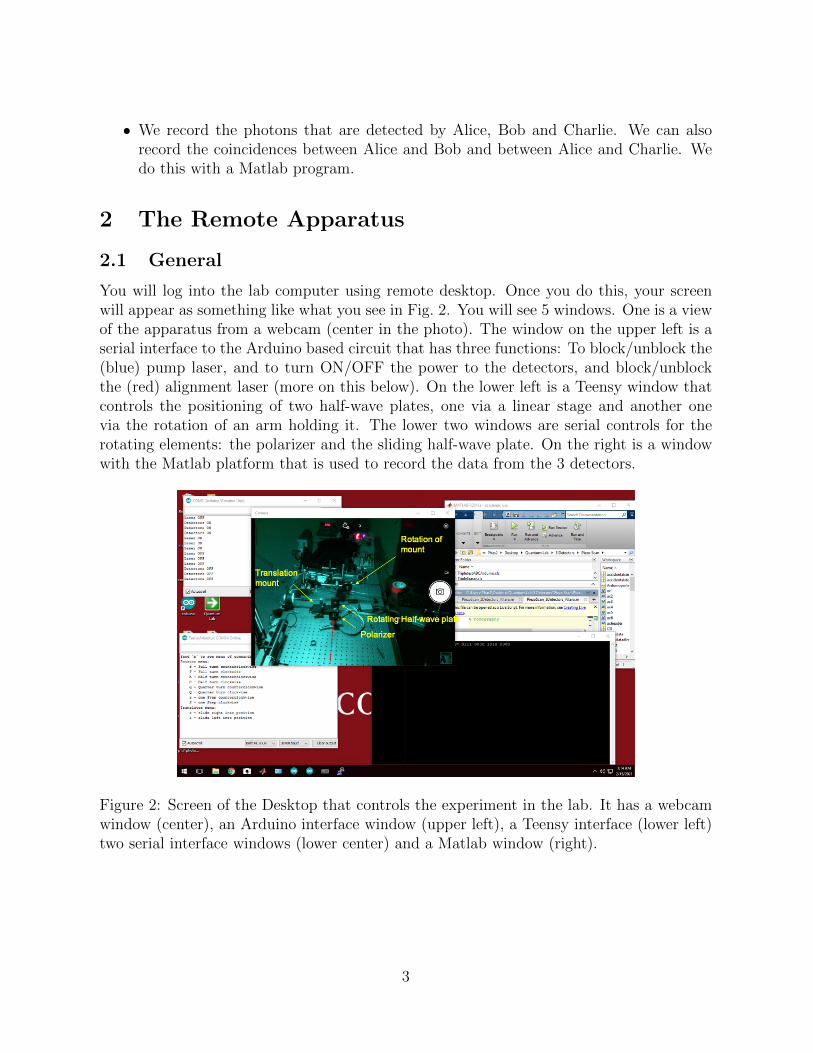
This action is for providing safety in the lab. The laser (class IV) is always on, butthat creates a safety issue, so the laser beam is blocked. Turning the laser on/off doesnot work well because there is a warm-up time for which the laser is unstable and itswavelength drifts, so the laser is left on and the beam is blocked or unblocked, as shownin Fig. 3. The laser blocker and detector power are controlled by a program that runs onan Arduino/Teensy circuit (in case you know what this is). We have this option for the3 detectors (Alice, Bob and Charlie) because they are very sensitive and so it is better toturn them off when not in use. Because we have a moving parts, we have an option fora better view of the alignments: to unblock the alignment laser. However, the detectorsmust be off when this laser is on.

Figure 3: Photo of the pump laser and beam blocker.

The Arduino program is always running. A serial window is shown in the figure. Thecommand is entered on the top command line. The action taken is listed in the lower partof the window. A summary of commands is:

• Pump Laser ON (Unblocked): On the command line type “1” . Turn it on beforeyou start the experiments. You can do two visual verification that the beam is hittingthe polarizer mount.

4

• Pump Laser OFF (Blocked): On the command line type “2” . Turn it off onceyou are done with the lab session.

• Detectors ON: On the command line type “3” . Turn it on before you start theexperiments. There is a green LED that is turned on when the detectors are connectedto the power supply. There is also a red digital readout near the top-central part of thewebcam window that indicates how much voltage is being applied to the detectors.This voltage should be close to 5 V. The value should be slightly above 5 V but neverbelow 4.5 V (otherwise the detector signals will be unstable).

• Detectors OFF: On the command line type “4” . Turn it off once you are donewith the lab session.

• Alignment Laser ON (unblocked): On the command line type “5”. Before youdo this you must be sure that the detectors are off: the digital display seenwith the webcam must read 0.000.

• Alignment laser OFF (blocked): On the command line type “6”.

• Cold Restart: In case you need to do this, in the command bar there is a roundicon for the Arduino platform. You click on this. Then you click a right arrow in theupper left that compiles the program and loads it to the circuit. You then need to goto the top menu bar, click “Tools” and then click “Serial Monitor.” This opens thescreen that you see in the figure. Resize it and put it in the lower left. You can thenminimize the Arduino platform.

2.2.3 Teensy Interface

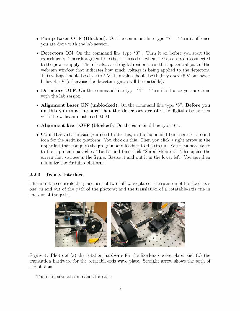
This interface controls the placement of two half-wave plates: the rotation of the fixed-axisone, in and out of the path of the photons; and the translation of a rotatable-axis one inand out of the path.

Figure 4: Photo of (a) the rotation hardware for the fixed-axis wave plate, and (b) thetranslation hardware for the rotatable-axis wave plate. Straight arrow shows the path ofthe photons.

There are several commands for each:

5

• Menu: Type “m” for a menu of the options.

• For the fixed-axis wave plate:

– “h” for half-turn counter-clockwise.

– “H” for half-turn clockwise.

– “q” quarter-turn clockwise.

– “s” one step counter-clockwise.

– “S” one step clockwise.

• For the rotatable-axis wave plate:

– “r” to slide right into path.

– “l” to slide left into path.

2.2.4 Serial Interfaces

2.2.5 Rotational Controls

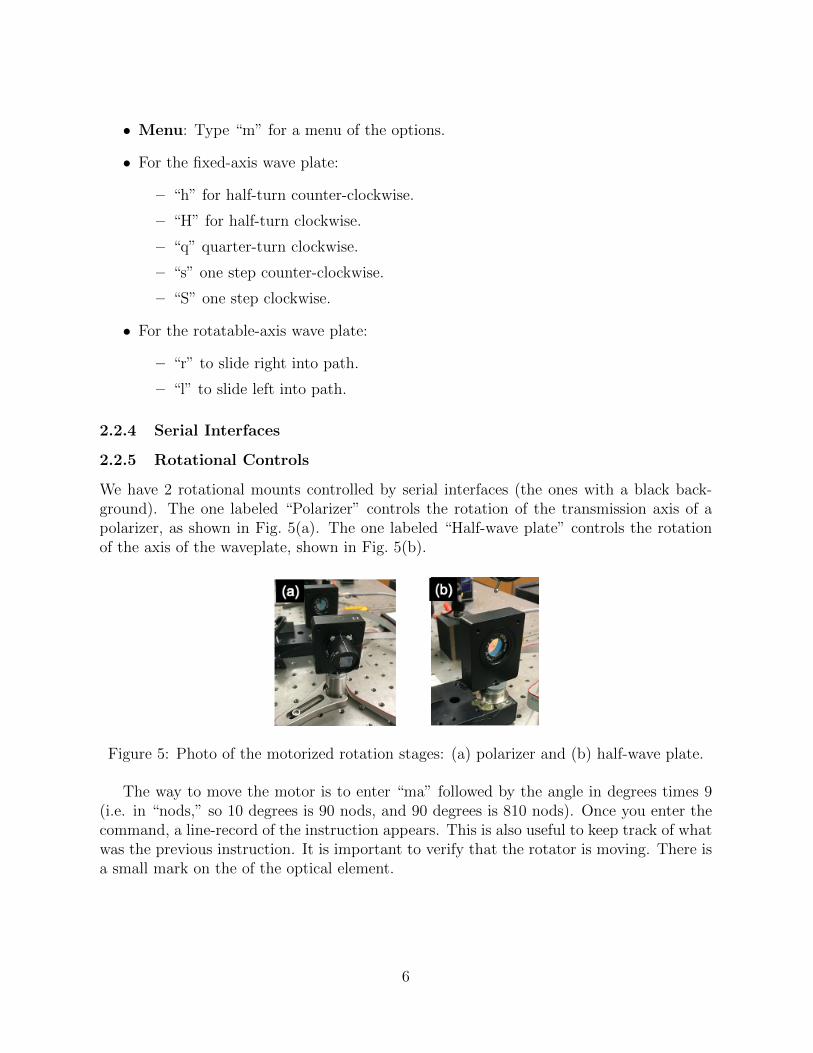
We have 2 rotational mounts controlled by serial interfaces (the ones with a black back-ground). The one labeled “Polarizer” controls the rotation of the transmission axis of apolarizer, as shown in Fig. 5(a). The one labeled “Half-wave plate” controls the rotationof the axis of the waveplate, shown in Fig. 5(b).

Figure 5: Photo of the motorized rotation stages: (a) polarizer and (b) half-wave plate.

The way to move the motor is to enter “ma” followed by the angle in degrees times 9(i.e. in “nods,” so 10 degrees is 90 nods, and 90 degrees is 810 nods). Once you enter thecommand, a line-record of the instruction appears. This is also useful to keep track of whatwas the previous instruction. It is important to verify that the rotator is moving. There isa small mark on the of the optical element.

6

2.3 Matlab Interface

This is the standard Matlab platform that we use to take data. We will use two programs:

• PiezoScan 3Detectors-Altera

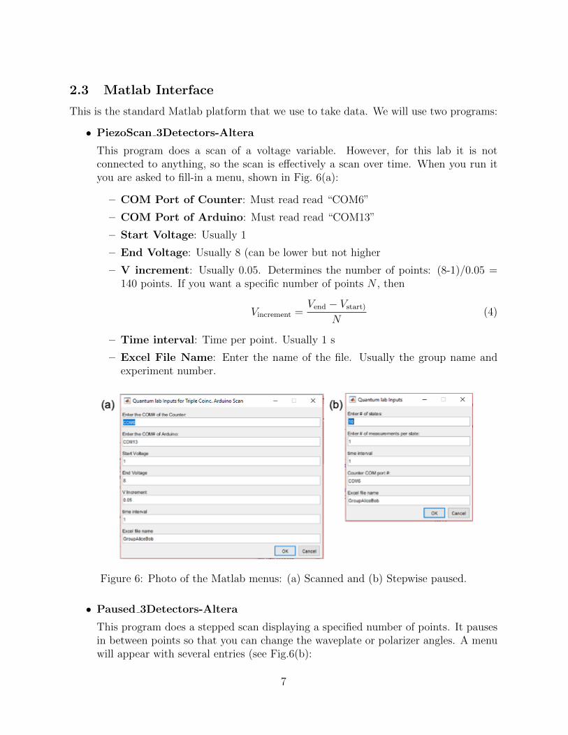
This program does a scan of a voltage variable. However, for this lab it is notconnected to anything, so the scan is effectively a scan over time. When you run ityou are asked to fill-in a menu, shown in Fig. 6(a):

– COM Port of Counter: Must read read “COM6”

– COM Port of Arduino: Must read read “COM13”

– Start Voltage: Usually 1

– End Voltage: Usually 8 (can be lower but not higher

– V increment: Usually 0.05. Determines the number of points: (8-1)/0.05 =140 points. If you want a specific number of points N , then

Vincrement =Vend − Vstart)

N(4)

– Time interval: Time per point. Usually 1 s

– Excel File Name: Enter the name of the file. Usually the group name andexperiment number.

Figure 6: Photo of the Matlab menus: (a) Scanned and (b) Stepwise paused.

• Paused 3Detectors-Altera

This program does a stepped scan displaying a specified number of points. It pausesin between points so that you can change the waveplate or polarizer angles. A menuwill appear with several entries (see Fig.6(b):

7

– COM Port of Counter: Must read read “COM6”

– Number of states: This is the number of measurements you need. You get apause between measurements

– Number of measurements per state: This is number of measurements perpause. Normally set to 1.

– OK button: The program will take a data point after you click this, and thenpause once it is ready to take another point.

– Excel File Name: Enter the name of the file. Usually the group name andexperiment number.

3 Experiments

This lab continues the alignment done the previous lab, where all components were putin place aligned with the alignment beam. In this lab we will do experiments with singlephotons to investigate the properties of quantum mechanics algebra. You will require todo a group lab write-up for this experiment. Members of the group should divide tasks,but all should do the theory part individually. The first step in this experiment is to setup the apparatus to produce spontaneous parametric down conversion. At least one groupmember should keep detailed notes of what you do in a bound notebook (not loose sheetsnor in a random piece of paper).

3.1 Experiment 1: An Overview of the Apparatus

• Task 1: Inspection This is a good point for making a sketch of the apparatus inyour notebook and adding by hand all the details that you can think.

• Task 2: Getting to know all the controls: A walk-through

1. Unblock the alignment laser via the Arduino interface by typing “5”. You shouldsee the scattering of the laser from the optical components. (You can expandthe webcam view to see better.)

2. Rotate the fixed wave plate via the Teensy interface. For example, enter “Q”to put the waveplate into position (the lower position- you will see the laserscattering from it when it is in position). You can enter “q” to return it back tobe out of position.

3. Slide the rotating wave plate into position by entering “r”. You will see it move,taking about 1 minute to complete.

4. Block the alignment laser via the Arduino interface by typing “6”. You shouldno longer se a red glare reflected from the optical components.

8

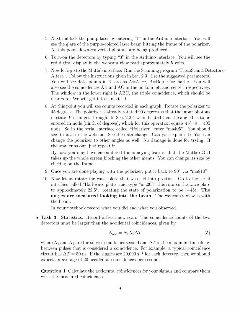
5. Next unblock the pump laser by entering “1” in the Arduino interface. You willsee the glare of the purple-colored laser beam hitting the frame of the polarizer.At this point down-converted photons are being produced.

6. Turn-on the detectors by typing “3” in the Arduino interface. You will see thered digital display in the webcam view read approximately 5 volts.

7. Now let’s go to the Matlab interface. Run the Scanning program “PiezoScan 3Detectors-Altera”. Follow the instructions given in Sec. 2.3. Use the suggested parameters.You will see data points in 6 screens A=Alice, B=Bob, C=Charlie. You willalso see the coincidences AB and AC in the bottom left and center, respectively.The window in the lower right is ABC, the triple coincidence, which should benear zero. We will get into it next lab.

8. At this point you will see counts recorded in each graph. Rotate the polarizer to45 degrees. The polarizer is already rotated 90 degrees so that the input photonsin state |V 〉 can get through. In Sec. 2.2.4 we indicated that the angle has to beentered in nods (ninth of degrees), which for this operation equals 45◦ · 9 = 405nods. So in the serial interface called “Polarizer” enter “ma405”. You shouldsee it move in the webcam. See the data change. Can you explain it? You canchange the polarizer to other angles as well. No damage is done for trying. Ifthe scan runs out, just repeat it.

By now you may have encountered the annoying feature that the Matlab GUItakes up the whole screen blocking the other menus. You can change its size byclicking on the frame.

9. Once you are done playing with the polarizer, put it back to 90◦ via “ma810”.

10. Now let us rotate the wave plate that was slid into position. Go to the serialinterface called “Half-wave plate” and type “ma203” this rotates the wave plateto approximately 22.5◦. rotating the state of polarization to be |−45〉. Theangles are measured looking into the beam. The webcam’s view is withthe beam.

In your notebook record what you did and what you observed.

• Task 3: Statistics. Record a fresh new scan. The coincidence counts of the twodetectors must be larger than the accidental coincidences, given by

Nacc = N1N2∆T, (5)

where N1 and N2 are the singles counts per second and ∆T is the maximum time delaybetween pulses that is considered a coincidence. For example, a typical coincidencecircuit has ∆T = 50 ns. If the singles are 20,000 s−1 for each detector, then we shouldexpect an average of 20 accidental coincidences per second.

Question 1 Calculate the accidental coincidences for your signals and compare themwith the measured coincidences.

9

Question 2 You can consider the statistics to be Poissonian, and so the error in thenumber of recorded counts N , is

√N . Take the average and standard deviation of

the individual counts that you record and compare with√N .

3.2 State Transformation and Detection

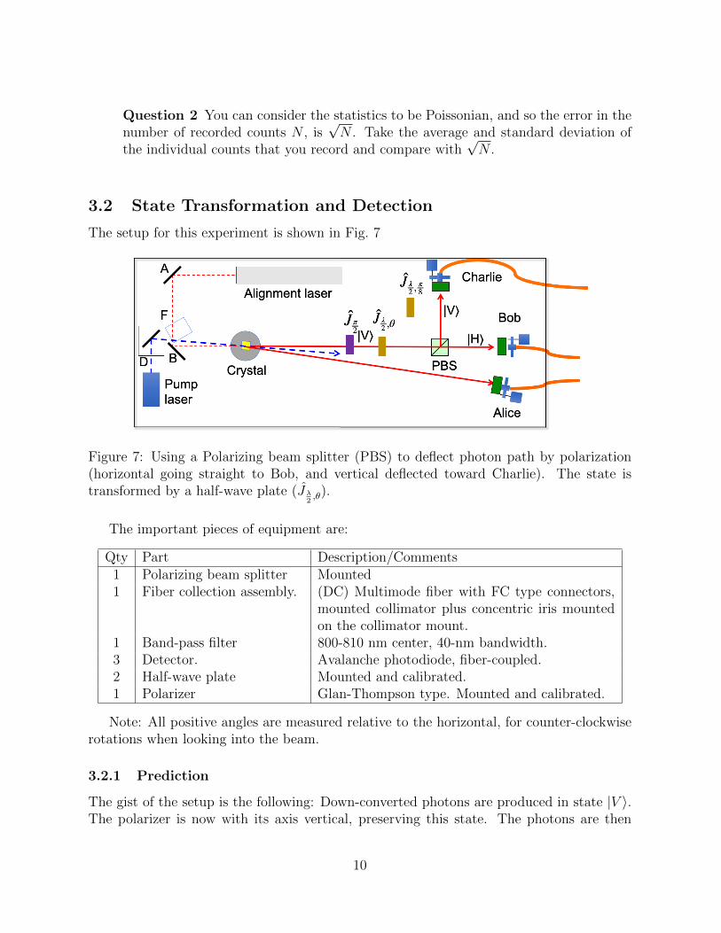
The setup for this experiment is shown in Fig. 7

Figure 7: Using a Polarizing beam splitter (PBS) to deflect photon path by polarization(horizontal going straight to Bob, and vertical deflected toward Charlie). The state istransformed by a half-wave plate (Jλ

2,θ).

The important pieces of equipment are:

Qty Part Description/Comments1 Polarizing beam splitter Mounted1 Fiber collection assembly. (DC) Multimode fiber with FC type connectors,

mounted collimator plus concentric iris mountedon the collimator mount.

1 Band-pass filter 800-810 nm center, 40-nm bandwidth.3 Detector. Avalanche photodiode, fiber-coupled.2 Half-wave plate Mounted and calibrated.1 Polarizer Glan-Thompson type. Mounted and calibrated.

Note: All positive angles are measured relative to the horizontal, for counter-clockwiserotations when looking into the beam.

3.2.1 Prediction

The gist of the setup is the following: Down-converted photons are produced in state |V 〉.The polarizer is now with its axis vertical, preserving this state. The photons are then

10

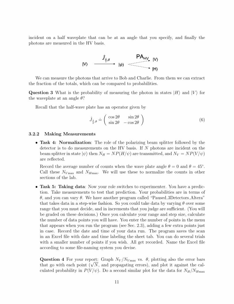
incident on a half waveplate that can be at an angle that you specify, and finally thephotons are measured in the HV basis.

We can measure the photons that arrive to Bob and Charlie. From them we can extractthe fraction of the totals, which can be compared to probabilities.

Question 3 What is the probability of measuring the photon in states |H〉 and |V 〉 forthe waveplate at an angle θ?

Recall that the half-wave plate has an operator given by

Jλ2,θ

.=

(cos 2θ sin 2θsin 2θ − cos 2θ

)(6)

3.2.2 Making Measurements

• Task 4: Normalization: The role of the polarizing beam splitter followed by thedetector is to do measurements on the HV basis. If N photons are incident on thebeam splitter in state |ψ〉 thenNH = NP (H/ψ) are transmitted, andNV = NP (V/ψ)are reflected.

Record the average number of counts when the wave plate angle θ = 0 and θ = 45◦.Call these NVmax and NHmax. We will use these to normalize the counts in othersections of the lab.

• Task 5: Taking data: Now your role switches to experimenter. You have a predic-tion. Take measurements to test that prediction. Your probabilities are in terms ofθ, and you can vary θ. We have another program called “Paused 3Detectors Altera”that takes data in a step-wise fashion. So you could take data by varying θ over somerange that you must decide, and in increments that you judge are sufficient. (You willbe graded on these decisions.) Once you calculate your range and step size, calculatethe number of data points you will have. You enter the number of points in the menuthat appears when you run the program (see Sec. 2.3), adding a few extra points justin case. Record the date and time of your data run. The program saves the scanin an Excel file with date and time labeling the sheet tab. You can do several trialswith a smaller number of points if you wish. All get recorded. Name the Excel fileaccording to some file-naming system you devise.

Question 4 For your report: Graph NV /NVmax vs. θ, plotting also the error barsthat go with each point (

√N , and propagating errors), and plot it against the cal-

culated probability in P (V/ψ). Do a second similar plot for the data for NH/NHmax

11

and the calculated P (H/ψ). Display them in the same graph. Are they what youexpect?

3.3 Polarization Projection

We now want to verify state projection by a polarizer.

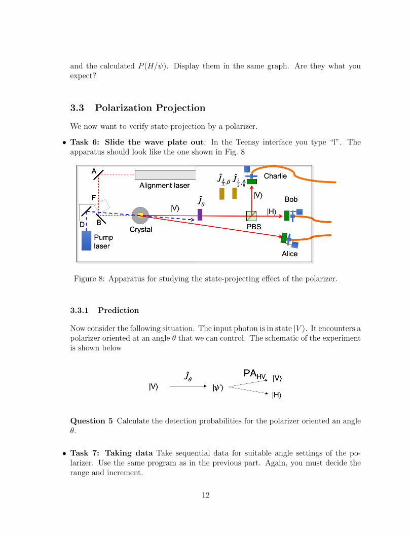
• Task 6: Slide the wave plate out: In the Teensy interface you type “l”. Theapparatus should look like the one shown in Fig. 8

Figure 8: Apparatus for studying the state-projecting effect of the polarizer.

3.3.1 Prediction

Now consider the following situation. The input photon is in state |V 〉. It encounters apolarizer oriented at an angle θ that we can control. The schematic of the experimentis shown below

Question 5 Calculate the detection probabilities for the polarizer oriented an angleθ.

• Task 7: Taking data Take sequential data for suitable angle settings of the po-larizer. Use the same program as in the previous part. Again, you must decide therange and increment.

12

Question 6 Make a graph of the normalized detections on each detector (i.e., HV /NVmax

and HH/NHmax) in the same graph along with theoretical predictions. Measurementsshould be symbols with error bars and theory/expectation should be a continuousline. Explain the graph and the action of the polarizer.

3.4 45-Degree Basis

We can also analyze the photons in a different basis. Here we will use the 45-degree basis.

• Task 8: Setting the 45 Basis: There are several steps:

– Set the polarizer to 90◦.

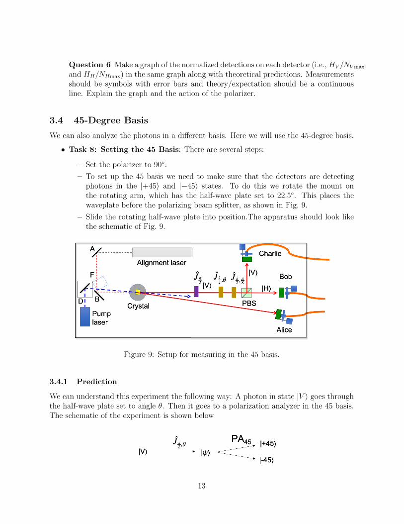
– To set up the 45 basis we need to make sure that the detectors are detectingphotons in the |+45〉 and |−45〉 states. To do this we rotate the mount onthe rotating arm, which has the half-wave plate set to 22.5◦. This places thewaveplate before the polarizing beam splitter, as shown in Fig. 9.

– Slide the rotating half-wave plate into position.The apparatus should look likethe schematic of Fig. 9.

Figure 9: Setup for measuring in the 45 basis.

3.4.1 Prediction

We can understand this experiment the following way: A photon in state |V 〉 goes throughthe half-wave plate set to angle θ. Then it goes to a polarization analyzer in the 45 basis.The schematic of the experiment is shown below

13

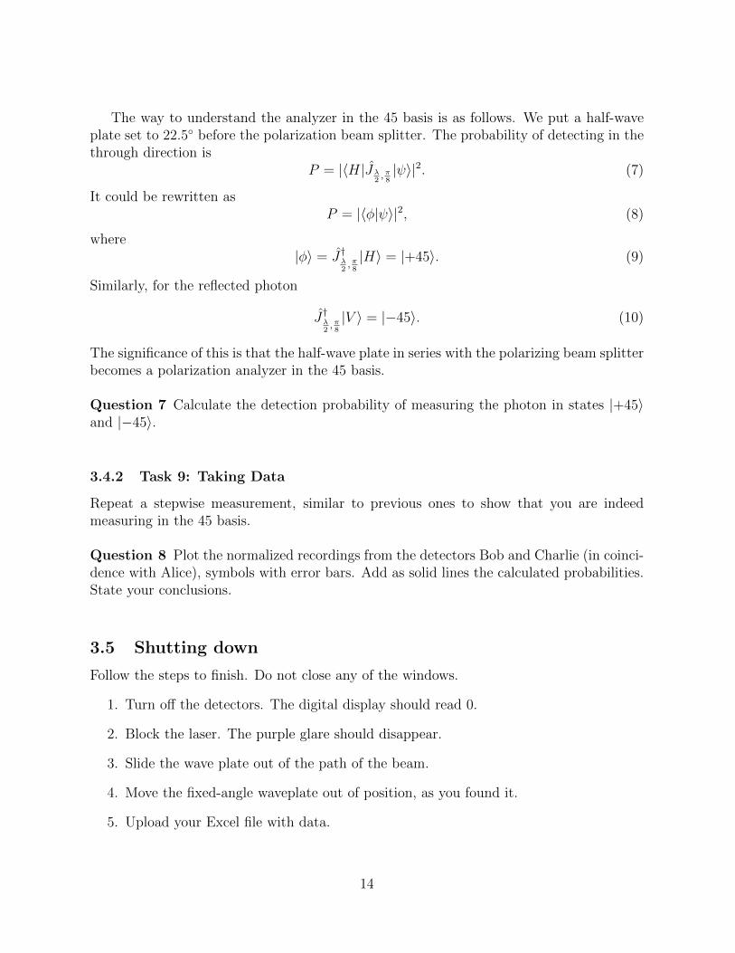
The way to understand the analyzer in the 45 basis is as follows. We put a half-waveplate set to 22.5◦ before the polarization beam splitter. The probability of detecting in thethrough direction is

P = |〈H|Jλ2,π8|ψ〉|2. (7)

It could be rewritten asP = |〈φ|ψ〉|2, (8)

where|φ〉 = J†λ

2,π8

|H〉 = |+45〉. (9)

Similarly, for the reflected photon

J†λ2,π8

|V 〉 = |−45〉. (10)

The significance of this is that the half-wave plate in series with the polarizing beam splitterbecomes a polarization analyzer in the 45 basis.

Question 7 Calculate the detection probability of measuring the photon in states |+45〉and |−45〉.

3.4.2 Task 9: Taking Data

Repeat a stepwise measurement, similar to previous ones to show that you are indeedmeasuring in the 45 basis.

Question 8 Plot the normalized recordings from the detectors Bob and Charlie (in coinci-dence with Alice), symbols with error bars. Add as solid lines the calculated probabilities.State your conclusions.

3.5 Shutting down

Follow the steps to finish. Do not close any of the windows.

1. Turn off the detectors. The digital display should read 0.

2. Block the laser. The purple glare should disappear.

3. Slide the wave plate out of the path of the beam.

4. Move the fixed-angle waveplate out of position, as you found it.

5. Upload your Excel file with data.

14