UVA CS 4774: Machine Learning Lecture 5: Linear Regression ...
31
UVA CS 4774: Machine Learning Lecture 5: Linear Regression with Basis Functions Expansion Dr. Yanjun Qi University of Virginia Department of Computer Science 9/10/20 Dr. Yanjun Qi / UVA CS 1
Transcript of UVA CS 4774: Machine Learning Lecture 5: Linear Regression ...
UVA CS 4774:Machine Learning
Lecture 5: Linear Regression with Basis Functions Expansion
Dr. Yanjun Qi
University of Virginia Department of Computer Science
9/10/20 Dr. Yanjun Qi / UVA CS 1
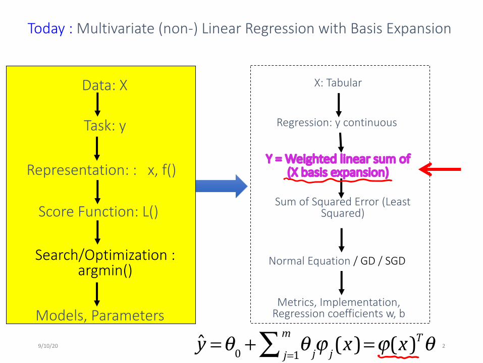
Today : Multivariate (non-) Linear Regression with Basis Expansion
Regression: y continuous
Y = Weighted linear sum of (X basis expansion)
Sum of Squared Error (Least Squared)
Normal Equation / GD / SGD
Metrics, Implementation, Regression coefficients w, b
9/10/20 2
Task: y
Representation: : x, f()
Score Function: L()
Search/Optimization : argmin()
Models, Parameters
Data: X X: Tabular
!! y =θ0 + θ jϕ j(x)j=1m∑ =ϕ(x)Tθ
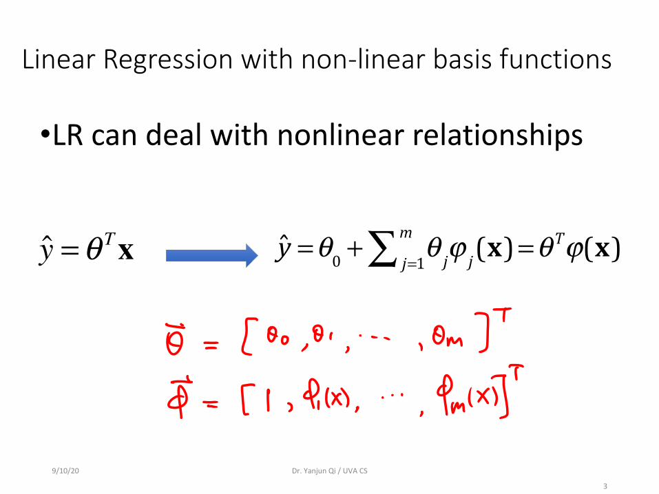
Linear Regression with non-linear basis functions
•LR can deal with nonlinear relationships
9/10/20 Dr. Yanjun Qi / UVA CS
3
y =θ0 + θ jϕ j(x)j=1m∑ =θTϕ(x)y =θ Tx
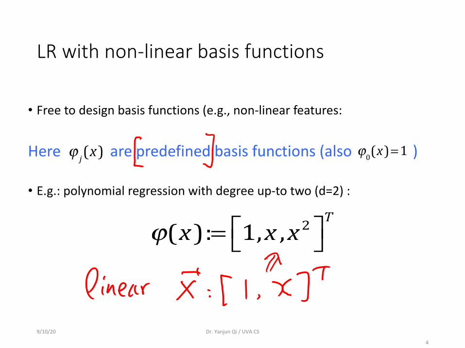
LR with non-linear basis functions
• Free to design basis functions (e.g., non-linear features:
Here are predefined basis functions (also )
• E.g.: polynomial regression with degree up-to two (d=2) :
9/10/20 Dr. Yanjun Qi / UVA CS
4
ϕ(x):= 1,x ,x2⎡⎣ ⎤⎦T
!!ϕ j(x) !!ϕ0(x)=1
Polynomial basis based Regression
9/10/20 Dr. Yanjun Qi / UVA CS 5
9/10/20 Dr. Yanjun Qi / UVA CS 6
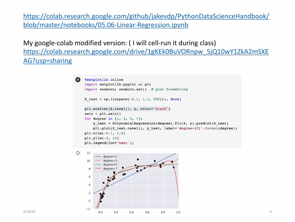
https://colab.research.google.com/github/jakevdp/PythonDataScienceHandbook/blob/master/notebooks/05.06-Linear-Regression.ipynb
My google-colab modified version: ( I will cell-run it during class)https://colab.research.google.com/drive/1gKEk0BuVORnpw_5jQ10wY1ZkA2mSXEAG?usp=sharing
9/10/20 7
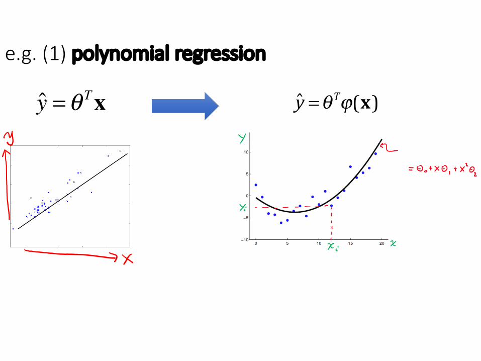
e.g. (1) polynomial regression
θ * = ϕTϕ( )−1ϕT !y( ) yXXX TT !1-
=*q
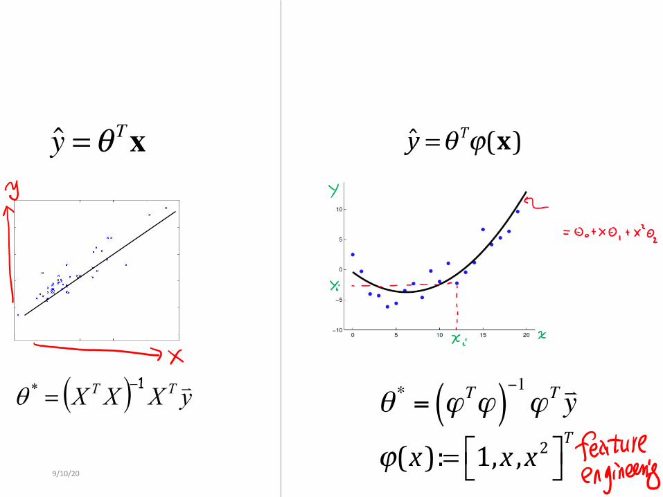
y =θTϕ(x)y =θ Tx
ϕ(x):= 1,x ,x2⎡⎣ ⎤⎦T
9/10/20 8
θ * = ϕTϕ( )−1ϕT !y( ) yXXX TT !1-
=*q
y =θTϕ(x)y =θ Tx
ϕ(x):= 1,x ,x2⎡⎣ ⎤⎦T
9/10/20 9
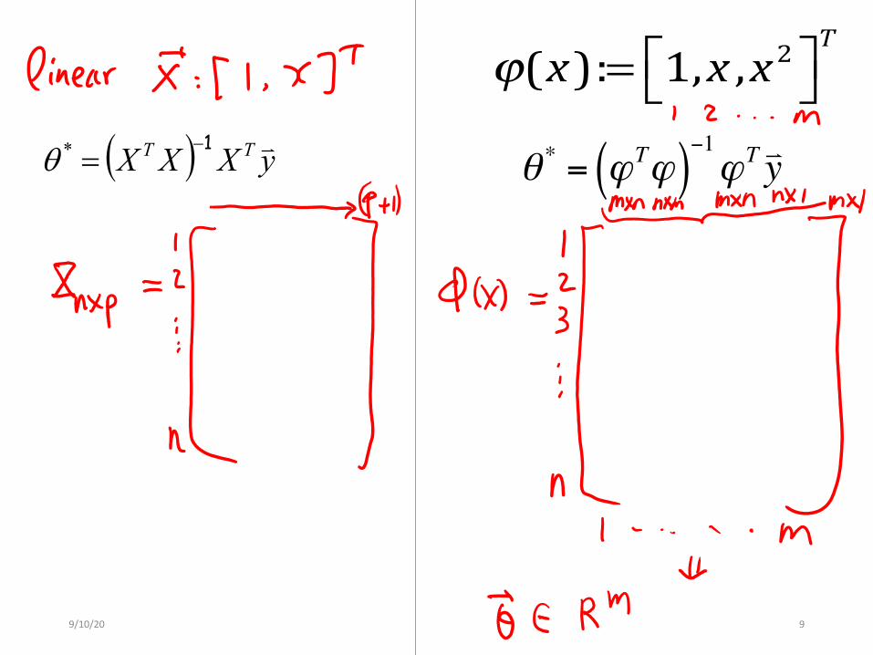
ϕ(x):= 1,x ,x2⎡⎣ ⎤⎦T
θ * = ϕTϕ( )−1ϕT !y( ) yXXX TT !1-
=*q
9/10/20 Dr. Yanjun Qi / UVA CS 10
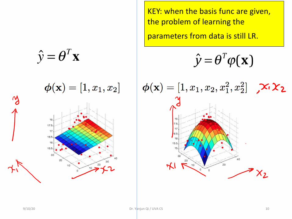
KEY: when the basis func are given, the problem of learning the
parameters from data is still LR.
y =θTϕ(x)y =θ Tx
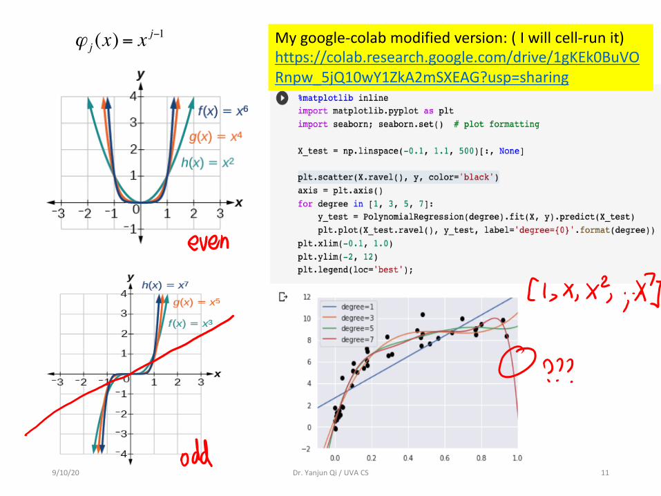
9/10/20 Dr. Yanjun Qi / UVA CS 11
ϕ j (x) = xj−1 My google-colab modified version: ( I will cell-run it)
https://colab.research.google.com/drive/1gKEk0BuVORnpw_5jQ10wY1ZkA2mSXEAG?usp=sharing
UVA CS 4774:Machine Learning
Lecture 5: Linear Regression with Basis Functions Expansion
Dr. Yanjun Qi
University of Virginia Department of Computer Science
9/10/20 Dr. Yanjun Qi / UVA CS 12
Module 2
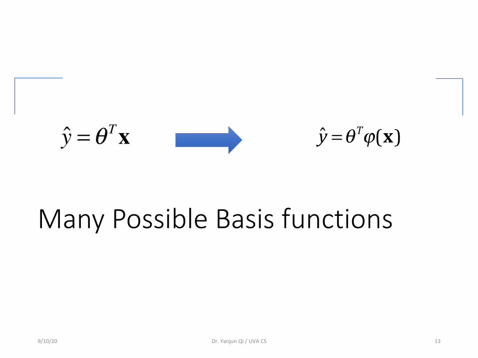
Many Possible Basis functions
9/10/20 Dr. Yanjun Qi / UVA CS 13
y =θTϕ(x)y =θ Tx
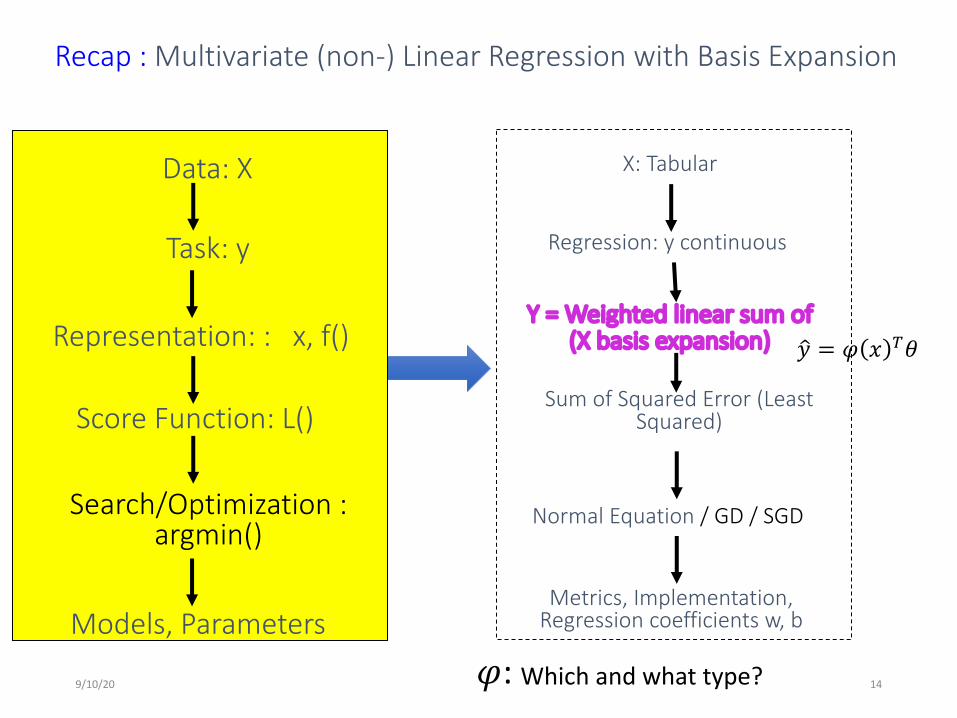
Recap : Multivariate (non-) Linear Regression with Basis Expansion
Regression: y continuous
Y = Weighted linear sum of (X basis expansion)
Sum of Squared Error (Least Squared)
Normal Equation / GD / SGD
Metrics, Implementation, Regression coefficients w, b
9/10/20 14
Task: y
Representation: : x, f()
Score Function: L()
Search/Optimization : argmin()
Models, Parameters
Data: X X: Tabular
𝜑: Which and what type?
!𝑦 = 𝜑 𝑥 !𝜃
9/10/20 Dr. Yanjun Qi / UVA CS
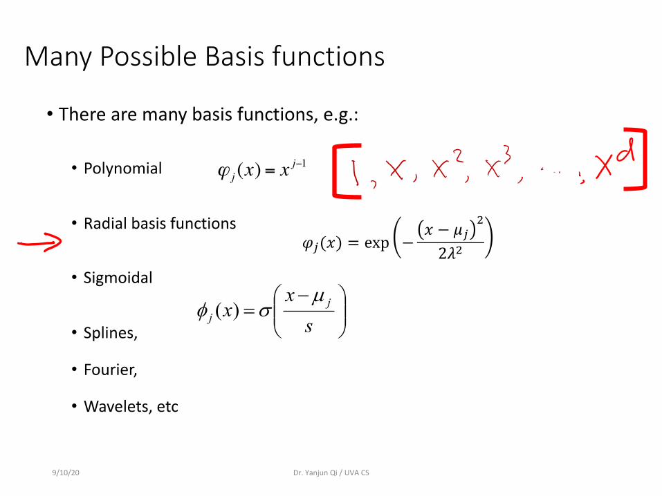
Many Possible Basis functions
• There are many basis functions, e.g.:
• Polynomial
• Radial basis functions
• Sigmoidal
• Splines,
• Fourier,
• Wavelets, etc
ϕ j (x) = xj−1
÷÷ø
öççè
æ -=
sx
x jj
µsf )(
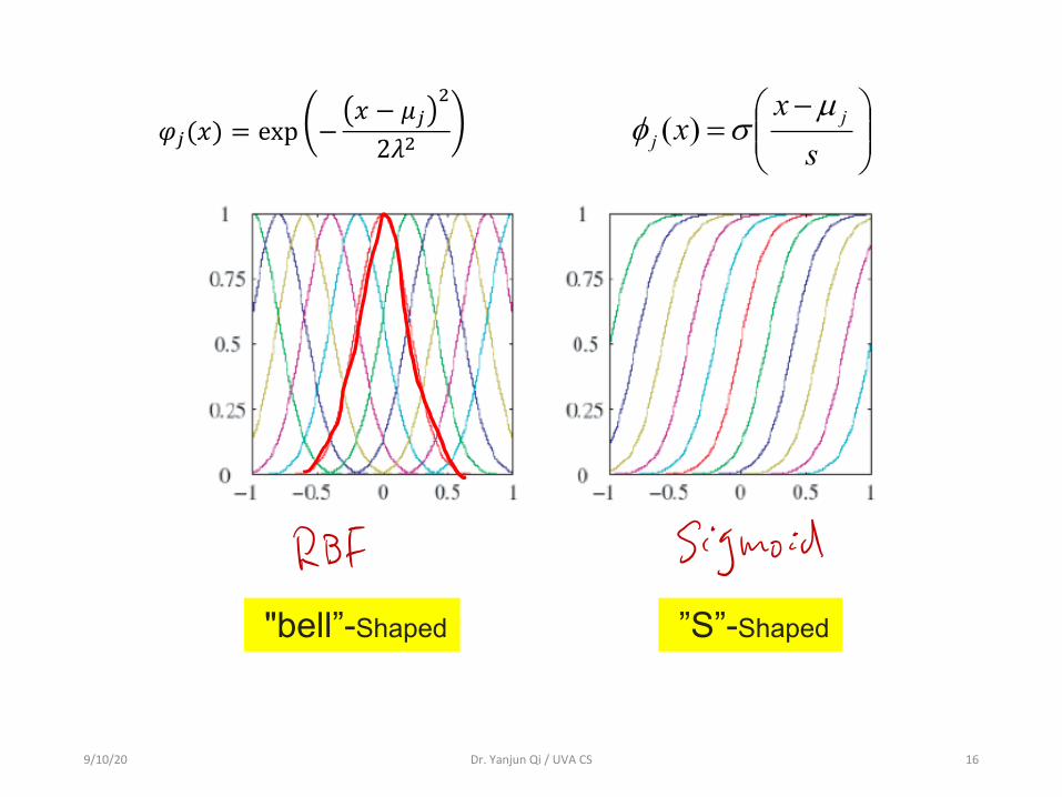
𝜑"(𝑥) = exp −𝑥 − 𝜇"
#
2𝜆#
9/10/20 Dr. Yanjun Qi / UVA CS 16
𝜑"(𝑥) = exp −𝑥 − 𝜇"
#
2𝜆# ÷÷ø
öççè
æ -=
sx
x jj
µsf )(
"bell”-Shaped ”S”-Shaped
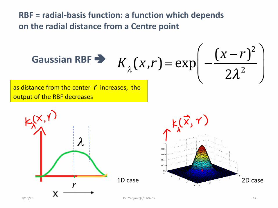
Kλ(x ,r)= exp − (x − r)
2
2λ2⎛
⎝⎜⎞
⎠⎟
RBF = radial-basis function: a function which dependson the radial distance from a Centre point
Gaussian RBF è
as distance from the center r increases, the output of the RBF decreases
1D case 2D case
9/10/20 Dr. Yanjun Qi / UVA CS 17
9/10/20 Dr. Yanjun Qi / UVA CS 18
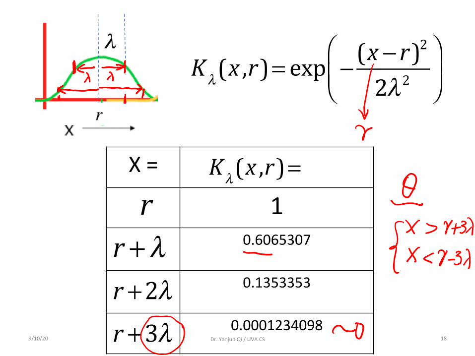
Kλ(x ,r)= exp − (x − r)
2
2λ2⎛
⎝⎜⎞
⎠⎟
X =
10.6065307
0.1353353
0.0001234098
Kλ(x ,r)=r
r +λ
r +2λr +3λ
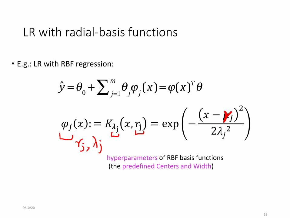
LR with radial-basis functions
• E.g.: LR with RBF regression:
9/10/20
19
!! y =θ0 + θ jϕ j(x)j=1m∑ =ϕ(x)Tθ
𝜑! 𝑥 := 𝐾"! 𝑥, 𝑟# = exp −𝑥 − 𝜇!
$
2𝜆𝑗$
hyperparameters of RBF basis functions(the predefined Centers and Width)
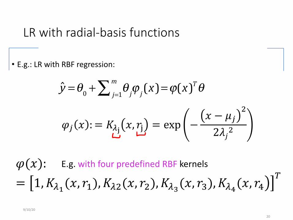
LR with radial-basis functions
• E.g.: LR with RBF regression:
9/10/20
20
!! y =θ0 + θ jϕ j(x)j=1m∑ =ϕ(x)Tθ
𝜑! 𝑥 := 𝐾"! 𝑥, 𝑟# = exp −𝑥 − 𝜇!
$
2𝜆𝑗$
𝜑(𝑥):= '1, 𝐾!"(𝑥, 𝑟"), 𝐾!#(𝑥, 𝑟#), 𝐾!#(𝑥, 𝑟$), 𝐾!$(𝑥, 𝑟%
&E.g. with four predefined RBF kernels
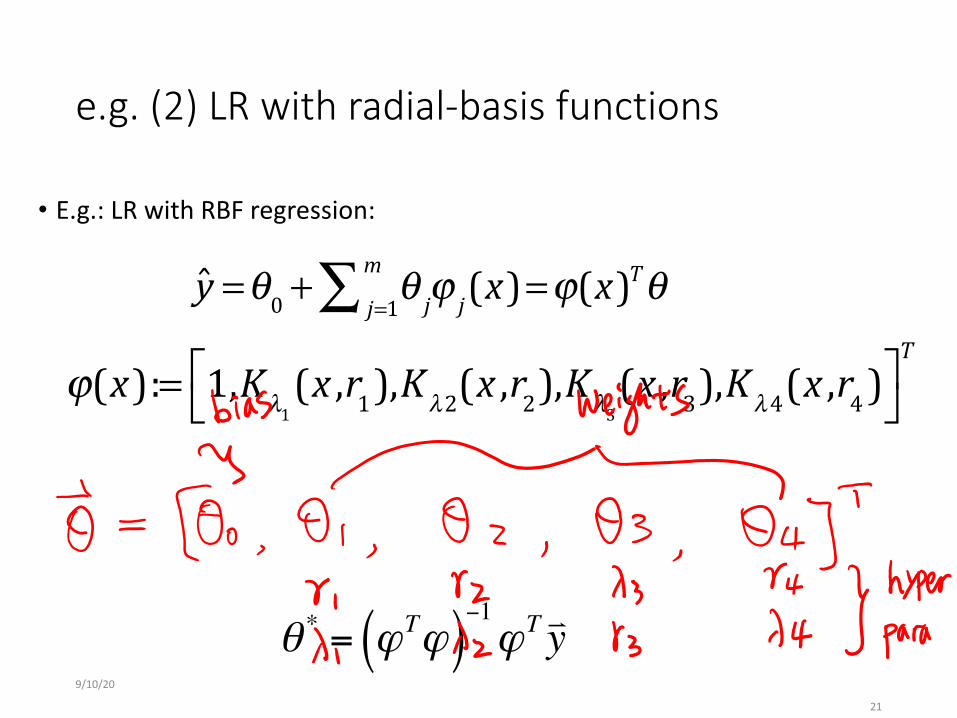
e.g. (2) LR with radial-basis functions
• E.g.: LR with RBF regression:
9/10/20
21
!! y =θ0 + θ jϕ j(x)j=1m∑ =ϕ(x)Tθ
!!ϕ(x):= 1,Kλ1(x ,r1),Kλ2(x ,r2),Kλ3
(x ,r3),Kλ4(x ,r4 )⎡⎣
⎤⎦T
θ * = ϕTϕ( )−1ϕT !y
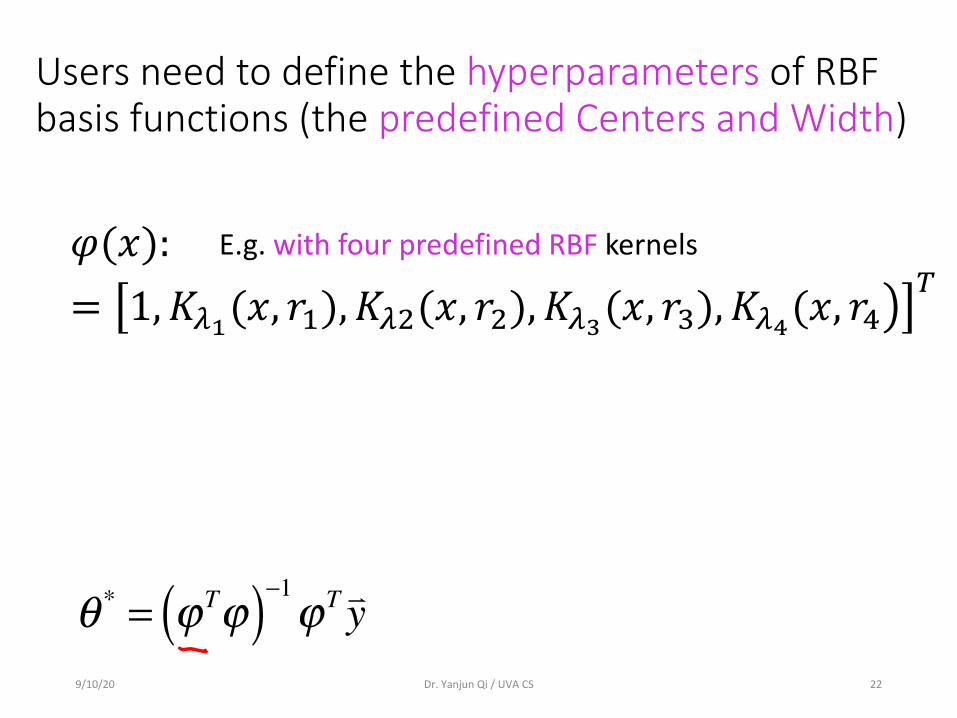
Users need to define the hyperparameters of RBF basis functions (the predefined Centers and Width)
9/10/20 Dr. Yanjun Qi / UVA CS 22
θ * = ϕTϕ( )−1ϕT !y
𝜑(𝑥):= '1, 𝐾!"(𝑥, 𝑟"), 𝐾!#(𝑥, 𝑟#), 𝐾!#(𝑥, 𝑟$), 𝐾!$(𝑥, 𝑟%
&E.g. with four predefined RBF kernels
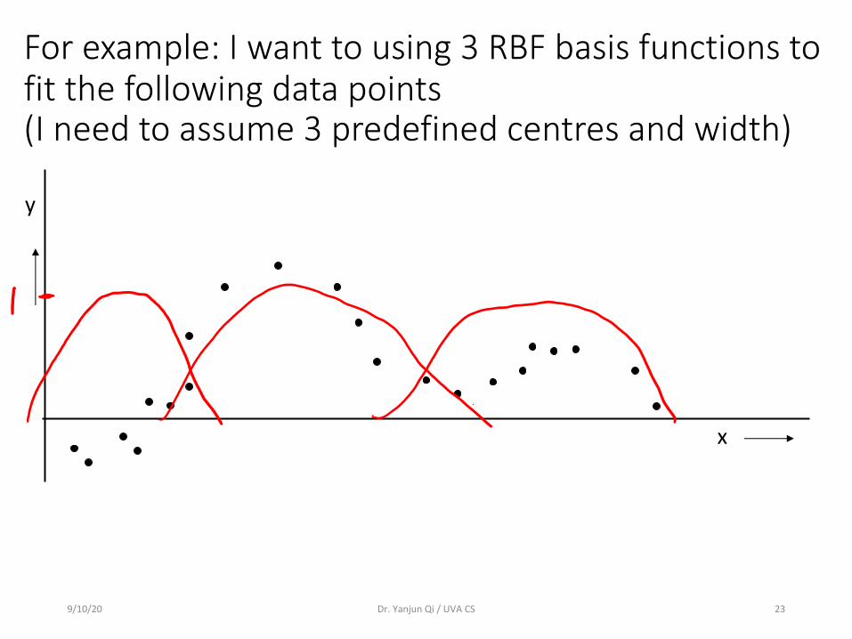
9/10/20 Dr. Yanjun Qi / UVA CS 23
x
y
For example: I want to using 3 RBF basis functions to fit the following data points (I need to assume 3 predefined centres and width)
9/10/20 Dr. Yanjun Qi / UVA CS 24
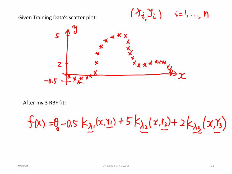
After my 3 RBF fit:
Given Training Data’s scatter plot:
9/10/20 Dr. Yanjun Qi / UVA CS 25
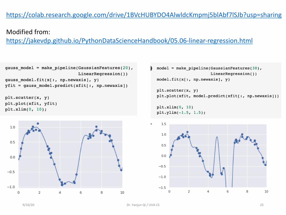
https://colab.research.google.com/drive/1BVcHUBYDO4AlwldcKmpmj5blAbf7lSJb?usp=sharing
Modified from: https://jakevdp.github.io/PythonDataScienceHandbook/05.06-linear-regression.html
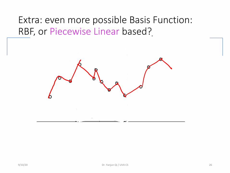
Extra: even more possible Basis Function: RBF, or Piecewise Linear based?
9/10/20 Dr. Yanjun Qi / UVA CS 26
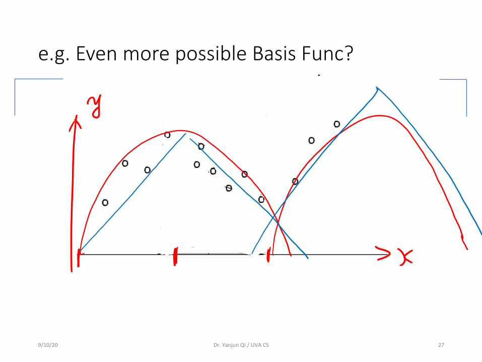
e.g. Even more possible Basis Func?
9/10/20 Dr. Yanjun Qi / UVA CS 27
Thank you
28
Thank You
9/10/20

Extra
9/10/20 Dr. Yanjun Qi / UVA CS 29
9/10/20
30
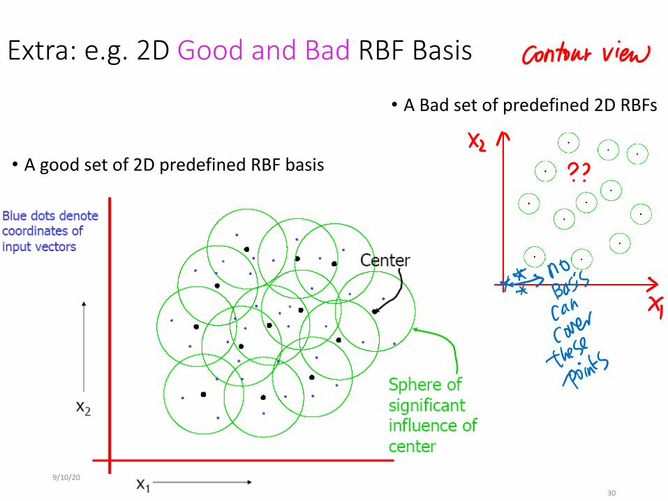
Extra: e.g. 2D Good and Bad RBF Basis
• A good set of 2D predefined RBF basis
• A Bad set of predefined 2D RBFs
Extra: Nonparametric Regression Models
• K-Nearest Neighbor (KNN) and Locally weighted linear regression are non-parametric algorithms.
• The (unweighted) linear regression algorithm that we saw earlier is known as a parametric learning algorithm • because it has a fixed, finite number of parameters which are fit to the data;• Once we've fit the \theta and stored them away, we no longer need to keep
the training data around to make future predictions.• In contrast, to make predictions using KNN or locally weighted linear
regression, we need to keep the entire training set around.
• The term "non-parametric" (roughly) refers to the fact that the amount of knowledge we need to keep, in order to represent the hypothesis grows with linearly the size of the training set.
9/10/20 Dr. Yanjun Qi / UVA CS 31