Multivariate Logistic Regression - McGill · PDF file1 Multivariate Logistic Regression As in...
21
1 Multivariate Logistic Regression As in univariate logistic regression, let π(x) represent the probability of an event that depends on p covariates or independent variables. Then, using an inv.logit formulation for modeling the probability, we have: π(x)= e β 0 +β 1 X 1 +β 2 X 2 +...+βpXp 1+ e β 0 +β 1 X 1 +β 2 X 2 +...+βpXp So, the form is identical to univariate logistic regression, but now with more than one covariate. [Note: by “univariate” logistic regression, I mean logistic regression with one independent variable; really there are two variables involved, the independent variable and the dichotomous outcome, so it could also be termed bivariate.] To obtain the corresponding logit function from this, we calculate (letting X represent the whole set of covariates X 1 ,X 2 ,...,X p ): logit[π(X )] = ln π(X ) 1 - π(X ) = ln e β 0 +β 1 X 1 +β 2 X 2 +...+βpXp 1+e β 0 +β 1 X 1 +β 2 X 2 +...+βpXp 1 - e β 0 +β 1 X 1 +β 2 X 2 +...+βpXp 1+e β 0 +β 1 X 1 +β 2 X 2 +...+βpXp = ln e β 0 +β 1 X 1 +β 2 X 2 +...+βpXp 1+e β 0 +β 1 X 1 +β 2 X 2 +...+βpXp 1 1+e β 0 +β 1 X 1 +β 2 X 2 +...+βpXp = ln e β 0 +β 1 X 1 +β 2 X 2 +...+βpXp = β 0 + β 1 X 1 + β 2 X 2 + ... + β p X p So, again, we see that the logit of the probability of an event given X is a simple linear function.
Transcript of Multivariate Logistic Regression - McGill · PDF file1 Multivariate Logistic Regression As in...
1
Multivariate Logistic Regression
As in univariate logistic regression, let π(x) represent the probability of an event thatdepends on p covariates or independent variables. Then, using an inv.logit formulationfor modeling the probability, we have:
π(x) =eβ0+β1X1+β2X2+...+βpXp
1 + eβ0+β1X1+β2X2+...+βpXp
So, the form is identical to univariate logistic regression, but now with more than onecovariate. [Note: by “univariate” logistic regression, I mean logistic regression withone independent variable; really there are two variables involved, the independentvariable and the dichotomous outcome, so it could also be termed bivariate.]
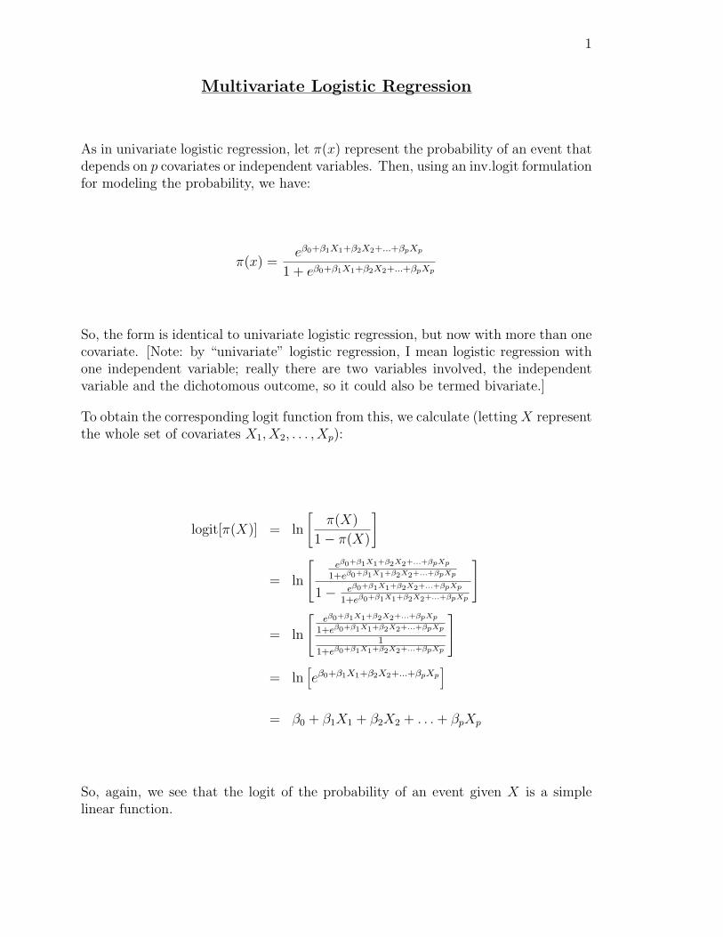
To obtain the corresponding logit function from this, we calculate (letting X representthe whole set of covariates X1, X2, . . . , Xp):
logit[π(X)] = ln
[π(X)
1− π(X)
]
= ln
eβ0+β1X1+β2X2+...+βpXp
1+eβ0+β1X1+β2X2+...+βpXp
1− eβ0+β1X1+β2X2+...+βpXp
1+eβ0+β1X1+β2X2+...+βpXp
= ln
eβ0+β1X1+β2X2+...+βpXp
1+eβ0+β1X1+β2X2+...+βpXp
11+eβ0+β1X1+β2X2+...+βpXp
= ln
[eβ0+β1X1+β2X2+...+βpXp
]= β0 + β1X1 + β2X2 + . . . + βpXp
So, again, we see that the logit of the probability of an event given X is a simplelinear function.
2
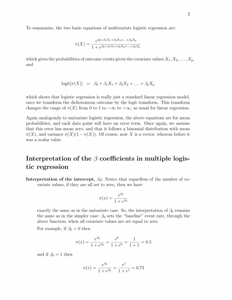
To summarize, the two basic equations of multivariate logistic regression are:
π(X) =eβ0+β1X1+β2X2+...+βpXp
1 + eβ0+β1X1+β2X2+...+βpXp
which gives the probabilities of outcome events given the covariate values X1, X2, . . . , Xp,and
logit[π(X)] = β0 + β1X1 + β2X2 + . . . + βpXp
which shows that logistic regression is really just a standard linear regression model,once we transform the dichotomous outcome by the logit transform. This transformchanges the range of π(X) from 0 to 1 to −∞ to +∞, as usual for linear regression.
Again analogously to univariate logistic regression, the above equations are for meanprobabilities, and each data point will have an error term. Once again, we assumethat this error has mean zero, and that it follows a binomial distribution with meanπ(X), and variance π(X)(1− π(X)). Of course, now X is a vector, whereas before itwas a scalar value.
Interpretation of the β coefficients in multiple logis-
tic regression
Interpretation of the intercept, β0: Notice that regardless of the number of co-variate values, if they are all set to zero, then we have
π(x) =eβ0
1 + eβ0
exactly the same as in the univariate case. So, the interpretation of β0 remainsthe same as in the simpler case: β0 sets the “baseline” event rate, through theabove function, when all covariate values are set equal to zero.
For example, if β0 = 0 then
π(x) =eβ0
1 + eβ0=
e0
1 + e0=
1
1 + 1= 0.5
and if β0 = 1 then
π(x) =eβ0
1 + eβ0=
e1
1 + e1= 0.73

3
and if β0 = −1 then
π(x) =eβ0
1 + eβ0=
e−1
1 + e−1= 0.27
and so on.
As before, positive values of β0 give values greater than 0.5, while negativevalues of β0 give probabilities less than 0.5, when all covariates are set to zero.
Interpretation of the slopes, β1, β2, . . . , βp: Recall the effect on the proba-bility of an event as X changes by one unit in the univariate case. There, wesaw that the coefficient β1 is such that eβ1 is the odds ratio for a unit change in
X, and in general, for a change of z units, the OR = ezβ1 =(eβ1
)z.
Nothing much changes for the multivariate case, except:
• When there is more than one independent variable, if all variables arecompletely uncorrelated with each other, then the interpretations of allcoefficients are simple, and follow the above pattern:
We have OR = ezβi for any variable Xi, i = 1, 2, . . . , p, where the ORrepresents the odds ratio for a change of size z for that variable.
• When the variables are not uncorrelated, the interpretation is more diffi-cult. It is common to say that OR = ezβi represents the odds ratio fora change of size z for that variable adjusted for the effects of the othervariables. While this is essentially correct, we must keep in mind thatconfounding and collinearity can change and obscure these estimated rela-tionships. The way confounding operates is identical to what we saw forlinear regression.
Estimating the β coefficients given a data set
As in the univariate case, the distribution associated with logistic regression is thebinomial. For a single subject with covariate values xi = {x1i, x2i, . . . , xpi}, the like-lihood function is:
π(xi)yi
(1− π(xi))1−yi
For n subjects, the likelihood function is:
n∏i=1
π(xi)yi
(1− π(xi))1−yi
4
To derive estimates of the unknown β parameters, as in the univariate case, we needto maximize this likelihood function. We follow the usual steps, including taking thelogarithm of the likelihood function, taking (p + 1) partial derivatives with respectto each β parameter and setting these (p + 1) equations equal to zero, to form a setof (p + 1) equations in (p + 1) unknowns. Solving this system of equations gives themaximum likelihood equations.
We again omit the details here (as in the univariate case, no easy closed form formulaeexists), and will rely on statistical software to find the maximum likelihood estimatesfor us.
Inferences typically rely on SE formulae for confidence intervals, and likelihood ratiotesting for hypothesis tests. Again, we will omit the details, and rely on statisticalsoftware.
We next look at several examples.
Multiple Logistic Regression Examples
We will look at three examples:
• Logistic regression with dummy or indicator variables
• Logistic regression with many variables
• Logistic regression with interaction terms
In all cases, we will follow a similar procedure to that followed for multiple linearregression:
1. Look at various descriptive statistics to get a feel for the data. For logisticregression, this usually includes looking at descriptive statistics, for examplewithin “outcome = yes = 1” versus “outcome = no = 0” subgroups.
2. The above “by outcome group” descriptive statistics are often sufficient fordiscrete covariates, but you may want to prepare some graphics for continuousvariables. Recall that we did this for the age variable when looking at the CHDexample.
3. For all continuous variables being considered, calculate a correlation matrix ofeach variable against each other variable. This allows one to begin to investigatepossible confounding and collinearity.
5
4. Similarly, for each categorical/continous independent variable pair, look at thevalues for the continuous variable in each category of the other variable.
5. Finally, create tables for all categorical/categorical independent variable pairs.
6. Perform a separate univariate logistic regression for each independent variable.This begins to investigate confounding (we will see in more detail next class),as well as providing an initial “unadjusted” view of the importance of eachvariable, by itself.
7. Think about any “interaction terms” that you may want to try in the model.
8. Perform some sort of model selection technique, or, often much better, thinkabout avoiding any strict model selection by finding a set of models that seemto have something to contribute to overall conclusions.
9. Based on all work done, draw some inferences and conclusions. Carefully inter-pret each estimated parameter, perform “model criticism”, possibly repeatingsome of the above steps (for example, run further models), as needed.
10. Other inferences, such as predictions for future observations, and so on.
As with linear regression, the above should not be considered as “rules”, but ratheras a rough guide as to how to proceed through a logistic regression analysis.
Logistic regression with dummy or indicator variables
Chapter 1 (section 1.6.1) of the Hosmer and Lemeshow book described a data setcalled ICU. Deleting the ID variable, there are 20 variables in this data set, which wedescribe in the table below:

6
Description Coding variable nameVital Status 0 = Lived STA(Main outcome) 1 = DiedAge Years AGESex 0 = Male SEX
1 = FemaleRace 1 = White RACE
2 = Black3 = Other
Service at ICU Admission 0 = Medical SER1 = Surgical
Cancer Part of Present 0 = No CANProblem 1 = YesHistory of Chronic Renal O = No CRNFailure 1 = YesInfection Probable at ICU 0 = No INFAdmission 1 = YesCPR Prior to ICU Admission 0 = No CPR
1 = YesSystolic Blood Pressure at mm Hg SYSICU AdmissionHeart Rate at ICU Admission Beats/min HRAPrevious Admission to an ICU 0 = No PREwithin 6 Months 1 = YesType of Admission 0 = Elective TYP
1 = EmergencyLong Bone, Multiple, Neck, 0 = No FRASingle Area, or Hip Fracture 1 = YesPO2 from Initial Blood Gases 0 > 60 PO2
1 ≤ 60PH from Initial Blood Gases 0 ≥ 7.25 PH
1 < 7.25PCO2 from initial Blood 0 ≤ 45 PCOGases 1 > 45Bicarbonate from Initial 0 ≥ 18 BICBlood Gases 1 < 18Creatinine from Initial Blood 0 ≤ 2.0 CREGases 1 > 2.0Level of Consciousness at ICU O = No Coma LOCAdmission or Stupor
1 = Deepstupor2 = Coma
7
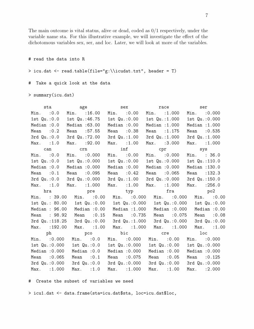
The main outcome is vital status, alive or dead, coded as 0/1 respectively, under thevariable name sta. For this illustrative example, we will investigate the effect of thedichotomous variables sex, ser, and loc. Later, we will look at more of the variables.
# read the data into R
> icu.dat <- read.table(file="g:\\icudat.txt", header = T)
# Take a quick look at the data
> summary(icu.dat)
sta age sex race ser
Min. :0.0 Min. :16.00 Min. :0.00 Min. :1.000 Min. :0.000
1st Qu.:0.0 1st Qu.:46.75 1st Qu.:0.00 1st Qu.:1.000 1st Qu.:0.000
Median :0.0 Median :63.00 Median :0.00 Median :1.000 Median :1.000
Mean :0.2 Mean :57.55 Mean :0.38 Mean :1.175 Mean :0.535
3rd Qu.:0.0 3rd Qu.:72.00 3rd Qu.:1.00 3rd Qu.:1.000 3rd Qu.:1.000
Max. :1.0 Max. :92.00 Max. :1.00 Max. :3.000 Max. :1.000
can crn inf cpr sys
Min. :0.0 Min. :0.000 Min. :0.00 Min. :0.000 Min. : 36.0
1st Qu.:0.0 1st Qu.:0.000 1st Qu.:0.00 1st Qu.:0.000 1st Qu.:110.0
Median :0.0 Median :0.000 Median :0.00 Median :0.000 Median :130.0
Mean :0.1 Mean :0.095 Mean :0.42 Mean :0.065 Mean :132.3
3rd Qu.:0.0 3rd Qu.:0.000 3rd Qu.:1.00 3rd Qu.:0.000 3rd Qu.:150.0
Max. :1.0 Max. :1.000 Max. :1.00 Max. :1.000 Max. :256.0
hra pre typ fra po2
Min. : 39.00 Min. :0.00 Min. :0.000 Min. :0.000 Min. :0.00
1st Qu.: 80.00 1st Qu.:0.00 1st Qu.:0.000 1st Qu.:0.000 1st Qu.:0.00
Median : 96.00 Median :0.00 Median :1.000 Median :0.000 Median :0.00
Mean : 98.92 Mean :0.15 Mean :0.735 Mean :0.075 Mean :0.08
3rd Qu.:118.25 3rd Qu.:0.00 3rd Qu.:1.000 3rd Qu.:0.000 3rd Qu.:0.00
Max. :192.00 Max. :1.00 Max. :1.000 Max. :1.000 Max. :1.00
ph pco bic cre loc
Min. :0.000 Min. :0.0 Min. :0.000 Min. :0.00 Min. :0.000
1st Qu.:0.000 1st Qu.:0.0 1st Qu.:0.000 1st Qu.:0.00 1st Qu.:0.000
Median :0.000 Median :0.0 Median :0.000 Median :0.00 Median :0.000
Mean :0.065 Mean :0.1 Mean :0.075 Mean :0.05 Mean :0.125
3rd Qu.:0.000 3rd Qu.:0.0 3rd Qu.:0.000 3rd Qu.:0.00 3rd Qu.:0.000
Max. :1.000 Max. :1.0 Max. :1.000 Max. :1.00 Max. :2.000
# Create the subset of variables we need
> icu1.dat <- data.frame(sta=icu.dat$sta, loc=icu.dat$loc,
8
sex=icu.dat$sex, ser=icu.dat$ser)
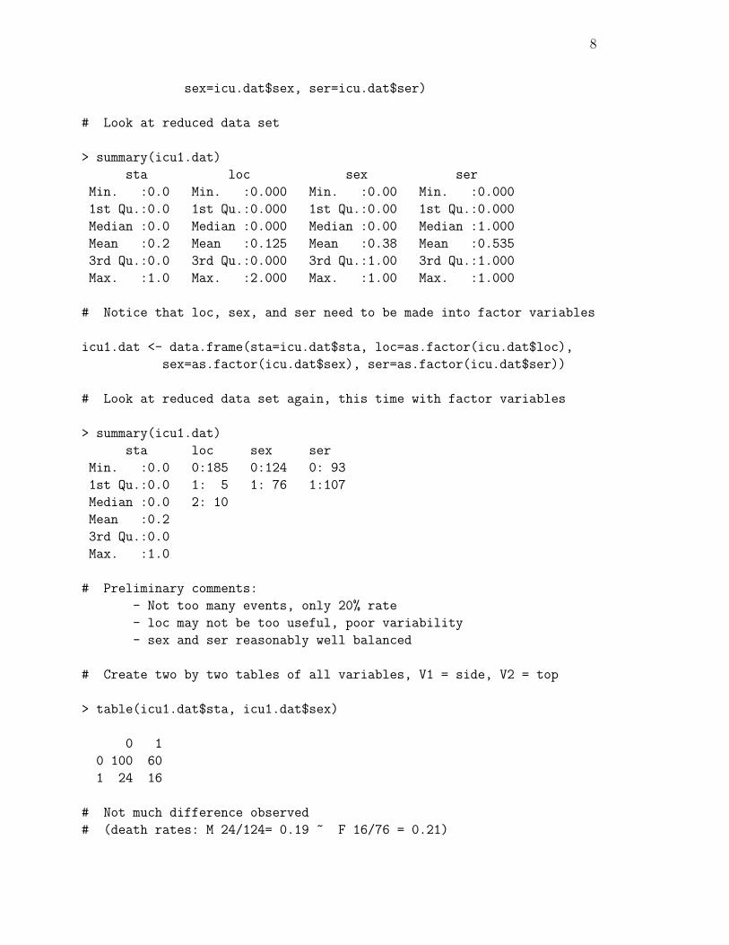
# Look at reduced data set
> summary(icu1.dat)
sta loc sex ser
Min. :0.0 Min. :0.000 Min. :0.00 Min. :0.000
1st Qu.:0.0 1st Qu.:0.000 1st Qu.:0.00 1st Qu.:0.000
Median :0.0 Median :0.000 Median :0.00 Median :1.000
Mean :0.2 Mean :0.125 Mean :0.38 Mean :0.535
3rd Qu.:0.0 3rd Qu.:0.000 3rd Qu.:1.00 3rd Qu.:1.000
Max. :1.0 Max. :2.000 Max. :1.00 Max. :1.000
# Notice that loc, sex, and ser need to be made into factor variables
icu1.dat <- data.frame(sta=icu.dat$sta, loc=as.factor(icu.dat$loc),
sex=as.factor(icu.dat$sex), ser=as.factor(icu.dat$ser))
# Look at reduced data set again, this time with factor variables
> summary(icu1.dat)
sta loc sex ser
Min. :0.0 0:185 0:124 0: 93
1st Qu.:0.0 1: 5 1: 76 1:107
Median :0.0 2: 10
Mean :0.2
3rd Qu.:0.0
Max. :1.0
# Preliminary comments:
- Not too many events, only 20% rate
- loc may not be too useful, poor variability
- sex and ser reasonably well balanced
# Create two by two tables of all variables, V1 = side, V2 = top
> table(icu1.dat$sta, icu1.dat$sex)
0 1
0 100 60
1 24 16
# Not much difference observed
# (death rates: M 24/124= 0.19 ~ F 16/76 = 0.21)

9
> table(icu1.dat$sta, icu1.dat$ser)
0 1
0 67 93
1 26 14
# Fewer deaths (sta=1) at the surgical unit (ser=1),
# OR = 67*14/(26*93) = 0.39
> table(icu1.dat$sta, icu1.dat$loc)
0 1 2
0 158 0 2
1 27 5 8
# Probably very low accuracy here,
# but many more deaths in cats 1 and 2.
> table(icu1.dat$sex, icu1.dat$ser)
0 1
0 54 70
1 39 37
# A bit, but not too much potential for confounding here,
# especially since effect of sex is not strong to begin with
> table(icu1.dat$sex, icu1.dat$loc)
0 1 2
0 116 3 5
1 69 2 5
# Too few data points to say much, maybe females
# have higher values of loc
> table(icu1.dat$ser, icu1.dat$loc)
0 1 2
0 84 2 7
1 101 3 3
# Again hard to say much
# Overall, loc does not look too useful, not much
# effect from any of these variables except maybe for ser.
10
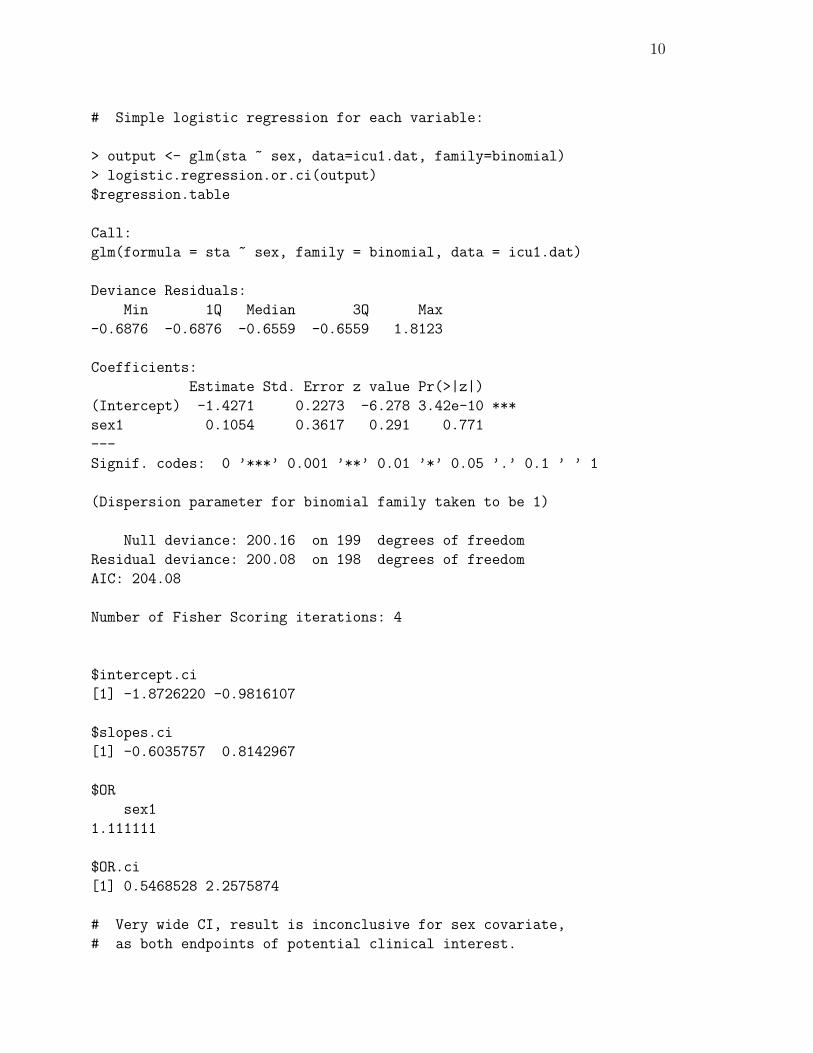
# Simple logistic regression for each variable:
> output <- glm(sta ~ sex, data=icu1.dat, family=binomial)
> logistic.regression.or.ci(output)
$regression.table
Call:
glm(formula = sta ~ sex, family = binomial, data = icu1.dat)
Deviance Residuals:
Min 1Q Median 3Q Max
-0.6876 -0.6876 -0.6559 -0.6559 1.8123
Coefficients:
Estimate Std. Error z value Pr(>|z|)
(Intercept) -1.4271 0.2273 -6.278 3.42e-10 ***
sex1 0.1054 0.3617 0.291 0.771
---
Signif. codes: 0 ’***’ 0.001 ’**’ 0.01 ’*’ 0.05 ’.’ 0.1 ’ ’ 1
(Dispersion parameter for binomial family taken to be 1)
Null deviance: 200.16 on 199 degrees of freedom
Residual deviance: 200.08 on 198 degrees of freedom
AIC: 204.08
Number of Fisher Scoring iterations: 4
$intercept.ci
[1] -1.8726220 -0.9816107
$slopes.ci
[1] -0.6035757 0.8142967
$OR
sex1
1.111111
$OR.ci
[1] 0.5468528 2.2575874
# Very wide CI, result is inconclusive for sex covariate,
# as both endpoints of potential clinical interest.
11
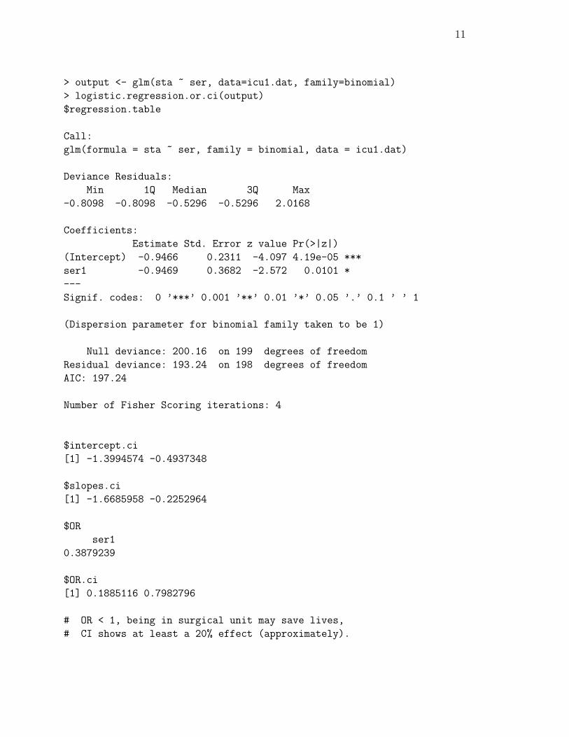
> output <- glm(sta ~ ser, data=icu1.dat, family=binomial)
> logistic.regression.or.ci(output)
$regression.table
Call:
glm(formula = sta ~ ser, family = binomial, data = icu1.dat)
Deviance Residuals:
Min 1Q Median 3Q Max
-0.8098 -0.8098 -0.5296 -0.5296 2.0168
Coefficients:
Estimate Std. Error z value Pr(>|z|)
(Intercept) -0.9466 0.2311 -4.097 4.19e-05 ***
ser1 -0.9469 0.3682 -2.572 0.0101 *
---
Signif. codes: 0 ’***’ 0.001 ’**’ 0.01 ’*’ 0.05 ’.’ 0.1 ’ ’ 1
(Dispersion parameter for binomial family taken to be 1)
Null deviance: 200.16 on 199 degrees of freedom
Residual deviance: 193.24 on 198 degrees of freedom
AIC: 197.24
Number of Fisher Scoring iterations: 4
$intercept.ci
[1] -1.3994574 -0.4937348
$slopes.ci
[1] -1.6685958 -0.2252964
$OR
ser1
0.3879239
$OR.ci
[1] 0.1885116 0.7982796
# OR < 1, being in surgical unit may save lives,
# CI shows at least a 20% effect (approximately).
12
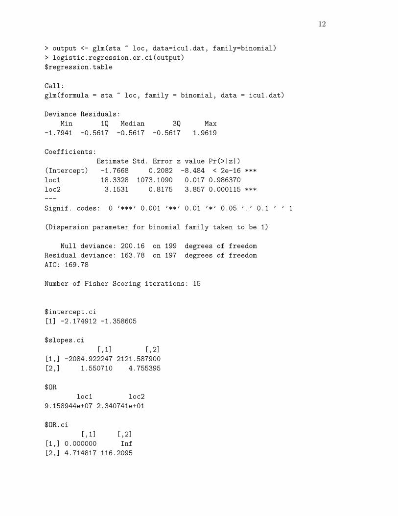
> output <- glm(sta ~ loc, data=icu1.dat, family=binomial)
> logistic.regression.or.ci(output)
$regression.table
Call:
glm(formula = sta ~ loc, family = binomial, data = icu1.dat)
Deviance Residuals:
Min 1Q Median 3Q Max
-1.7941 -0.5617 -0.5617 -0.5617 1.9619
Coefficients:
Estimate Std. Error z value Pr(>|z|)
(Intercept) -1.7668 0.2082 -8.484 < 2e-16 ***
loc1 18.3328 1073.1090 0.017 0.986370
loc2 3.1531 0.8175 3.857 0.000115 ***
---
Signif. codes: 0 ’***’ 0.001 ’**’ 0.01 ’*’ 0.05 ’.’ 0.1 ’ ’ 1
(Dispersion parameter for binomial family taken to be 1)
Null deviance: 200.16 on 199 degrees of freedom
Residual deviance: 163.78 on 197 degrees of freedom
AIC: 169.78
Number of Fisher Scoring iterations: 15
$intercept.ci
[1] -2.174912 -1.358605
$slopes.ci
[,1] [,2]
[1,] -2084.922247 2121.587900
[2,] 1.550710 4.755395
$OR
loc1 loc2
9.158944e+07 2.340741e+01
$OR.ci
[,1] [,2]
[1,] 0.000000 Inf
[2,] 4.714817 116.2095
13
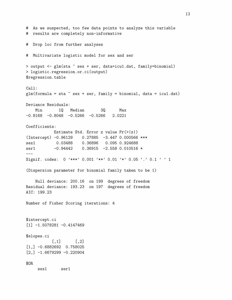
# As we suspected, too few data points to analyze this variable
# results are completely non-informative
# Drop loc from further analyses
# Multivariate logistic model for sex and ser
> output <- glm(sta ~ sex + ser, data=icu1.dat, family=binomial)
> logistic.regression.or.ci(output)
$regression.table
Call:
glm(formula = sta ~ sex + ser, family = binomial, data = icu1.dat)
Deviance Residuals:
Min 1Q Median 3Q Max
-0.8168 -0.8048 -0.5266 -0.5266 2.0221
Coefficients:
Estimate Std. Error z value Pr(>|z|)
(Intercept) -0.96129 0.27885 -3.447 0.000566 ***
sex1 0.03488 0.36896 0.095 0.924688
ser1 -0.94442 0.36915 -2.558 0.010516 *
---
Signif. codes: 0 ’***’ 0.001 ’**’ 0.01 ’*’ 0.05 ’.’ 0.1 ’ ’ 1
(Dispersion parameter for binomial family taken to be 1)
Null deviance: 200.16 on 199 degrees of freedom
Residual deviance: 193.23 on 197 degrees of freedom
AIC: 199.23
Number of Fisher Scoring iterations: 4
$intercept.ci
[1] -1.5078281 -0.4147469
$slopes.ci
[,1] [,2]
[1,] -0.6882692 0.758025
[2,] -1.6679299 -0.220904
$OR
sex1 ser1
14
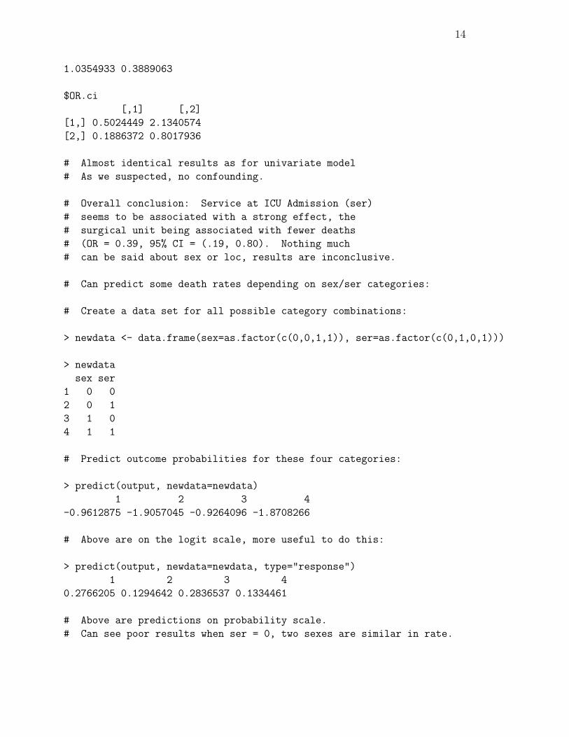
1.0354933 0.3889063
$OR.ci
[,1] [,2]
[1,] 0.5024449 2.1340574
[2,] 0.1886372 0.8017936
# Almost identical results as for univariate model
# As we suspected, no confounding.
# Overall conclusion: Service at ICU Admission (ser)
# seems to be associated with a strong effect, the
# surgical unit being associated with fewer deaths
# (OR = 0.39, 95% CI = (.19, 0.80). Nothing much
# can be said about sex or loc, results are inconclusive.
# Can predict some death rates depending on sex/ser categories:
# Create a data set for all possible category combinations:
> newdata <- data.frame(sex=as.factor(c(0,0,1,1)), ser=as.factor(c(0,1,0,1)))
> newdata
sex ser
1 0 0
2 0 1
3 1 0
4 1 1
# Predict outcome probabilities for these four categories:
> predict(output, newdata=newdata)
1 2 3 4
-0.9612875 -1.9057045 -0.9264096 -1.8708266
# Above are on the logit scale, more useful to do this:
> predict(output, newdata=newdata, type="response")
1 2 3 4
0.2766205 0.1294642 0.2836537 0.1334461
# Above are predictions on probability scale.
# Can see poor results when ser = 0, two sexes are similar in rate.
15
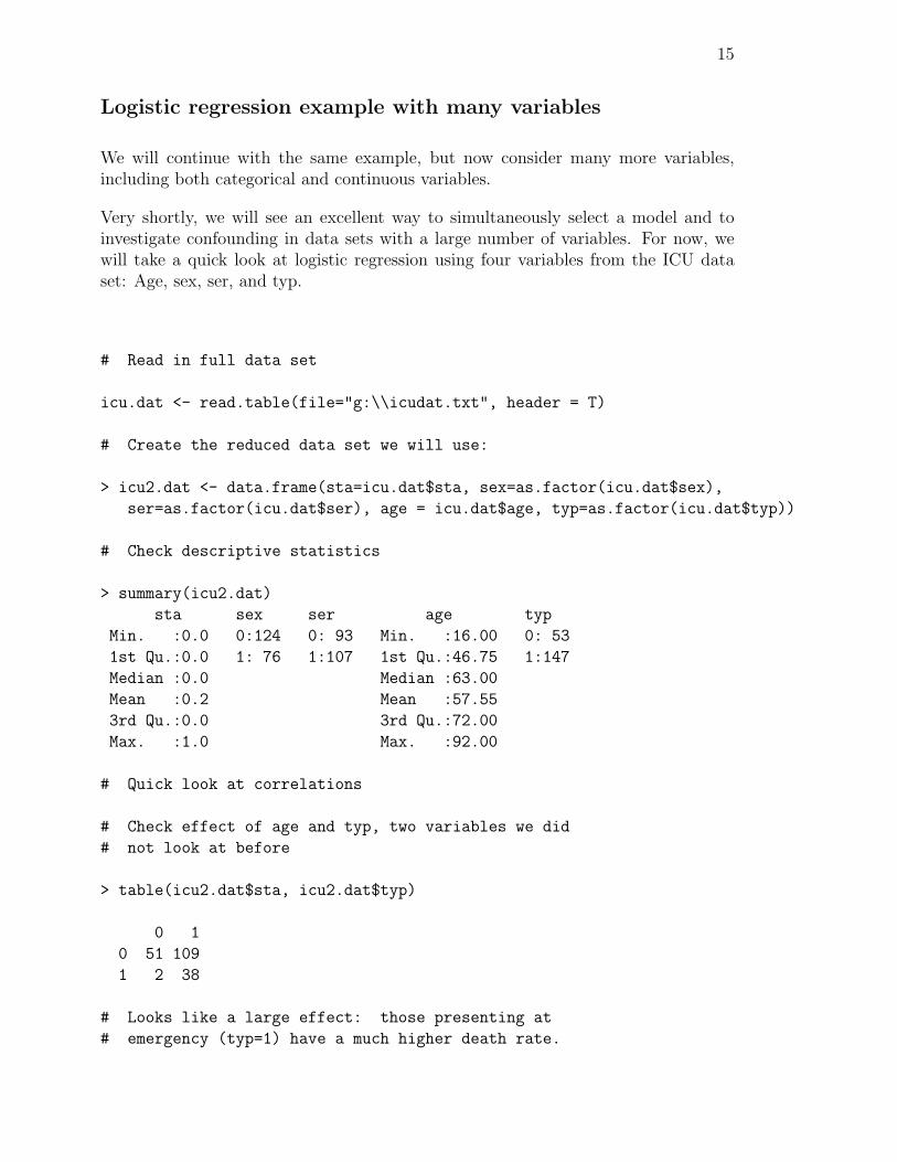
Logistic regression example with many variables
We will continue with the same example, but now consider many more variables,including both categorical and continuous variables.
Very shortly, we will see an excellent way to simultaneously select a model and toinvestigate confounding in data sets with a large number of variables. For now, wewill take a quick look at logistic regression using four variables from the ICU dataset: Age, sex, ser, and typ.
# Read in full data set
icu.dat <- read.table(file="g:\\icudat.txt", header = T)
# Create the reduced data set we will use:
> icu2.dat <- data.frame(sta=icu.dat$sta, sex=as.factor(icu.dat$sex),
ser=as.factor(icu.dat$ser), age = icu.dat$age, typ=as.factor(icu.dat$typ))
# Check descriptive statistics
> summary(icu2.dat)
sta sex ser age typ
Min. :0.0 0:124 0: 93 Min. :16.00 0: 53
1st Qu.:0.0 1: 76 1:107 1st Qu.:46.75 1:147
Median :0.0 Median :63.00
Mean :0.2 Mean :57.55
3rd Qu.:0.0 3rd Qu.:72.00
Max. :1.0 Max. :92.00
# Quick look at correlations
# Check effect of age and typ, two variables we did
# not look at before
> table(icu2.dat$sta, icu2.dat$typ)
0 1
0 51 109
1 2 38
# Looks like a large effect: those presenting at
# emergency (typ=1) have a much higher death rate.

16
# Let’s also look at a table between ser and typ:
> table(icu2.dat$ser, icu2.dat$typ)
0 1
0 1 92
1 52 55
# Looks like there could be some confounding here,
# these are strongly related.
# Check the association between age and the outcome, sta
> boxplot(list(icu2.dat$age[icu2.dat$sta==0], icu2.dat$age[icu2.dat$sta==1]))
It looks like those with higher ages also have higher death rates.
Let’s look at a regression with all five variables included:
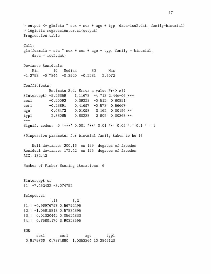
17
> output <- glm(sta ~ sex + ser + age + typ, data=icu2.dat, family=binomial)
> logistic.regression.or.ci(output)
$regression.table
Call:
glm(formula = sta ~ sex + ser + age + typ, family = binomial,
data = icu2.dat)
Deviance Residuals:
Min 1Q Median 3Q Max
-1.2753 -0.7844 -0.3920 -0.2281 2.5072
Coefficients:
Estimate Std. Error z value Pr(>|z|)
(Intercept) -5.26359 1.11678 -4.713 2.44e-06 ***
sex1 -0.20092 0.39228 -0.512 0.60851
ser1 -0.23891 0.41697 -0.573 0.56667
age 0.03473 0.01098 3.162 0.00156 **
typ1 2.33065 0.80238 2.905 0.00368 **
---
Signif. codes: 0 ’***’ 0.001 ’**’ 0.01 ’*’ 0.05 ’.’ 0.1 ’ ’ 1
(Dispersion parameter for binomial family taken to be 1)
Null deviance: 200.16 on 199 degrees of freedom
Residual deviance: 172.42 on 195 degrees of freedom
AIC: 182.42
Number of Fisher Scoring iterations: 6
$intercept.ci
[1] -7.452432 -3.074752
$slopes.ci
[,1] [,2]
[1,] -0.96976797 0.56792495
[2,] -1.05615818 0.57834395
[3,] 0.01320442 0.05624833
[4,] 0.75801170 3.90328595
$OR
sex1 ser1 age typ1
0.8179766 0.7874880 1.0353364 10.2846123

18
$OR.ci
[,1] [,2]
[1,] 0.3791710 1.764602
[2,] 0.3477894 1.783083
[3,] 1.0132920 1.057860
[4,] 2.1340289 49.565050
As expected, age has a strong effect, with an odds ratio of 1.035 per year, or 1.03510 =1.41 per decade (95% CI per year of (1.013, 1.058), so (1.138, 1.757) per decade). Typalso has a very strong effect, with a CI of at least 2.
There does indeed seem to be some confounding between ser and typ, as the coefficientestimate for ser has changed drastically from when typ was not in the model. In fact,ser no longer looks “important”, it has been “replaced” by typ. Because of the highcorrelation between ser and typ, it is difficult to separate out the effects of these twovariables.
We will return to this issue when we discuss model selection for logistic regression.
Logistic regression with interaction terms
Going back to the example where we had just sex and ser in the model, what if wewanted to investigate an interaction term between these two variables?
So far, we have seen that ser is associated with a strong effect, but the effect of sexwas inconclusive. But, what if the effect of ser is different among males and females,i.e., what if we have an interaction (or sometimes called effect modification) betweensex and ser?
Here is how to investigate this for logistic regression in R:
# Create the variable that will be used in the interaction:
# Create a blank vector to store new variable
> ser.sex <- rep(0, length(icu1.dat$ser))
# Change value to 1 when both ser and sex are one
> for (i in 1:length(icu1.dat$ser)) {if (icu1.dat$ser[i] == 1
& icu1.dat$sex[i] == 1) ser.sex[i] <- 1 }
# Check new variable
19
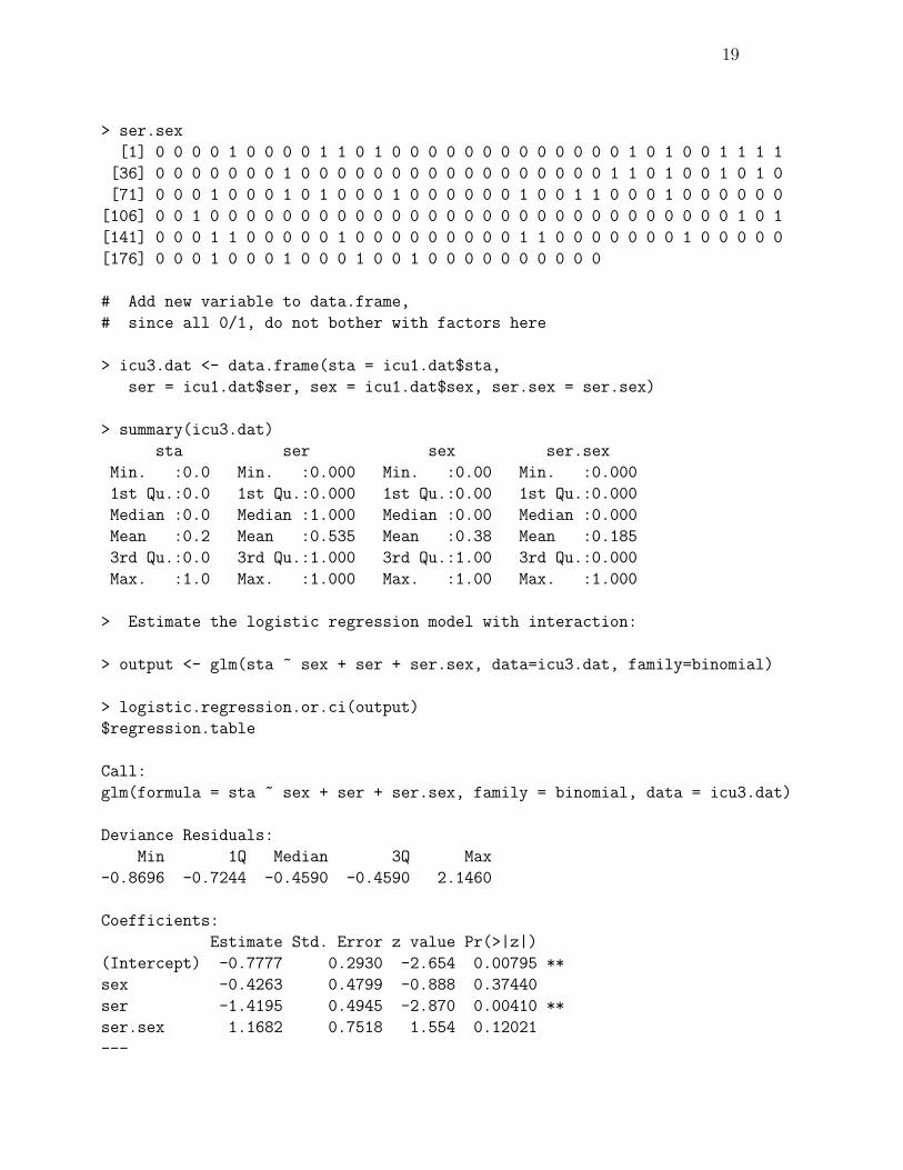
> ser.sex
[1] 0 0 0 0 1 0 0 0 0 1 1 0 1 0 0 0 0 0 0 0 0 0 0 0 0 0 1 0 1 0 0 1 1 1 1
[36] 0 0 0 0 0 0 0 1 0 0 0 0 0 0 0 0 0 0 0 0 0 0 0 0 0 1 1 0 1 0 0 1 0 1 0
[71] 0 0 0 1 0 0 0 1 0 1 0 0 0 1 0 0 0 0 0 0 1 0 0 1 1 0 0 0 1 0 0 0 0 0 0
[106] 0 0 1 0 0 0 0 0 0 0 0 0 0 0 0 0 0 0 0 0 0 0 0 0 0 0 0 0 0 0 0 0 1 0 1
[141] 0 0 0 1 1 0 0 0 0 0 1 0 0 0 0 0 0 0 0 0 1 1 0 0 0 0 0 0 0 1 0 0 0 0 0
[176] 0 0 0 1 0 0 0 1 0 0 0 1 0 0 1 0 0 0 0 0 0 0 0 0 0
# Add new variable to data.frame,
# since all 0/1, do not bother with factors here
> icu3.dat <- data.frame(sta = icu1.dat$sta,
ser = icu1.dat$ser, sex = icu1.dat$sex, ser.sex = ser.sex)
> summary(icu3.dat)
sta ser sex ser.sex
Min. :0.0 Min. :0.000 Min. :0.00 Min. :0.000
1st Qu.:0.0 1st Qu.:0.000 1st Qu.:0.00 1st Qu.:0.000
Median :0.0 Median :1.000 Median :0.00 Median :0.000
Mean :0.2 Mean :0.535 Mean :0.38 Mean :0.185
3rd Qu.:0.0 3rd Qu.:1.000 3rd Qu.:1.00 3rd Qu.:0.000
Max. :1.0 Max. :1.000 Max. :1.00 Max. :1.000
> Estimate the logistic regression model with interaction:
> output <- glm(sta ~ sex + ser + ser.sex, data=icu3.dat, family=binomial)
> logistic.regression.or.ci(output)
$regression.table
Call:
glm(formula = sta ~ sex + ser + ser.sex, family = binomial, data = icu3.dat)
Deviance Residuals:
Min 1Q Median 3Q Max
-0.8696 -0.7244 -0.4590 -0.4590 2.1460
Coefficients:
Estimate Std. Error z value Pr(>|z|)
(Intercept) -0.7777 0.2930 -2.654 0.00795 **
sex -0.4263 0.4799 -0.888 0.37440
ser -1.4195 0.4945 -2.870 0.00410 **
ser.sex 1.1682 0.7518 1.554 0.12021
---
20
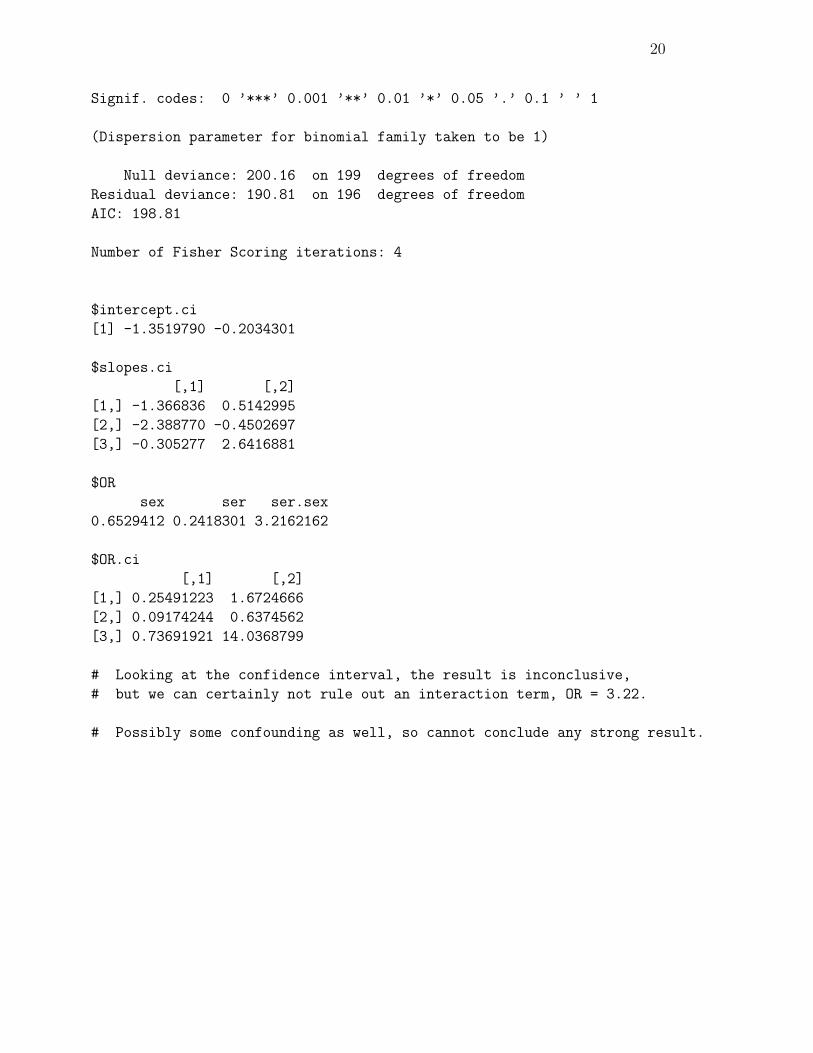
Signif. codes: 0 ’***’ 0.001 ’**’ 0.01 ’*’ 0.05 ’.’ 0.1 ’ ’ 1
(Dispersion parameter for binomial family taken to be 1)
Null deviance: 200.16 on 199 degrees of freedom
Residual deviance: 190.81 on 196 degrees of freedom
AIC: 198.81
Number of Fisher Scoring iterations: 4
$intercept.ci
[1] -1.3519790 -0.2034301
$slopes.ci
[,1] [,2]
[1,] -1.366836 0.5142995
[2,] -2.388770 -0.4502697
[3,] -0.305277 2.6416881
$OR
sex ser ser.sex
0.6529412 0.2418301 3.2162162
$OR.ci
[,1] [,2]
[1,] 0.25491223 1.6724666
[2,] 0.09174244 0.6374562
[3,] 0.73691921 14.0368799
# Looking at the confidence interval, the result is inconclusive,
# but we can certainly not rule out an interaction term, OR = 3.22.
# Possibly some confounding as well, so cannot conclude any strong result.

21
Note on ORs in presence of confounding
Note that one needs to be careful in interpreting the Odds Ratios from the aboveoutputs, because of the interaction term.
The OR given above for the sex variable, 0.653, applies only within the medical service(coded as 0 in the ser variable), and the OR given above for ser, 0.242, applies onlywithin males (coded 0 in the sex variable).
In order to obtain the OR for sex within the ser = 1 (surgical category), or toobtain the OR for ser within females (sex = 1), one need to multiple by the OR fromthe interaction term. Hence, we have:
OR for ser within females = 0.242 * 3.22 = 0.779.
OR for sex within surgical unit = 0.653 * 3.22 = 2.10.