Using Structural Equation Modeling to Analyze Monitoring Data

Jim Grace

NWRC

What is structural equation modeling?

A framework for using statistical methods to ask complex questions of data.

Macrohabitat

ηc1

Microhabitat

ηc2

Diversity

ηe3

Litter

ηe2

Herbaceous

ηe1

lake, x1

impound, x2

swale, x3

vhit1, y1

vhit2, y2

herbl, y3

herbc, y4

wlitr, y5

litrd, y6

litrc, y7

rich, y8

0

0

.26

.75

.98

.92.64

.90

.81 -.47

.95

1.13

.44

ns

ns

1.0 1.0

.80

1.00

.59.77

The Origin of Structural Equation Modeling

Sewell Wright1897-1988

1st paper in:1920

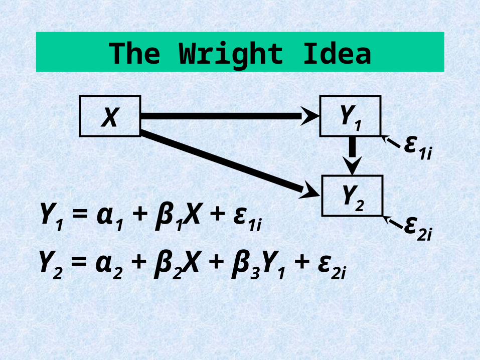
The Wright Idea

Y1 = α1 + β1X + ε1i

Y2 = α2 + β2X + β3Y1 + ε2i

X Y1ε1i

Y2

ε2i

The LISREL Synthesis

Karl Jöreskog1934 - present

Key Synthesis paper- 1973

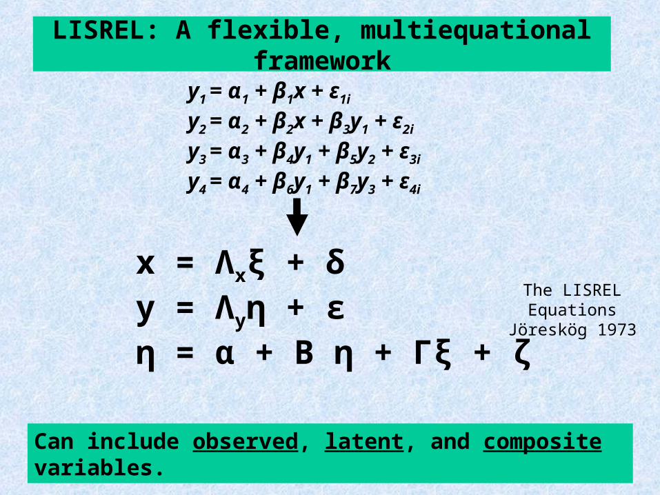
LISREL: A flexible, multiequational framework

y1 = α1 + β1x + ε1i y2 = α2 + β2x + β3y1 + ε2i

y3 = α3 + β4y1 + β5y2 + ε3i

y4 = α4 + β6y1 + β7y3 + ε4i

Can include observed, latent, and composite variables.

x = Λxξ + δy = Λyη + εη = α + Β η + Γξ + ζ

The LISREL Equations

Jöreskög 1973

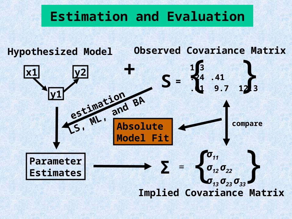
Σ = {σ11

σ12 σ22

σ13 σ23 σ33

}Implied Covariance Matrix

compareAbsolute Model Fit

x1

y1

y2

Hypothesized Model Observed Covariance Matrix

{1.3.24 .41.01 9.7 12.3}S =

+

Estimation and Evaluation

ParameterEstimates

estimation

LS, ML, and BA

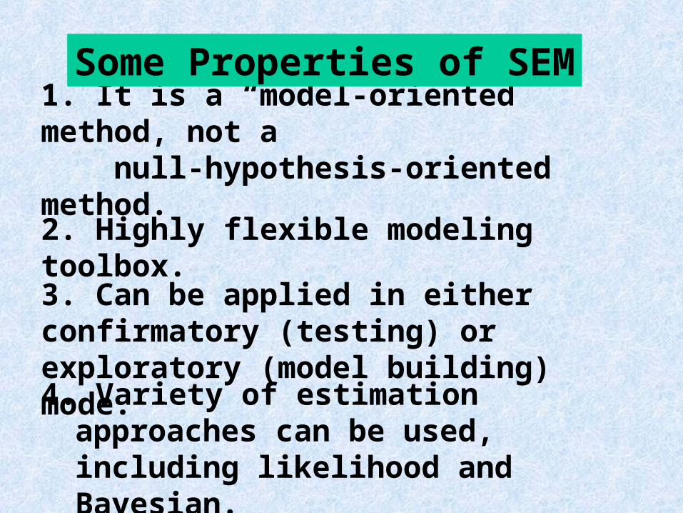
1. It is a “model-oriented” method, not a null-hypothesis-oriented method.

Some Properties of SEM

2. Highly flexible modeling toolbox.

3. Can be applied in either confirmatory (testing) or exploratory (model building) mode.

4. Variety of estimation approaches can be used, including likelihood and Bayesian.

1. Seeks to model uncertainty rather than probabilities.

A Bit about the Bayesian Approach

2. Philosophically well suited for supporting decision making.

3. Popularity partly based on new algorithms that create great flexibility in modeling.

4. It's indeterminant solution procedure, contributes to some uncertainty about results for more complex models(?)

Why do we need multivariate modeling?

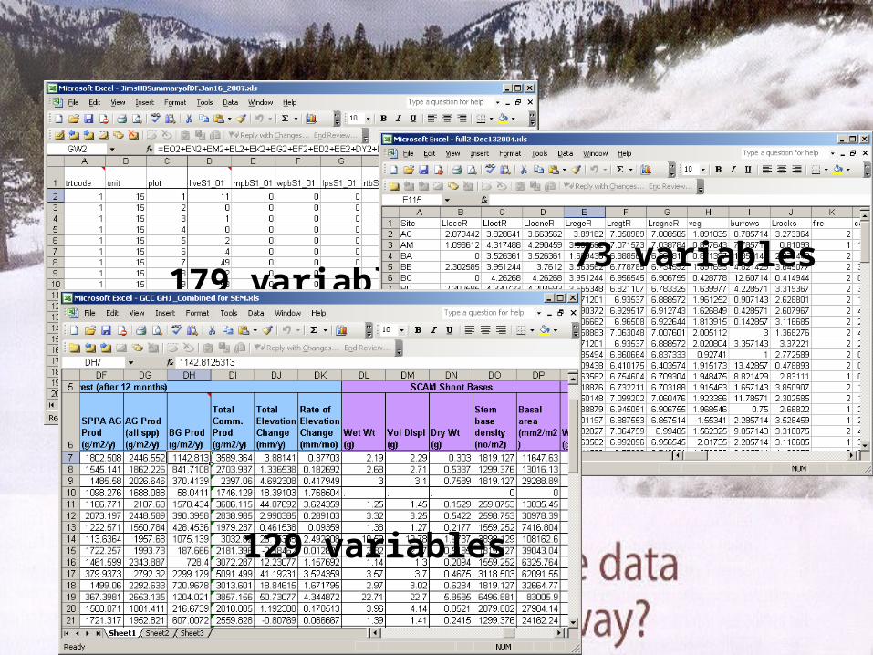
179 variables73 variables

129 variables

Do the conventional methods meet your needs?

All your greatscientific ideas!

ANOVA result you hope to get!

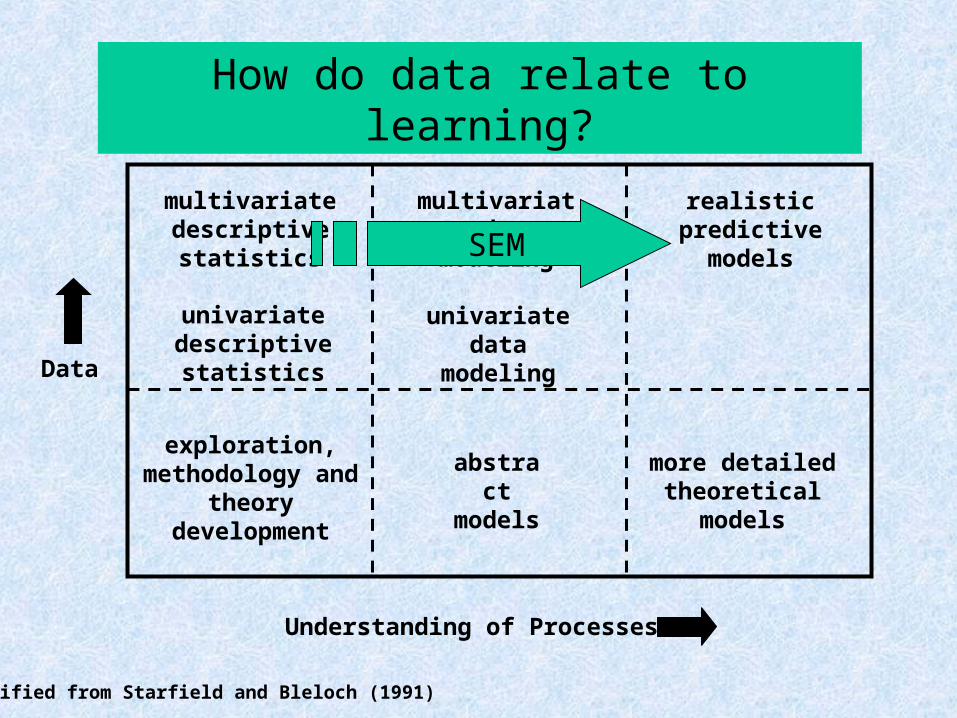
modified from Starfield and Bleloch (1991)

How do data relate to learning?

Understanding of Processes

univariate descriptive statistics

exploration, methodology and

theory development

realistic predictive models

abstract models

multivariate descriptive statistics

more detailed theoretical models

univariate data modeling

multivariate data modeling

Data

SEM

Example #1:Theodore Roosevelt Natl. Park

Weed Problem

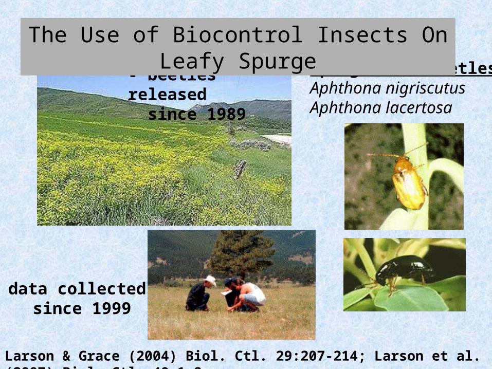
Larson & Grace (2004) Biol. Ctl. 29:207-214; Larson et al. (2007) Biol. Ctl. 40:1-8.

spurge flea beetlesAphthona nigriscutusAphthona lacertosa

- beetles released since 1989

The Use of Biocontrol Insects On Leafy Spurge

- data collected since 1999

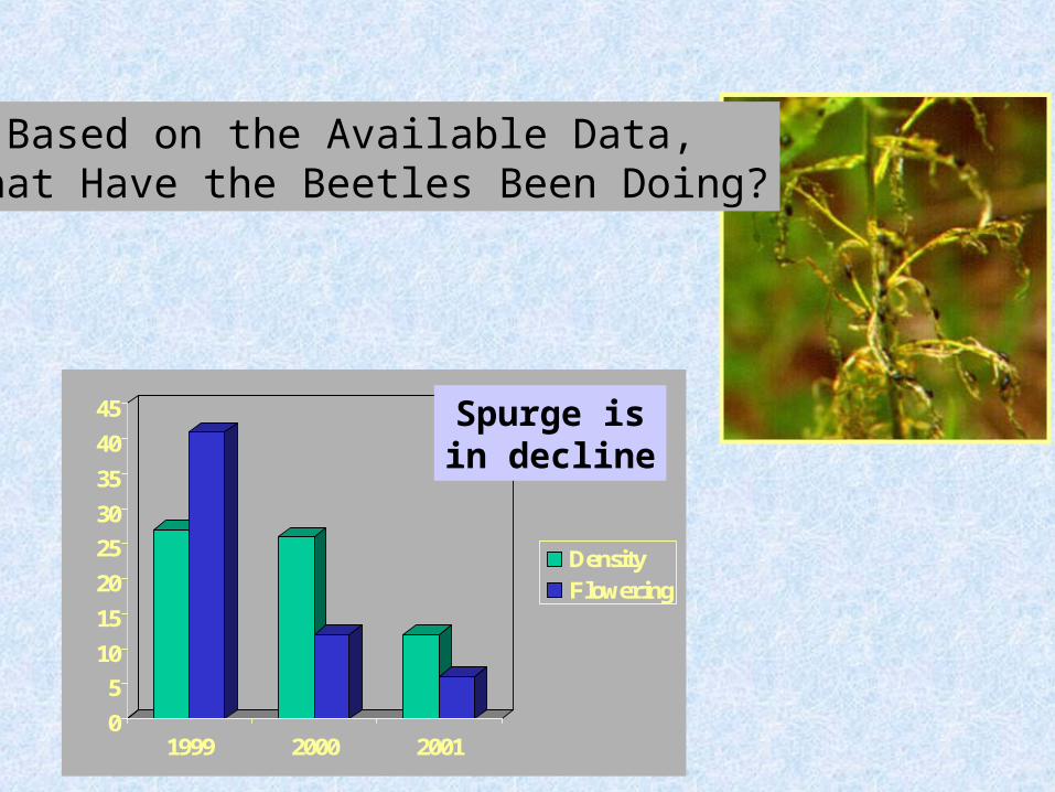
Based on the Available Data, What Have the Beetles Been Doing?

0

5

10

15

20

25

30

35

40

45

1999 2000 2001

DensityFlowering

Spurge isin decline

-100

-80

-60

-40

-20

0

20

40

0 2 4 6

log A. nigriscutis

% C

han

ge i

n S

pu

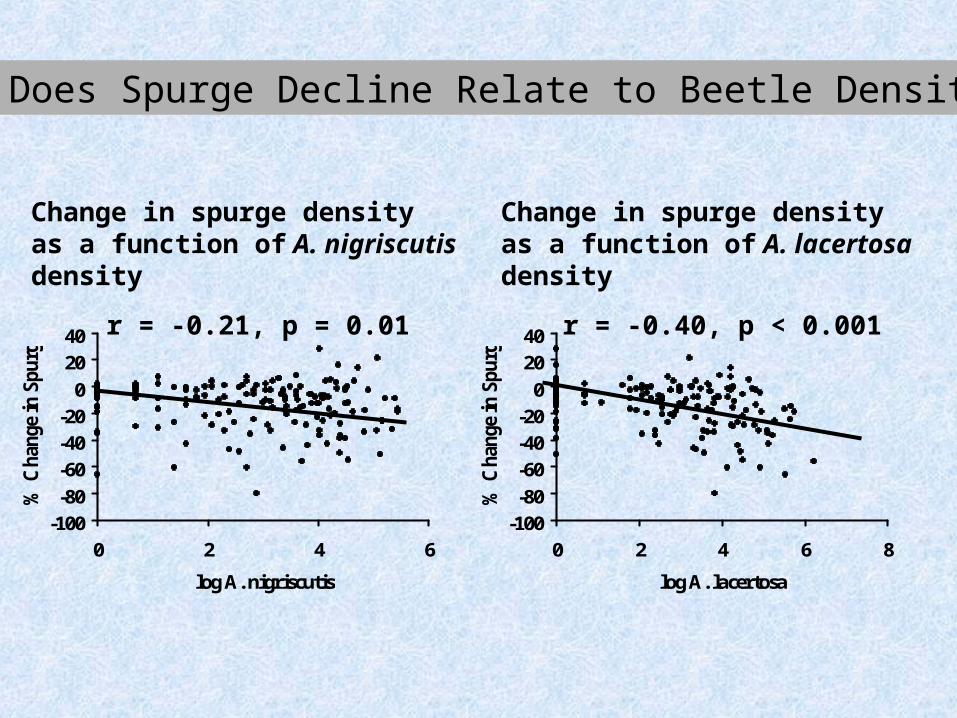
rge r = -0.21, p = 0.01

Change in spurge densityas a function of A. nigriscutisdensity

-100

-80

-60

-40

-20

0

20

40

0 2 4 6 8

log A. lacertosa

% C

han

ge i

n S

pu

rge r = -0.40, p < 0.001

Change in spurge densityas a function of A. lacertosadensity

How Does Spurge Decline Relate to Beetle Density?

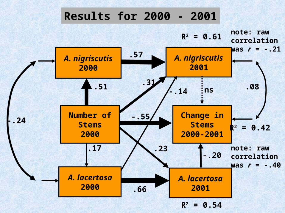
Multivariate View: Hypothesized Model

A. lacertosa2001

Number ofStems2000

A. nigriscutis2000

A. lacertosa2000

A. nigriscutis2001

Change inStems

2000-2001

Change inStems

2000-2001

A. nigriscutis2001

Number ofStems2000

A. nigriscutis2000

A. lacertosa2001

A. lacertosa2000

R2 = 0.54

R2 = 0.61

-.20

.66

.57

.31-.14

-.55

.23

.51

.17

-.24R2 = 0.42

.08

Results for 2000 - 2001note: rawcorrelationwas r = -.21

note: rawcorrelationwas r = -.40

ns

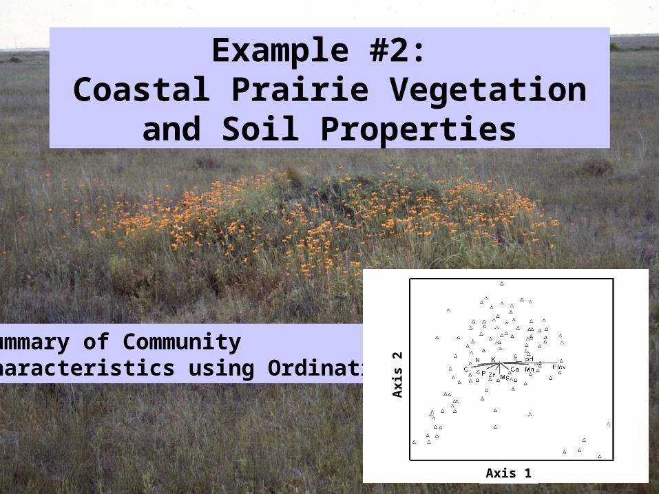
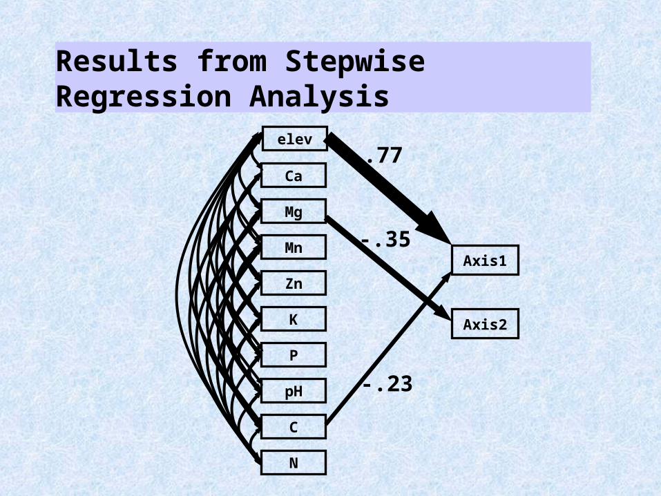
Example #2: Coastal Prairie Vegetation and Soil

Properties

Summary of CommunityCharacteristics using Ordination

Axis 1

Axi

s 2

Mg

Mn

N

Ca

Zn

K

P

pH

C

Axis1

elev

Axis2

.77

-.23

-.35

Results from Stepwise Regression Analysis

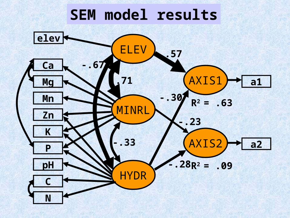
SEM model results

Mg

Mn

N

Ca

Zn

K

P

pH

C

elevELEV

MINRL

HYDR

-.67

.71

-.33 AXIS2

AXIS1

a2

a1

.57

-.30

-.28

-.23

R2 = .63

R2 = .09

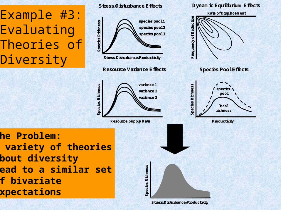
The Problem:A variety of theoriesabout diversitylead to a similar setof bivariate expectations

Stress/Disturbance/Productivity

Sp

ecie

s R

ich

ne

ss

Stress/Disturbance/Productivity

Sp

ecie

s R

ich

ne

ss

Stress/Disturbance Effects

Stress/Disturbance/Productivity

Sp

ec

ies

Ric

hn

ess species pool 1

species pool 2

species pool 3

Stress/Disturbance Effects

Stress/Disturbance/Productivity

Sp

ec

ies

Ric

hn

ess species pool 1

species pool 2

species pool 3

Stress/Disturbance/Productivity

Sp

ec

ies

Ric

hn

ess species pool 1

species pool 2

species pool 3

Dynamic Equilibrium Effects

Rate of Displacement

Fre

qu

en

cy

of

Re

du

cti

on

Dynamic Equilibrium Effects

Rate of Displacement

Fre

qu

en

cy

of

Re

du

cti

on

Resource Variance Effects

Resource Supply Rate

Sp

eci

es

Ric

hn

es

s variance 1

variance 2

variance 3

Resource Variance Effects

Resource Supply Rate

Sp

eci

es

Ric

hn

es

s variance 1

variance 2

variance 3

Species Pool Effects

Productivity

Sp

ec

ies

Ric

hn

es

s

species pool

local richness

Species Pool Effects

Productivity

Sp

ec

ies

Ric

hn

es

s

species pool

local richness

Example #3:EvaluatingTheories ofDiversity

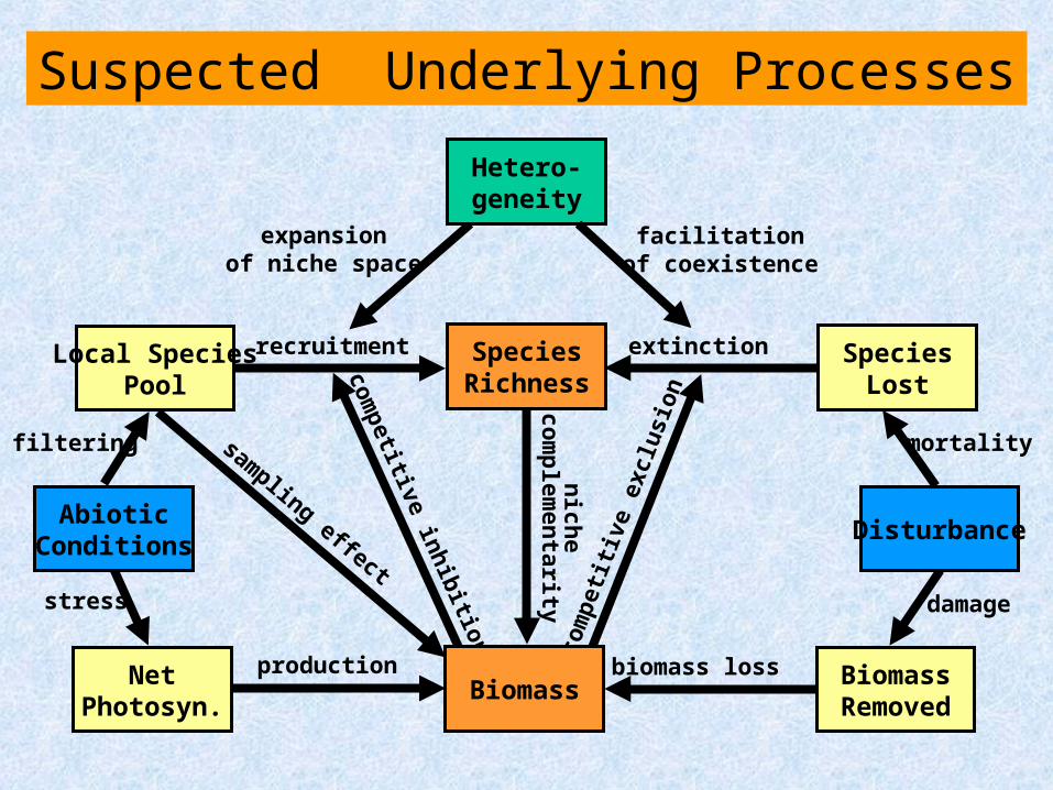
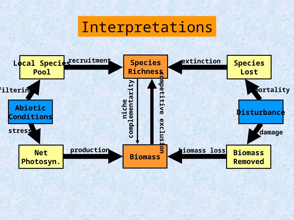
Suspected Underlying Processes

com

peti

tive

exc

lusi

oncom

petitive inhibition

sampling effect

AbioticConditions

stress

filtering

Hetero-geneity

facilitationof coexistence

expansionof niche space

Disturbance

damage

mortality

recruitment extinctionSpeciesRichness

SpeciesLost

Local SpeciesPool

Biomassproduction biomass loss Biomass

RemovedNet

Photosyn.

nich

ecom

plem

entarity

National Center for Ecological Analysis and Synthesis Project

Finnish meadows

Kansas prairie

Louisiana prairie

Minn. prairie

Texas grasslands

Louisiana marsh2

Indian tropicalsavanna

Louisiana marsh1

Wisconsin prairie

Miss. prairie

Utah grassland

Africa grassland

AbioticConditions

stress

filtering

Disturbance

damage

mortality

recruitment extinctionSpeciesRichness

SpeciesLost

Local SpeciesPool

Biomassproduction biomass loss Biomass

RemovedNet

Photosyn.

Interpretations

nic

he

com

ple

men

tari

tycom

petitive exclu

sion

Collaborative Applications of Multivariate Modeling

• USGS - Numerous units and individuals

• Univ. California - Davis

• Univ. Northern Arizona

• Univ. North Carolina

• Univ. Alabama

• Univ. Minnesota

• Nat. Ctr. Ecol. Analysis

• Univ. New Mexico

• Purdue Univ.

• Univ. Texas - Arlington

• Michigan State Univ.

• Univ. Groenegen (The Netherlands)

• Syracuse Univ.

• Rice Univ.

• Univ. Houston

• LSU

• US Forest Service

• Colorado State Univ.

• Univ. California - Irving

• Oregon State Univ.

• Yale Univ.

• Univ. Wisc. - Eau Claire

• Univ. Connecticut

• Univ. Newcastle - UK

• Univ. Montpellier - France