Performance analysis of an operational implementation of WRF

Todd HutchinsonWSI Corporation

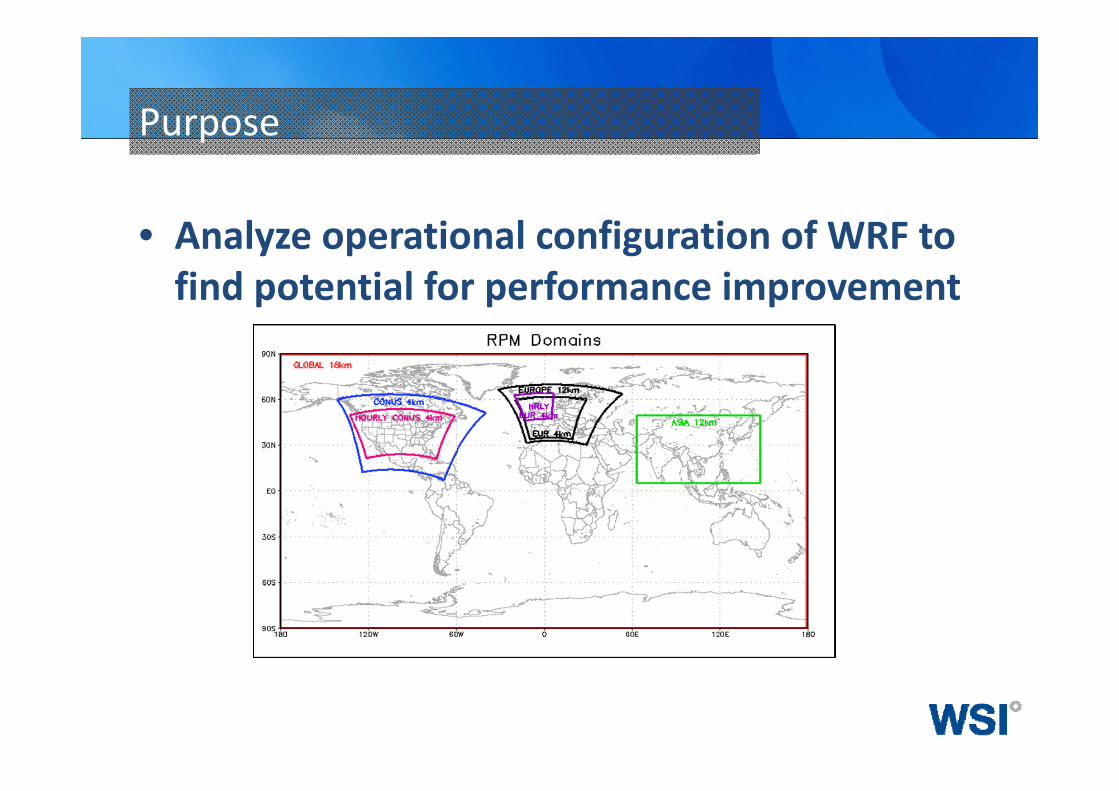
Purpose

• Analyze operational configuration of WRF to find potential for performance improvement

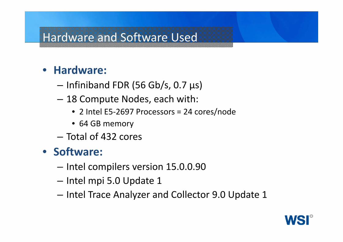
Hardware and Software Used

• Hardware:– Infiniband FDR (56 Gb/s, 0.7 μs)– 18 Compute Nodes, each with:

• 2 Intel E5‐2697 Processors = 24 cores/node• 64 GB memory

– Total of 432 cores• Software:

– Intel compilers version 15.0.0.90– Intel mpi 5.0 Update 1– Intel Trace Analyzer and Collector 9.0 Update 1

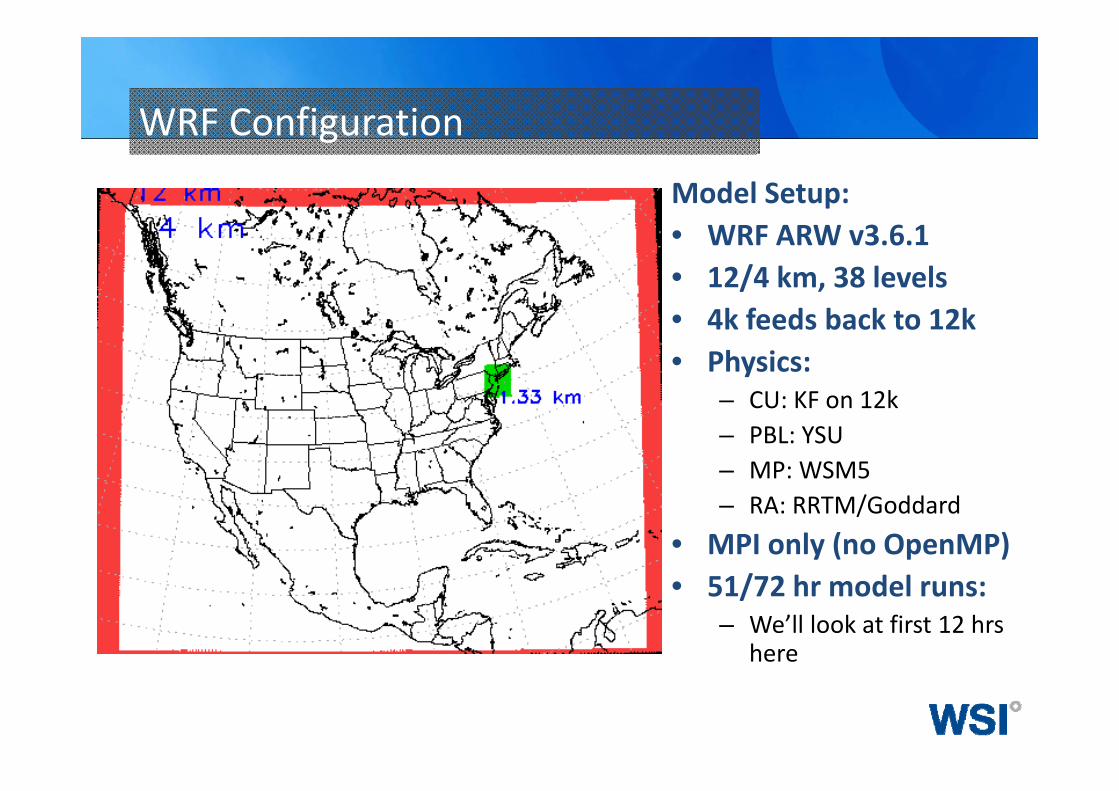
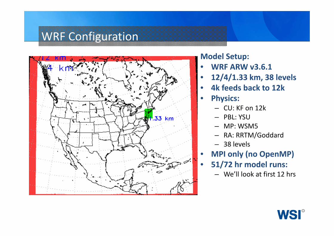
WRF Configuration

Model Setup:• WRF ARW v3.6.1• 12/4 km, 38 levels• 4k feeds back to 12k• Physics:

– CU: KF on 12k– PBL: YSU– MP: WSM5– RA: RRTM/Goddard

• MPI only (no OpenMP)• 51/72 hr model runs:

– We’ll look at first 12 hrshere

0

0.05

0.1

0.15

0.2

0.25

0.3

0.35

Time Spent (s) in Each Function

Slowest Rank

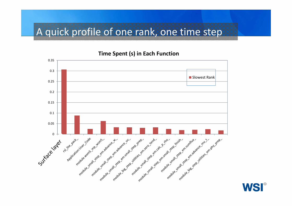
A quick profile of one rank, one time step

The profile reveals:

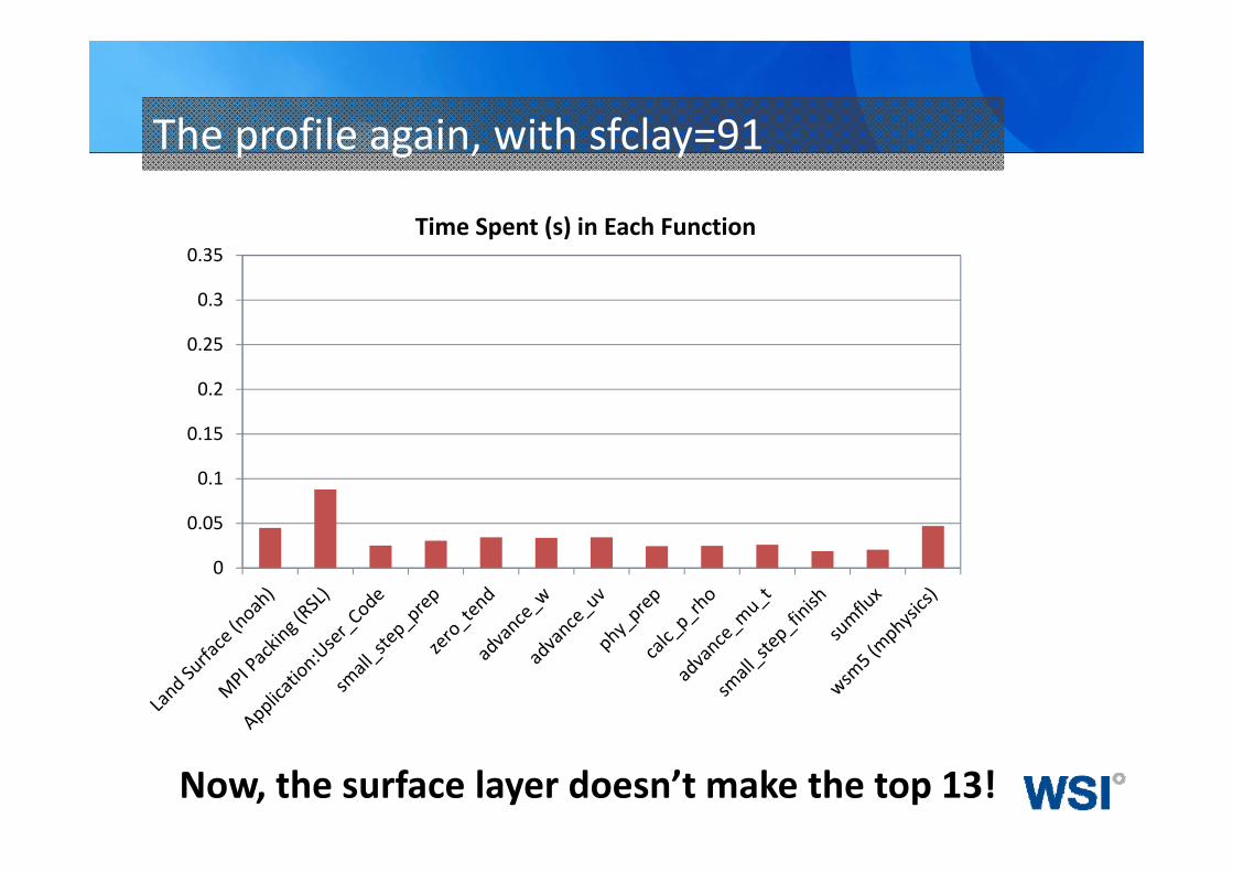
• The surface layer calculation (sf_sfclay=1) is taking up 40% of the run time!

• Further analysis showed that this was an issue introduced in WRF3.6

• WRF Developers at NCAR are investigating• The quick fix is to set sf_sfclay=91 (the older version of this surface layer scheme)

0

0.05

0.1

0.15

0.2

0.25

0.3

0.35Time Spent (s) in Each Function

The profile again, with sfclay=91

Now, the surface layer doesn’t make the top 13!

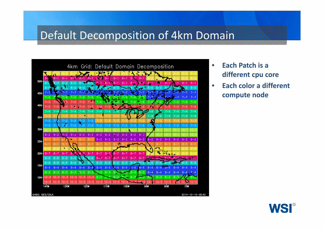
Default Decomposition of 4km Domain

• Each Patch is a different cpu core

• Each color a different compute node

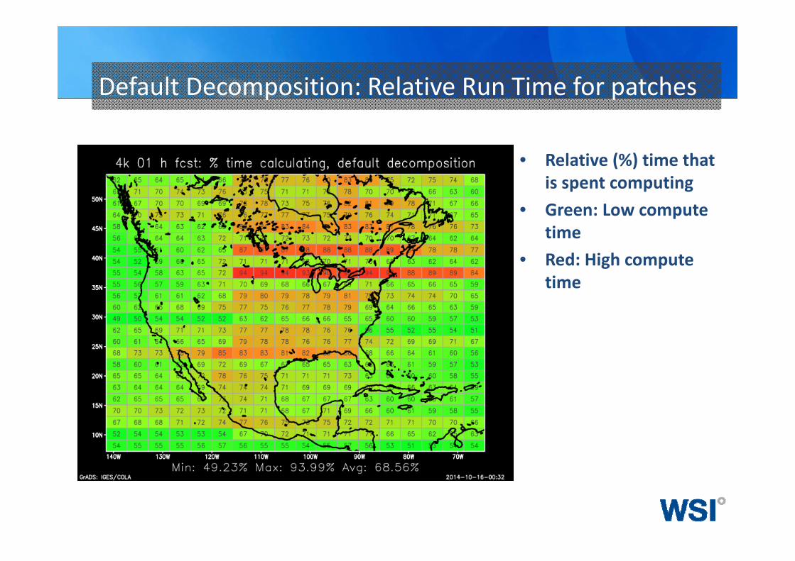
Default Decomposition: Relative Run Time for patches 

• Relative (%) time that is spent computing

• Green: Low compute time

• Red: High compute time

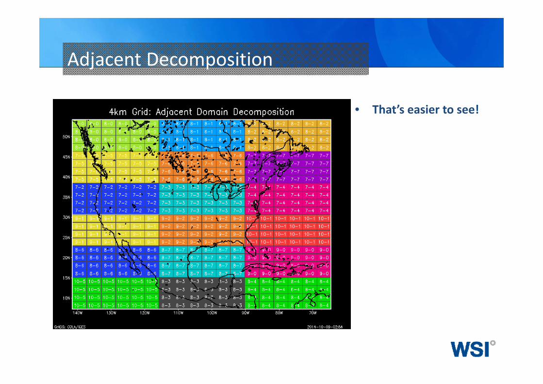
Adjacent Decomposition

• That’s easier to see!

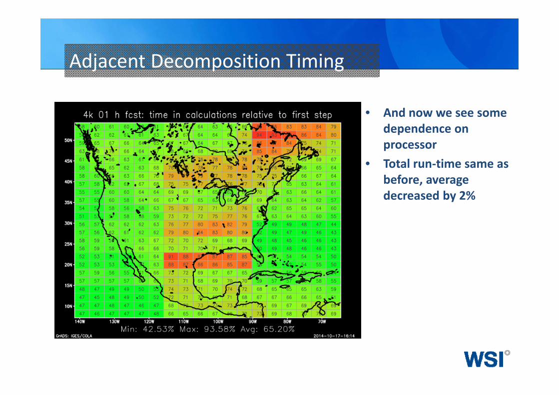
Adjacent Decomposition Timing

• And now we see some dependence on processor

• Total run‐time same as before, average decreased by 2%

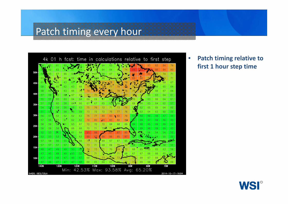
Patch timing every hour

• Patch timing relative to first 1 hour step time

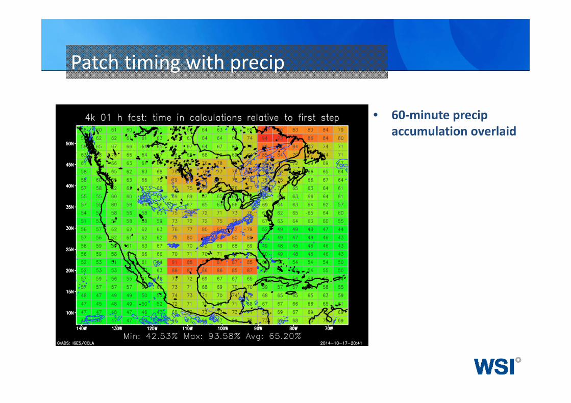
Patch timing with precip

• 60‐minute precipaccumulation overlaid

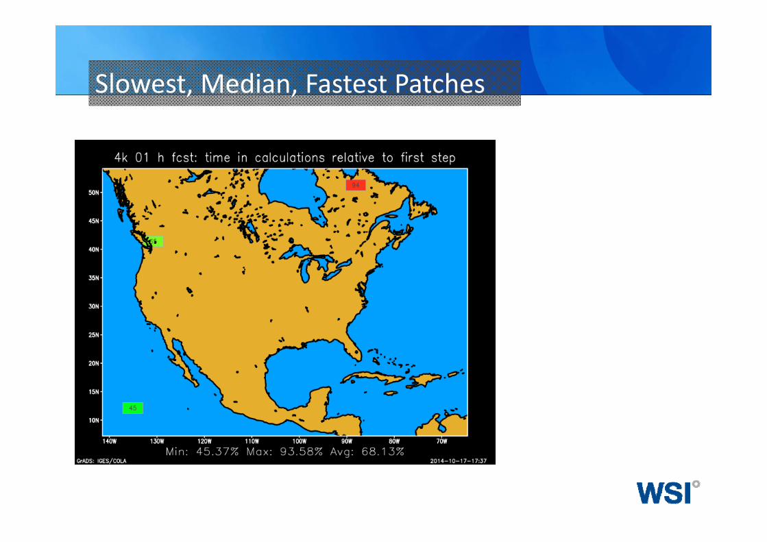
Slowest, Median, Fastest Patches

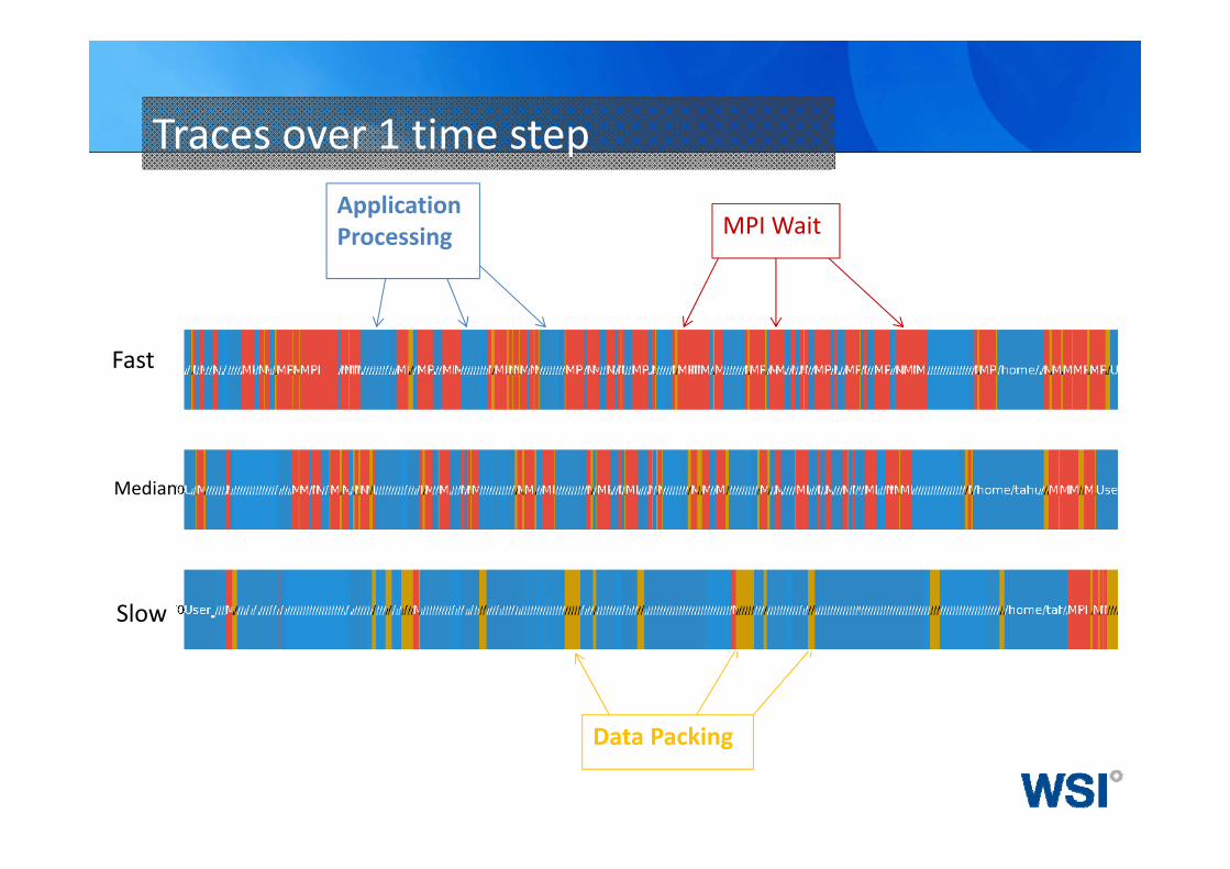
Traces over 1 time step

Fast

Median

Slow

Application Processing MPI Wait

Data Packing

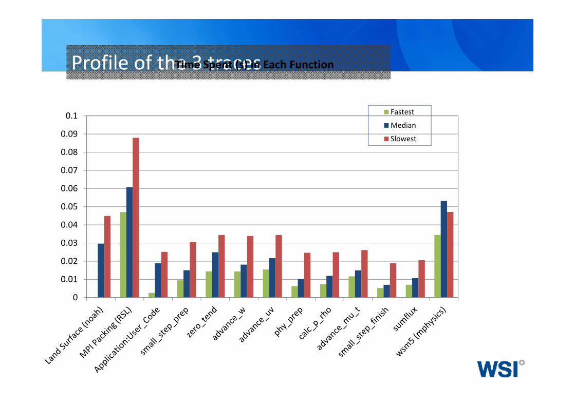
Profile of the 3 traces

0

0.01

0.02

0.03

0.04

0.05

0.06

0.07

0.08

0.09

0.1

Time Spent (s) in Each Function

Fastest

Median

Slowest

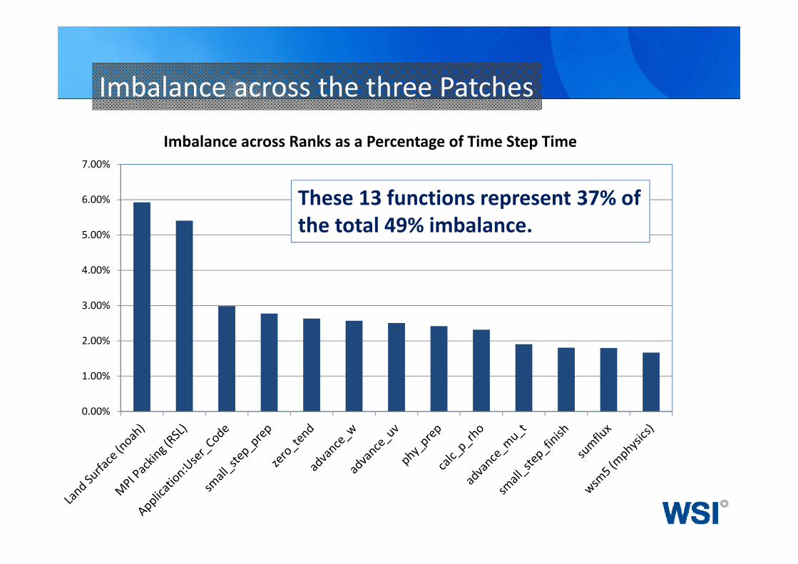
Imbalance across the three Patches

0.00%

1.00%

2.00%

3.00%

4.00%

5.00%

6.00%

7.00%

Imbalance across Ranks as a Percentage of Time Step Time

These 13 functions represent 37% of the total 49% imbalance. 

WRF ConfigurationModel Setup:• WRF ARW v3.6.1• 12/4/1.33 km, 38 levels• 4k feeds back to 12k• Physics:

– CU: KF on 12k– PBL: YSU– MP: WSM5– RA: RRTM/Goddard– 38 levels

• MPI only (no OpenMP)• 51/72 hr model runs:

– We’ll look at first 12 hrs

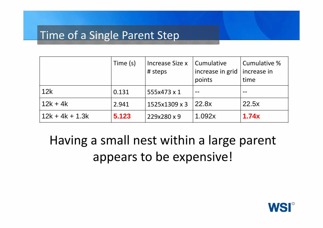
Time of a Single Parent Step

Time (s) Increase Size x # steps

Cumulativeincrease in grid points

Cumulative % increase in time

12k 0.131 555x473 x 1 -- --

12k + 4k 2.941 1525x1309 x 3 22.8x 22.5x

12k + 4k + 1.3k 5.123 229x280 x 9 1.092x 1.74x

Having a small nest within a large parent appears to be expensive!

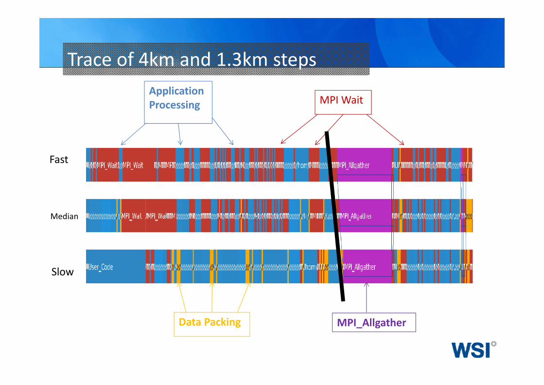
Trace of 4km and 1.3km steps

Fast

Median

Slow

Application Processing MPI Wait

Data Packing MPI_Allgather

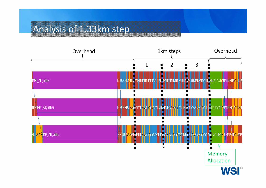
Analysis of 1.33km step

1km steps

1                 2                 3 

Overhead Overhead

Memory Allocation

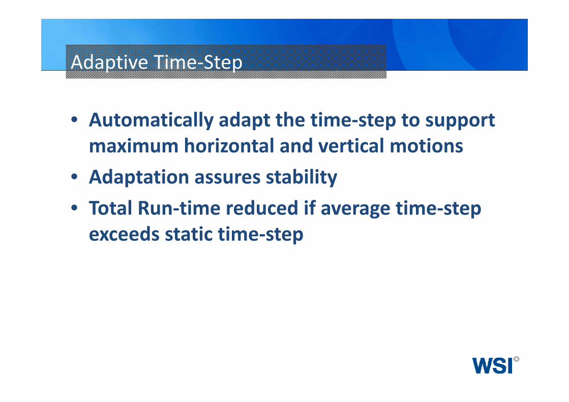
Adaptive Time‐Step

• Automatically adapt the time‐step to support maximum horizontal and vertical motions

• Adaptation assures stability• Total Run‐time reduced if average time‐step exceeds static time‐step

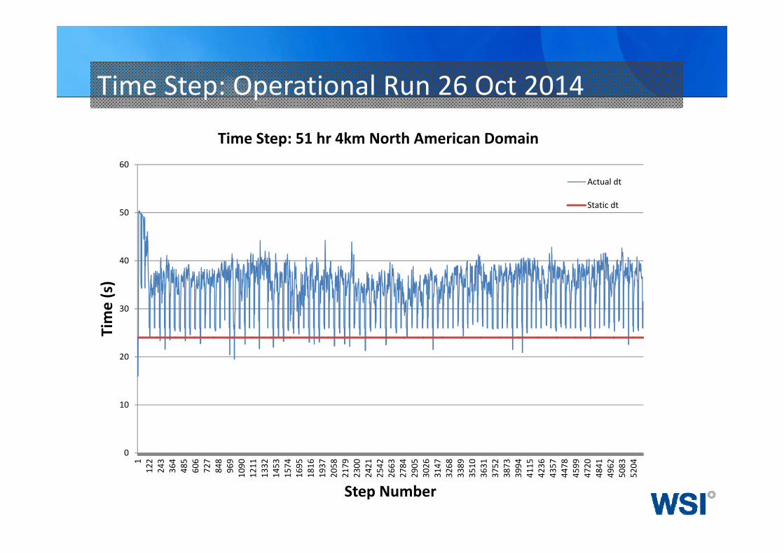
Time Step: Operational Run 26 Oct 2014

0

10

20

30

40

50

60

1122

243

364

485

606

727

848

969

1090

1211

1332

1453

1574

1695

1816

1937

2058

2179

2300

2421

2542

2663

2784

2905

3026

3147

3268

3389

3510

3631

3752

3873

3994

4115

4236

4357

4478

4599

4720

4841

4962

5083

5204

Time (s)

Step Number

Time Step: 51 hr 4km North American Domain

Actual dt

Static dt

Run Time

Feb               Mar                    Apr                 May                   Jun                     Jul                Aug                    Sep

0

50

100

150

200

2501 39 77 115

153

191

229

267

305

343

381

419

457

495

533

571

609

647

685

723

761

799

837

875

913

951

989

1027

1065

1103

1141

1179

1217

1255

1293

1331

1369

1407

1445

1483

1521

1559

1597

1635

1673

1711

Run Time (m

in)

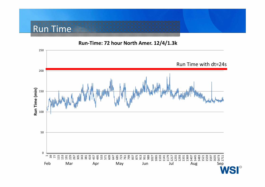
Run‐Time: 72 hour North Amer. 12/4/1.3k 

Run Time with dt=24s

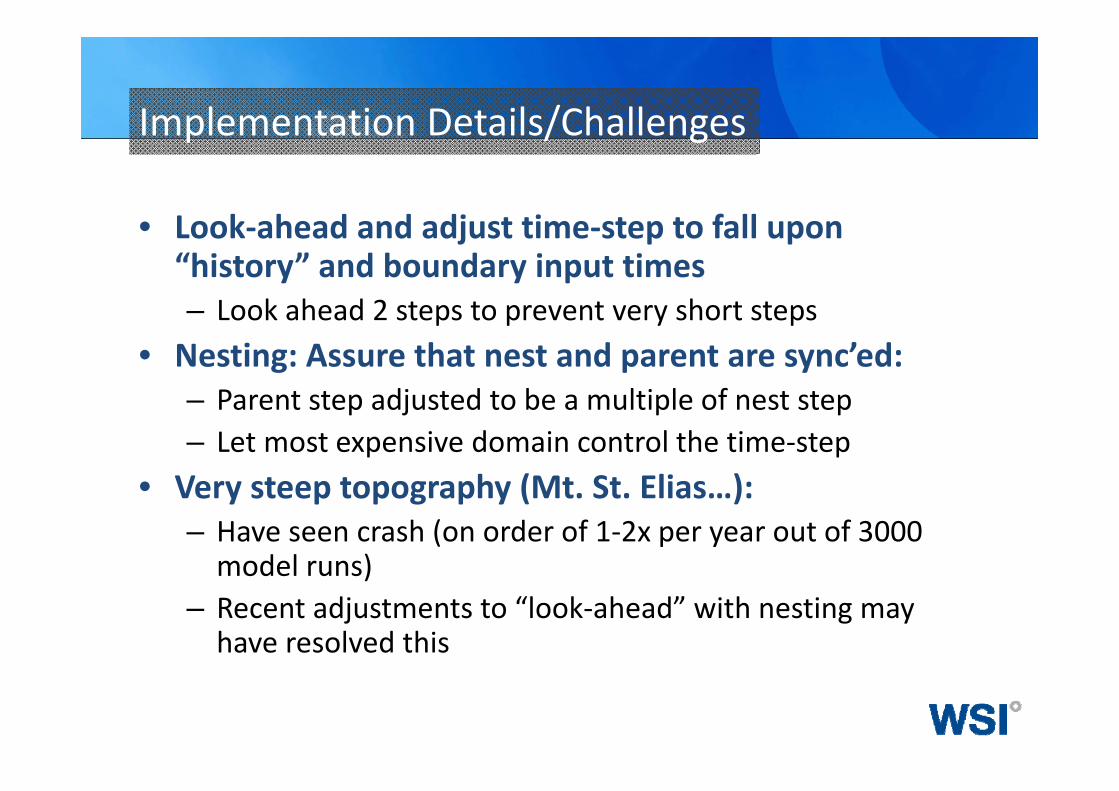
Implementation Details/Challenges

• Look‐ahead and adjust time‐step to fall upon “history” and boundary input times– Look ahead 2 steps to prevent very short steps

• Nesting: Assure that nest and parent are sync’ed:– Parent step adjusted to be a multiple of nest step– Let most expensive domain control the time‐step

• Very steep topography (Mt. St. Elias…):– Have seen crash (on order of 1‐2x per year out of 3000 model runs)

– Recent adjustments to “look‐ahead” with nesting may have resolved this

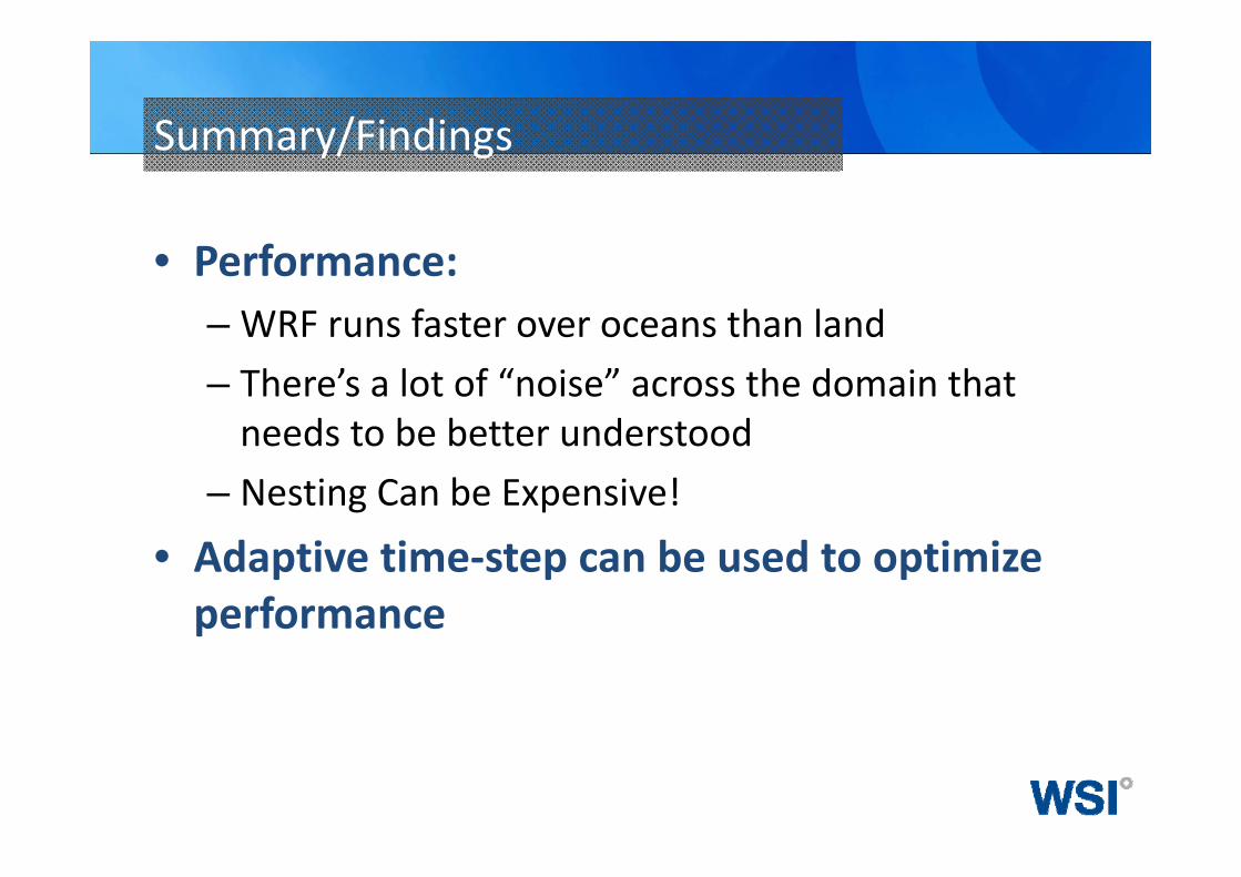
Summary/Findings

• Performance:– WRF runs faster over oceans than land– There’s a lot of “noise” across the domain that needs to be better understood

– Nesting Can be Expensive!

• Adaptive time‐step can be used to optimize performance