Top k Knapsack Joins - Paris Dauphine Universitylitwin/Top k Knapsack Join and Closure8.pdfTop k...
17
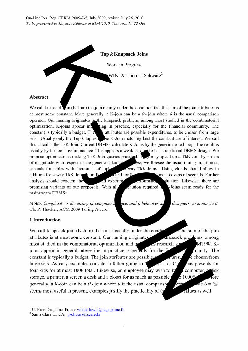
1 Top k Knapsack Joins Work in Progress Witold LITWIN 1 & Thomas Schwarz 2 Abstract We call knapsack join (K-Join) the join mainly under the condition that the sum of the join attributes is at most some constant. More generally, a K-join can be a θ - join where θ is the usual comparison operator. Our naming originates in the knapsack problem, among most studied in the combinatorial optimization. K-joins appear interesting in practice, especially for the financial community. The constant is typically a budget. The join attributes are possible expenditures, to be chosen from large sets. Usually only the Top k tuples of the K-Join matching best the constant are of interest. We call this calculus the TkK-Join. Current DBMSs calculate K-Joins by the generic nested loop. The result is usually by far too slow in practice. This appears a weakness in the basic relational DBMS design. We propose optimizations making TkK-Join queries practical. They may speed-up a TkK-Join by orders of magnitude with respect to the generic calculus. In finale, we foresee the usual timing in, at most, seconds for tables with thousands of tuples and 6-way TkK-Joins. Using clouds should allow in addition for 4-way TkK-Joins in milliseconds and for 8–way TkK-Joins in dozens of seconds. Further analysis should concern the formal and experimental performance evaluation. Likewise, there are promising variants of our proposals. With all the caution required TkK-Joins seem ready for the mainstream DBMSs. Motto. Complexity is the enemy of computer science, and it behooves us, as designers, to minimize it. Ch. P. Thacker, ACM 2009 Turing Award. 1.Introduction We call knapsack join (K-Join) the join basically under the condition that the sum of the join attributes is at most some constant. Our naming originates in the knapsack problems, among most studied in the combinatorial optimization and operations research generally /MT90/. K- joins appear in general interesting in practice, especially for the financial community. The constant is typically a budget. The join attributes are possible expenditures, to be chosen from large sets. As easy examples consider a father going to ToysRUs for Christmas presents for four kids for at most 100€ total. Likewise, an employee may wish to buy a computer, a disk storage, a printer, a screen a desk and a closet for as much as possible up to 1000€ total. More generally, a K-join can be a θ - join where θ is the usual comparison operator. While θ = ‘≤’ seems most useful at present, examples justify the practicality of the other θ-values as well. 1 U. Paris Dauphine, France [email protected] 2 Santa Clara U., CA, [email protected] On-Line Res. Rep. CERIA 2009-7-5, July 2009, revised July 26, 2010 To be presented as Keynote Address at BDA’2010, Toulouse 19-22 Oct. K - jOIN
Transcript of Top k Knapsack Joins - Paris Dauphine Universitylitwin/Top k Knapsack Join and Closure8.pdfTop k...
1
Top k Knapsack Joins
Work in Progress
Witold LITWIN1 & Thomas Schwarz2
Abstract
We call knapsack join (K-Join) the join mainly under the condition that the sum of the join attributes is at most some constant. More generally, a K-join can be a θ - join where θ is the usual comparison operator. Our naming originates in the knapsack problem, among most studied in the combinatorial optimization. K-joins appear interesting in practice, especially for the financial community. The constant is typically a budget. The join attributes are possible expenditures, to be chosen from large sets. Usually only the Top k tuples of the K-Join matching best the constant are of interest. We call this calculus the TkK-Join. Current DBMSs calculate K-Joins by the generic nested loop. The result is usually by far too slow in practice. This appears a weakness in the basic relational DBMS design. We propose optimizations making TkK-Join queries practical. They may speed-up a TkK-Join by orders of magnitude with respect to the generic calculus. In finale, we foresee the usual timing in, at most, seconds for tables with thousands of tuples and 6-way TkK-Joins. Using clouds should allow in addition for 4-way TkK-Joins in milliseconds and for 8–way TkK-Joins in dozens of seconds. Further analysis should concern the formal and experimental performance evaluation. Likewise, there are promising variants of our proposals. With all the caution required TkK-Joins seem ready for the mainstream DBMSs.
Motto. Complexity is the enemy of computer science, and it behooves us, as designers, to minimize it. Ch. P. Thacker, ACM 2009 Turing Award.
1.Introduction
We call knapsack join (K-Join) the join basically under the condition that the sum of the join attributes is at most some constant. Our naming originates in the knapsack problems, among most studied in the combinatorial optimization and operations research generally /MT90/. K-joins appear in general interesting in practice, especially for the financial community. The constant is typically a budget. The join attributes are possible expenditures, to be chosen from large sets. As easy examples consider a father going to ToysRUs for Christmas presents for four kids for at most 100€ total. Likewise, an employee may wish to buy a computer, a disk storage, a printer, a screen a desk and a closet for as much as possible up to 1000€ total. More generally, a K-join can be a θ - join where θ is the usual comparison operator. While θ = ‘≤’ seems most useful at present, examples justify the practicality of the other θ-values as well.
1 U. Paris Dauphine, France [email protected] 2 Santa Clara U., CA, [email protected]
On-Line Res. Rep. CERIA 2009-7-5, July 2009, revised July 26, 2010 To be presented as Keynote Address at BDA’2010, Toulouse 19-22 Oct. K - jO
IN

2
Usually, only the Top k tuples of the K-Join matching best the constant are of interest. We call this calculus the TkK-Join. Current DBMSs calculate K-Joins by the generic nested loop. The result is usually by far too slow for the practical use or simply clogs any RDBMS. This appears a weakness in the basic relational DBMS design. We propose optimizations making TkK-Join queries practical. We investigate the improvements to the basic methods for join calculus, i.e., the nested loop, the sort-merge and the join indexes. We also consider the cloud computing.
We show that our proposals may speed-up a TkK-Join by orders of magnitude with respect to the generic nested loop. In finale, we foresee the usual timing in seconds at most for tables with thousands of tuples and 6-way TkK-Joins. Using clouds should allow for 4-way TkK-Joins in milliseconds and for 8–way TkK-Joins in dozens of seconds. With all the caution required our results show TkK-Joins ready for the implementation in mainstream DBMSs.
Section 2 discusses the concept of K-join in detail. It also relates it to the knapsack problems in the combinatorial optimization and operations research. Section 3 presents our optimizations. Section 4 concludes the analysis and points towards the future work. It should focus on further analysis of the formal and experimental evaluation of our proposals. The diversity of the knapsack problems inspires also promising variants and generalizations of our proposals.
2.K-Joins 2.1 Motivating example
Consider the father aiming at four Christmas gifts within its limited budget of 100€. He goes to ToysRUs and asks for help. The choice should be under and as close as possible to his budget limit, e.g., 100€. He also wishes four different toys for variety. ToysRUs has the database with table Toys, with each toy with some Price. As any honest father, ours is definitively not interested by cheap stuff. The helpful query could be then simply as follows:
(1) Select TOP 1 * from Toys T1, Toys T2, Toys T3, Toys T4
Where T1.Price + T2.Price + T3.Price + T4.Price ≤ 100
and T1.Id < T2.Id and T2.Id < T3.Id and T3.Id < T4.Id
Order by T1.Price + T2.Price + T3.Price + T4.Price Desc;
We consider here that Top works without ties, e.g. as for Sql Server, and not as for, e.g., MsAccess. Consider now that Toys has 16K toys (perhaps more in practice). A generic execution of (1) would require the calculus of the Cartesian product of 16K ^ 4 = 256 = 16P tuples. This is enough to clog the largest computers beyond any reasonable waiting time.
In particular, first tests with the well-known Northwind database of Microdoft on the 1GHz Wintel notebook, by the way, using the OrderDetails table with 2K tuples, simply stopped the MsAccess for only binary addition over the UnitPrice attributs. Same test for the only 77-tuple Product table lead to already almost 10s for only 3-value addition. The 4-value query like (1) required 1m40s, often prohibitive in practice.
K - jOIN
3
There are obviously many variants of this example and many similar ones, as above hinted. We postpone the discussion of some to Section 2.x. The above one, understandable to anyone, suffices we believe as the basis.
2.2 Formal Definition of Top k KJoin
One can see the where clause of query (1) as a specific 4-way join. We express indeed usually a join in the relational algebra or in FROM clause of SQL, e.g., an equijoin of two tables R1 and R2 on attributes a1 and a2 (prices, costs, constraints…) as:
(2) R1 Join R2 on a1 = a2
Our operation expresses similarly as:
(3) R1 Join R2 on a1 + a2 ≤ C.
Here, C is some positive constant, C = 100€ in our example. The domains of a1 and of a2 are supposed to be also the positive real values. We do not see the application of the remaining values at present. The syntax (3) is, by the way, legal for FROM clause of a modern DBMS, e.g., MsAccess or SQL Server. As we said, on the other hand, our join condition is a specific, database oriented, version of the combinatorial problem well-known as knapsack problems (KP), /MT90/, /W9/. We recall KP below. For both reasons, we call (3) knapsack join and K-Join in short. We call K-query any query with a K-Join.
The condition (3) defines a 2-way K-Join. More generally, we define the m-way K-Join where m ≥ 2, over m join attributes R1.a1+…Rmam, naturally as follows through SQL-like formalism:
(4) Select * from R1…Rm where R1.a1+…Rmam ≤ C
Here the join attributes are also supposed the positive real values only, although (4) would apply to all the real values as well. However, for the former, 2-way K-joins are associative. One may calculate an m-way K join as the sequence of (m-1) 2-way K-joins, e.g., as follows:
(5) R1 Join (R2 Join… (Rm-1Join Rm on am-1 + am ≤ C) … on a1+ (a2 +…+am) ≤ C
Property (5) may be useful for the join indices, as we show later. As for the usual joins, we can talk furthermore more generally about K-Joins with the comparison operator θ that is as usual θ ∈ {=, <, >, ≤, ≥, =, <>}. The m-way K-join becomes then defined as:
(6) Select * from R1…Rm where R1.a1+…Rmam θ C
Notice that the associativity does not generalize to all the θ values. The analysis of the values of θ other than “≤” is left for the future, although we give examples of their use below. The need for them seems less frequent at this time.
The example shows also that only a few tuples among all those produced by a K-Join would be usually of interest. These are k ≥ 1 tuples matching best the limit C. We can determine these tuples using the usual Top k operator over the dynamic (virtual) attribute R1.a1+…Rmam. The table should be ordered on this attribute in the descending order for θ = ‘≤’ or θ = ‘<’
K - jOIN
4
and in the ascending one or without order for the others. We call the related join TkK-Join. The TkK-Join query is naturally the query with such joins. Sometimes we talk specifically about T1K-Join. In what follows, we limit our attention to queries with TkK-Joins only. The self K-join over table R may provide useless duplicates over permutations of the join values R.a, e.g., (R.a1, R.a2, R.a3) and (R.a3, R.a2, R.a1). For self TkK-Joins we are therefore only interested in the results without such duplicates, eliminated through an additional restriction like in our motivating query (1). Unlike in (1) however, the restriction may allow R.a values to be duplicated in resulting tuples, provided there are no above discussed duplicates. Technically, we do not only allow for the strong either ‘<‘ or ‘>’ inequalities in the additional restriction, but, more generally, for the weak ‘<=’ or ‘>=’ ones.
As usual for joins, one may execute first the restrictions and projections involving join attributes in a K-query. Notice nevertheless that the results of a K-Join and of TkK-join depend not only on the joined relations, but also on C, obviously.
2.3 Knapsack Problems
The Knapsack Problem (KP) is an NP-hard optimization problem among most studied. It can be defined as follows /W9/, /PRP9/. The input is (1) a set O of objects {o1,...on} and (2) an m-d subspace called knapsack K, with bi representing the i-th dimension's capacity of the knapsack, 1 ≤ i ≤ m. The knapsack's constraints matrix with entries we denote ai,j ; 1 ≤ j ≤ n ; stores the constraint values for each object j in each dimension i (price, size, volume...). Then, an output is a set O' of objects stored in the knapsack. Classically, the binary variable xj ; xj ∈ {0, 1}, called 0–1 decision variable, indicates the selection of the object j into the knapsack (x j= 1) or whether it remains out (xj = 0). The vector cj represents further the benefit of the object oj in the knapsack. We select the elements of O’ so that we maximize the total profit of the selected objects, while we match the knapsack constraints, i.e., we maximize:
subject to:
The most frequently investigated case is the 1-d one, i.e. that of i = 1. Often, or perhaps even the most often, the KP concept designates implicitly this case. Frequently, in addition, one also sets every cj to cj = aj. In the combinatorial optimization world, one calls this sub-problem the subset-sum KP. Both conditions are ours below, unless we state otherwise. The case of m > 1, of basic KP and of subset-sum variant, is naturally referred to as multidimensional (MKP). A variant of recent interest of the latter is called quadratic MKP, /QST9/. The case of θ = ‘=’ is known as change-making KP. There can be also several “knapsacks”: what becomes the multiple KP(s). Also, xi may denote the quantity of the object
K - jOIN
5
oi to consider in the above equations, in which case one talks about the unbounded KP, /VKB10/.
For some dimension p > 1, every cj may, on the other hand, be a p-dimensional vector itself. This leads to the so-called, at least 0-1, multi-objective KP, (MOKP), where one especially searches for some or every result not dominated (on all the dimensions) by any other, /BHV9/. Although /BHV9/ does not point it out, MOKP appears a variant of the well-known skyline computation, already advocated for the databases. The specific assumption is that every object candidate for the skyline is in fact the set of the original items matching together the 1-d K constraint. Finally, look, e.g., into /MT90/ for more on the countless KP variations. The general research orientation for KP and MKP was, to our best knowledge, that of a heuristic providing acceptable result for the possibly largest data set in the fastest or acceptable time at least, given necessary constraints on the computer system used. This is in fact, again to our best knowledge, the typical approach of the combinatorial optimization research to NP-hard problems. See, /MT90/, /PRP9/ etc for more.
2.3 TkK-Join Versus KP
We are interested in the database applications. Unfortunately, the approximate results are rarely accepted in this universe, as yet. Also, the current KP experimental results, even approximate, are on data sets with sizes usually largely under those in databases. For instance the well-known KP benchmark has at most 500 items, /OR-L/, /PRP9/, while the QMKP was only recently experimented up to 2000 variables, /QST9/. A join in a database usually concerns many thousands of tuples. We rather apply therefore the database optimization principles. The typical approach is to find a reasonably practical simplified sub-problem, (subclass) possibly not NP-hard. The expected advantage is faster processing or lesser storage requirement and the exact result for data sizes large enough to be representative of databases. A basic advantage may also be that the goal becomes “easily” expressible in SQL, while it could be hardly practical or impossible at present otherwise.
In our case, the simplifying assumptions are as follows. First, we fix |O’|. This is typical of a join query to a database. The values of |O’| under consideration range from two to at most a dozen, up to eight more precisely, in what follows. This seems representative enough of a typical need of m-way joins. Next, our current interest is only the subset-sum KP and the top k values for. Finally, for the self joins, we are interested in tuples without permuted items, as we said. We show algorithms for exact solutions in our subclass, acceptable for the databases. It means precisely that we prove the timing acceptable for |O| being a thousand items (tuples) at least with the selection of given number of items to join, i.e., to put to the knapsack.
Generally, the KP assumptions may be expressed using the Top k over self K-joins and the restriction R.a < C for table R alone. More precisely, we form such TkK-closure as an equivalent to the transitive closure over the restriction and the K-joins of all the orders l = 2...n, where n = |R| we recall. Top k operates on the total benefit considered obviously ordered in the descending order. Formally, we may define the closure as the Top k UNION query over this restrictions and all the n self K-joins, with the union embedded in the FROM clause. This is however obviously not a practical way to deal with practical n values.
K - jOIN
6
It is well-known that the transitive closure processing is by far more complex than that of a join. We leave therefore the K-closure analysis for the future. We only point out here that the UNION query approach may nevertheless remain practical for the TopkK-closure limited to relatively small m. This seems anyway a frequent, or even perhaps most frequent case in practice. For instance, if our father considered also to buy less than four gifts, knowing that some, even all, kids may prefer to share the same toy, provided proportionally more valuable.
Finally, we should point out that discussed KPs beyond the subset-sum also translate rather easily to K-queries under our simplifying fixed |O’| assumptions. While we leave these cases for future work as well, a few examples below illustrate the related practical interest.
2.4. More TkK-Join Applications
We may recall that KP has applications in management far beyond our “toy” example. Surprisingly, like our example, many rather easily formulate using TkK joins. The manager with the end-of-the-year budget remainder to spend may wish to buy a different gift for every member of the team. Another manager may let each new employee to buy the computer and office equipment, up to some budget, leaving to the employee whether s(he) wishes a more expensive computer gadget or better furniture among many possibilities. Assuming that the price of a company directly expresses its value, a financier may wish to buy m > 1 (different) companies within a given budget or a control stake of shares of each of these companies. The portfolio manager wishing to buy shares of some m (different) funds for a customer faces similar need.
There are also variants with additional conditions leading to useful TkK-queries. For instance, our father may wish may wish the prices among the gifts do not differ by more than 10 % from the same amount per kid, i.e., of 25€. To search for k best students over m courses, one may wish in France these whose sum of grades is the closest to 20m, but also with every individual grade above 10. Etc.
Likewise, there are examples for the others θ-operators, although perhaps less frequent hence out of scope for the time being. The terminology of change-making refers to the cashier making given change C using the minimal, maximal or given number of coins at his disposal. The communal administration having received a grant amount C to spend on some equipment items to choose among many, provided a mandatory copayment on its own budget, is naturally interested in somehow minimizing the copayment. For some bonus distribution, a manager may be interested in the employees attaining precisely some sales figure C, no more or less. Which amounts to the use of θ = “=”. To detect a fraudoulous transaction over m items, while the genuine one should have the amount C, one may use θ = “<>”. Actually this application does not seem to have a name in the operations research KP terminology.
There are also easy examples illustrating the utility of the basic KP with fixed |O’|, i.e., m. An investor wishing to buy m ≥ 2 apartments to rent for 1M€ at most, may wish Top k maximizing the total rental benefit. Our employee may wish to choose Top k proposals maximizing the total price of the m pieces of equipment to buy on his company money, whatever is this price, provided the chosen items fit, one next to the other, the front wall of his
K - jOIN

7
cubicle. Similarly, this may be the case of the above mentioned financier and fund manager, if driven rather by the dividend value. If the total price of the equipment our employee above hunts for remains nevertheless bound, we get the MKP subset-sum case hinted to in Section 2.3 above, although restricted to fixed |O’| here. We also get the related TkK-Join example with the total price being the primary condition, i.e., the one on which Top k operates. For the MOKP, a person renting m hotel rooms near the see may wish the Top k skyline proposals over the price and distance, while minimizing the total distance from the beach. Finally, one should recall that KP fits the linear programming, the application of which to SQL databases appears also potentially interesting.
3.Optimizing TkK-Join Queries
The relational database manipulation results from various storage and processing optimizations. These made specifically the calculus of relational joins usually several times faster than the generic one, i.e., the nested loop straight from the Cartesian product. One can see similar possibilities for the knapsack join. Up to now, we haven’t spotted any related database work. Our overall research goal is therefore an in-depth analysis of these possibilities for TkK-joins. We examine successively the well-known join calculus methods, i.e., the nested loop, the sort-merge and the join indices for which we also overview the distribution over a cloud.
3.1 Nested loop K-Join
Let n1…nm be the sizes of the tables involved in m-way K-Join. The generic processing cost is O (n1*…*nm). It is as for any join. First avenue for the optimization is to evaluate first for each table Ri the restriction ti < C for each tuple ti subject to the actual K-join calculus. A usually more selective restriction would be for each tuple ti ∈Ri :
(5) ti ≤ C – (Min1+…+Minj+…+Minm).
Here, Minj denotes the minimal value of cj for any j ≠ i. This calculus is particularly cheap, i.e. costs O (1), if DBMS maintains the Mini for every Ri. This would be easy to maintain operational statistics, obviously. The calculus of the restrictions (5) costs at worst O (n1+…+nm). The gain depends on the application, obviously. It is likely that the only way to actually study it is through the experimental data. Assuming nevertheless, in the absence of better choice, that every size reduction is equally likely, hence each table is reduced by half for the effective join calculus; the time reduces by factor of 2m. Thus query (1) would be about usually 16 times faster. Notice however the K-query could be as fast as O (m). This is the case of C ≤ Min1+…+Minm provided that the join calculus starts with direct access to the tuples involved and that there is only one such tuple per table. Same cost occurs for TkK-join with C ≥ Max1+…+Maxm.
Further optimization is possible for the query like (1) addressing only one table R, e.g, Toys. The formulation of the query should avoid the doubles, in the sense of the same combination of selected tuples. For instance for m = 2 if we join any tuples (t1, t2) than there should not be (t2, t1) in the result. This is implicit for k = 1 as in (1), but additional clauses should be added otherwise. The loop execution may be then optimized avoiding upfront the doubles. Consider
K - jOIN
8
indeed that, as in (1), the copy T1 is chosen for the outer loop and the copies T2…Tm are the successive inner loops. Then, for every position ti1… tim of the tuples to join pointed to by the current indexes of the loop, i1…im = 1,2…n, any further position should only be tj1… tjm such that every j ≥ i within the same copy T. Thus for m = 2 for instance and the loop starting with some tuple t1 in both copies, i.e., with (t1, t1) the further looping can only be (t1, t2), (t1, t3),…, (t1, tn), (t2, t2), (t2, t3),…, (t2, tn), (t3, t3),…, (tn, tn). The processing cost decreases clearly by about half with respect to every cost figure above.
Summing up usually the processing cost of TkK-query using the optimized nested loop calculus should be O (n1*…*nm /S), where S ≥ 1 is some factor depending on the restrictions and whether there are K-Joins on the same table involved. Various optimizations discussed should often make S big enough to reduce the cost by an order of magnitude. In specific cases, the result can be very cheap, i.e., O (m). Nevertheless we do not see at present how to formally evaluate S more precisely. Experiments seem the only way.
3.2 Sort-Merge TkK-Join
3.2.1 2-way TkK-join
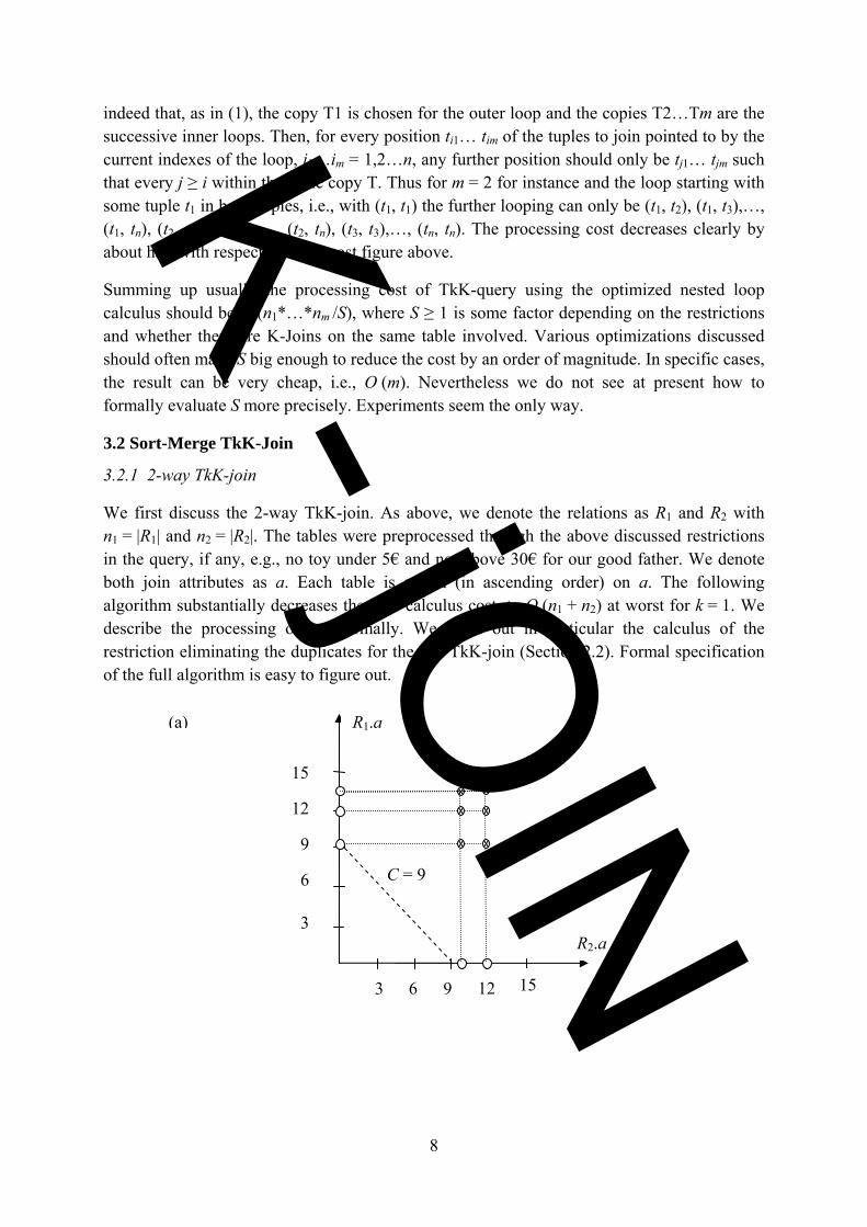
We first discuss the 2-way TkK-join. As above, we denote the relations as R1 and R2 with n1 = |R1| and n2 = |R2|. The tables were preprocessed through the above discussed restrictions in the query, if any, e.g., no toy under 5€ and not above 30€ for our good father. We denote both join attributes as a. Each table is sorted (in ascending order) on a. The following algorithm substantially decreases then the calculus cost, to O (n1 + n2) at worst for k = 1. We describe the processing only informally. We leave out in particular the calculus of the restriction eliminating the duplicates for the self TkK-join (Section 2.2). Formal specification of the full algorithm is easy to figure out.
3
6
9
12
15
3 6 9 12 15
C = 9
R1.a
R2.a
(a) K - jO
IN
9
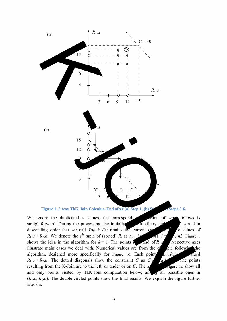
Figure 1. 2-way TkK-Join Calculus. End after (a) Step 1, (b) Step 2, (c) Steps 3-6.
We ignore the duplicated a values, the corresponding extension of what follows is straightforward. During the processing, the initially empty auxiliary table T[1..k] sorted in descending order that we call Top k list retains the current candidate Top k values of R1.a + R2.a. We denote the ith tuple of (sorted) Rj as ti,j ; i = 1,2…n1, j = 1,2…n2. Figure 1 shows the idea in the algorithm for k = 1. The points R1.a and of R2.a at respective axes illustrate main cases we deal with. Numerical values are from the example following the algorithm, designed more specifically for Figure 1c. Each point (R1.a, R2.a) is valued R1.a + R2.a. The dotted diagonals show the constraint C as C = R1.a + R2.a. The points resulting from the K-Join are to the left, or under or on C. The arrows of Figure 1c show all and only points visited by TkK-Join computation below, among all possible ones in (R1.a, R2.a). The double-circled points show the final results. We explain the figure further later on.
3
6
9
12
15
3 6 9 12 15
C =15
R1.a
R2.a
(c)
3
6
9
12
15
3 6 9 12 15
C = 30
R1.a
R2.a
(b) K - jOIN
10
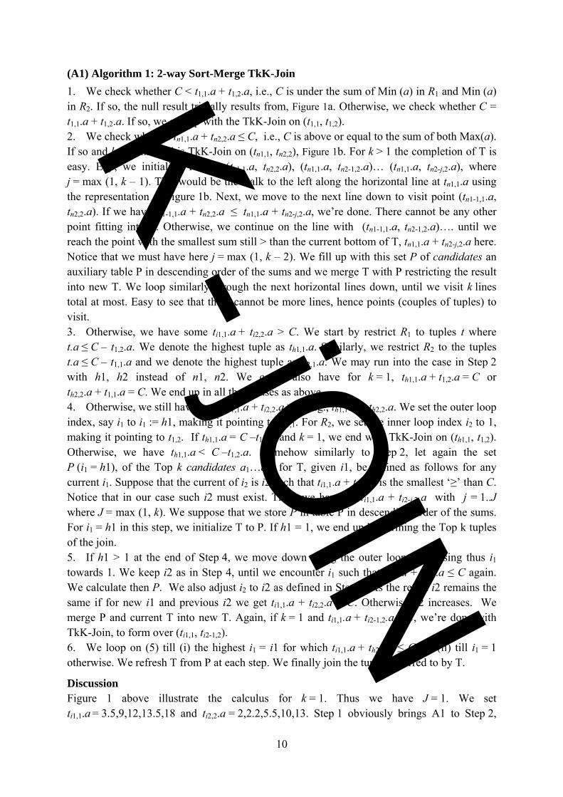
(A1) Algorithm 1: 2-way Sort-Merge TkK-Join 1. We check whether C < t1,1.a + t1,2.a, i.e., C is under the sum of Min (a) in R1 and Min (a) in R2. If so, the null result trivially results from, Figure 1a. Otherwise, we check whether C = t1,1.a + t1,2.a. If so, we end up with the TkK-Join on (t1,1, t1,2). 2. We check whether tn1,1.a + tn2,2.a ≤ C, i.e., C is above or equal to the sum of both Max(a). If so and k = 1, the end is TkK-Join on (tn1,1, tn2,2), Figure 1b. For k > 1 the completion of T is easy. E.g., we initialize T with (tn1,1.a, tn2,2.a), (tn1,1.a, tn2-1,2.a)… (tn1,1.a, tn2-j,2.a), where j = max (1, k – 1). This would be the walk to the left along the horizontal line at tn1,1.a using the representation at Figure 1b. Next, we move to the next line down to visit point (tn1-1,1.a, tn2,2.a). If we have tn1-1,1.a + tn2,2.a ≤ tn1,1.a + tn2-j,2.a, we’re done. There cannot be any other point fitting into T. Otherwise, we continue on the line with (tn1-1,1.a, tn2-1,2.a)…. until we reach the point with the smallest sum still > than the current bottom of T, tn1,1.a + tn2-j,2.a here. Notice that we must have here j = max (1, k – 2). We fill up with this set P of candidates an auxiliary table P in descending order of the sums and we merge T with P restricting the result into new T. We loop similarly through the next horizontal lines down, until we visit k lines total at most. Easy to see that there cannot be more lines, hence points (couples of tuples) to visit. 3. Otherwise, we have some ti1,1.a + ti2,2.a > C. We start by restrict R1 to tuples t where t.a ≤ C – t1,2.a. We denote the highest tuple as th1,1.a. Similarly, we restrict R2 to the tuples t.a ≤ C – t1,1.a and we denote the highest tuple as th2,1.a. We may run into the case in Step 2 with h1, h2 instead of n1, n2. We could also have for k = 1, th1,1.a + t1,2.a = C or th2,2.a + t1,1.a = C. We end up in all these cases as above. 4. Otherwise, we still have some ti1,1.a + ti2,2.a > C, e.g., th1,1.a + th2,2.a. We set the outer loop index, say i1 to i1 := h1, making it pointing to th1,1. For R2, we set the inner loop index i2 to 1, making it pointing to t1,2. If th1,1.a = C –t1,2.a and k = 1, we end with TkK-Join on (th1,1, t1,2). Otherwise, we have th1,1.a < C –t1,2.a. Somehow similarly to Step 2, let again the set P (i1 = h1), of the Top k candidates a1…aJ for T, given i1, be defined as follows for any current i1. Suppose that the current of i2 is i2 such that ti1,1.a + ti2,2.a is the smallest ‘≥’ than C. Notice that in our case such i2 must exist. Then, we have aj = ti1,1.a + ti2-j,2.a with j = 1..J where J = max (1, k). We suppose that we store P in table P in descending order of the sums. For i1 = h1 in this step, we initialize T to P. If h1 = 1, we end up by forming the Top k tuples of the join. 5. If h1 > 1 at the end of Step 4, we move down along the outer loop, decreasing thus i1 towards 1. We keep i2 as in Step 4, until we encounter i1 such that ti1,1.a + ti2,2.a ≤ C again. We calculate then P. We also adjust i2 to i2 as defined in Step 4. As the result i2 remains the same if for new i1 and previous i2 we get ti1,1.a + ti2,2.a = C. Otherwise, i2 increases. We merge P and current T into new T. Again, if k = 1 and ti1,1.a + ti2-1,2.a = C, we’re done with TkK-Join, to form over (ti1,1, ti2-1,2). 6. We loop on (5) till (i) the highest i1 = i1 for which ti1,1.a + th2,2.a ≤ C or (ii) till i1 = 1 otherwise. We refresh T from P at each step. We finally join the tuples referred to by T.
Discussion Figure 1 above illustrate the calculus for k = 1. Thus we have J = 1. We set ti1,1.a = 3.5,9,12,13.5,18 and ti2,2.a = 2,2.2,5.5,10,13. Step 1 obviously brings A1 to Step 2,
K - jOIN
11
since 3.5+2 < 15. We pass Step 2 since 18+13 > 15. Step 3 at first bypasses t5,1.a = 18 and t4,1.a = 13.5, since 15 > 13.5 + 2. We arrive to t3,1.a = 12 and to t4,2.a = 10, , hence to h1 = 3 and h2 = 10. None of the conditions which would make A1 stopping in this step verifies. We thus pass to Step 4.
Here, we start with t4,1.a = 12 and t1,2.a = 2. The sum is below 15, hence A1 continues. We adjust i2 to 3, since the point t4,1.a + t2,3.a = 12 + 5.5 is the smallest ≥ 15 for our h1, i.e., on the corresponding horizontal line at the figure. There only one candidate for P is (t4,1.a, t2,2.a) = (12, 2.2), labeled with 14.2. We initialize T accordingly. Since h1 > 1, we move to Step 5.
Here, we move down along the vertical line starting at (12, 5.5) at the figure. We arrive to (9, 5.5) labeled with 14.5. We have i1 = 2 and we adjust i2 to i2 = 3. New P has the element (9, 5.5). Since it is above the current value 14.2 in T, we update T accordingly. T points now to the new tuple.
Since 14.5 ≠ 15, A1 starts Step 6. Here we loop according to vertical and horizontal lines at the figure. This until we reach t1,1.a = 3.5. The horizontal move there ends at t5,2.a = 13. The last P contains thus the candidate (3.5, 10). This one does not make thus to T. One can easily check that the same holds for every other candidate after (9, 5.5). A1 joins therefore the two related tuples. This is the correct result for the related TkK-Join.
Notice from the figure that A1 avoids joining most of the tuples that the generic K-Join calculus for TkK-Join would do. For instance, if R1 and R2 had only 16K tuples remaining after the restrictions, A1 would avoid up to 256M – 32k tuples for k = 1, i.e., more than 99.99 %! That is why it should be usually much faster. Here, it would be up to 8000 times. This represents, e.g., 12s instead of more than 24h. Observe also that if TkK-Join concerns the self TkK-join of a table T sorted over the join attribute, with, say, n tuples, the worst complexity can be only O (n) for k = 1. We skipped this detail from A1 specs, but we only need to match over the tuples (ti1, ti2) with i1 = n,n-1…; i2 = 1,2… and i1 ≥ i2.
It is not difficult, although tedious, to see that A1 is correct, i.e., that there cannot be any missed choice for the Top k list. The worst case speed of O (n1 + n2) we have announced for k = 1 is easily seen from the figure. For k >1 it should be O (n1 + kn2), given the maximal size of P at each step of the outer loop. The latter evaluation seems nevertheless by far too pessimistic in practice, somehow like the similar one for the hashing. We leave a more accurate study for the future. The usual speed for k = 1should be somehow moderately faster than the worst one as well. Especially, in the absence of any additional selectivity knowledge, we can consider that even only the restriction in Step 2, on the average reduces the size of the table by half. So it cuts down the processing cost.
3.2.2 Sort-Merge m-way K-Join
We now generalize the algorithm to m-way K-Join with m > 2. We thus have m tables R1…Rm to join, all being ordered. In fact, as it will appear, while the ordering of two tables, say of R1 and of R2 is crucial for the speed, the ordering of the remaining tables only may make faster the processing of the restriction selecting a fraction of a table. Consider indeed as usual that
K - jOIN
12
every c value in the table is equally likely and that the search is sequential, upward or downward, depending on which seems faster. If f is a fraction of a table with n tuples, the average cost is then the smaller of O (fn) or of O ((1-f)n). The cost for unordered table is O (n), we recall.
The restrictions from Step 3 generalize obviously. Namely, the one for any table Rj ; j =1,...m is that we only keep any tuple tj such that tj.c ≤ C – t1,i1.c… t1,im-1.c where i1…im-1 are all different of ij. The rest of the algorithm remains the same, applying to tables R1 and R2 among m. However A1 is now re-executed for any possible combination of the tuples tim,m… ti3,3. The rationale is that any such combination has the potential of making the best for Top k K-Join the combination tim,m… ti3,3 ti2,2 ti1,1 with any any two tuples ti2,2, ti1,1 that were not the among the Top k for the previously visited combination tin,n… ti3,3.
Figure 1 is instructive also for 3-way join. Consider indeed that we visit R3 tuples in ascending order on join attribute t3.c. The dashed line for C = 15 could correspond to the minimal value of t3.c, after the above restrictions. After the calculus at the figure, next value of t3.c would lead to a new line, necessarily to the left of the one at the figure. And so on. Each new calculus should be faster than the previous one. We do not see however how to estimate this acceleration formally at present.
The algorithm is notably faster than the nested loop one, because of its sort-merge 2-way part. The processing cost (speed) is O (nm*…n3(n2 + n1)). For instance thus if the initial tables R1 and R2 had 16K tuples each, after the restrictions, the speed-up would be (again) 8K times, regardless of the size of the other tables. The cost of the restrictions depends on their selectivity, as above mentioned.
If the tables involved in the TkK-Join have quite different sizes, after the restrictions, then one should choose for R1 and R2 the longest ones. These are the most advantageous for (n2+n1) component in the above speed complexity formula. Otherwise there form some ni*ni+1 contribution. To appreciate the savings, consider that we evaluate for the 3-way join the choice n1 = 1K n2 = n3 =1M versus the alternative one n2 = n3 =1M n3 = 1K. The former choice provides the speed of O (1K*(1M+1M) ≅ O (2G). The latter one leads similarly to the speed of about O (1T). This one is 500 times longer, e.g., 8m versus 1s.
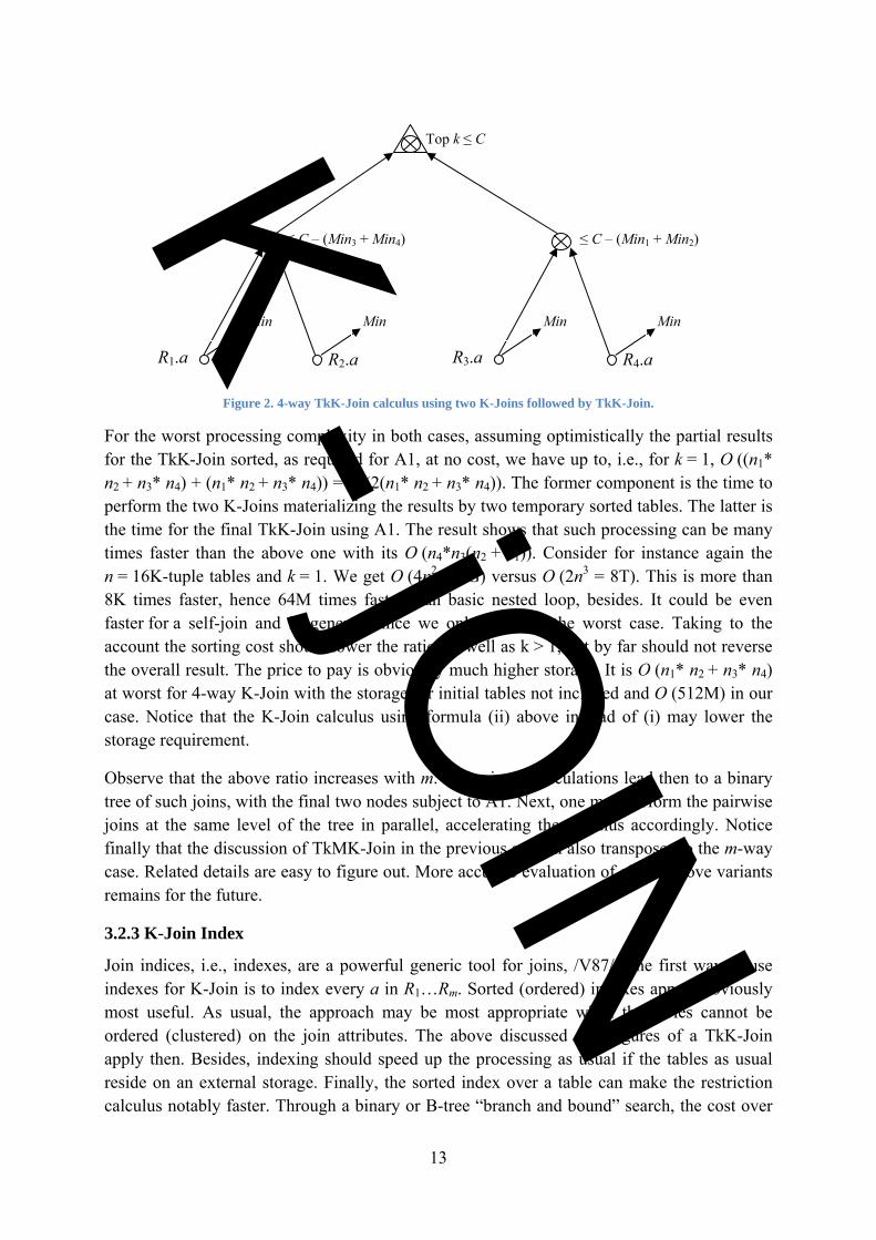
The above way to calculate an m-way join is nevertheless neither the only possible nor even always potentially the fastest. For instance, using formula (5), one may calculate a 4-way TkK-Join also over the results of 2 pairwise K-Joins, over R1 and R2 and R3 and R4 respectively. These can be, e.g. for R1 and R2, (i) R1.a + R2.a ≤ C or (ii) R1.a + R2.a ≤ C –(Min(R3.c) + Min(R4.c)), Figure 2. The latter formulae may decrease the storage requirements that we show below for the worst case, as well as the total time, especially if the DBMS maintains the Min statistics as usual.
K - jOIN
13
Figure 2. 4-way TkK-Join calculus using two K-Joins followed by TkK-Join.
For the worst processing complexity in both cases, assuming optimistically the partial results for the TkK-Join sorted, as required for A1, at no cost, we have up to, i.e., for k = 1, O ((n1* n2 + n3* n4) + (n1* n2 + n3* n4)) = O (2(n1* n2 + n3* n4)). The former component is the time to perform the two K-Joins materializing the results by two temporary sorted tables. The latter is the time for the final TkK-Join using A1. The result shows that such processing can be many times faster than the above one with its O (n4*n3(n2 + n1)). Consider for instance again the n = 16K-tuple tables and k = 1. We get O (4n2 = 1G) versus O (2n3 = 8T). This is more than 8K times faster, hence 64M times faster than basic nested loop, besides. It could be even faster for a self-join and in general, since we only consider the worst case. Taking to the account the sorting cost should lower the ratio, as well as k > 1, but by far should not reverse the overall result. The price to pay is obviously much higher storage. It is O (n1* n2 + n3* n4) at worst for 4-way K-Join with the storage for initial tables not included and O (512M) in our case. Notice that the K-Join calculus using formula (ii) above instead of (i) may lower the storage requirement.
Observe that the above ratio increases with m. Pairwise K-calculations lead then to a binary tree of such joins, with the final two nodes subject to A1. Next, one may perform the pairwise joins at the same level of the tree in parallel, accelerating the calculus accordingly. Notice finally that the discussion of TkMK-Join in the previous section also transposes to the m-way case. Related details are easy to figure out. More accurate evaluation of all the above variants remains for the future.
3.2.3 K-Join Index
Join indices, i.e., indexes, are a powerful generic tool for joins, /V87/. The first way to use indexes for K-Join is to index every a in R1…Rm. Sorted (ordered) indexes appear obviously most useful. As usual, the approach may be most appropriate when the tables cannot be ordered (clustered) on the join attributes. The above discussed cost figures of a TkK-Join apply then. Besides, indexing should speed up the processing as usual if the tables as usual reside on an external storage. Finally, the sorted index over a table can make the restriction calculus notably faster. Through a binary or B-tree “branch and bound” search, the cost over
R2.a R1.a
Min Min
R4.a R3.a
Min Min
≤ C – (Min3 + Min4) ≤ C – (Min1 + Min2)
Top k ≤ C K - jOIN
14
n-tuple table may decrease to O (log n) at most, instead of O (n) basically, we recall. In particular, A1 and its m-way extension apply almost as is to such indices.
Next possibility for K-Join indexing is a sorted index, say IK, over m-way C values. Assuming that this index is a relational table, we create for each K-join tuple t1…tm, at least the entry (C, t1.Id,…, tm.Id) with C = t1.a+…+tm.a. At least, since indexing also some or every ti.a may speed up queries with conditions on those, in the absence or even presence of the single table indexes. Such as “every price should differ from C /m by 10% at most”. An IK may be thought about also as a materialized K-join view, i.e. by straight analogy to materialized join views. Notice that the SQL Server terminology for a materialized view is rather an indexed view. The indexed views in SQL Server 2005, besides, basically did not support self-join. Thus, whether one can create self K-join views there remains subject to experimentation at present. Since only TkK queries are of interest here, we see IK sorted on C first, then on some or all other key or non-key attributes. An IK has the storage cost of O (n1*…*nm) in general. It is about half of it for copies of the same table. The figure may be obviously consequent. But is not prohibitive in practice for tables of a couple of thousands of tuples and for m = 2…4 and perhaps up to m = 8 occasionally.
For 1K-tuple tables indeed, 3-way K-Join index would be 1G-entry, so would likely use O (6G) bytes in practice. Such index could even be RAM resident and certainly enters a current flash disk. The 4-way index would have 1T entries, in line with the capacity of one or a few of current popular disk devices. In our toy example, the 2-way index would have little less than 128M entries (under half of 16K2) and 3-way index would contain almost 2G entries. Again, OK for most current computer. However, the 4-way index size would already be prohibitive for a popular use, with about 32T entries. It qualifies nevertheless potentially for a cloud implementation as we discuss later on. On the other hand, consider that we have after the restrictions, several, smaller but still practical 1K tuple tables to TkK-Join. Then 4-way IK would have “only” 1G entries and 5-way one would have 1T entries. Both are easily stored at popular hardware, the former even in RAM.
While the storage cost of a join index is a drawback, the TkK-Join processing becomes orders of magnitude faster. Indeed, it is in the order of O (log |IK|) visited entries. Thus for a 1T-entry and the 5-way TkK-Join, we are at about O (30) entries. It is instructive to compare to the basic cost of 1K5= 1P entries visited, characteristic of any current DBMS, we recall. As well as to our best cost without a join index that would be in the orders of O (2T) entries visited. In practice, one would rather use a B+-tree of some kind for a T-entry index. Our figure would boil to a few disk accesses, hence to the timing of a fraction of a second.
One may finally observe that m-way TkK-join indexes speed up also the calculus of m’-way TkK-joins, m’ > m. For m’ = 2m, the time is in particular O (|I1
K|+|I2K|) through A1 over C-
values in both m-way indices. Thus, in our example of 1K-tuple tables, a 6-way TkK-join over two 3-way indexes would require about 2G entries visited for 6 different tables and little less than 1G entries for (the virtual copies of) a single table. At each choice of entries visited there is an addition and a test performed. At the current speed of the hardware, a popular 4-core appears to easily handle about 250M additions with the test per second. The 6-way TkK-
K - jOIN
15
join would require a few seconds. However, the 8-way TkK-join using thus two 1T-entry indices for 1K tables would remain clearly typically impractical, lasting for hours.
Again, it is instructive to compare the above 6-way timing to the basic one and the other methods above. The generic calculus, characteristic of any prominent DBMS as by today, we recall, would require O (1E) operations (steps in the loop). It means an eternity in practice. Even the sort-merge TkK-join would require O (2P) operations. Hence, our join indices accelerate the calculus 1M times. In these conditions, it becomes even worth to dynamically create the indexes. Their cost is indeed in our example close to O (4-5G), depending on the specifics of the dynamic creation of a sorted file. Hence, the speed-up remains about 100K times. Finally, we recall that if the m-way TkK-join operates over a single table, with its virtual copies, the space cost of the index should divide by about two usually, increasing the speed-up accordingly.
The downside of a TkK-join index is its, already discussed, creation cost, but also the maintaince cost. Adding a tuple to table Rj involved in m-way join index costs O (n1*…*nj-1* nj+1*…*nm) new tuples to create. Similar costs characterize a tuple update or deletion. To ease these operations it may be useful to store also all the (m-1)-way indexes. Their storage cost should be usually negligible compared to that of the m-way one. Application dependent constraints have to determine best compromises. Sometimes it may be more useful for instance to have two m/2 – way indexes than a single m-way one.
3.2.4 Cloud TkK-Join Processing
One approach is as follows. Consider we have (a cloud, P2P net, grid… of) M nodes. We replicate each table R1…Rm-1 on every node. We partition, e.g., by hash, table Rm into M segments, one per node. At each node, we perform the join as above discussed. We collect the results at some node where the final selection of k tuples takes place.
The processing cost is obviously close to 1/M of the centralized one, whether one performs the nested or sort-merge TkK-Join.
Another possibility is the distributed and parallel evaluation of the pairwise joins hinted to in Section 3.2.2 above. This includes the processing of the intermediate results in the tree that one can also evaluate in parallel. The formulae in Section 3.2.2 imply that the result may be faster than the above. The cloud can easily provide for TBs of storage possibly needed for the intermediate results when tables or m are larger and perhaps lacking on a stand-alone system. In fact, the cloud appears the only practical approach for many K-tuple tables and a larger m like m = 8. Deeper evaluation of this approach remains a future goal.
Yet another and potentially even faster way is to distribute the join indexes. A TkK-join index being a sorted 1-d index, many schemes exist for such a distribution. For instance, one can choose our RP*S scheme, /LNS94/, especially for a larger number of nodes, e.g. M = 1K. This opens the perspective of managing very large indexes with fast calculus of very large joins. For instance the 4-way 1T entry index we had discussed, for our 1K-tuple tables, would end up in the 1K-node cloud with 1G entry per node. This qualifies for basic flash storage. The TkK-join calculus for which the index has been created should typically visit only one node.
K - jOIN
16
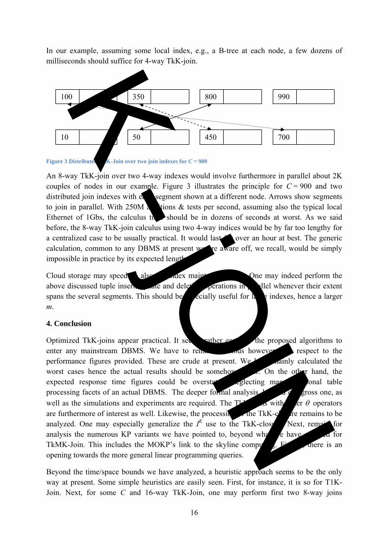
In our example, assuming some local index, e.g., a B-tree at each node, a few dozens of milliseconds should suffice for 4-way TkK-join.
Figure 3 Distributed TkK-Join over two join indexes for C = 900
An 8-way TkK-join over two 4-way indexes would involve furthermore in parallel about 2K couples of nodes in our example. Figure 3 illustrates the principle for C = 900 and two distributed join indexes with each segment shown at a different node. Arrows show segments to join in parallel. With 250M additions & tests per second, assuming also the typical local Ethernet of 1Gbs, the calculus time should be in dozens of seconds at worst. As we said before, the 8-way TkK-join calculus using two 4-way indices would be by far too lengthy for a centralized case to be usually practical. It would last for over an hour at best. The generic calculation, common to any DBMS at present we are aware off, we recall, would be simply impossible in practice by its expected length.
Cloud storage may speed up also the index maintenance time. One may indeed perform the above discussed tuple insert, update and deletion operations in parallel whenever their extent spans the several segments. This should be especially useful for large indexes, hence a larger m.
4. Conclusion
Optimized TkK-joins appear practical. It seems rather easy for the proposed algorithms to enter any mainstream DBMS. We have to remain cautious however with respect to the performance figures provided. These are crude at present. We have mainly calculated the worst cases hence the actual results should be somehow better. On the other hand, the expected response time figures could be overstated, neglecting many relational table processing facets of an actual DBMS. The deeper formal analysis, beyond our gross one, as well as the simulations and experiments are required. The TkK-Joins with other θ operators are furthermore of interest as well. Likewise, the processing of the TkK-closure remains to be analyzed. One may especially generalize the IK use to the TkK-closure. Next, remain for analysis the numerous KP variants we have pointed to, beyond what we have outlined for TkMK-Join. This includes the MOKP’s link to the skyline computing. Finally, there is an opening towards the more general linear programming queries.
Beyond the time/space bounds we have analyzed, a heuristic approach seems to be the only way at present. Some simple heuristics are easily seen. First, for instance, it is so for T1K-Join. Next, for some C and 16-way TkK-Join, one may perform first two 8-way joins
100 350 800 990
10 50 450 700
K - jOIN
17
selecting each TOP k tuples which are the closest to C/2, e.g., k/2 under and k/2 above. Then, one may reduce both lists by performing the TkK-Join with respect k tuples and C over them. The rule obviously generalizes to m > 16. The heuristic processing of larger TkK-Joins is also the future investigation. This should be based on the numerous results of the operations research. The scalable distributed one in a cloud with its scan, i.e., Map/Reduce, capability appears especially interesting for both the exact and the approximate result.
Acknowledgments. Lionel Delafosse helped with experiments on the speed of additions accompanied by the “≤ C” test and the write to a memory for some, over a popular 4-core Wintel PC. Tore Risch observed the future opening towards the linear programming. Finally, we are especially grateful to Federico Della Croce (Politecnico di Torino) for the update on the state-of-the-art of KP research in the combinatorial optimization “chapel”.
References
/BHV9/ Bazgan, C., Hugot, H., Vanderpooten, D. Solving efficiently the 0-1 multi-objective knapsack problem. C& OR. 36, 1, Jan. 2009, 260-279. /LNS94/ Litwin, W., Neimat, M-A., Schneider, D. RP* : A Family of Order Preserving Scalable Distributed Data Structures (VLDB-94). /MT90/ Martello, S., Toth, P. Knapsack Problems. John Wiley and Sons, 1990. /OR-L/ Or-Library. http://people.brunel.ac.uk/~mastjjb/jeb/info.html /PRP9/ Puchinger, J., Raidl, G. R., Pferschy, U. The Multidimensional Knapsack Problem: Structure and Algorithms. INFORMS JOURNAL ON COMPUTING, 2009. /QST09/ Quadri, D., Soutif, E., Tolla, P. Exact solution method to solve large scale integer quadratic multidimensional knapsack problems. Journal of Combinatorial Optimization. 17, 2, 2009, 157-167. /V87/ P. Valduriez. Join Indices. ACM Trans. Database Systems, vol. 12, no. 2, 1987. /VKB10/ Venkatesan, D., Kannan, K., Balachandar, S. R. Centre Of Mass Selection Operator Based Meta-Heuristic For Unbounded Knapsack Problem. Intl. J. of Math. and Stat. Sciences 2:1 2010 /W9/ List of knapsack problems. Wikipedia. http://en.wikipedia.org/wiki/List_of_knapsack_problems
K - jO
IN


![[k] summer 2010](https://static.fdocument.org/doc/165x107/568bf3b91a28ab89339b61c6/k-summer-2010.jpg)