Time Dependent Perturbation Theory - MIT OpenCourseWare · 74 CHAPTER 4. TIME DEPENDENT...

Chapter 4

Time Dependent PerturbationTheory

c© B. Zwiebach

4.1 Time dependent perturbations

We will assume that, as before, we have a Hamiltonian H(0) that is known and is timeindependent. Known means we know the spectrum of energy eigenstates and the energyeigenvalues. This time the perturbation to the Hamiltonian, denoted as δH(t) will be timedependent and, as a result, the full Hamiltonian H(t) is also time dependent

H(t) = H(0) + δH(t) . (4.1.1)

While H(0) has a well-defined spectrum, H(t) does not. Being time dependent, H(t) doesnot have energy eigenstates. It is important to remember that the existence of energyeigenstates was predicated on the factorization of solutions Ψ(x, t) of the full Schrodingerequation into a space-dependent part ψ(x) and a time dependent part that turned out to bee−iEt/~, with E the energy. Such factorization is not possible when the Hamiltonian is timedependent. Since H(t) does not have energy eigenstates the goal is to find the solutions|Ψ(x, t)〉 directly. Since we are going to focus on the time dependence, we will suppress thelabels associated with space. We simply say we are trying to find the solution |Ψ(t)〉 to theSchrodinger equation

i~∂

∂t|Ψ(t)〉 =

(H(0) + δH(t)

)|Ψ(t)〉 . (4.1.2)

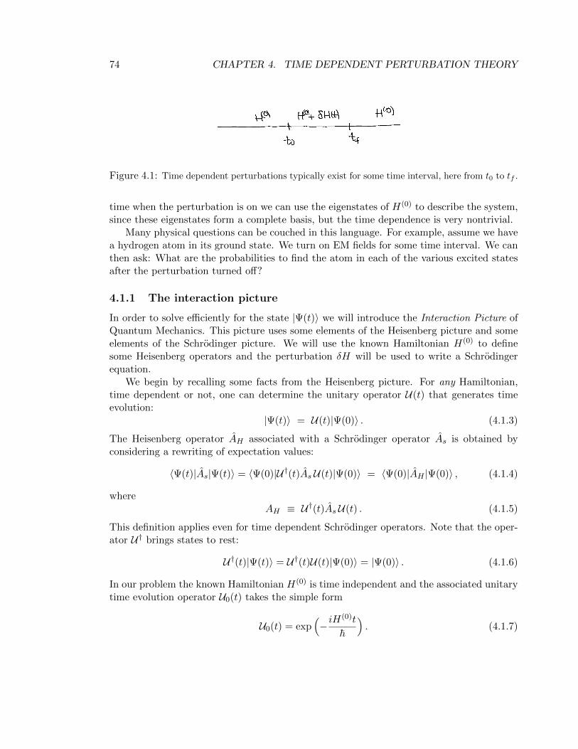
In typical situations the perturbation δH(t) vanishes for t < t0, it exists for some finitetime, and then vanishes for t > tf (see Figure 4.1). The system starts in an eigenstate ofH(0) at t < t0 or a linear combination thereof. We usually ask: What is the state of thesystem for t > tf? Note that both initial and final states are nicely described in terms ofeigenstates of H(0) since this is the Hamiltonian for t < t0 and t > tf . Even during the

73

74 CHAPTER 4. TIME DEPENDENT PERTURBATION THEORY

Figure 4.1: Time dependent perturbations typically exist for some time interval, here from t0 to tf .

time when the perturbation is on we can use the eigenstates of H(0) to describe the system,since these eigenstates form a complete basis, but the time dependence is very nontrivial.

Many physical questions can be couched in this language. For example, assume we havea hydrogen atom in its ground state. We turn on EM fields for some time interval. We canthen ask: What are the probabilities to find the atom in each of the various excited statesafter the perturbation turned off?

4.1.1 The interaction picture

In order to solve efficiently for the state |Ψ(t)〉 we will introduce the Interaction Picture ofQuantum Mechanics. This picture uses some elements of the Heisenberg picture and someelements of the Schrodinger picture. We will use the known Hamiltonian H(0) to definesome Heisenberg operators and the perturbation δH will be used to write a Schrodingerequation.

We begin by recalling some facts from the Heisenberg picture. For any Hamiltonian,time dependent or not, one can determine the unitary operator U(t) that generates timeevolution:

|Ψ(t)〉 = U(t)|Ψ(0)〉 . (4.1.3)

The Heisenberg operator AH associated with a Schrodinger operator As is obtained byconsidering a rewriting of expectation values:

〈Ψ(t)|As|Ψ(t)〉 = 〈Ψ(0)|U†(t)As U(t)|Ψ(0)〉 = 〈Ψ(0)|AH |Ψ(0)〉 , (4.1.4)

whereAH ≡ U†(t)As U(t) . (4.1.5)

This definition applies even for time dependent Schrodinger operators. Note that the oper-ator U† brings states to rest:

U†(t)|Ψ(t)〉 = U†(t)U(t)|Ψ(0)〉 = |Ψ(0)〉 . (4.1.6)

In our problem the known Hamiltonian H(0) is time independent and the associated unitarytime evolution operator U0(t) takes the simple form

U0(t) = exp(− iH

(0)t

~

). (4.1.7)

4.1. TIME DEPENDENT PERTURBATIONS 75

The state |Ψ(t)〉 in our problem evolves through the effects of H(0) plus δH. Motivatedby (4.1.6) we define the auxiliary ket

∣∣Ψ(t)⟩

as the ket |Ψ(t)〉 partially brought to rest

through H(0): ∣∣Ψ(t)⟩≡ exp

( iH(0)t

~

)∣∣Ψ(t)⟩. (4.1.8)

Expect that Schrodinger equation for∣∣Ψ(t)

⟩will be simpler, as the above must have taken

care of the time dependence generated by H(0). Of cours, if we can determine∣∣Ψ(t)

⟩we

can easily get back the desired state∣∣Ψ(t)

⟩inverting the above relation to find

∣∣Ψ(t)⟩

= exp(− iH

(0)t

~

)∣∣Ψ(t)⟩. (4.1.9)

Our objective now is to find the Schrodinger equation for∣∣Ψ(t)

⟩. Taking the time

derivative of (4.1.8) and using (4.1.2)

i~d

dt

∣∣Ψ(t)⟩

= −H(0)∣∣Ψ(t)

⟩+ exp

( iH(0)t

~

)(H(0) + δH(t))

∣∣Ψ(t)⟩

=

[−H(0) + exp

( iH(0)t

~

)(H(0) + δH(t)) exp

(− iH

(0)t

~

)]∣∣Ψ(t)⟩

= exp( iH(0)t

~

)δH(t) exp

(− iH

(0)t

~

)∣∣Ψ(t)⟩, (4.1.10)

where the dependence on H(0) cancelled out. We have thus found the Schrodinger equation

i~d

dt

∣∣Ψ(t)⟩

= δH(t)∣∣Ψ(t)

⟩. (4.1.11)

where the operator δH(t) is defined as

δH(t) ≡ exp( iH(0)t

~

)δH(t) exp

(− iH

(0)t

~

). (4.1.12)

Note that as expected the time evolution left in∣∣Ψ(t)

⟩is generated by δH(t) via a Schrodinger

equation. The operator δH(t) is nothing else but the Heisenberg version of δH generatedusing H(0)! This is an interaction picture, a mixture of Heisenberg’s and Schrodinger pic-ture. While we have some Heisenberg(0) operators there is still a time dependent state∣∣Ψ(t)

⟩and a Schrodinger equation for it.


How does it all look in an orthonormal basis? Let |n〉 be the complete orthonormal basisof states for H(0):

H(0)|n〉 = En|n〉 . (4.1.13)

This time there is no need for a (0) superscript, since neither the states nor their energieswill be corrected (there are no energy eigenstates in the time-dependent theory). We thenwrite an ansatz for our unknown ket:∣∣Ψ(t)

⟩=∑n

cn(t)|n〉 . (4.1.14)

Here the functions cn(t) are unknown. This expansion is justified since the states |n〉 forma basis, and thus at all times they can be used to describe the state of the system. Theoriginal wavefunction is then:

∣∣Ψ(t)⟩

= exp(− iH

(0)t

~

)∣∣Ψ(t)⟩

=∑n

cn(t) exp

(− iEnt

~

)|n〉 . (4.1.15)

Note that the time dependence due to H(0) is present here. If we had δH = 0 the state∣∣Ψ(t)⟩

would be a constant, as demanded by the Schrodinger equation (4.1.11) and thecn(t) would be constants. The solution above would give the expected time evolution of thestates under H(0).

To see what the Schrodinger equation tells us about the functions cn(t) we plug theansatz (4.1.14) into (4.1.11):

i~d

dt

∑m

cm(t)|m〉 = δH(t)∑n

cn(t)|n〉 (4.1.16)

Using dots for time derivatives and introducing a resolution of the identity on the right-handside we find ∑

m

i~cm(t)|m〉 =∑m

|m〉〈m|δH(t)∑n

cn(t)|n〉

=∑m

|m〉∑n

〈m|δH(t)|n〉cn(t)

=∑m,n

δHmn(t)cn(t)|m〉 . (4.1.17)

Here we have used the familiar matrix element notation

δHmn(t) ≡ 〈m|δH(t)|n〉 . (4.1.18)

Equating the coefficients of the basis kets |m〉 in (4.1.17) we get the equations

i~ cm(t) =∑n

δHmn(t) cn(t) . (4.1.19)


The Schrodinger equation has become an infinite set of coupled first-order differential equa-tions. The matrix elements in the equation can be simplified a bit by passing to un-tildevariables:

δHmn(t) =⟨m∣∣ exp

( iH(0)t

~

)δH(t) exp

(− iH

(0)t

~

)∣∣n⟩= exp

[i

~(Em − En)t

]〈m|δH(t)|n〉 .

(4.1.20)

If we define

ωmn ≡Em − En

~, (4.1.21)

we then haveδHmn(t) = eiωmntδHmn(t) . (4.1.22)

The coupled equations (4.1.19) for the functions cn(t) then become

i~ cm(t) =∑n

eiωmntδHmn(t)cn(t) . (4.1.23)

4.1.2 Example (based on Griffiths Problem 9.3)

Consider a two-state system with basis states |a〉 and |b〉, eigenstates of H(0) with energiesEa and Eb, respectively. Call

ωab ≡ (Ea − Eb)/~ . (4.1.24)

Now take the perturbation to be a matrix times a delta function at time equal zero. Thusthe perturbation only exists for time equal zero:

δH(t) =

(0 αα∗ 0

)δ(t) ≡ U δ(t) , (4.1.25)

where α is a complex number. With the basis vectors ordered as |1〉 = |a〉 and |2〉 = |b〉 wehave

U =

(Uaa UabUba Ubb

), with Uaa = Ubb = 0 and Uab = U∗ba = α . (4.1.26)

There is a sudden violent perturbation at t = 0 with off-diagonal elements that shouldproduce transition. Take the system to be in |a〉 for t = −∞, what is the probability thatit is in |b〉 for t = +∞?

Solution: First note that if the system is in |a〉 at t = −∞ it will remain in state |a〉 untilt = 0−, that is, just before the perturbation turns on. This is because |a〉 is an energyeigenstate of H(0). In fact we have, up to a constant phase,

|Ψ(t)〉 = e−iEat/~|a〉 , for −∞ < t ≤ 0− . (4.1.27)


We are asked what will be the probability to find the state in |b〉 at t =∞, but in fact, theanswer is the same as the probability to find the state in |b〉 at t = 0+. This is because theperturbation does not exist anymore and if the state at t = 0+ is

|Ψ(0+)〉 = γa|a〉+ γb |b〉 , (4.1.28)

with γ1 and γ2 constants, then the state for any time t > 0 will be

|Ψ(t)〉 = γa|a〉e−iEat/~ + γb|b〉e−iEbt/~ . (4.1.29)

The probability pb(t) to find the state |b〉 at time t will be

pb(t) = |〈b|Ψ(t)〉|2 =∣∣∣γbe−iEbt/~∣∣∣ = |γb|2 , (4.1.30)

and, as expected, this is time independent. It follows that to solve this problem we mustjust find the state at t = 0+ and determine the constants γ1 and γ2.

Since we have two basis states the unknown tilde state is∣∣Ψ(t)⟩

= ca(t)|a〉+ cb(t)|b〉 , (4.1.31)

and the initial conditions are stating that the system begins in the state |a〉 are

ca(0−) = 1 , cb(0

−) = 0 . (4.1.32)

The differential equations (4.1.23) take the form

i~ ca(t) = eiωabtδHab(t)cb(t) ,

i~ cb(t) = eiωbatδHba(t)ca(t) .(4.1.33)

The couplings are off-diagonal because δHaa = δHbb = 0. Using the form of the δH matrixelements,

i~ ca(t) = eiωabt α δ(t) cb(t) ,

i~ cb(t) = e−iωabt α∗δ(t) ca(t) .(4.1.34)

We know that for functions f continuous at t = 0 we have f(t)δ(t) = f(0)δ(t). We nowask if we are allowed to use such identity for the right-hand side of the above equations. Infact we can use the identity for e±iωabt but not for the functions ca(t) and cb(t) that, areexpected to be discontinuous at t = 0. They must be so, because they can only change att = 0, when the delta function exists. Evaluating the exponentials at t = 0 we then get thesimpler equations

i~ ca(t) = α δ(t) cb(t) ,

i~ cb(t) = α∗δ(t) ca(t) .(4.1.35)


With such singular right-hand sides, the solution of these equations needs regulation. Wewill regulate the delta function and solve the problem. A consistency check is that thesolution has a well-defined limit as the regulator is removed. We will replace the δ(t) bythe function ∆t0(t), with t0 > 0, defined as follows:

δ(t) → ∆t0(t) =

1/t0 , for t ∈ [0, t0] ,

0 , otherwise .(4.1.36)

Note that as appropriate,∫dt∆t0(t) = 1, and that ∆t0(t) in the limit as t0 → 0 approaches

a delta function. If we replace the delta functions in (4.1.37) by the regulator we find, fort ∈ [0, t0]

For t ∈ [0, t0] : i~ ca(t) =α

t0cb(t) ,

i~ cb(t) =α∗

t0ca(t) .

(4.1.37)

For any other times the right-hand side vanishes. By taking a time derivative of the firstequation and using the second one we find that

ca(t) =1

i~α

t0

1

i~α∗

t0ca(t) = −

(|α|~t0

)2

ca(t) . (4.1.38)

This is a simple second order differential equation and its general solution is

ca(t) = β0 cos

(|α|t~t0

)+ β1 sin

(|α|t~t0

). (4.1.39)

This is accompanied with cb(t) which is readily obtained from the first line in (4.1.37):

cb(t) =i~t0αca(t) =

i|α|α

(−β0 sin

( |α|t~t0

)+ β1 cos

( |α|t~t0

)). (4.1.40)

The initial conditions (4.1.32) tell us that in this regulated problem ca(0) = 1 and cb(0) = 0.Given the solutions above, the first condition fixes β0 = 1 and the second fixes β1 = 0. Thus,our solutions are:

For t ∈ [0, t0] : ca(t) = cos

(|α|t~t0

), (4.1.41)

cb(t) = −i |α|α

sin

(|α|t~t0

). (4.1.42)

When the (regulated) perturbation is turned off (t = t0), ca and cb stop varying and theconstant value they take is their values at t = t0. Hence

ca(t > t0) = ca(t0) = cos

(|α|~

), (4.1.43)

cb(t > t0) = cb(t0) = −i |α|α

sin

(|α|~

). (4.1.44)


Note that these values are t0 independent. Being regulator independent, we can safely takethe limit t0 → 0 to get

ca(t > 0) = cos

(|α|~

), (4.1.45)

cb(t > 0) = −i |α|α

sin

(|α|~

). (4.1.46)

Our calculation above shows that at t = 0+ the state will be

|Ψ(0+)〉 = |Ψ(0+)〉 = cos

(|α|~

) ∣∣ a ⟩ − i|α|α

sin

(|α|~

) ∣∣ b ⟩ . (4.1.47)

With only free evolution ensuing for t > 0 we have (as anticipated in (4.1.29))

|Ψ(t)〉 = cos

(|α|~

) ∣∣ a ⟩e−iEat/~ − i|α|α

sin

(|α|~

) ∣∣b⟩ e−iEbt/~ . (4.1.48)

The probabilities to be found in |a〉 or in |b〉 are time-independent, we are in a superpositionof energy eigenstates! We can now easily calculate the probability pb(t) to find the systemin |b〉 for t > 0 as well as the probability pa(t) to find the system in |a〉 for t > 0:

pb(t) = |〈b|Ψ(t)〉|2 = sin2

(|α|~

),

pa(t) = |〈a|Ψ(t)〉|2 = cos2

(|α|~

).

(4.1.49)

Note that pa(t)+pb(t) = 1, as required. The above is the exact solution of this system. If wehad worked in perturbation theory, we would be taking the strength |α| of the interactionto be small. The answers we would obtain would form the power series expansion of theabove formulas in the limit as |α|/~ is small.

4.2 Perturbative solution

In order to set up the perturbative expansion properly we include a unit-free small parameterλ multiplying the perturbation δH in the time-dependent Hamiltonian (4.1.1):

H(t) = H(0) + λδH(t) . (4.2.1)

With such a replacement the interaction picture Schrodinger equation for |Ψ(t)〉 in (4.1.11)now becomes

i~d

dt

∣∣Ψ(t)⟩

= λδH(t)∣∣Ψ(t)

⟩. (4.2.2)

As we did in time-independent perturbation theory we start by expanding∣∣Ψ(t)

⟩in powers

of the parameter λ:∣∣Ψ(t)⟩

=∣∣Ψ(0)(t)

⟩+ λ∣∣Ψ(1)(t)

⟩+ λ2

∣∣Ψ(2)(t)⟩

+O(λ3). (4.2.3)

4.2. PERTURBATIVE SOLUTION 81

We now insert this into both sides of the Schrodinger equation (4.2.2), and using ∂t for timederivatives, we find

i~∂t∣∣Ψ(0)(t)

⟩+ λ i~∂t

∣∣Ψ(1)(t)⟩

+ λ2 i~∂t∣∣Ψ(2)(t)

⟩+ λ3 i~∂t

∣∣Ψ(2)(t)⟩

+O(λ4)

= λ δH∣∣Ψ(0)(t)

⟩+ λ2 δH

∣∣Ψ(1)(t)⟩

+ λ3 δH∣∣Ψ(2)(t)

⟩+O

(λ4).

(4.2.4)

The coefficient of each power of λ must vanish, giving us

i~∂t∣∣Ψ(0)(t)

⟩= 0 ,

i~∂t∣∣Ψ(1)(t)

⟩= δH

∣∣Ψ(0)(t)⟩,

i~∂t∣∣Ψ(2)(t)

⟩= δH

∣∣Ψ(1)(t)⟩,

... =...

i~∂t∣∣Ψ(n+1)(t)

⟩= δH

∣∣Ψ(n)(t)⟩.

(4.2.5)

The origin of the pattern is clear. Since the Schrodinger equation has an explicit λ multi-plying the right-hand side, the time derivative of the n-th component is coupled to the δHperturbation acting on the (n− 1)-th component.

Let us consider the initial condition in detail. We will assume that the perturbationturns on at t = 0, so that the initial condition is given in terms of |Ψ(0)〉. Since ourSchrodinger equation is in terms of |Ψ(t)〉 we use the relation ((4.1.8)) between them toconclude that both tilde and un-tilde wavefunctions are equal at t = 0:

|Ψ(0)〉 = |Ψ(0)〉 . (4.2.6)

Given this, the expansion (4.2.3) evaluated at t = 0 implies that:∣∣Ψ(0)⟩

= |Ψ(0)〉 =∣∣Ψ(0)(0)

⟩+ λ

∣∣Ψ(1)(0)⟩

+ λ2∣∣Ψ(2)(0)

⟩+O

(λ3). (4.2.7)

This must be viewed, again, as an equation that holds for all values of λ. As a result, thecoefficient of each power of λ must vanish and we have∣∣Ψ(0)(0)

⟩=∣∣Ψ(0)

⟩,∣∣Ψ(n)(0)

⟩= 0 , n = 1, 2, 3 . . . .

(4.2.8)

These are the relevant initial conditions.

Consider now the first equation in (4.2.5). It states that∣∣Ψ(0)(t)

⟩is time independent.

This is reasonable: if the perturbation vanishes, this is the only equation we get and weshould expect

∣∣Ψ(t)⟩

constant. Using the time-independence of∣∣Ψ(0)(t)

⟩and the initial

condition we have ∣∣Ψ(0)(t)⟩

=∣∣Ψ(0)(0)

⟩=∣∣Ψ(0)

⟩, (4.2.9)


and we have solved the first equation completely:

∣∣Ψ(0)⟩

=∣∣Ψ(0)

⟩. (4.2.10)

Using this result, the O(λ) equation reads:

i~∂t∣∣Ψ(1)(t)

⟩= δH

∣∣Ψ(0)(t)⟩

= δH(t)∣∣Ψ(0)

⟩. (4.2.11)

The solution can be written as an integral:

∣∣Ψ(1)(t)⟩

=

∫ t

0

δH(t′)

i~∣∣Ψ(0)

⟩dt′ . (4.2.12)

Note that by setting the lower limit of integration at t = 0 we have implemented correctlythe initial condition |Ψ(1)(0)〉 = 0. The next equation, of order λ2 reads:

i~∂t∣∣Ψ(2)(t)

⟩= δH

∣∣Ψ(1)(t)⟩, (4.2.13)

and its solution is ∣∣Ψ(2)(t)⟩

=

∫ t

0

δH(t′)

i~∣∣Ψ(1)(t′)

⟩dt′ , (4.2.14)

consistent with the initial condition. Using our previous result to write∣∣Ψ(1)(t′)

⟩we now

have an iterated integral expression:

∣∣Ψ(2)(t)⟩

=

∫ t

0

δH(t′)

i~dt′∫ t′

0

δH(t′′)

i~∣∣Ψ(0)

⟩dt′′ . (4.2.15)

It should be clear from this discussion how to write the iterated integral expression for∣∣Ψ(k)(t)⟩, with k > 2. The solution, setting λ = 1 and summarizing is then

∣∣Ψ(t)⟩

= exp(− iH

(0)t

~

)(|Ψ(0)〉+ |Ψ(1)(t)〉+ |Ψ(2)(t)〉+ · · ·

)(4.2.16)

Let us use our perturbation theory to calculate the probability Pm←n(t) to transitionfrom |n〉 at t = 0 to |m〉, with m 6= n, at time t, under the effect of the perturbation. Bydefinition

Pm←n(t) =∣∣〈m|Ψ(t)〉

∣∣2 . (4.2.17)

Using the tilde wavefunction, for which we know how to write the perturbation, we have

Pm←n(t) =∣∣〈m|e−iH(0)t/~∣∣Ψ(t)

⟩∣∣2 =∣∣〈m|Ψ(t)〉

∣∣2 , (4.2.18)


since the phase that arises from the action on the bra vanishes upon the calculation of thenorm squared. Now using the perturbation expression for |Ψ(t)〉 (setting λ = 1) we have

Pm←n(t) =∣∣∣〈m|(∣∣Ψ(0)

⟩+∣∣Ψ(1)(t)

⟩+∣∣Ψ(2)(t)

⟩+ . . .

)∣∣∣2 . (4.2.19)

Since we are told that |Ψ(0)〉 = |n〉 and |n〉 is orthogonal to |m〉 we find

Pm←n(t) =∣∣∣〈m∣∣Ψ(1)(t)

⟩+ 〈m

∣∣Ψ(2)(t)⟩

+ . . .∣∣∣2 . (4.2.20)

To first order in perturbation theory we only keep the first term in the sum and using ourresult for |Ψ(1)(t)〉 we find

P (1)m←n(t) =

∣∣∣∣∣〈m|∫ t

0

δH(t′)

i~|n〉 dt′

∣∣∣∣∣2

=

∣∣∣∣∣∫ t

0

〈m|δH(t′)|n〉i~

dt′

∣∣∣∣∣2

. (4.2.21)

Recalling the relation between the matrix elements of δH and those of δH we finally haveour result for the transition probability to first order in perturbation theory:

P (1)m←n(t) =

∣∣∣∣∫ t

0eiωmnt

′ δHmn(t′)

i~dt′∣∣∣∣2 . (4.2.22)

This is a key result and will be very useful in the applications we will consider.

Exercise: Prove the remarkable equality of transition probabilities

P (1)m←n(t) = P (1)

n←m(t) , (4.2.23)

valid to first order in perturbation theory.

It will also be useful to have our results in terms of the time-dependent coefficients cn(t)introduced earlier through the expansion∣∣Ψ(t)

⟩=∑n

cn(t)|n〉 . (4.2.24)

Since∣∣Ψ(0)

⟩=∣∣Ψ(0)

⟩the initial condition reads∣∣Ψ(0)

⟩=∑n

cn(0)|n〉 =∣∣Ψ(0)(0)

⟩, (4.2.25)

where we also used (4.2.9). In this notation, the cn(t) functions also have a λ expansion,because we write ∣∣Ψ(k)(t)

⟩=∑n

c(k)n (t)|n〉 , k = 0, 1, 2, . . . (4.2.26)


and therefore the earlier relation∣∣Ψ(t)⟩

=∣∣Ψ(0)(t)

⟩+ λ∣∣Ψ(1)(t)

⟩+ λ2

∣∣Ψ(2)(t)⟩

+O(λ3). (4.2.27)

now gives

cn(t) = c(0)n (t) + λc(1)

n (t) + λ2c(2)n (t) + . . . (4.2.28)

Since |Ψ(0)(t)〉 is in fact constant we have

c(0)n (t) = c(0)

n (0) = cn(0) , (4.2.29)

where we used (4.2.25). The other initial conditions given earlier in (4.2.8) imply that

c(k)n (0) = 0 , k = 1, 2, 3 . . . . (4.2.30)

Therefore, using our result (4.2.12) for∣∣Ψ(1)(t)

⟩we have

∣∣Ψ(1)(t)⟩

=∑n

c(1)n (t)|n〉 =

∫ t

0

δH(t′)

i~dt′∑n

cn(0)|n〉 , (4.2.31)

and as a result,

c(1)m (t) ≡ 〈m

∣∣Ψ(1)(t)⟩

=∑n

∫ t

0

〈m|δH(t′)|n〉i~

cn(0) dt′ . (4.2.32)

We therefore have

c(1)m (t) =

∑n

∫ t

0dt′ eiωmnt

′ δHmn(t′)

i~cn(0) . (4.2.33)

The probability Pm(t) to be found in the state |m〉 at time t is

Pm(t) = |〈m|Ψ(t)〉|2 =∣∣∣〈m|Ψ(t)〉

∣∣∣2 = |cm(t)|2 . (4.2.34)

To first order in perturbation theory the answer would be (with λ = 1)

P (1)m (t) =

∣∣cm(0) + c(1)m (t)

∣∣2=∣∣cm(0)

∣∣2 + cm(0)∗c(1)m (t) + c(1)

m (t)∗cm(0) +O(δH2) .(4.2.35)

Note that the |c(1)m (t)|2 term cannot be kept to this order of approximation, since it is of

the same order as contributions that would arise from c(2)m (t).


4.2.1 Example NMR

The Hamiltonian for a particle with a magnetic moment inside a magnetic field can bewritten in the form

H = ω · S , (4.2.36)

where S is the spin operator and ω is precession angular velocity vector, itself a functionof the magnetic field. Note that the Hamiltonian has properly units of energy (ω~). Let ustake the unperturbed Hamiltonian to be

H(0) = ω0Sz = ~2 ω0σz . (4.2.37)

For NMR applications one has ω0 ≈ 500 Hz and this represents the physics of a magneticfield along the z axis. Let us now consider some possible perturbations.

Case 1: Time independent perturbation Let us consider adding at t = 0 a constantperturbation associated with an additional small uniform magnetic field along the x axis:

H = H(0) + δH , with δH = ΩSx , (4.2.38)

For this to be a small perturbation we will take

Ω ω0 . (4.2.39)

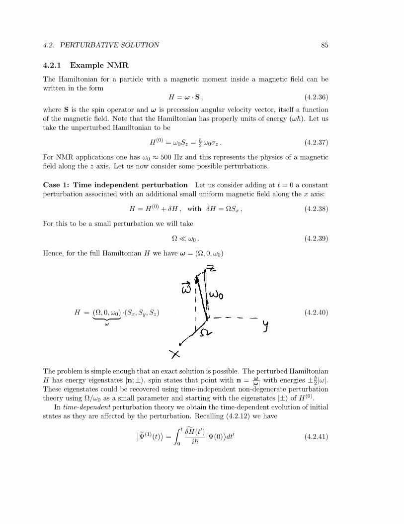
Hence, for the full Hamiltonian H we have ω = (Ω, 0, ω0)

H = (Ω, 0, ω0)︸︷︷︸ω

·(Sx, Sy, Sz) (4.2.40)

The problem is simple enough that an exact solution is possible. The perturbed HamiltonianH has energy eigenstates |n;±〉, spin states that point with n = ω

|ω| with energies ±~2 |ω|.

These eigenstates could be recovered using time-independent non-degenerate perturbationtheory using Ω/ω0 as a small parameter and starting with the eigenstates |±〉 of H(0).

In time-dependent perturbation theory we obtain the time-dependent evolution of initialstates as they are affected by the perturbation. Recalling (4.2.12) we have

∣∣Ψ(1)(t)⟩

=

∫ t

0

δH(t′)

i~∣∣Ψ(0)

⟩dt′ (4.2.41)


The calculation of δH requires a bit of computation. One quickly finds that

δH(t) = exp[iω0t

σz2

]ΩSx exp

[−iω0t

σz2

]= Ω

(Sx cosω0t− Sy sinω0t

). (4.2.42)

As a result we set:∣∣Ψ(1)(t)⟩

=Ω

i~

∫ t

0

(Sx cosω0t

′ − Sy sinω0t′) ∣∣Ψ(0)

⟩dt′

=1

i~Ω

ω0

[Sx sinω0t+

(cos(ω0t

′)− 1)Sy

] ∣∣Ψ(0)⟩. (4.2.43)

As expected, the result is first order in the small parameter Ω/ω0. Following (4.2.16) thetime-dependent state is, to first approximation

∣∣Ψ(t)⟩

= exp[−iω0t

σz2

](1 +

1

i~Ω

ω0

[Sx sinω0t+

(cos(ω0t

′)− 1)Sy

])|Ψ(0)〉

+O((Ω/ω0)2) .

(4.2.44)

Physically the solution is clear. The original spin state∣∣Ψ(0)

⟩precesses about the direction

of ω with angular velocity ω.

Case 2: Time dependent perturbation. Suppose that to the original Hamiltonian weadd the effect of a rotating magnetic field, rotating with the same angular velocity ω0 thatcorresponds to the Larmor frequency of the original Hamiltonian:

δH(t) = Ω(Sx cosω0t+ Sy sinω0t

). (4.2.45)

To compute the perturbation δH we can use (4.2.42) with t replaced by −t so that theright-hand side of this equation is proportional to δH:

exp[−iω0t

σz2

]ΩSx exp

[iω0t

σz2

]= Ω

(Sx cosω0t+ Sy sinω0t

). (4.2.46)

Moving the exponentials on the left-hand side to the right-hand side we find

ΩSx = exp[iω0t

σz2

]Ω(Sx cosω0t+ Sy sinω0t

)exp

[−iω0t

σz2

]. (4.2.47)

The right-hand side is, by definition, δH. Thus we have shown that

δH(t) = ΩSx , (4.2.48)

is in fact a time-independent Hamiltonian. This means that the Schrodinger equation for∣∣Ψ⟩ is immediately solved

∣∣Ψ(t)⟩

= exp

[−i δHt

~

]∣∣Ψ(0)⟩

= exp

[−iΩSx t

~

]∣∣Ψ(0)⟩. (4.2.49)

4.3. FERMI’S GOLDEN RULE 87

The complete and exact answer is therefore

∣∣Ψ(t)⟩

= exp[− iH

(0)t

~

]∣∣Ψ(t)⟩

= exp[−iω0t

σz2

]exp

[−iΩtσx

2

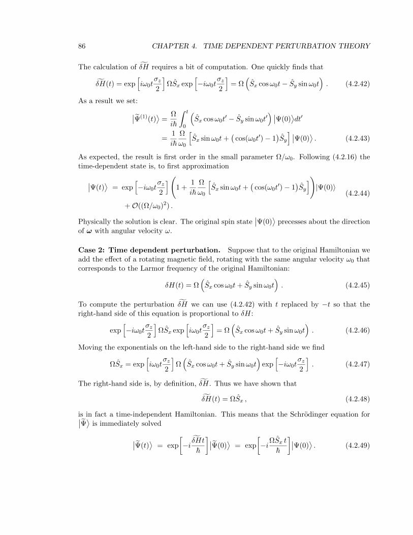
] ∣∣Ψ(0)⟩. (4.2.50)

This is a much more non trivial motion! A spin originally aligned along z will spiral intothe x, y plane with angular velocity Ω.

4.3 Fermi’s Golden Rule

Let us now consider transitions where the initial state is part of a discrete spectrum but thefinal state is part of a continuum. The ionization of an atom is perhaps the most familiarexample: the initial state may be one of the discrete bound states of the atom while thefinal state includes a free electron a momentum eigenstate that is part of a continuum ofnon-normalizable states.

As we will see, while the probability of transition between discrete states exhibits pe-riodic dependence in time, if the final state is part of a continuum an integral over finalstates is needed and the result is a transition probability linear in time. To such probabilityfunction we will be able to associate a transition rate. The final answer for the transitionrate is given by Fermi’s Golden Rule.

We will consider two different cases in full detail:

1. Constant perturbations. In this case the perturbation, called V turns on at t = 0 butit is otherwise time independent:

H =

H(0) , for t ≤ 0 ,

H(0) + V for t > 0 .(4.3.1)

This situation is relevant for the phenomenon of auto-ionization, where an internaltransition in the atom is accompanied by the ejection of an electron.


2. Harmonic perturbations. In this case the time dependence of the perturbation δH isperiodic, namely,

H(t) = H(0) + δH(t) , (4.3.2)

with

δH(t) =

0 , for t ≤ 0 ,

2H ′ cosωt , for t > 0 .(4.3.3)

Note the factor of two entering the definition of δH in terms of the time independentH ′. This situation is relevant to the interaction of electromagnetic fields with atoms.

Before starting with the analysis of these two cases let us consider the way to dealwith continuum states, as the final states in the transition will belong to a continuum.The fact is that we need to be able to count the states in the continuuum, so we willreplace infinite space by a very large cubic box of side length L and we will impose periodicboundary conditions on the wavefunctions. The result will be a discrete spectrum wherethe separation between the states can be made arbitrarily small, thus simulating accuratelya continuum in the limit L → ∞. If the states are energetic enough and the potential isshort range, momentum eigenstates are a good representation of the continuum.

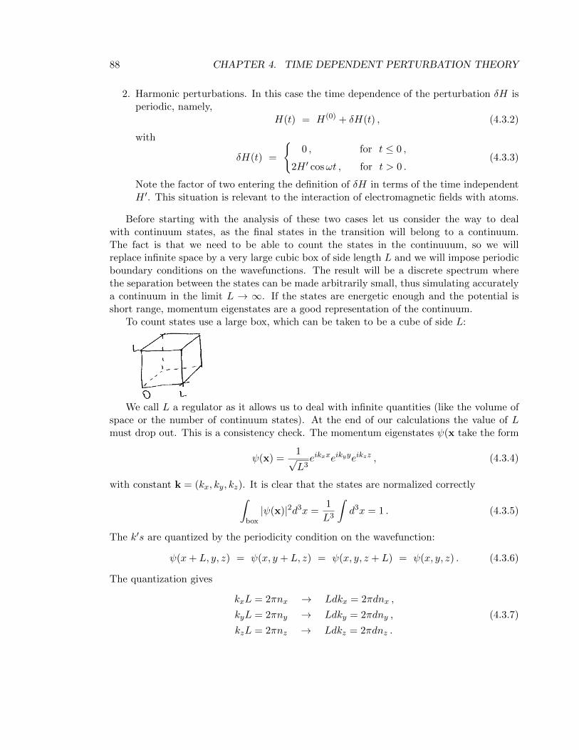
To count states use a large box, which can be taken to be a cube of side L:

We call L a regulator as it allows us to deal with infinite quantities (like the volume ofspace or the number of continuum states). At the end of our calculations the value of Lmust drop out. This is a consistency check. The momentum eigenstates ψ(x take the form

ψ(x) =1√L3eikxxeikyyeikzz , (4.3.4)

with constant k = (kx, ky, kz). It is clear that the states are normalized correctly∫box|ψ(x)|2d3x =

1

L3

∫d3x = 1 . (4.3.5)

The k′s are quantized by the periodicity condition on the wavefunction:

ψ(x+ L, y, z) = ψ(x, y + L, z) = ψ(x, y, z + L) = ψ(x, y, z) . (4.3.6)

The quantization gives

kxL = 2πnx → Ldkx = 2πdnx ,

kyL = 2πny → Ldky = 2πdny ,

kzL = 2πnz → Ldkz = 2πdnz .

(4.3.7)


Define ∆N as the total number of states within the little cubic volume element d3k. Itfollows from (4.3.7) that we have

∆N ≡ dnx dny dnz =

(L

2π

)3

d3k . (4.3.8)

Note that ∆N only depends on d3k and not on k itself: the density of states is constant inmomentum space.

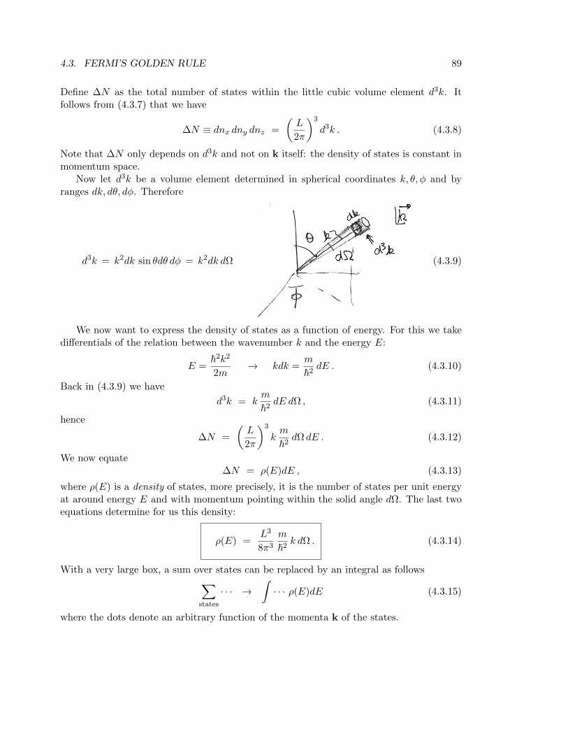
Now let d3k be a volume element determined in spherical coordinates k, θ, φ and byranges dk, dθ, dφ. Therefore

d3k = k2dk sin θdθ dφ = k2dk dΩ (4.3.9)

We now want to express the density of states as a function of energy. For this we takedifferentials of the relation between the wavenumber k and the energy E:

E =~2k2

2m→ kdk =

m

~2dE . (4.3.10)

Back in (4.3.9) we have

d3k = km

~2dE dΩ , (4.3.11)

hence

∆N =

(L

2π

)3

km

~2dΩ dE . (4.3.12)

We now equate∆N = ρ(E)dE , (4.3.13)

where ρ(E) is a density of states, more precisely, it is the number of states per unit energyat around energy E and with momentum pointing within the solid angle dΩ. The last twoequations determine for us this density:

ρ(E) =L3

8π3

m

~2k dΩ . (4.3.14)

With a very large box, a sum over states can be replaced by an integral as follows∑states

· · · →∫· · · ρ(E)dE (4.3.15)

where the dots denote an arbitrary function of the momenta k of the states.


4.3.1 Constant transitions.

The Hamiltonian, as given in (4.3.1) takes the form

H =

H(0) for t ≤ 0

H(0) + V for t > 0 .(4.3.16)

We thus identify δH(t) = V for t ≥ 0. Recalling the formula (4.2.33) for transition ampli-tudes to first order in perturbation theory we have

c(1)m (t) =

∑n

∫ t

0dt′eiωmnt

′ Vmni~

cn(0) . (4.3.17)

To represent an initial state i at = 0 we take cn(0) = δn,i. For a transition to a final statef at time t0 we set m = f and we have an integral that is easily performed:

c(1)f (t0) =

1

i~

∫ t0

0Vfi e

iωfi t′dt′ =

Vfii~

eiωfi t′

iωfi

∣∣∣∣∣t0

0

(4.3.18)

Evaluating the limits and simplifying

c(1)f (t0) =

VfiEf − Ei

(1− eiωfi t0

)=Vfi e

iωfit0/2

Ef − Ei(−2i) sin

(ωfi t

0

2

). (4.3.19)

The transition probability to go from i at t = 0 to f at t = t0 is then |c(1)f (t0)|2 and is

therefore

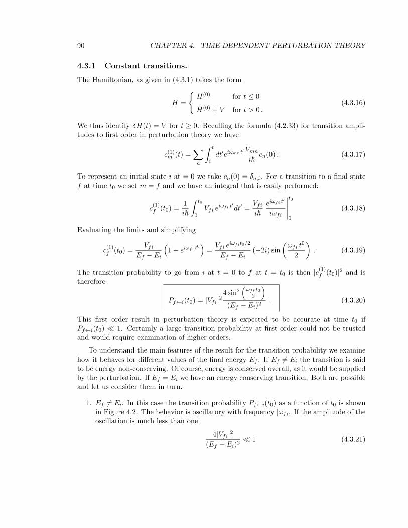
Pf←i(t0) = |Vfi|24 sin2

(ωfi t0

2

)(Ef − Ei)2

. (4.3.20)

This first order result in perturbation theory is expected to be accurate at time t0 ifPf←i(t0) 1. Certainly a large transition probability at first order could not be trustedand would require examination of higher orders.

To understand the main features of the result for the transition probability we examinehow it behaves for different values of the final energy Ef . If Ef 6= Ei the transition is saidto be energy non-conserving. Of course, energy is conserved overall, as it would be suppliedby the perturbation. If Ef = Ei we have an energy conserving transition. Both are possibleand let us consider them in turn.

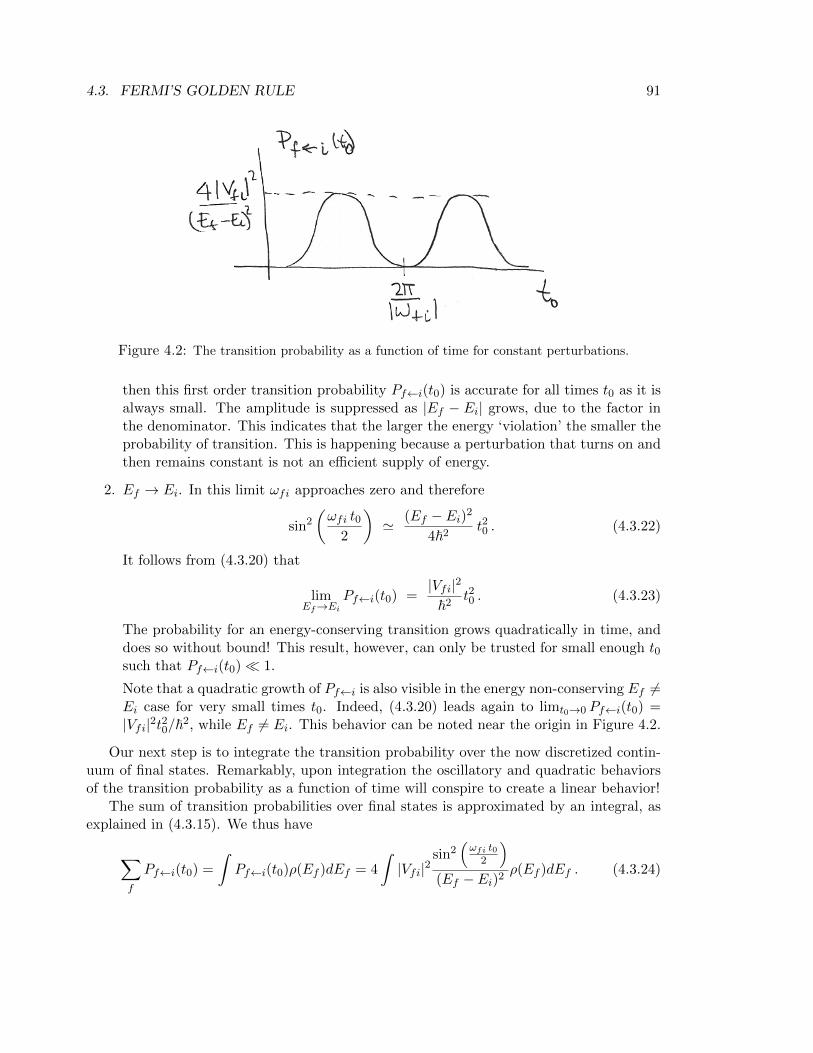
1. Ef 6= Ei. In this case the transition probability Pf←i(t0) as a function of t0 is shownin Figure 4.2. The behavior is oscillatory with frequency |ωfi. If the amplitude of theoscillation is much less than one

4|Vfi|2

(Ef − Ei)2 1 (4.3.21)


Figure 4.2: The transition probability as a function of time for constant perturbations.

then this first order transition probability Pf←i(t0) is accurate for all times t0 as it isalways small. The amplitude is suppressed as |Ef − Ei| grows, due to the factor inthe denominator. This indicates that the larger the energy ‘violation’ the smaller theprobability of transition. This is happening because a perturbation that turns on andthen remains constant is not an efficient supply of energy.

2. Ef → Ei. In this limit ωfi approaches zero and therefore

sin2

(ωfi t0

2

)'

(Ef − Ei)2

4~2t20 . (4.3.22)

It follows from (4.3.20) that

limEf→Ei

Pf←i(t0) =|Vfi|2

~2t20 . (4.3.23)

The probability for an energy-conserving transition grows quadratically in time, anddoes so without bound! This result, however, can only be trusted for small enough t0such that Pf←i(t0) 1.

Note that a quadratic growth of Pf←i is also visible in the energy non-conserving Ef 6=Ei case for very small times t0. Indeed, (4.3.20) leads again to limt0→0 Pf←i(t0) =|Vfi|2t20/~2, while Ef 6= Ei. This behavior can be noted near the origin in Figure 4.2.

Our next step is to integrate the transition probability over the now discretized contin-uum of final states. Remarkably, upon integration the oscillatory and quadratic behaviorsof the transition probability as a function of time will conspire to create a linear behavior!

The sum of transition probabilities over final states is approximated by an integral, asexplained in (4.3.15). We thus have

∑f

Pf←i(t0) =

∫Pf←i(t0)ρ(Ef )dEf = 4

∫|Vfi|2

sin2(ωfi t0

2

)(Ef − Ei)2

ρ(Ef )dEf . (4.3.24)


We have noted that Pf←i in the above integrand is suppressed as |Ef −Ei| becomes large.We therefore expect that the bulk of the contribution to the integral will occur for a narrowrange ∆Ef of Ef near Ei. Let us assume now that |Vfi|2 and ρ(Ef ) are slow varyingand therefore approximately constant over the narrow interval Ef (we will re-examine thisassumption below). If this is the case we can evaluate them for Ef set equal to Ei and takethem out of the integrand to find∑

f

Pf←i(t0) =4|Vfi|2

~2ρ(Ef = Ei) · I(t0) , (4.3.25)

where the integral I(t0) is given by

I(t0) ≡∫

1

ω2fi

sin2

(ωfi t0

2

)dEf = ~

∫sin2

(ωfi t0

2

)dωfiω2fi

. (4.3.26)

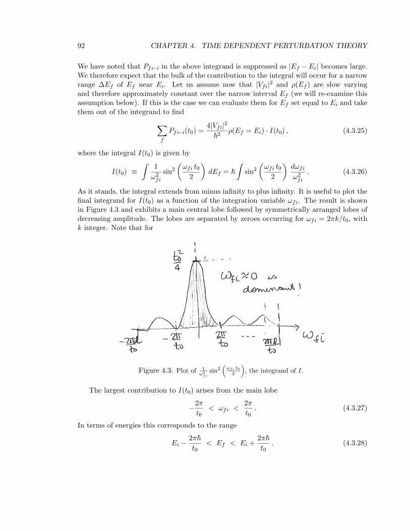
As it stands, the integral extends from minus infinity to plus infinity. It is useful to plot thefinal integrand for I(t0) as a function of the integration variable ωfi. The result is shownin Figure 4.3 and exhibits a main central lobe followed by symmetrically arranged lobes ofdecreasing amplitude. The lobes are separated by zeroes occurring for ωfi = 2πk/t0, withk integer. Note that for

Figure 4.3: Plot of 1ω2

fisin2

(ωfi t0

2

), the integrand of I.

The largest contribution to I(t0) arises from the main lobe

−2π

t0< ωfi <

2π

t0. (4.3.27)

In terms of energies this corresponds to the range

Ei −2π~t0

< Ef < Ei +2π~t0

. (4.3.28)


We need this range to be a narrow, thus t0 must be sufficiently large. The narrownessis required to justify our taking of the density of states ρ(E) and the matrix element |Vfi|2out of the integral. If we want to include more lobes this is can be made consistent with anarrow range of energies by making t0 larger.

The linear dependence of I(t0) as a function of t0 is intuitively appreciated by noticingthat the height of the main lobe is proportional to t20 and its width is proportional to 1/t0.In fact, the linear dependence is a simple mathematical fact made manifest by a change ofvariables. Letting

u =ωfit0

2=⇒ du =

t02dωfi , (4.3.29)

so that

I(t0) =2~t0

∫ ∞−∞

sin2 u

u2 · 4t20

=~t02

∫ ∞−∞

sin2 u

u2, (4.3.30)

making the linear dependence in t0 manifest. The remaining integral evaluates to π and wethus get

I(t0) = π2 ~t0 . (4.3.31)

Had restricted the integral to the main lobe, concerned that the density of states and matrixelements would vary over larger ranges, we would have gotten 90% of the total contribution.Including the next two lobes, one to the left and one to the right, brings the result up to95% of the total contribution. By the time we include ten or more lobes on each side weare getting 99% of the answer. For sufficiently large t0 is is still a narrow range.

Having determined the value of the integral I(t0) we can substitute back into our ex-pression for the transition probability (4.3.26). Replacing t0 by t

∑k

Pk←i(t) =4|Vfi|2

~2ρ(Ef )

π

2~t =

2π

~|Vfi|2ρ(Ef ) t . (4.3.32)

This holds, as discussed before, for sufficiently large t. Of course t cannot be too large as itwould make the transition probability large and unreliable. The linear dependence of thetransition probability implies we can define a transition rate w, or probability of transitionper unit time, by dividing the transition probability by t:

w ≡ 1

t

∑f

Pf←i(t) . (4.3.33)

This finally gives us Fermi’s golden rule for constant perturbations:

Fermi’s golden rule: w =2π

~|Vfi|2ρ(Ef ) , Ef = Ei . (4.3.34)

Not only is the density of states evaluated at the energy Ei, the matrix element Vfi is alsoevaluated at the energy Ei and other observables of the final state, like the momentum. In


this version of the golden rule the integration over final states has been performed. Theunits are manifestly right: |Vfi|2 has units of energy squared, ρ has units of one over energy,and with an ~ in the denominator the whole expression has units of one over time, asappropriate for a rate. We can also see that the dependence of w on the size-of-the-boxregulator L disappears: The matrix element

Vfi = 〈f |V |i〉 ∼ L−3/2 , (4.3.35)

because the final state wavefunction has such dependence (see (4.3.4)). Then the L depen-dence in |Vfi|2 ∼ L−3 cancels with the L dependence of the density of states ρ ∼ L3, notedin (4.3.14).

Let us summarize the approximations used to derive the golden rule. We have twoconditions that must hold simultaneously:

1. We assumed that t0 is large enough so that the energy range

Ei − k2π~t0

< Ef < Ei + k2π~t0

, (4.3.36)

with k some small integer, is narrow enough that ρ(E) and |Vfi|2 are approximatelyconstant over this range. This allowed us to take them out of the integral simplifyinggreatly the problem and making a complete evaluation possible.

2. We cannot allow t0 to be arbitrarily large. As we have∑f

Pf←i(t0) = w t0 , (4.3.37)

we must keep wt0 1 for our first order calculation to be accurate.

Can the two conditions on t0 be satisfied? There is no problem if the perturbation canbe made small enough: indeed, suppose condition 1 is satisfied for some suitable t0 butcondition 2 is not. Then we can make the perturbation V smaller making w small enoughthat the second condition is satisfied. In practice, in specific problems, one could do thefollowing check. First compute w assuming the golden rule. Then fix t0 such that wt0 isvery small, say equal to 0.01. Then check that over the range ∼ ~/t0 the density of statesand the matrix elements are roughly constant. If this works out the approximation shouldbe very good!

Helium atom and autoionization. The helium has two protons (Z = 2) and twoelectrons. Let H(0) be the Hamiltonian for this system ignoring the the Coulomb repulsionbetween the electrons:

H(0) =p2

1

2m− e2

r1+

p22

2m− e2

r2. (4.3.38)


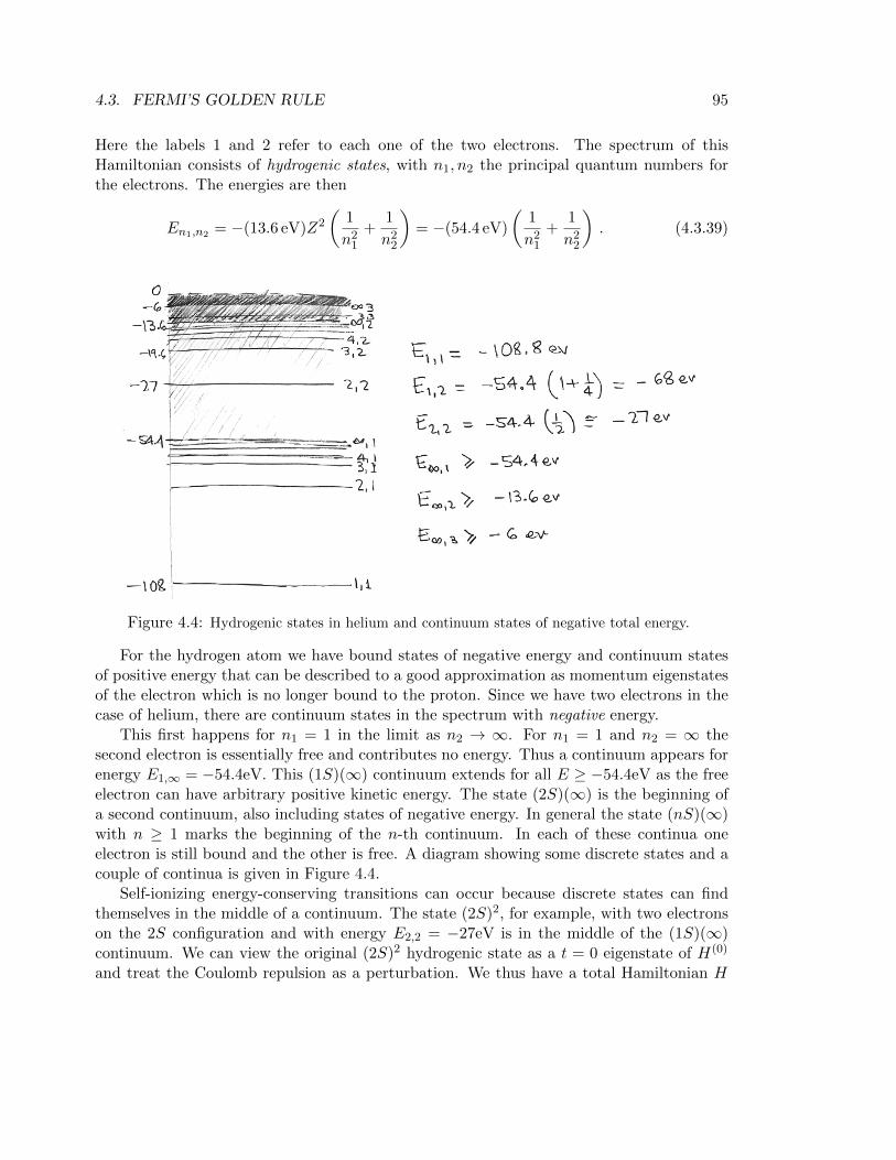
Here the labels 1 and 2 refer to each one of the two electrons. The spectrum of thisHamiltonian consists of hydrogenic states, with n1, n2 the principal quantum numbers forthe electrons. The energies are then

En1,n2 = −(13.6 eV)Z2

(1

n21

+1

n22

)= −(54.4 eV)

(1

n21

+1

n22

). (4.3.39)

Figure 4.4: Hydrogenic states in helium and continuum states of negative total energy.

For the hydrogen atom we have bound states of negative energy and continuum statesof positive energy that can be described to a good approximation as momentum eigenstatesof the electron which is no longer bound to the proton. Since we have two electrons in thecase of helium, there are continuum states in the spectrum with negative energy.

This first happens for n1 = 1 in the limit as n2 → ∞. For n1 = 1 and n2 = ∞ thesecond electron is essentially free and contributes no energy. Thus a continuum appears forenergy E1,∞ = −54.4eV. This (1S)(∞) continuum extends for all E ≥ −54.4eV as the freeelectron can have arbitrary positive kinetic energy. The state (2S)(∞) is the beginning ofa second continuum, also including states of negative energy. In general the state (nS)(∞)with n ≥ 1 marks the beginning of the n-th continuum. In each of these continua oneelectron is still bound and the other is free. A diagram showing some discrete states and acouple of continua is given in Figure 4.4.

Self-ionizing energy-conserving transitions can occur because discrete states can findthemselves in the middle of a continuum. The state (2S)2, for example, with two electronson the 2S configuration and with energy E2,2 = −27eV is in the middle of the (1S)(∞)continuum. We can view the original (2S)2 hydrogenic state as a t = 0 eigenstate of H(0)

and treat the Coulomb repulsion as a perturbation. We thus have a total Hamiltonian H


that takes the form

H = H(0) + V , V =e2

|r1 − r2|. (4.3.40)

The perturbation V produces “auto-ionizing” Auger transitions to the continuum. We havea transition from a state with energy E2,2 = −27eV to a state of one bound electron withenergy −54.4eV and one free electron with kinetic energy of 27eV. That final state is partof a continuum. Radiative transitions from (2S)2 to 1S2S, with photo-emission, are in facta lot less likely than auto-ionizing transitions!

We will not do the quantitative analysis required to determine lifetime of the (2S)2 state.In general auto-ionization is a process in which an atom or a molecule in an excited statespontaneously emits one of the outer-shell electrons. Auto-ionizing states are in generalshort lived. Auger transitions are auto-ionization processes in which the filling of an innershell vacancy is accompanied by the emission of an electron. Our example of the (2S)2

state is an Auger transition. Molecules can have auto ionizing Rydberg states, in which thelittle energy needed to remove the Rydberg electron is supplied by a vibrational excitationof the molecule.

4.3.2 Harmonic Perturbation

It is now time to consider the case when the perturbation is harmonic. We will be ableto derive a similar looking Fermi golden rule for the transition rate. The most importantdifference is that now the transitions are of two types. They involve either absorption ofenergy or a release of energy. In both cases that energy (absorbed or released) is equal to~ω where ω is the frequency of the perturbation.

As indicated in (4.3.3) we have

H(t) = H(0) + δH(t) , (4.3.41)

where the perturbation δH(t) takes the form

δH(t) =

0 , for t ≤ 0 ,

2H ′ cosωt , for t > 0 .(4.3.42)

Here ω > 0 and H ′ is some time independent Hamiltonian. The inclusion of an extra factorof two in the relation between δH and H ′ is convenient because it results in a golden ruledoes not have additional factors of two compared to the case of constant transitions.

We again consider transitions from an initial state i to a final state f . The transitionamplitude this time From (4.2.33)

c(1)f (t)) =

1

i~

∫ t0

0dt′ eiωfit

′δHfi(t

′) . (4.3.43)


Using the explicit form of δH the integral can be done explicitly

c(1)f (t0) =

1

i~

∫ t0

0eiωfit

′2H ′fi cosωt′dt′

=H ′fii~

∫ t0

0

(ei(ωfi+ω)t′ + ei(ωfi−ω)t′

)dt′

= −H ′fi~

[ei(ωfi+ω)t0 − 1

ωfi + ω+ei(ωfi−ω)t0 − 1

ωfi − ω

].

(4.3.44)

Comments:

• The amplitude takes the form of a factor multiplying the sum of two terms, each one afraction. As t0 → 0 each fraction goes to it0. For finite t0, which is our case of interest,each numerator is a complex number of bounded absolute value that oscillates in timefrom zero up to two. In comparing the two terms the relevant one is the one with thesmallest denominator.1

• The first term is relevant as ωfi + ω ≈ 0, that is, when there are states at energyEf = Ei − ~ω. This is “stimulated emission”, the source has stimulated a transitionin which energy ~ω is released.

• The second term relevant if ωfi − ω ≈ 0, that is, when there are states at energyEf = Ei + ~ω. Energy is transferred from the perturbation to the system, and wehave a process of “absorption”.

Both cases are of interest. Let us do the calculations for the case of absorption; theanswer for the case of spontaneous emission will be completely analogous. We take i to bea discrete state, possibly bound, and f to be a state in the continuum at the higher energyEf ≈ Ei + ~ω. Since ωfi ' ω, the second term in the last line of (4.3.44) is much moreimportant than the first. Keeping only the second term we have

c(1)f (t0) = −

H ′fi~ei2

(ωfi−ω)t0

ωfi − ω2i sin

(ωfi − ω

2t0

), (4.3.45)

and the transition probability is

Pf←i(t0) = |c(1)f (t0)|2 =

4|H ′fi|2

~2

sin2(ωfi−ω

2 t0

)(ωfi − ω)2

(4.3.46)

The transition probability is exactly the same as that for constant perturbations (see(4.3.20)) with V replaced by H ′ and ωfi replaced by ωfi − ω. The analysis that follows is

1This is like comparing two waves that are being superposed. The one with larger amplitude is morerelevant even though at some special times, as it crosses the value of zero, it is smaller than the other wave.


completely analogous to the previous one so we shall be brief. Summing over final stateswe have

∑k

Pk←i(t0) =

∫Pf←i ρ(Ef )dEf =

∫4|H ′fi|2

~2

sin2(ωfi−ω

2 t0

)(ωfi − ω)2

ρ(Ef )dEf . (4.3.47)

This time the main contribution comes from the region

−2π

t0< ωfi − ω <

2π

t0(4.3.48)

In terms of the final energy this is the band

Ei + ~ω − 2π~t0

< Ef < Ei + ~ω +2π~t0

(4.3.49)

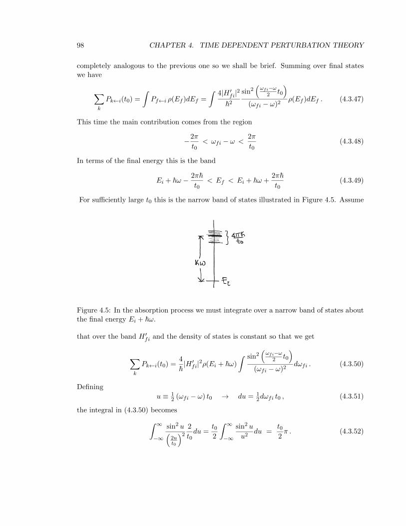
For sufficiently large t0 this is the narrow band of states illustrated in Figure 4.5. Assume

Figure 4.5: In the absorption process we must integrate over a narrow band of states aboutthe final energy Ei + ~ω.

that over the band H ′fi and the density of states is constant so that we get

∑k

Pk←i(t0) =4

~|H ′fi|2ρ(Ei + ~ω)

∫ sin2(ωfi−ω

2 t0

)(ωfi − ω)2

dωfi . (4.3.50)

Defining

u ≡ 12 (ωfi − ω) t0 → du = 1

2dωfi t0 , (4.3.51)

the integral in (4.3.50) becomes∫ ∞−∞

sin2 u(2ut0

)2

2

t0du =

t02

∫ ∞−∞

sin2 u

u2du =

t02π . (4.3.52)

4.4. IONIZATION OF HYDROGEN 99

Finally, the transition probability is∑k

Pk←i(t0) =2π

~|H ′fi|2ρ(Ei + ~ω) t0 . (4.3.53)

The transition rate w is finally given by

Fermi’s golden rule: w =2π

~ρ(Ef )|H ′fi|2 , Ef = Ei + ~ω . (4.3.54)

Here H ′(t) = 2H ′ cosωt. Equation (4.3.54) is known as Fermi’s golden rule for the case ofharmonic perturbations. For the case of spontaneous emission the only change required inthe above formula is Ef = Ei − ~ω.

4.4 Ionization of hydrogen

We aim to find the ionization rate for hydrogen when hit by the harmonically varyingelectric field of an electromagnetic wave. We assume the hydrogen atom has its electronon the ground state. In this ionization process a photon ejects the bound electron, whichbecomes free.

Let us first do a few estimates to understand the validity of the approximations that willbe required. If the electromagnetic field has frequency ω the incident photons have energy

Eγ = ~ω . (4.4.1)

The energy Ee and the magnitude k of the momentum of the ejected electron are given by

Ee =~2k2

2m= Eγ −Ry , (4.4.2)

where the Rydberg Ry is the magnitude of the energy of the ground state:

2Ry =e2

a0=

~2

ma20

= α~ca0, Ry ' 13.6 eV . (4.4.3)

Inequalities

1. Any electromagnetic wave has spatial dependence. We can ignore the spatial depen-dence of the wave if the wavelength λ of the photon is much bigger than the Bohrradius a0:

λ

a0 1 . (4.4.4)

Such a condition puts an upper bound on the photon energy, since the more energeticphoton the smaller its wavelength. To bound the energy we first write

λ =2π

kγ=

2πc

ω=

2π~c~ω

, (4.4.5)


and then find

λ

a0=

2π

~ω~ca0

=4π

α

Ry~ω' 1722

Ry~ω

(4.4.6)

The inequality (4.4.4) then gives

~ω 1722Ry ' 23 keV (4.4.7)

2. For final states we would like to use free particle momentum eigenstates. This requiresthe ejected electron to be energetic enough not to be much effected by the Coulombfield. As a result, the photon to be energetic enough, and this constraint provides alower bound for its energy. We have

Ee = Eγ −Ry Ry → ~ω Ry . (4.4.8)

The two inequalities above imply

Ry ~ω 1722Ry . (4.4.9)

If consider that 1 10 we could take

140eV ≤ ~ω ≤ 2.3 keV . (4.4.10)

Note that even for the upper limit the electron is non relativistic: 2.3 keV mec2 ' 511keV.

Exercise: Determine ka0 in terms of ~ω and Ry.Solution:

~2k2

2m= ~ω −Ry = Ry

(~ωRy− 1

)=

~2

2ma20

(~ωRy− 1

)(4.4.11)

k2a20 =

~ωRy− 1 → ka0 =

√~ωRy− 1 . (4.4.12)

This is the desired result. In the range of (4.4.10) we have

3 ≤ ka0 ≤ 13 . (4.4.13)

Calculating the matrix element. Our perturbation Hamiltonian is

δH = −eΦ , (4.4.14)

where Φ is the electric scalar potential. Let the electric field at the atom be polarized inthe z direction

E(t) = E(t)z = 2E0 cosωt z (4.4.15)


The associated scalar potential isΦ = −E(t)z , (4.4.16)

and therefore

δH = eE(t)z = eE(t)r cos θ = 2 eE0r cos θ︸︷︷︸H′

cosωt ≡ 2H ′ cosωt (4.4.17)

We have thus identified, in our notation,

H ′ = eE0r cos θ . (4.4.18)

We want to compute the matrix element between an initial state |i〉 that is the ground stateof hydrogen, and a final state |f〉 which is an electron plane wave with momentum ke. Theassociated wavefunctions are

Final state: uk(x) =1

L3/2eik·r (4.4.19)

Initial state: ψ0(r) =1√πa3

0

e− ra0 (4.4.20)

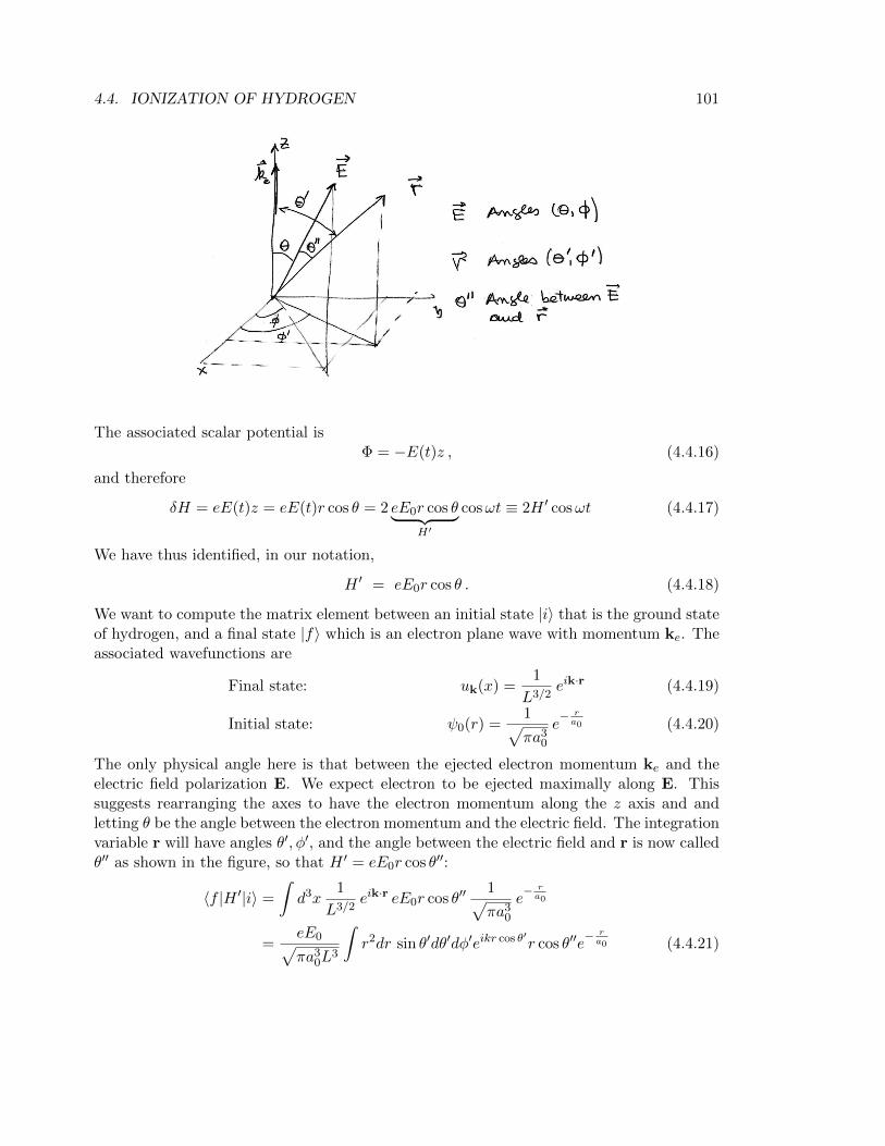
The only physical angle here is that between the ejected electron momentum ke and theelectric field polarization E. We expect electron to be ejected maximally along E. Thissuggests rearranging the axes to have the electron momentum along the z axis and andletting θ be the angle between the electron momentum and the electric field. The integrationvariable r will have angles θ′, φ′, and the angle between the electric field and r is now calledθ′′ as shown in the figure, so that H ′ = eE0r cos θ′′:

〈f |H ′|i〉 =

∫d3x

1

L3/2eik·r eE0r cos θ′′

1√πa3

0

e− ra0

=eE0√πa3

0L3

∫r2dr sin θ′dθ′dφ′eikr cos θ′r cos θ′′e

− ra0 (4.4.21)


The main complication with doing the integral is the factor cos θ′′. The dot product of unitvectors along E and n is cos θ′′:

cos θ′′ = (sin θ cosφ)(sin θ′ cosφ′) + (sin θ sinφ)(sin θ′ sinφ′) + cos θ cos θ′

= sin θ sin θ′ cos(φ− φ′) + cos θ cos θ′ (4.4.22)

Since the following integral vanishes∫dφ′ cos(φ− φ′) = 0 (4.4.23)

the first term in the expression for cos θ′′ will vanish upon φ′ integration. We therefore canreplace cos θ′′ → cos θ cos θ′ to find

〈f |H ′|i〉 =eE0√πa3

0L3

∫r3dr sin θ′dθ′dφ′eikr cos θ′ cos θ cos θ′e

− ra0

=eE0√πa3

0L3(cos θ)(2π)

∫r3dr e

− ra0

∫ 1

−1d(cos θ′) cos θ′eikr cos θ′ (4.4.24)

Now let r = a0u and do the radial integration:

〈f |H ′|i〉 =eE0√πa3

0L32π cos θa4

0

∫ 1

−1d(cos θ′) cos θ′

∫u3du e−u(1+ika0 cos θ′)

=eE0√πa3

0L32π cos θa4

0

∫ 1

−1d(cos θ′) cos θ′

3!

(1 + ika0 cos θ′)4. (4.4.25)

Writing x = cos θ′ the angular integral is not complicated:

〈f |H ′|i〉 =eE0√πa3

0L3

2π cos θa40

3!

(ika0)4

∫ 1

−1

x(x+ 1

ika0

)4dx

=eE0√πa3

0L3

2π cos θa40

3!

(ika0)4

8(

1ika0

)3(

1 + 1k2a20

)3

= −i32πeE0a0√πa3

0L3

ka40

(1 + k2a20)3

cos θ (4.4.26)

Hence, with a little rearrangement

〈f |H ′|i〉 = −i32√π (eE0a0)

ka40√

a30L

3

1

(1 + k2a20)3

cos θ . (4.4.27)

The above matrix element has the units of (eE0a), which is energy. This is as expected.Squaring we find

|H ′fi|2 = 1024π (eE0a)2 k2a5

0

L3

cos2 θ

(1 + k2a20)6

(4.4.28)


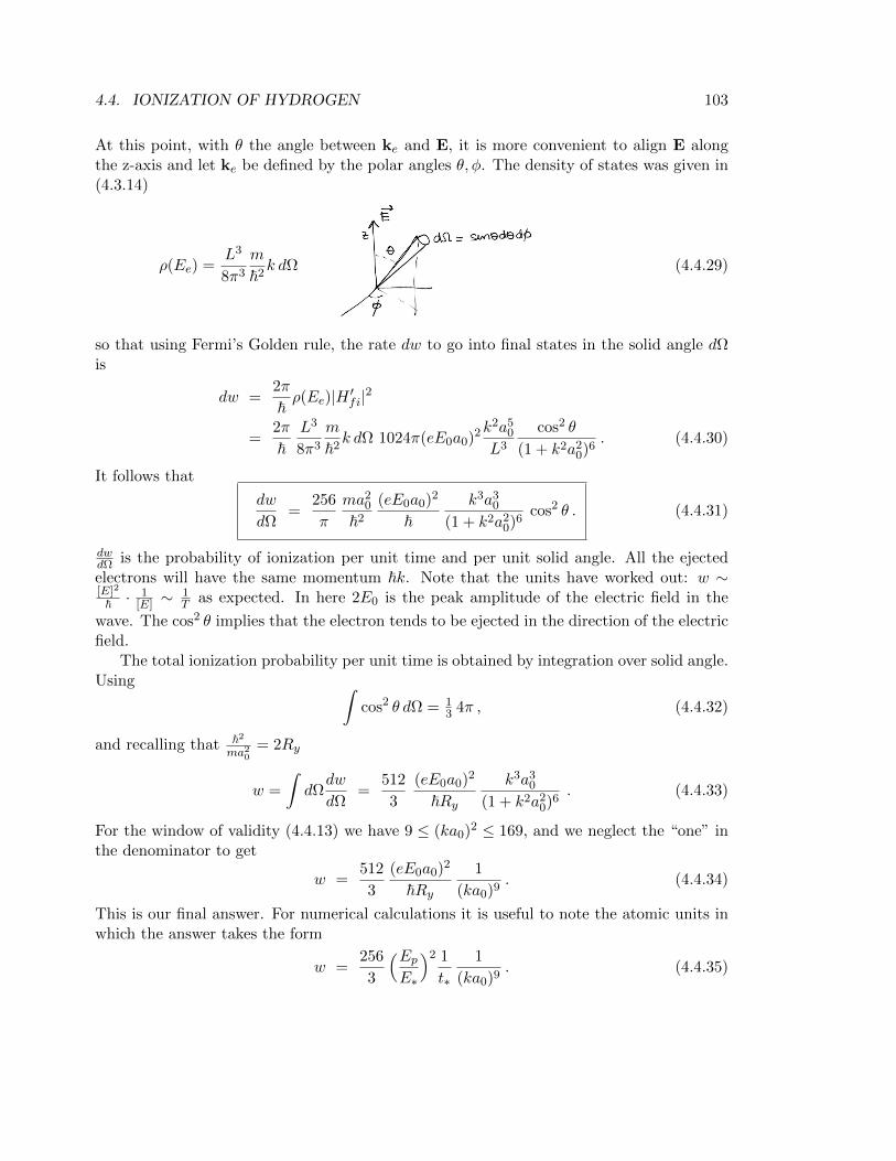
At this point, with θ the angle between ke and E, it is more convenient to align E alongthe z-axis and let ke be defined by the polar angles θ, φ. The density of states was given in(4.3.14)

ρ(Ee) =L3

8π3

m

~2k dΩ (4.4.29)

so that using Fermi’s Golden rule, the rate dw to go into final states in the solid angle dΩis

dw =2π

~ρ(Ee)|H ′fi|2

=2π

~L3

8π3

m

~2k dΩ 1024π(eE0a0)2k

2a50

L3

cos2 θ

(1 + k2a20)6

. (4.4.30)

It follows that

dw

dΩ=

256

π

ma20

~2

(eE0a0)2

~k3a3

0

(1 + k2a20)6

cos2 θ . (4.4.31)

dwdΩ is the probability of ionization per unit time and per unit solid angle. All the ejectedelectrons will have the same momentum ~k. Note that the units have worked out: w ∼[E]2

~ ·1

[E] ∼1T as expected. In here 2E0 is the peak amplitude of the electric field in the

wave. The cos2 θ implies that the electron tends to be ejected in the direction of the electricfield.

The total ionization probability per unit time is obtained by integration over solid angle.Using ∫

cos2 θ dΩ = 13 4π , (4.4.32)

and recalling that ~2ma20

= 2Ry

w =

∫dΩ

dw

dΩ=

512

3

(eE0a0)2

~Ryk3a3

0

(1 + k2a20)6

. (4.4.33)

For the window of validity (4.4.13) we have 9 ≤ (ka0)2 ≤ 169, and we neglect the “one” inthe denominator to get

w =512

3

(eE0a0)2

~Ry1

(ka0)9. (4.4.34)

This is our final answer. For numerical calculations it is useful to note the atomic units inwhich the answer takes the form

w =256

3

(EpE∗

)2 1

t∗

1

(ka0)9. (4.4.35)


Here Ep = 2E0 is the peak amplitude of the electric field. Moreover, the atomic electricfield E∗ and the atomic time t∗ are given by

E∗ =2Ryea0

=e

a20

= 5.14× 1011V/m

t∗ =a0

αc= 2.42× 10−17 sec.

(4.4.36)

Note that E∗ is the electric field of a proton at a distance a0 while t∗ is the time it takesthe electron to travel a distance a0 at the velocity αc in the ground state. A laser intensityof 3.55× 1016W/cm2 has an peak electric field of magnitude E∗.

4.5 Light and atoms

4.5.1 Absorption and stimulated emission

The physical problem we are trying to solve consists of a collection of atoms with twopossible energy levels interacting with light at a temperature T . We want to understandthe processes of absorption and emission of radiation and how they can produce thermalequilibrium.

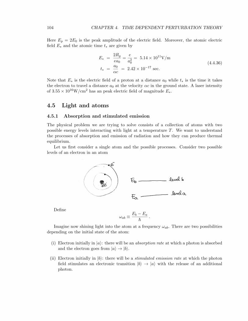
Let us first consider a single atom and the possible processes. Consider two possiblelevels of an electron in an atom

Define

ωab ≡Eb − Ea

~.

Imagine now shining light into the atom at a frequency ωab. There are two possibilitiesdepending on the initial state of the atom:

(i) Electron initially in |a〉: there will be an absorption rate at which a photon is absorbedand the electron goes from |a〉 → |b〉.

(ii) Electron initially in |b〉: there will be a stimulated emission rate at which the photonfield stimulates an electronic transition |b〉 → |a〉 with the release of an additionalphoton.

4.5. LIGHT AND ATOMS 105

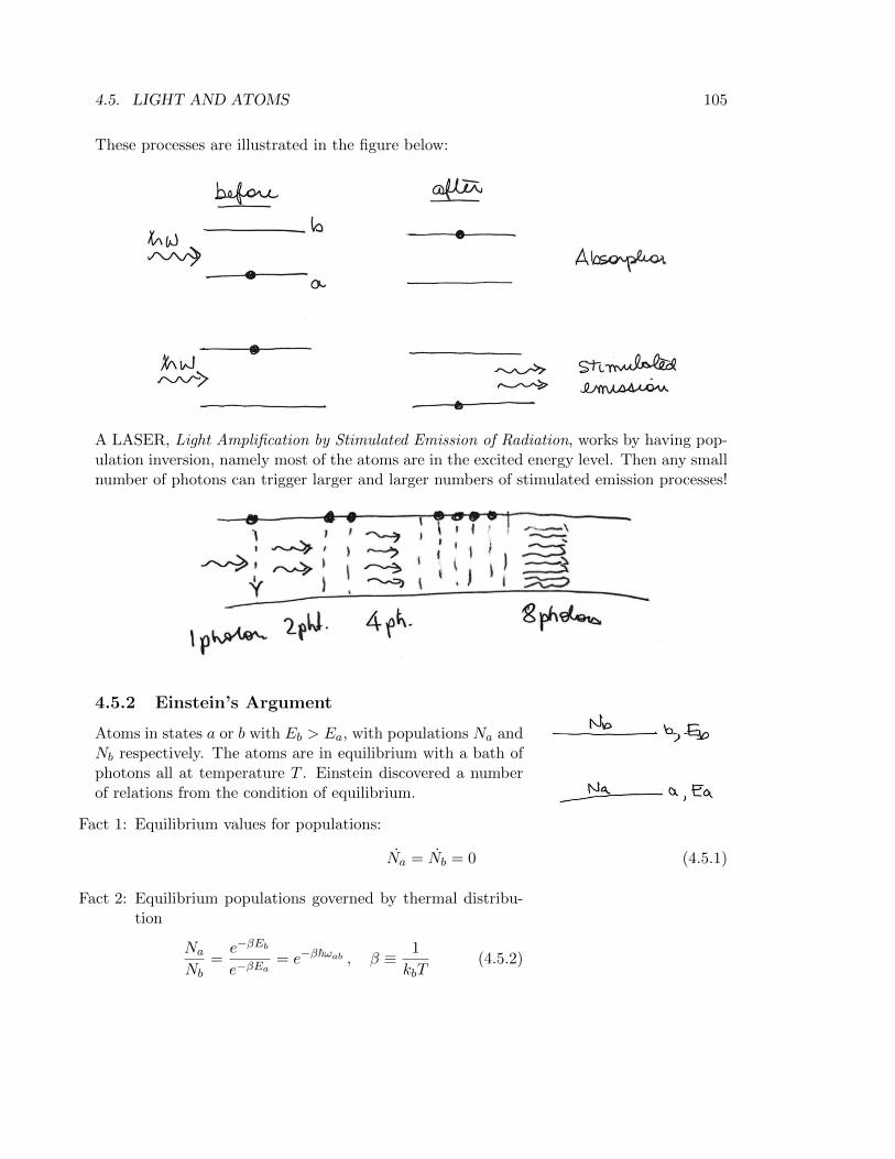
These processes are illustrated in the figure below:

A LASER, Light Amplification by Stimulated Emission of Radiation, works by having pop-ulation inversion, namely most of the atoms are in the excited energy level. Then any smallnumber of photons can trigger larger and larger numbers of stimulated emission processes!

4.5.2 Einstein’s Argument

Atoms in states a or b with Eb > Ea, with populations Na andNb respectively. The atoms are in equilibrium with a bath ofphotons all at temperature T . Einstein discovered a numberof relations from the condition of equilibrium.

Fact 1: Equilibrium values for populations:

Na = Nb = 0 (4.5.1)

Fact 2: Equilibrium populations governed by thermal distribu-tion

Na

Nb=e−βEb

e−βEa= e−β~ωab , β ≡ 1

kbT(4.5.2)


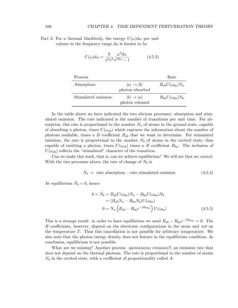
Fact 3: For a thermal blackbody, the energy U(ω)dω per unitvolume in the frequency range dω is known to be

U(ω)dω =~

π2c3

ω3dω

eβ~ω − 1(4.5.3)

Process Rate

Absorption: |a〉 → |b〉 BabU(ωba)Na

photon absorbed

Stimulated emission: |b〉 → |a〉 BbaU(ωba)Nb

photon released

In the table above we have indicated the two obvious processes: absorption and stim-ulated emission. The rate indicated is the number of transitions per unit time. For ab-sorption, this rate is proportional to the number Na of atoms in the ground state, capableof absorbing a photon, times U(ωab) which captures the information about the number ofphotons available, times a B coefficient Bab that we want to determine. For stimulatedemission, the rate is proportional to the number Nb of atoms in the excited state, thuscapable of emitting a photon, times U(ωab) times a B coefficient Bba. The inclusion ofU(ωab) reflects the “stimulated” character of the transition.

Can we make this work, that is, can we achieve equilibrium? We will see that we cannot.With the two processes above, the rate of change of Nb is

Nb = rate absorption− rate stimulated emission (4.5.4)

At equilibrium Nb = 0, hence

0 = Nb = BabU(ωba)Na −BbaU(ωba)Nb

= (BabNa −BbaNb)U(ωba)

0 = Na

(Bab −Bbae−β~ωba

)U(ωba) (4.5.5)

This is a strange result: in order to have equilibrium we need Bab − Bbae−β~ωba = 0. TheB coefficients, however, depend on the electronic configurations in the atom and not onthe temperature T . Thus this cancellation is not possible for arbitrary temperature. Wealso note that the photon energy density does not feature in the equilibrium condition. Inconclusion, equilibrium is not possible.

What are we missing? Another process: spontaneous emission!!, an emission rate thatdoes not depend on the thermal photons. The rate is proportional to the number of atomsNb in the excited state, with a coefficient of proportionality called A:


Process Rate

Spontaneous emission: |b〉 → |a〉 ANb

photon released

Reconsider now the equilibrium condition with this extra contribution to Nb:

0 = Nb = BabU(ωba)Na − BbaU(ωba)Nb − ANb

=⇒ A =

(Bab

Na

Nb−Bba

)U(ωba)

=⇒ U(ωba) =A

Bab

1

eβ~ωba − BbaBab

(4.5.6)

The equilibrium condition indeed gives some important constraint on U(ωab). But from Eq.(4.5.3) we know

U(ωba) =~ω3

ba

π2c3

1

eβ~ωba − 1(4.5.7)

Hence comparing the two equations we get

Bab = Bba andA

Bab=

~ω3ba

π2c3(4.5.8)

As we’ll see, we’ll be able to calculate Bab, but A is harder. Happily, thanks to (4.5.8), wecan obtain A from Bab.

Spontaneous emission does not care about U(ωba); the photons flying around. At adeep level one can think of spontaneous emission as stimulated emission due to vacuumfluctuation of the EM field.

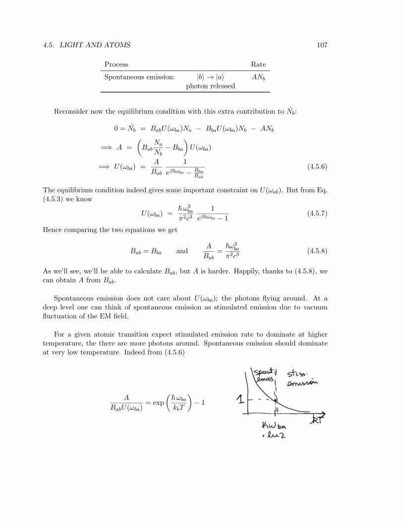
For a given atomic transition expect stimulated emission rate to dominate at highertemperature, the there are more photons around. Spontaneous emission should dominateat very low temperature. Indeed from (4.5.6)

A

BabU(ωba)= exp

(~ωbakbT

)− 1


4.5.3 Atom/light interaction

Focus on ~E field. Effects of ~B are weaker by O(vc

)∼ α. For optical frequencies λ ∼

4000− 8000 A and since a0 ' 0.5 A, we can ignore the spatial dependence of the field (evenfor ionization frequencies λ

a0∼ 1700)

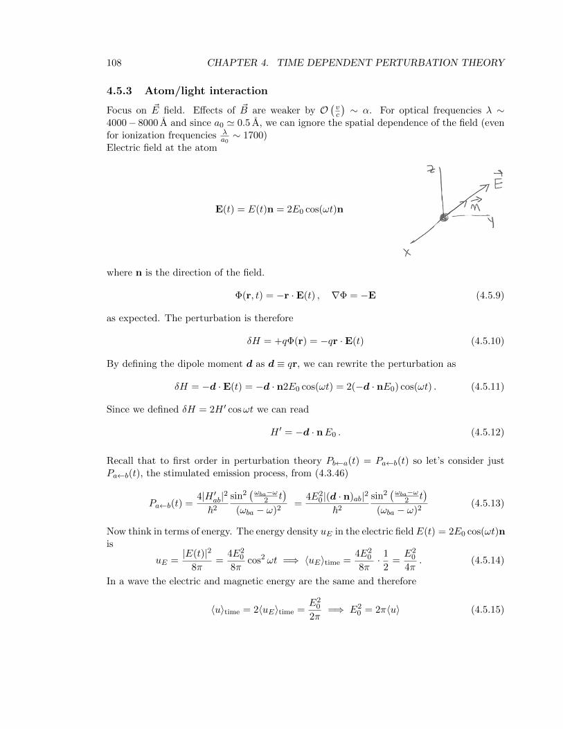
Electric field at the atom

E(t) = E(t)n = 2E0 cos(ωt)n

where n is the direction of the field.

Φ(r, t) = −r ·E(t) , ∇Φ = −E (4.5.9)

as expected. The perturbation is therefore

δH = +qΦ(r) = −qr ·E(t) (4.5.10)

By defining the dipole moment d as d ≡ qr, we can rewrite the perturbation as

δH = −d ·E(t) = −d · n2E0 cos(ωt) = 2(−d · nE0) cos(ωt) . (4.5.11)

Since we defined δH = 2H ′ cosωt we can read

H ′ = −d · nE0 . (4.5.12)

Recall that to first order in perturbation theory Pb←a(t) = Pa←b(t) so let’s consider justPa←b(t), the stimulated emission process, from (4.3.46)

Pa←b(t) =4|H ′ab|2

~2

sin2(ωba−ω

2 t)

(ωba − ω)2=

4E20 |(d · n)ab|2

~2

sin2(ωba−ω

2 t)

(ωba − ω)2(4.5.13)

Now think in terms of energy. The energy density uE in the electric field E(t) = 2E0 cos(ωt)nis

uE =|E(t)|2

8π=

4E20

8πcos2 ωt =⇒ 〈uE〉time =

4E20

8π· 1

2=E2

0

4π. (4.5.14)

In a wave the electric and magnetic energy are the same and therefore

〈u〉time = 2〈uE〉time =E2

0

2π=⇒ E2

0 = 2π〈u〉 (4.5.15)


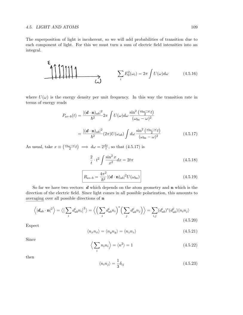
The superposition of light is incoherent, so we will add probabilities of transition due toeach component of light. For this we must turn a sum of electric field intensities into anintegral.

∑i

E20(ωi) = 2π

∫U(ω)dω (4.5.16)

where U(ω) is the energy density per unit frequency. In this way the transition rate interms of energy reads

Pa←b(t) =|(d · n)ab|2

~22π

∫U(ω)dω

sin2(ωba−ω

2 t)

(ωba − ω)2

=|(d · n)ab|2

~2(2π)U(ωab)

∫dω

sin2(ωba−ω

2 t)

(ωba − ω)2(4.5.17)

As usual, take x ≡(ωba−ω

2 t)

=⇒ dω = 2dxt , so that (4.5.17) is

2

t· t2∫

sin2 x

x2dx = 2tπ (4.5.18)

Ra←b =4π2

~2|(d · n)ab|2U(ωba) (4.5.19)

So far we have two vectors: d which depends on the atom geometry and n which is thedirection of the electric field. Since light comes in all possible polarization, this amounts toaveraging over all possible directions of n⟨

|dab · n|2⟩

=⟨∣∣∑

i

diabni∣∣2⟩ =

⟨(∑i

diabni

)∗(∑j

djabnj

)⟩=∑i,j

(diab)∗(djab)〈ninj〉

(4.5.20)Expect

〈nxnx〉 = 〈nyny〉 = 〈nznz〉 (4.5.21)

Since ⟨∑i

nini

⟩= 〈n2〉 = 1 (4.5.22)

then

〈ninj〉 =1

3δij (4.5.23)


⟨|dab · n|2

⟩=

1

3d∗ab · dab ≡

1

3|dab|2 (4.5.24)

This is the magnitude of a complex vector!

Ra←b =4π2

3~2|dab|2U(ωba) (4.5.25)

This is the transition probability per unit time for a single atom

Bab =4π2

3~2|dab|2 (4.5.26)

thus recalling (4.5.8)

A =~ω3

ba

π2c3Bab =

~ω3ba

π2c3

4π2

3~2|dab|2 (4.5.27)

hence we have that A, the transition probability per unit time for an atom to go from|b〉 → |a〉, is

A =4

3

ω3ba

~c3|dab|2 . (4.5.28)

The lifetime for the state is τ = 1A . The number N of particles decays exponentially in time

dN

dt= −AN =⇒ N(t) = e−At = N0e

−t/τ (4.5.29)

If there are various decay possibilities A1, A2, . . . , the transition rates add

Atot. = A1 +A2 + . . . and τ =1

Atot.(4.5.30)

4.5.4 Selection rules

(to be covered in recitation) Given two states |n`m〉 and |n′`′m′〉, when 〈n`m|r|n′`′m′〉 6= 0?One can learn that

〈n`m|z|n′`′m′〉 = 0 for m′ 6= m (4.5.31)

〈n`m|x|n′`′m′〉 = 〈n`m|y|n′`′m′〉 = 0 for m′ 6= m± 1 (4.5.32)

Hence no transition unless∆m ≡ m′ −m = 0, ±1 (4.5.33)

Additionally∆` ≡ `′ − ` = ±1 (4.5.34)

MIT OpenCourseWare https://ocw.mit.edu

8.06 Quantum Physics III Spring 2018

For information about citing these materials or our Terms of Use, visit: https://ocw.mit.edu/terms

https://ocw.mit.edu

https://ocw.mit.edu/terms

Time Dependent Perturbation Theory - MIT OpenCourseWare · 74 CHAPTER 4. TIME DEPENDENT...

Documents

Transcript of Time Dependent Perturbation Theory - MIT OpenCourseWare · 74 CHAPTER 4. TIME DEPENDENT...