Schwinger Pair Creation by a Time-Dependent Electric Field ...

Mathematics Interdisciplinary Research 6 (2021) 35− 61

Original Scientific Paper

Schwinger Pair Creation by a Time-Dependent

Electric Field in de Sitter Space with the

Energy Density EµEµ = E2a2(τ)

Fatemeh Monemi and Farhad Zamani ⋆

AbstractWe investigate Schwinger pair creation of charged scalar particles from

a time-dependent electric field background in (1+3)-dimensional de Sitterspacetime. Since the field’s equation of motion has no exact analytical solu-tion, we employ Olver’s uniform asymptotic approximation method to findits analytical approximate solutions. Depending on the value of the electricfield E, and the particle’s mass m, and wave vector k, the equation of motionhas two turning points, whose different natures (real, complex, or double)lead to different pair production probability. More precisely, we find that forthe turning points to be real and single, m and k should be small, and themore smaller are the easier to create the particles. On the other hand, whenm or k is large enough, both turning points are complex, and the pair cre-ation is exponentially suppressed. In addition, we study the pair creation inthe weak electric field limit, and find that the semi-classical electric currentresponds as E1−2

√µ2(1− lnE), where µ2 = 9

4− m2

dsH2 . Thus, below a critical

mass mcr =√2H, the current exhibits the infrared hyperconductivity.

Keywords: Schwinger mechanism, electromagnetic processes, time-dependentelectric field, uniform asymptotic approximation.

2010 Mathematics Subject Classification: 81T20, 81V10, 34E20.

How to cite this articleF. Monemi and F. Zamani, Schwinger pair creation by a time-dependentelectric field in de Sitter space with the energy density EµE

µ=E2a2(τ),Math. Interdisc. Res. 6 (2021) 35− 61.

⋆Corresponding author (E-mail: [email protected])Academic Editor: Majid MoemzadehReceived 9 October 2019, Accepted 2 February 2020DOI: 10.22052/mir.2020.204420.1167

c⃝2021 University of Kashan

This work is licensed under the Creative Commons Attribution 4.0 International License.

36 F. Monemi and F. Zamani

1. Introduction

A strong enough external electric field can produce pairs of charged particles fromvacuum. This non-perturbative phenomenon in quantum field theory, that wasoriginally proposed by Sauter [31] and further investigated by Heisenberg andEuler [18], is known as the Schwinger effect after the work of Schwinger [32] inwhich a complete theoretical description is given (see, e.g., [10] for a recent review).With a uniform background electric field E in flat spacetime, the number density(probability) of the created pairs is proportional to the factor exp

(−πm2/eE

),

where m and e are the particle mass and charge (coupling), respectively. Thispocket formula shows that the pair production occurs when the electric field isas strong enough as a critical field Ecr ≃ m2/e; otherwise it is exponentiallysuppressed. For the lightest charged particle, the electron, we need an intensefield Ecr ≃ 1.3× 1018 V/m [6] that is still experimentally far-reaching. This is themain obstacle to directly observe the Schwinger pair production in ground-basedexperiments. Nevertheless, as pointed out in the review article [30], one couldsearch for the imprint of the Schwinger effect in astrophysical and cosmologicalcontexts where extremely intense background fields could naturally be present.This could be done, e.g., by considering the backreaction of the created pairs orthe signature of the induced current on the magnetogenesis and inflation.

De Sitter (dS) geometry plays a crucial role in our current understanding ofcosmology. Specifically, the inflationary background in the early universe (see, e.g.,[2, 22] for reviews) as well as the present day accelerated expansion of the universe(see, e.g., [5] for review) is approximately described by dS spacetime. Widelymotivated from false vacuum decay and bubble nucleation to cosmological appli-cations including magnetogenesis or giving a thermal interpretation, Schwingermechanism in dS background has been extensively studied for various types ofparticles and spacetime dimensions [3, 4, 8, 9, 16, 17, 19, 21, 34, 36, 37]. Thanksto the curvature of the spacetime, Schwinger pair creation mechanism in 1 + 1-dimensional dS geometry showed some quite peculiar features [8, 9, 19, 36, 37].In particular, in the case of light fields, the current induced by created particlesis inversely proportional to the applied electric field which leads to the so-calledinfrared hyperconductivity. The analysis, extended to 1+3-dimensional dS space-time, showed further unexpected results [16, 17, 21]. Furthermore, in [3], it isshown that the Schwinger effect tends to have the similar aspects even in 1 + d-dimensional dS background. However, it is claimed recently that the unintuitiveinfrared behavior (negative conductivity) of the induced Schwinger current in dSspace might be an artifact of regularization schemes [1].

Most of the previous works assumed a uniform background electric field withconstant energy density to consider Schwinger effect in dS space, which is in con-trast with the realistic situation. Indeed, the background electric field would bechanged due to the backreaction of the created pairs and the expansion of theuniverse. More importantly, the constancy of the energy density violates the sec-ond law of thermodynamics in the case of a homogeneous field configuration in an

Schwinger Pair Creation by a Time-Dependent Electric Field in dS4 37

expanding conformally flat background [12]. Recently, in some realistic models,Schwinger pair production by time-dependent inflation-driven electric field andits backreaction to the background geometry has been investigated [11, 20, 33].These studies employ the fact that during the anisotropic inflation a persistentelectric field can be established by introducing a time-dependent gauge kineticcoupling between the inflation and the gauge field [7, 39]. It is shown that, forlight charged scalar field, the pair production probability is strongly enhancedin the weak electric field limit and the infrared hyperconductivity also occurs inanisotropic inflation [11]. On the other hand, in the strong-field regime, it is shownthat the Schwinger current has the same functional dependence as in the case ofa constant electric field [20].

Unlike the case of flat space, studying the Schwinger effect in time-dependentelectric field background has been limited to some special cases in curved spacetime(see, e.g., [14, 15, 23, 35, 38]). This is mainly because, in the presence of a time-dependent background in curved spacetime, it is generally difficult to solve thefield’s equations of motion to find the mode functions and interpret them in termsof positive- and negative-frequency modes. Thus, one needs either to choose aspecial form for the scale factor or to restrict himself/herself to a particular time-dependent electric field. Nevertheless, one can resort to approximate methods.Based on Olver’s uniform asymptotic approximation method for the solution ofthe second-order differential equation with two turning points [26], the Schwingereffect coupled to inflation has been recently studied in [11] with the focus on theweak electric field and light mass limits. In the present work, we use this uniformasymptotic theory, that was developed further in [41, 42, 43, 44], to investigate theSchwinger pair creation by a time-dependent electric field in de Sitter spacetime.For different parameter region (different cases of the turning points), we computethe pair production probability and study its different features. We show that thepair creation is enhanced for light scalar fields, while is suppressed exponentiallyfor massive particles. We also compute the semi-classical electric current in theweak electric field limit and show that the negative conductivity occurs.

The rest of the article is organized as follows. In Section 2, we first intro-duce the setup (i.e., the background spacetime and the time-dependent electricfields). Then, starting from the action, we obtain the equation of motion for acharged scalar field in these backgrounds. We show that the problem of findingthe mode functions is reduced to solve a second-order differential equation whichdoes not admit an exact analytical solution. We briefly introduce the uniformasymptotic approximation method in Section 3 and use it to find the approximatemode functions. We use these approximate mode functions to define the “in” and“out” vacuum states for the quantized scalar field, and compute the Bogoliubovcoefficients and pair production probability in Section 4. Then, we explore thedifferent features of the pair creation for the different parameter regions (that leadto different natures for the turning points). Finally, we conclude in Section 5. Theappendix include some useful information on Weber’s equation, parabolic cylinderfunctions and their asymptotic expansion.


2. The Field’s Equation of MotionWe take the background spacetime to be the four-dimensional de Sitter (dS4)space, that is described by the metric

ds2 = gµν dxµdxν = a2(τ)(−dτ2 + dx2), x = (x, y, z) ∈ R3, (1)

where a(τ) is the scale factor, and the conformal time τ is related to the physicaltime t by dt = adτ . Note that we work in the flat slicing (Poincaré patch) of dS4space that covers only half of the dS4 manifold. In terms of the Hubble constantH :=a−1(t)da(t)dt =a−2(τ)da(τ)dτ , the conformal time τ is given by

τ = − 1

Ha(τ), τ ∈ (−∞, 0).

In this background spacetime, we consider a complex scalar field φ(x) with chargee and mass m coupled to a U(1) gauge field Aµ(x) with the action

A =

∫d4x

√−g

{−gµν(Dµφ)

∗(Dνφ)− (m2 + ξR)φ∗φ− 1

4FµνF

µν

}, (2)

where g is the determinant of the metric tensor, ξ is the dimensionless nonminimalcoupling constant, R = 12H2 is the Ricci scalar curvature, Dµ := ∇µ + ieAµ, andFµν = ∇µAν −∇νAµ = ∂µAν − ∂νAµ.

We also treat the U(1) gauge field Aµ(x) as a background field giving riseto a homogenous time-dependent electric field in the z-direction. We choose thehomogenous vector potential to be

Aµ(τ) = − E

2H3τ2δzµ = − E

2Ha2 δzµ, (3)

such that a co-moving observer with four-velocity uµ (u = 0, uµuµ = −1) measuresthe electric field Eµ = uνFµν = Ea2(τ) δzµ with a growing (time-dependent) energydensity EµE

µ = E2a2(τ). Here E is a positive constant having the dimension(length)−2 in natural units. The de Sitter scale H−1 has the length dimension andtherefore Aµ has the dimension (length)−1.

The equation of motion for the scalar field φ can be easily deduced from theaction (2) as [

∇µ∇µ + 2 iegµνAµ∇ν − e2gµνAµAν −m2ds

]φ(x) = 0,

where ∇µ∇µ = 1√−g

∂µ(√−ggµν∂ν) and we defined m2

ds := m2 + ξR. In thepresence of the time-dependent gauge field (3) in the background metric (1), theequation of motion for φ takes the explicit form

φ′′ + 2a′

aφ′ − ∂2i φ+ i

eE

Ha2∂zφ+

e2E2

4H2a4φ+m2

dsa2φ = 0, (4)


where the prime denotes a τ− derivative and the spatial index i is summed over.The spatial translational invariance of Equation (4) suggests that we can consider

φ(τ,x) = a−1(τ)ϕk(τ) eik·x, (5)

where, for the co-moving wave number k2 = k2x + k2y + k2z , ϕk(τ) satisfies

ϕ′′k±(τ) + ω2k± ϕk±(τ) = 0, (6)

with the effective frequency given by

ω2k± = k2 +

1

τ2

(m2

ds

H2− 2∓ eE|kz|

H3

)+

e2E2

4H6τ4. (7)

Also, the subscripts ± correspond to the so-called “upward” (kz > 0) and “down-ward” (kz < 0) tunneling (or “anti-screening” and “screening” orientation), respec-tively.

From Equation (7), we observe that in the asymptotic past (τ → +∞), wehave ωk± ≃ k2 and thus ϕk±(τ) is a sum of plane waves. Indeed, at early timesthe adiabatic condition(

ω′k±ω2k±

)2

≪ 1,ω′′k±ω3k±

≪ 1, (8)

is trivially satisfied, leading to a well-defined notion of adiabatic “in” vacuum.On the other hand, in the asymptotic future (τ → 0), the frequencies ωk± aredetermined by the last dominant term in Equation (7), i.e., ωk± ≃ e2E2

4H6τ4 . Thus,in this case the adiabatic condition (8) is also well satisfied and then ϕk±(τ) is wellapproximated by a WKB solution in the asymptotic future. This means that thereexists a well-defined adiabatic “out” vacuum. We employ these facts to computethe Bogoliubov coefficients and pair production in Section 4.

Introducing the dimensionless variable

z := −|kz|τ, z ∈ (0,+∞),

Equation (6) can be recast as

d2

dz2ϕk±(z) +

[α− µ2 + β±

z2+β2±

4 z4

]ϕk±(z) = 0, (9)

where we have defined the dimensionless parameters

M :=mds

H, E :=

eE

H2, κz :=

|kz|H

,

α :=k2

k2z= 1 +

k2x + k2yk2z

, β± := ±Eκz, µ2 := 2−M2.

To study the Schwinger effect, we need to solve this differential equation which hasno exact solution. Therefore, one needs to resort to numerical or/and approximatemethods. We will proceed to do this in the following sections.


3. Uniform Asymptotic Approximation and Mode FunctionsTo find the approximate analytical solution of Equation (9), we closely followthe approach of Refs. [41, 42, 43, 44], where the authors developed the uniformasymptotic approximation method for solving the second-order differential equationof the form d2w/dz2 =

[λ2g(z) + q(z)

]w that was originally formulated by Olver

[26]. Here, we briefly apply this method to construct the solution and refer thereader to Refs. [24, 27, 28, 41, 42, 43, 44] for further details. To do this, we firstrewrite Equation (9) in the form

d2

dz2ϕk±(z) =

[λ2g(z) + q(z)

]ϕk±(z), (10)

where

λ2g(z) + q(z) = −(α− µ2 + β±

z2+β2±

4 z4

). (11)

Here, λ is a positive large parameter that is introduced to trace the order of theapproximation and can be set to one at the end. The two functions g(z) ≡ λ2g(z)and q(z) cannot be uniquely determined from Equation (11). Nevertheless, asdiscussed in [27, 41, 42, 43, 44], they can be usually determined demanding thatthe associated errors of the approximate solutions are minimized. In view of (11),λ2g(z) and q(z) have a pole at z = 0+ and λ2g(z) may vanish at the so-calledturning points in the range z ∈ (0+,+∞). The uniform asymptotic solutions ofEquation (10) strictly depend on the nature of the turning points and the behaviorof λ2g(z) and q(z) near the pole and turning points.

To specify the explicit form of λ2g(z) and q(z), we first apply the Liouvilletransformation with two new variables ζ(z) and U(ζ), defined by [26, 27, 28]

U(ζ) := z−12ϕ(z), z−2 :=

(dζ

dz

)2

=|g(z)|f (1)(ζ)2

, (12)

to Equation (10), where f(ζ) =∫dz√|g(z)| and f (1)(ζ) = df/dζ. This yields

d2U(ζ)

dζ2=

{±λ2f (1)(ζ)2 + ψ(ζ)

}U(ζ) (13)

where

ψ(ζ) = z2q(z) + z12d2

dζ2(z−

12 ) = z2q(z)− z

32d2

dz2(z

12 ),

and ± correspond to g(z) > 0 and g(z) < 0, respectively. Clearly, the accuracyof the approximate solutions depends on the magnitude of ψ(ζ). As shown in[28, 41, 42, 43, 44], the errors of the approximate solutions are characterized by anerror control function, F(z), that in the first-order, with the choice of f (1)(ζ)2 = 1,is defined by

F(z) =

∫dz |ψ(z)| =

∫dz

{5

16

g′2(z)

g5/2(z)− 1

4

g′′(z)

g3/2(z)− q(z)

g1/2(z)

}. (14)


As pointed out in [41, 42, 43, 44], the Liouville-Green approximation is validprovided that, near the pole z = 0+ the two conditions hold: (i) |λ2g(z)| ≪ |q(z)|everywhere, except in the neighborhood of turning points, and (ii) the error controlfunction F(z) must be finite (convergent). Assuming that λ2g(z) and q(z) have apole at z = 0+, respectively, of order i and j, one can expand them in the regionnear the pole z = 0+ in the form

λ2g(z) =1

zi

∞∑s=0

gszs, q(z) =

1

zj

∞∑s=0

qszs,

where gs and qs are some constants. Making use of these expansion in (14), at theleading order we find

F(z) ≃ −g−12

0

∫dz

{q0 z

i2−j +

(i(i+ 1)

4− 5 i2

16

)z

i2−2

}.

In view of (11), when β± = 0, the condition (i) requires that λ2g(z) must be oforder i = 4 at the pole z = 0+, while q(z) can be of order j ≤ 3. However, for thecase β± = 0, we have i = j = 2 (see [41, 42, 43, 44] for details). Therefore, in thiscase, to keep F(z) finite near the pole, we must choose q0 = −1/4. On the otherhand, we must set qs = 0 for s ≥ 1 to ensure that the condition |λ2g(z)| ≪ |q(z)|holds. This implies q(z) = − 1

4 z2 , which, in view of (11), results in

λ2g(z) = −(α− µ2 + β±

z2+β2±

4 z4

), (15)

with µ2 := µ2 + 14 = 9

4 −M2.

3.1 Turning PointsHaving determined the function λ2g(z), now we are ready to find its turning points.These are the zeros of the equation λ2g(z) = 0 that can be cast in the form

4α z4 − 4(µ2 + β±) z2 + β2

± = 0.

This is a quartic equation which can have at most four roots. Its discriminant

∆ = 47αβ2±((µ2 + β±)

2 − αβ2±)2,

is always non-negative and depending on the values of α, µ2 and β± the nature ofthe four roots is different. There are four different cases to consider.

(a) When 0 ≤ M2 < 94−(

√α∓1)|β±|, we have µ2+β± > 0, (µ2+β±)

2−αβ2± > 0,

and hence ∆ > 0, such that there are four distinct real roots. But we havetwo real turning points z1± < z2± in the interval (0,+∞) which are given by

zi± =1√2α

((µ2 + β±) + ϵi

√(µ2 + β±)2 − αβ2

±

)1/2, (16)

where ϵ1 = −1 and ϵ2 = +1.


(b) When 94 − (

√α ∓ 1)|β±| < M2 < 9

4 + (√α ± 1)|β±|, we have ∆ > 0, but

µ2 + β± may be positive, negative or zero. In this case, there are two pairsof non-real complex conjugate roots which one of them with the positive realpart to be considered here. These are

z1± =

√|β±|√2α1/4

{cos(ϑ±/2)− i sin(ϑ±/2)

}= z∗2±, (17)

where ϑ± is defined by

ϑ± = arccos

(µ2 + β±|β±|

√α

).

(c) When M2 = 94 −(

√α∓1)|β±| or M2 = 9

4 +(√α±1)|β±|, we have ∆ = 0 and

there are two real or purely imaginary double roots depending on whetherµ2 + β± is positive or negative, respectively. The acceptable double root ineach case is z± =

√(µ2 + β±)/2α.

(d) When M2 > 94 + (

√α± 1)|β±|, we have ∆ > 0, but µ2 + β± is negative and

there are two pairs of purely imaginary complex conjugate roots given by

zi± =i√2α

(|µ2 + β±|+ ϵi

√(µ2 + β±)2 − αβ2

±

)1/2,

and their complex conjugates.

Thus, for the cases of small masses, weak electric fields and small momentums,we have two real turning points z1± < z2±. The case of two complex conjugateturning points z1± = z∗2± occurs when we have moderate to large masses, mod-erate to strong electric fields or large momentums. Double turning points (realor purely imaginary) can be obtained by the fine-tuning of the free parametersinvolved in the theory, i.e., E, m, and k. Finally, very heavy particles (masses)(compared to the electric field and momentum) lead to four purely imaginary turn-ing points. Physically, heavy particles are hard to be produced, so therefore wedid not consider this case, i.e., (d), in the following.

3.2 Approximate Solutions Near the Pole z = 0+ and TwoTurning Points z1 and z2

Finally, as shown in [26, 41, 42, 43, 44], we find that the approximate solutionsand the corresponding error bounds near the pole z = 0+ and around the turningpoints can be constructed as follows. The approximate solution near the polez = 0+ can be obtained by choosing f (1)(ζ)2 = const = 1. Because g(z) is negativenear the pole, we then find from (13) that d2U/dζ2 =

[−λ2 + ψ(ζ)

]U , where

U(ζ) = (−g(z))1/4ϕ(z) and ζ(z) =∫ z

dz′√−g(z′). Therefore, neglecting the ψ(ζ)


term, to first-order approximation, ϕk±(z) near the pole z = 0+ is given by theLiouville-Green approximate solution

ϕk±(z) =c1

(−g(z)) 14

eiλ∫ zdz′

√−g(z′)(1+ϵ1)+

c2

(−g(z)) 14

e−iλ∫ zdz′

√−g(z′)(1+ϵ2), (18)

where c1 and c2 are integration constants, and ϵ1 and ϵ2 denote the errors of theapproximate solution whose definition can be found in Refs. [28, 41, 42, 43, 44].

As pointed out in [26, 41, 42, 43, 44], the crucial point to get the asymp-totic solution near two turning points z1 and z2 is to choose f (1)(ζ)2 = |ζ2 − ζ20 |in Equation (12), where ζ is an increasing function of z with the conditionsζ(z1) = −ζ0 and ζ(z2) = ζ0. In this case, Equation (13) reduces to d2U/dζ2 =[λ2(ζ20 − ζ2) + ψ(ζ)

]U . Ignoring the term ψ(ζ), the first-order solution to this

so-called Weber equation can be expressed in terms of the parabolic cylinder func-tions Dν(

√2λζ e−iπ

4 ) and D−ν−1(√2λζ ei

π4 ) [28, 40], where ν is defined by (see

Appendix for details)

ν := −1

2− i

2λζ20 .

Thus, the general first-order approximate solution of Equation (9) near two turningpoints z1 and z2 is given by

ϕk±(z) =

(ζ2 − ζ20−g(z)

)1/4 [C1Dν(

√2λζ e−iπ/4) + C2D−ν−1(

√2λζ eiπ/4)

], (19)

where C1 and C2 are two integration constants and we have omitted the errorterms. The relation between ζ(z) and z can be easily derived from Equation (12).Consider that z1 and z2 (z1 < z2) are real turning points. When z < z1, one hasζ < −ζ0 and g(z) < 0 which imply∫ z

z1

dz′√−g(z′) = 1

2ζ√ζ2 − ζ20 +

1

2ζ20 arccosh(−ζ/ζ0).

When z > z2, one has ζ > ζ0 and g(ζ) < 0 which yield∫ z

z2

dz′√−g(z′) = 1

2ζ√ζ2 − ζ20 − 1

2ζ20 arccosh(ζ/ζ0).

And in the region z1 ≤ z ≤ z2, one has −ζ0 ≤ ζ ≤ ζ0 and g(z) > 0 which result in∫ z

z1

dz′√g(z′) =

1

2ζ√ζ20 − ζ2 +

1

2ζ20 arccos(−ζ/ζ0).

Note that in the above relation, if we take the upper limit of the integral to be z2,we obtain

ζ20 =2

π

∫ z2

z1

dz√g(z). (20)


Finally, we recall from [41, 42, 43, 44] that the general approximate solution(19) is valid when z1 and z2 are two complex turning points. But it should benoted that in this case ζ20 is always negative (ζ0 is purely imaginary), and thus therelation between ζ(z) and z is given by∫ z

ℜ(z1)

dz′√−g(z′) = 1

2ζ√ζ2 − ζ20 − 1

2ζ20 arcsinh(ζ/|ζ0|),

where ℜ stands for “the real part of ”.We close this section to comment on the validity of the first-order approxima-

tion used to derive the approximate solutions. In the next section, we will use thephysically well-defined initial conditions to determine the integration constants C1

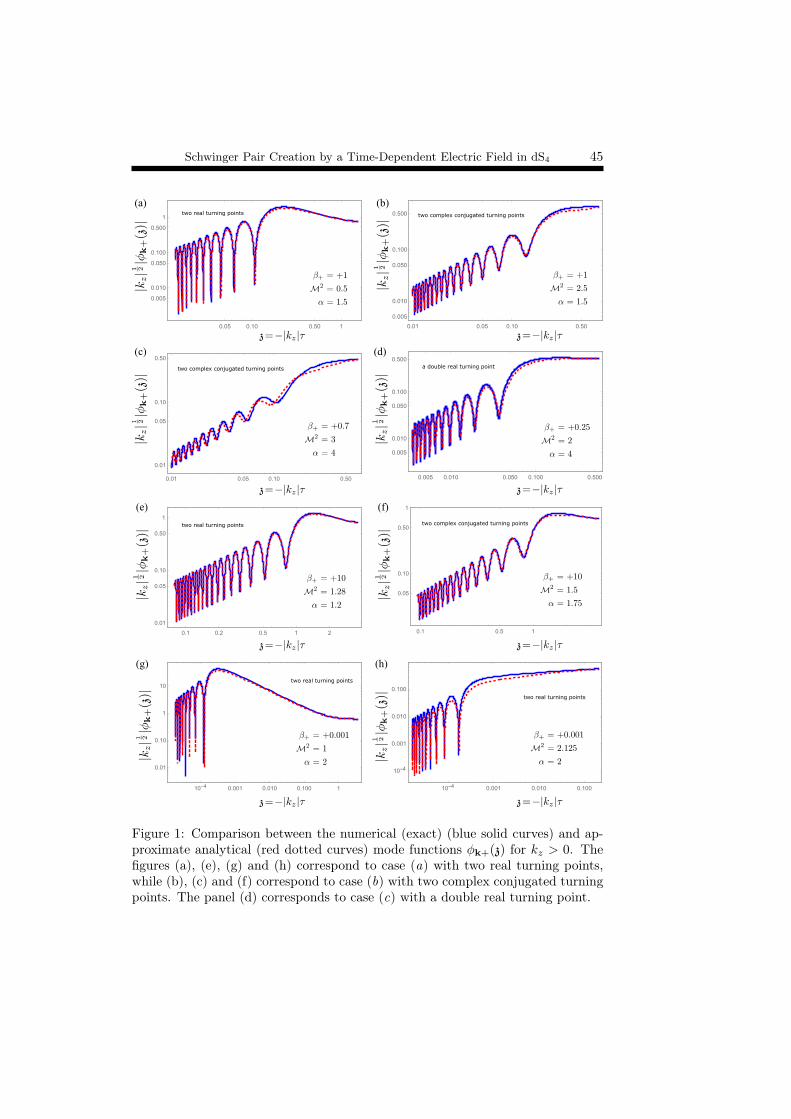
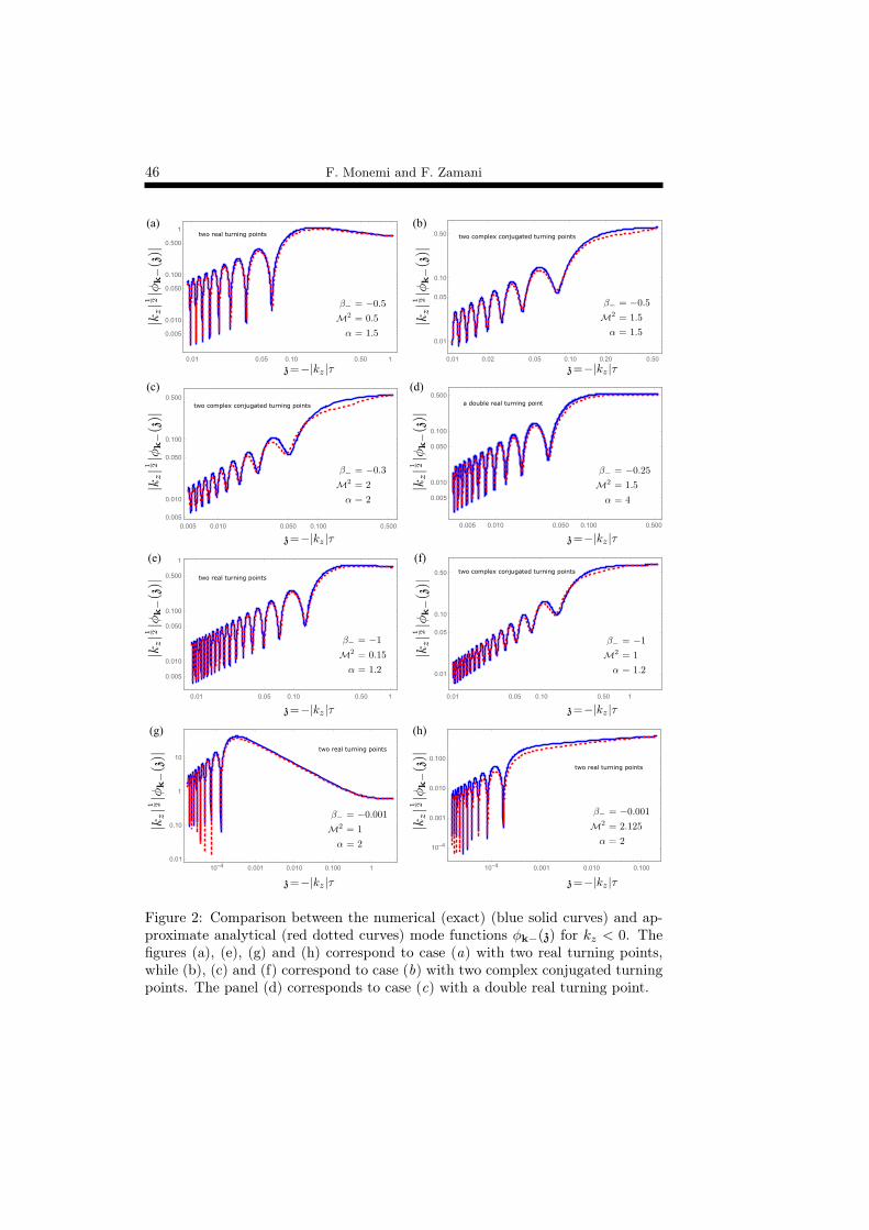
and C2. The analytical approximate solution (19) with C1 and C2 being given byEquation (23) is compared with the numerical solution in Figures 1 (for kz > 0)and 2 (for kz < 0). These figures and many other ones we examined show thatthe exact solution of Equation (9) are well approximated by our first-order ap-proximate analytical solution (19). In the next section we will also observe thatthe pair production probability obtained by these approximate solutions is veryclose to the numerical (exact) value. These observations show that the first-orderapproximation works well and there is no need to extend the solution (19) to highorders.

4. Pair Production ProbabilityHaving obtained the general approximate solutions, let us compute the Schwingerpair production. To do this end, we need to specify the positive- and negative-frequency mode functions that define the so-called in and out vacua.

As pointed out in Section 2, there exist adiabatic in and out vacua correspond-ing, respectively, to the plane wave and WKB solutions in the asymptotic pastand future. Therefore, at early times τ → −∞ (z → +∞), for which we haveλ2g(z) ≃ −α, we choose the normalized positive-frequency solutions ϕ(in,+)

k± (z) tohave the asymptotic form

limz→+∞

ϕ(in,+)k± (z) =

ei√α z√

2|kz|α1/4. (21)

Considering the asymptotic form of the parabolic cylinder functions in the limitz → +∞ (ζ → +∞) given by Equations (34) and (35), the general approximatesolution (19) take the asymptotic form

ϕk±(z) ≃ (−2λg(z))− 1

4 e−π8 λζ2

0

[C1e

iχ(z) + C2e−iχ(z)

], (22)

where, with ϕ2 := phΓ(12 + i

2λζ20

), the function χ(z) is defined by

χ(z) :=

∫ z

z2

√−g(z′) dz′ + π

8− 1

2ϕ2 .


(a) (b)

(c) (d)

(e) (f)

(g) (h)

two real turning points two complex conjugated turning points

a double real turning pointtwo complex conjugated turning points

two real turning points



two complex conjugated turning points

Figure 1: Comparison between the numerical (exact) (blue solid curves) and ap-proximate analytical (red dotted curves) mode functions ϕk+(z) for kz > 0. Thefigures (a), (e), (g) and (h) correspond to case (a) with two real turning points,while (b), (c) and (f) correspond to case (b) with two complex conjugated turningpoints. The panel (d) corresponds to case (c) with a double real turning point.


(a) (b)

(c) (d)

(e) (f)

(g) (h)

two real turning points two complex conjugated turning points

a double real turning pointtwo complex conjugated turning points




two complex conjugated turning points

Figure 2: Comparison between the numerical (exact) (blue solid curves) and ap-proximate analytical (red dotted curves) mode functions ϕk−(z) for kz < 0. Thefigures (a), (e), (g) and (h) correspond to case (a) with two real turning points,while (b), (c) and (f) correspond to case (b) with two complex conjugated turningpoints. The panel (d) corresponds to case (c) with a double real turning point.


Making use of g(z) → −α in the limit z → +∞, one can easily see that the right-hand side of Equation (22) can be matched with the expression (21) if, up to anirrelevant phase factor, we set

C1 = (2λ|kz|2)−1/4 eπ8 λζ2

0 , C2 = 0. (23)

In light of (5) and (19), these integration constants imply that

φ(in,+)k± (x) = a−1(τ)eik·xϕ

(in,+)k± (τ)

= a−1(τ) eik·x|kz|−12 e

π8 λζ2

0

(ζ2 − ζ20−2λg(z)

)14

Dν(√2λζ e−iπ/4) (24)

describes the positive-frequency mode function for the in vacuum. Similarly, thenegative-frequency mode function for the in vacuum can be obtained by C1 = 0and C2 = (2λ|kz|2)−1/4 e

π8 λζ2

0 , i.e., we have

φ(in,−)k± (x) = a−1(τ) e−ik·x|kz|−

12 e

π8 λζ2

0

(ζ2 − ζ20−2λg(z)

)14

D−ν−1(√2λζ eiπ/4). (25)

At late times τ → 0− (z → 0+) the positive-frequency solution of Equation (9)should asymptotically take the form of the WKB solution

ϕ(out,+)k± (z) =

1√2ωk±

e−i∫ωk±dτ ≃ 1√

2|kz|(−g(z))14

exp

[i

∫ z

dz′√

−g(z′)]. (26)

The Liouville-Green approximate solution (18) near the pole z = 0+ matches withthe WKB solution (26) if, up to an irrelevant phase factor, we set c1 = (2λ|kz|)−1/2

and c2 = 0. On the other hand, the negative-frequency solution is simply givenby the choice c1 = 0 and c2 = (2λ|kz|)−1/2. Thus, the positive- and negative-frequency mode functions for the out vacuum can be expressed by

φ(out,+)k± (x) = a−1(τ)eik·xϕ

(out,+)k± (τ)

=a−1(τ) eik·x√2|kz|(−g(z))

14

exp

[i

∫ z

dz′√−g(z′)

], (27)

and φ(out,−)k± (x) = φ

(out,+)k± (x)∗.

Having determined the in and out mode functions (given by Equations (24),(25) and (27)), we can compute the Bogoliubov coefficients. To do this, we use theasymptotic form of φ(in,+)

k± (x) in the infinite future τ → 0− (z → 0+ or ζ → −∞).In view of the asymptotic relation (37), and Equation (27), in this limit we have

limz→0+

ϕ(in,+)k± (z) = lim

ζ→−∞|kz|−

12 e

π8 λζ2

0

(ζ2 − ζ20−2λg(z)

)14

Dν(√2λζ e−iπ/4)

≃ ei(π8 − 1

2ϕ2)√2|kz| (−g(z))

14

[√1 + eπλζ

20 e−iχ(z) − ie

π2 λζ2

0 eiχ(z)]

= ei(π8 − 1

2ϕ2)[√

1 + eπλζ20ϕ

(out,+)k± (z)− ie

π2 λζ2

0ϕ(out,−)k± (z)

],


where in second line we used the notation χ(z) := −∫ z

z1

√−g(z′) dz′. This, in turn,

implies that

φ(in,+)k± (x) ≃

∫d3k′

(2π)3

(αk±,k′φ

(out,+)k′± (x) + βk±,k′φ

(out,−)k′± (x)

),

where the Bogoliubov coefficients αk±,k′ and βk±,k′ are given by

αk±,k′ = (2π)3δ3(k− k′)αk±, αk± =√1 + eπλζ

20 ,

βk±,k′ = (2π)3δ3(k+ k′)βk±, βk± = ieπ2 λζ2

0 .(28)

Here we have ignored the unphysical global phase factor ei(π8 − 1

2ϕ2). These Bogoli-ubov coefficients explicitly satisfy the normalization condition |αk±|2−|βk±|2 = 1.

Now we are in a position to compute the probability of pair production. Thein and out vacua are respectively defined by aoutk|0⟩out = boutk|0⟩out = 0 andaink|0⟩in = bink|0⟩in = 0, for all k, where the late time annihilation operators aoutkand boutk are related to the early time creation and annihilations operators by aBogoliubov transformation [29]

aoutk = αk aink + β∗k b

†in−k , boutk = β∗

−k a†in−k + α−k bink.

In view of this transformation, and Equation (28), for each comoving wave vectork (with positive or negative kz), the number of created pairs in the out vacuum|0⟩out per comoving three-volume is simply given by

out⟨0|a†inkaink|0⟩out(2π)3

∫d3x

=out⟨0|b†in−kbin−k|0⟩out

(2π)3∫d3x

=|βk±|2

(2π)3=eπλζ

20

(2π)3.

Therefore, the nature of the particle creation effect in the background potential (3)can be characterized by the quantity ζ20 . The nature and value of ζ20 , and thereforethe behavior of pair creation strictly depends on the nature of two turning pointsz1 and z2. In the following we treat this issue for three different cases of turningpoints considered in section 3.

Case (a) 0 ≤ M2 < 94 − (

√α∓ 1)|β±| : In this case, to calculate λζ20 , we use

Equations (20) and (15) to write

λζ20 =2

π

∫ z2±

z1±

dz√g(z) =

2√α

π

∫ z2±

z1±

dz

z2

√(z2 − z21±)(z

22± − z2) , (29)

where z1± and z2± are two real turning points given in (16). The integralcan be performed by the change of variable z2 = z22± − (z22± − z21±) sin

2θ. Apart-by-part integration then yields

λζ20 =2

π

√α z2±

(1−

z21±z22±

)∫ π2

0

dθ2 sin2θ − 1√

1−(1− z21±/z

22±

)sin2θ

,


that can be expressed in terms of the complete elliptic integrals of the firstand second kinds K(m) and E(m) [13, 28]. The result is

πλζ20 = 4√α z2±

[(1− m2

2

)K(m)− E(m)

], (30)

where (here 0 < m ≤ 1)

m :=√

1− z21±/z22± =

√2[1 +

(1−

αβ2±

(µ2 + β±)2

)− 12]− 1

2

.

is the modulus of the elliptic functions. The result (30) (more precisely, thepair production probability |βk±|2 = eπλζ

20 ) is compared with the numerical

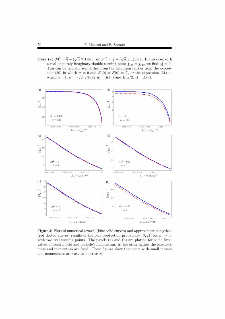
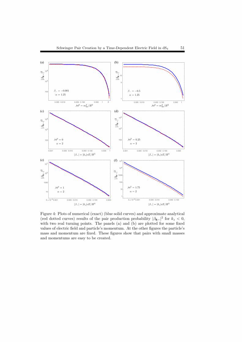
one in Figures 3 (for kz > 0) and 4 (for kz < 0). As can be seen fromthese plots, the more smaller the pair’s mass and momentum are the easierit to be created by the Schwinger mechanism (remember that β± linearlydepends on kz). Also, comparing figures 3 and 4 show that the modes withanti-screening orientations (kz > 0) are hardest to be produced than thosewith screening (kz < 0) orientations.

Case (b) 94 − (

√α∓ 1)|β±| < M2 < 9

4 + (√α± 1)|β±| : In this case, λζ20 = 2π−1∫ z2±

z1±dz√

−g(z) can be expressed by a similar expression as in (29) in whichz1± and z2± stands for the pair of complex conjugate turning points given byEquation (17). Noting that the path of integration lies along the imaginaryaxis, we can use z = ℜ(z1±) + is to perform the integral over s from ℑ(z1±)to ℑ(z2±), where ℑ stands for ‘the imaginary part of ’. The result is

πλζ20 = 4√α ℑ

[z1±

{2(E(n)−E(ψ, n)

)+(n2 − 1)

(K(n)−F (ψ, n)

)+i(n− 1)

√1− (1− 2(n+ 1)−1)

2/4

}], (31)

where F (ψ, n) and E(ψ, n) denote the elliptic integrals of the first and secondkind [13, 28], whose argument ψ and modulus n are defined by

ψ := arcsin(12(1 + n−1)

), n :=

z2±z1±

= eiϑ± .

The result (31) for λζ20 and the corresponding approximate pair productionprobability eπλζ

20 are, respectively, compared with the numerical result of

π−1 ln(|βk±|2

)and |βk±|2 in Figures 5 (for kz > 0) and 6 (for kz < 0). These

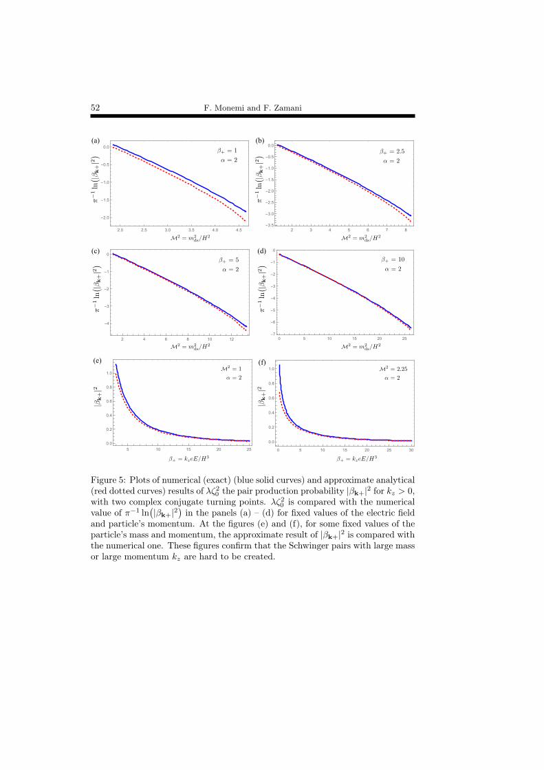
figures indicate that ζ20 is negative for the case of complex turning points andtherefore, in this case, the pair production is exponentially suppressed. Theseplots confirm that (as is physically expected) the more larger the pair’s massand momentum are the harder it to be created. Comparing Figures 5 and6, also, show that the modes with anti-screening orientations (kz > 0) aremore suppressed than those with screening (kz < 0) orientations.


Case (c) M2 = 94 − (

√α∓ 1)|β±| or M2 = 9

4 + (√α± 1)|β±| : In this case, with

a real or purely imaginary double turning point z1± = z2±, we find ζ20 = 0.This can be trivially seen either from the definition (20) or from the expres-sion (30) in which m = 0 and K(0) = E(0) = π

2 , or the expression (31) inwhich n = 1, ψ = π/2, F (π/2, n) = K(n) and E(π/2, n) = E(n).

(a) (b)

(c) (d)

(e) (f)

2

3

Figure 3: Plots of numerical (exact) (blue solid curves) and approximate analytical(red dotted curves) results of the pair production probability |βk+|2 for kz > 0,with two real turning points. The panels (a) and (b) are plotted for some fixedvalues of electric field and particle’s momentum. At the other figures the particle’smass and momentum are fixed. These figures show that pairs with small massesand momentums are easy to be created.


(a) (b)

(c) (d)

(e) (f)

2

Figure 4: Plots of numerical (exact) (blue solid curves) and approximate analytical(red dotted curves) results of the pair production probability |βk−|2 for kz < 0,with two real turning points. The panels (a) and (b) are plotted for some fixedvalues of electric field and particle’s momentum. At the other figures the particle’smass and momentum are fixed. These figures show that pairs with small massesand momentums are easy to be created.


(a) (b)

(c) (d)

(e) (f)

Figure 5: Plots of numerical (exact) (blue solid curves) and approximate analytical(red dotted curves) results of λζ20 the pair production probability |βk+|2 for kz > 0,with two complex conjugate turning points. λζ20 is compared with the numericalvalue of π−1 ln

(|βk+|2

)in the panels (a) – (d) for fixed values of the electric field

and particle’s momentum. At the figures (e) and (f), for some fixed values of theparticle’s mass and momentum, the approximate result of |βk+|2 is compared withthe numerical one. These figures confirm that the Schwinger pairs with large massor large momentum kz are hard to be created.


(a) (b)

(c) (d)

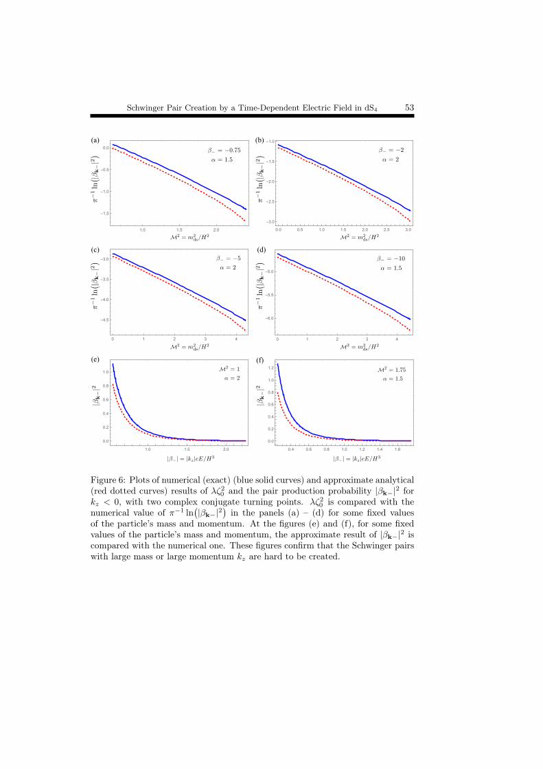
(e) (f)

Figure 6: Plots of numerical (exact) (blue solid curves) and approximate analytical(red dotted curves) results of λζ20 and the pair production probability |βk−|2 forkz < 0, with two complex conjugate turning points. λζ20 is compared with thenumerical value of π−1 ln

(|βk−|2

)in the panels (a) – (d) for some fixed values

of the particle’s mass and momentum. At the figures (e) and (f), for some fixedvalues of the particle’s mass and momentum, the approximate result of |βk−|2 iscompared with the numerical one. These figures confirm that the Schwinger pairswith large mass or large momentum kz are hard to be created.


The numerical value for |βk±|2 can be obtained from the numerical solutionsof Equation (9). For this purpose, we first notice that when z approaches zero,one can choose the positive- and negative-frequency out-modes as (compare withthe WKB solution (26))

ϕ(out,+)k± (z) =

z√|kz| |β±|

exp[− i

|β±|2z

], ϕ

(out,−)k± (z) = ϕ

(out,+)k± (z)∗,

which solve the asymptotic equation d2ϕk±/dz2 +

(β2/(4z2)

)ϕk± = 0 and are

normalized with the inner product(ϕ1(z), ϕ2(z)

)= i

[ϕ1(z)

∗ ϕ′2(z) − ϕ′1(z)∗ ϕ2(z)

],

where ϕ′ = ∂τϕ = −|kz|∂zϕ. Also, we take the expression (21) as the initial condi-tion to obtain the numerical solution ϕk±(z) and its derivative. Then, according tothe expansion ϕk±(z) = αk± ϕ

(out,+)k± (z) + βk± ϕ

(out,−)k± (z), we can use a very small

value for z (z → 0) to compute |βk±|2 =∣∣(ϕk±(z), ϕ(out,−)

k± (z))∣∣2. This numerical

result is compared with the analytical value |βk±|2 = eπλζ20 in Figures 3 and 5 for

kz > 0 and Figures 4 and 6 for kz < 0.

3.3 Weak Electric Field Limit

For the weak electric field eE ≪ H2 (E ≪ 1), the parameter |β±| is small, andhence the modulus m of the elliptic functions is close to one. This means thatthe complementary modulus m′ :=

√1−m2 is small and one can use the series

expansions [13]

K(m) = ln4

m′ +1

4

(ln

4

m′ − 1)m′2 +

9

64

(ln

4

m′ −7

6

)m′4 + · · · ,

E(m) = 1 +1

2

(ln

4

m′ −1

2

)m′2 +

3

16

(ln

4

m′ −13

12

)m′4 + · · · ,

for the elliptic functions in Equation (30) to find the approximate value of ζ20 inthe powers of β± (or E). The result is

πλζ20 ≃ 2√µ2

{− 2 +

(1± |β±|

2µ2

)ln( 8µ2

|β±|√α

)+O(β2

±)}

=

√9

4−m2

ds

H2

{6 ln 2− 4 + 2 ln

(94− m2

ds

H2

)− ln

(1 +

k2⊥k2z

)− 2 ln

(eE|kz|H3

)±(eE|kz|

H3

)(94− m2

ds

H2

)−1

ln

(8(94− m2

ds

H2

)(1 +

k2⊥k2z

)−1/2)

∓(94− m2

ds

H2

)−1(eE|kz|H3

)ln(eE|kz|

H3

)+O(E2)

}, (32)


where we recall that k2⊥ = k2x + k2y. Thus, in view of the result (32), in the weakelectric field limit, pair production probability |βk±|2 = eπλζ

20 behaves as

|βk±|2 ∝(

H3

eE|kz|

)2

√94−

m2ds

H2

,

which diverges as eE|kz|/H3 → 0 (see Figures 3-c to 3-f and 4-c to 4-f).Though we can not compute the renormalized induced electric current (because

we have not at hand any everywhere-defined expression for the mode functionsϕk±(z)), instead, following [8], in the weak electric field limit, we can find thesemiclassical current J as

J ∝(|βk−|2 − |βk+|2

)≈ C

(eE|kz|H3

)1−2

√94−

m2ds

H2[1− ln

(eE|kz|H3

)]+O(Eδ),

where δ = 2− 2√9/4−m2

ds/H2 and

C := −2(µ2

)−1/2e−4

√µ2(64(µ2)2

α

)√µ2

ln(8µ2

√α

).

Similar to the case studied in [11], there exists a critical mass mcr =√2H, below

which the electric current J exhibits the so-called infrared hyperconductivity, whichhas been initially observed in [8] (only for m = 0 in the presence of a uniformelectric field background in (1+1)-dimensional de Sitter space). Indeed, for mds ∈(0,

√2H), when E goes to zero, the electric current J diverges as 1/E 2∆, where

∆ :=√

9/4−m2ds/H

2 − 12 ∈ (0, 1). In particular, when mds = 0, J is inversely

proportional to E2. This divergence behavior is two times faster than the casesconsidered in [8, 11]. In addition, unlike the case of [11], here for mds = mcr =√2H, J exhibits also a logarithmic divergence in the limit eE|kz|/H3 → 0.

5. ConclusionIn this work, we have investigated the Schwinger pair creation by a time-dependentelectric field in (1+3)-dimensional de Sitter spacetime. Specifically, in dS4, wehave considered a charged scalar field, as a test field, coupled to a time-dependentbackground electric field (3) which has a time-dependent energy density in theexpanding universe. We have seen that, while the field equation of motion doesnot admit an exact analytical solution, it can be solved by means of Olver’s uniformasymptotic approximation method. We showed that the equation of motion, ingeneral, has two turning points, whose natures (single, double, real or complex)depend on the value of the electric field E, the particle’s massm, and wave vector k.Using the first-order approximate solutions (the mode functions for the canonical


quantization) the Bogoliubov coefficients and consequently the probability for thepair production were computed both analytically and numerically, which strictlydepends on the natures of the turning points. More precisely, we found thatthe pair creation process is enhanced when the two turning points are real andsingle, and suppressed when they are complex conjugate. Furthermore, when theparticle’s mass and momentum are small, two turning points are real, and themore smaller are the easier to create particles by the Schwinger mechanism. Formassive particles or large momentums, both turning points are complex, and theSchwinger pair creation is exponentially suppressed. In addition, for both cases ofreal and complex turning points, we explored that the modes with anti-screeningorientation (kz > 0) are different from those with screening orientation (kz < 0)in pair production process. Indeed, light (massive) particles with anti-screeningorientations are hardest to be produced (are more suppressed) than those withscreening orientations.

For small particle’s mass and momentum, in the weak electric field limit, wealso computed analytically the pair production probability and the semi-classicalelectric current induced by the created Schwinger pairs. Remarkably, we foundthat the pair creation probability |βk±|2 and hence the semi-classical current J arestrongly enhanced as the electric field diminishes. Indeed, as E → 0, pair creationprobability and the semi-classical current diverge, respectively, as 1/E2∆+1 and1/E2∆ (1− lnE), where ∆ :=

√9/4−m2

ds/H2 − 1

2 ∈ (0, 1). This means that,similar to the case studied in [11], there exists a critical mass mcr =

√2H, below

which the electric current J exhibits the so-called infrared hyperconductivity thatstems from the infrared behavior of light fields in de Sitter spacetime. For aconstant electric field background, this negative conductivity shows itself in theregularized electric current [3, 8, 21]. But, it is recently argued in [1] that thisspurious is a byproduct of nonlinear corrections to the Maxwell action and thelogarithmic running of the coupling constant.

Appendix: Weber’s Equation, Parabolic Cylinder Functionsand their Asymptotic ExpansionIn this appendix, we present the detailed derivation of the general solution (19)of equation d2U/dζ2 =

[λ2(ζ20 − ζ2)

]U , and elaborate on their asymptotic ex-

pansions. It can be easily seen that in terms of the variable ζ :=√λ (1 − i)ζ =√

2λ ζ e−iπ/4, this equation can be cast into the form of the so-called Weber’sequation [40]

d2U

dζ2+

[1

2+ ν − 1

4ζ2]U = 0, (33)

where ν := − 12 − i

2 λ ζ20 . The parabolic cylinder functions Dν(ζ) satisfy the dif-

ferential equation (33). Because Equation (33) is unaltered if we simultaneouslyapply the changes ζ → iζ and ν → −ν − 1, we can choose Dν(

√2λ ζ e−iπ/4) and

D−ν−1(√2λ ζ eiπ/4) as two linearly independent solutions of equation d2U/dζ2 =


[λ2(ζ20 − ζ2)

]U . Thus, the general asymptotic solution near two turning points z1

and z2 can be written as in Equation (19).Next, in view of the relation Dν(ζ) = U(− 1

2 − ν, ζ) and the asymptotic expan-sions for Weber parabolic cylinder function U(a, ζ) that is given in [25], we observethat the asymptotic expansion of Dν(ζ) of large order ζ20 in the limit ζ → +∞ canbe expressed as

D− 12−

i2λζ

20(√2λ ζ e−iπ/4) ≃ eiλ ζ2

0 ξ(ζ)

(ζ2 − ζ20 )1/4

h(√λζ0 e

−iπ/4), (34)

D− 12+

i2λζ

20(√2λ ζ eiπ/4) ≃ e−iλ ζ2

0 ξ(ζ)

(ζ2 − ζ20 )1/4

h(√λζ0 e

iπ/4), (35)

where ξ(ζ) is defined by

ζ20 ξ(ζ) :=

∫ ζ

ζ0

dζ ′√ζ ′2 − ζ20 =

1

2ζ√ζ2 − ζ20 − 1

2ζ20 arccosh(ζ/ζ0),

h(√λζ0 e

−iπ4 ) is approximately given by

h(√λζ0 e

−iπ/4) ≃ (2λ)−14 e−π

λζ208 ei(

π8 − 1

2ϕ2),

h(√λζ0e

iπ4 )=(h(

√λζ0e

−iπ4 ))∗, and ϕ2 :=phΓ

(12+

i2λζ

20

)is the phase of Γ

(12+

i2λζ

20

).

To find the asymptotic expansion of Dν(√2λ ζ e−iπ/4) of large order ζ20 in the

limit ζ → −∞, we use the connection formula [40, 28]

Dν(−√2λζe−iπ

4 ) = eiπνDν(√2λζe−iπ

4 ) + i eiπν/2√2π

Γ(−ν)D−ν−1(

√2λζei

π4 ). (36)

Substituting Equations (34) and (35) in Equation (36) and making use of theidentities ie−iπ/4h(

√λζ0e

iπ4 ) = h(

√λζ0e

−iπ4 ) and

Γ(1

2+i

2λζ20 ) =

√π(cosh(

πλζ202

))−1/2 eiϕ2 ,

we find that, for large order ζ20 , the asymptotic form of Dν(√2λ ζ e−iπ/4) in the

limit ζ → −∞ can be written as

D− 12−

i2λζ

20(√2λ ζ e−iπ/4) ≃ h(

√λζ0 e

−iπ/4)

(ζ2 − ζ20 )1/4

[√1 + eπλζ

20 e−iλ ζ2

0 ξ′(ζ)

−ieπλζ20/2 eiλ ζ2

0 ξ′(ζ)], (37)

where ξ′(ζ) is defined by

ζ20 ξ′(ζ) :=

∫ ζ

−ζ0

dζ ′√ζ ′2 − ζ20 = −1

2ζ√ζ2 − ζ20 − 1

2ζ20 arccosh(−ζ/ζ0).

Conflicts of Interest. The authors declare that there are no conflicts of interestregarding the publication of this article.


References[1] M. Banyeres, G. Domènech and J. Garriga, Vacuum birefringence and the

Schwinger effect in (3+1) de Sitter, J. Cosmol. Astropart. Phys. 10 (2018)023.

[2] D. Baumann and L. McAllister, Inflation and String Theory, Cambridge Uni-versity Press, Cambridge, UK, 2015.

[3] E. Bavarsad, C. Stahl and S. -S. Xue, Scalar current of created pairs bySchwinger mechanism in de Sitter spacetime, Phys. Rev. D 94 (2016) 104011.

[4] R. G. Cai and S. P. Kim, One-loop effective action and Schwinger effect in(anti-) de Sitter space, J. High Energy Phys. 09 (2014) 072.

[5] S. M. Carroll, The Cosmological Constant, Living Rev. Relativity 3 (2001)1− 56.

[6] A. Di Piazza, C. Müller, K. Z. Hatsagortsyan and C. H. Keitel, Extremelyhigh-intensity laser interactions with fundamental quantum systems, Rev.Mod. Phys. 84 (2012) 1117− 1228.

[7] R. Emami, H. Firouzjahi, S. M. Sadegh Movahed and M. Zarei, Anisotropicinflation from charged scalar fields, J. Cosmol. Astropart. Phys. 02 (2011)005.

[8] M. B. Fröb, J. Garriga, S. Kanno, M. Sasaki, J. Soda, T. Tanaka and A.Vilenkin, Schwinger effect in de Sitter space, J. Cosmol. Astropart. Phys. 04(2014) 009.

[9] J. Garriga, Pair production by an electric field in (1+1)-dimensional de Sitterspace, Phys. Rev. D 49 (1994) 6343− 6346.

[10] F. Gelis and N. Tanji, Schwinger mechanism revisited, Prog. Part. Nucl. Phys.87 (2016) 1− 49.

[11] J.-J. Geng, B.-F. Li, J. Soda, A. Wang, Q. Wu and T. Zhu, Schwinger pairproduction by electric field coupled to inflaton, J. Cosmol. Astropart. Phys.02 (2018) 018.

[12] M. Giovannini, Spectator electric fields, de Sitter spacetime, and theSchwinger effect, Phys. Rev. D 97 (2018) 061301(R).

[13] I. S. Gradshteyn and I. M. Ryzhik, Table of Integrals, Series and Products,7th ed., Academic Press, Amsterdam, 2007.

[14] S. Haouat and R. Chekireb, Effect of electromagnetic fields on the creationof scalar particles in a flat Robertson-Walker spacetime, Eur. Phys. J. C 72(2012) 2034.


[15] S. Haouat and R. Chekireb, Schwinger effect in a Robertson-Walker space-time, Int. J. Theor. Phys. 51 (2012) 1704− 1714.

[16] T. Hayashinaka, T. Fujita and J. Yokoyama, Fermionic Schwinger effect andinduced current in de Sitter space, J. Cosmol. Astropart. Phys. 07 (2016) 010.

[17] T. Hayashinaka and J. Yokoyama, Point splitting renormalization ofSchwinger induced current in de Sitter spacetime, J. Cosmol. Astropart. Phys.07 (2016) 012.

[18] W. Heisenberg and H. Euler, Consequences of Dirac’s theory of positrons, Z.Phys. 98 (1936) 714− 732.

[19] S. P. Kim and D. N. Page, Schwinger pair production in dS2 and AdS2, Phys.Rev. D 78 (2008) 103517.

[20] H. Kitamoto, Schwinger effect in inflation-driven electric field, Phys. Rev. D98 (2018) 103512.

[21] T. Kobayeshi and N. Afshordi, Schwinger effect in 4D de Sitter space andconstraints on magnetogenesis in the early Universe, J. High Energy Phys. 10(2014) 166.

[22] J. Martin, Inflationary Perturbations: The Cosmological Schwinger Effect,in: Inflationary Cosmology, Lecture Notes in Physics, vol. 738, 193 − 241,Springer-Verlag, Berlin, 2007.

[23] S. Moradi, Particle production in cosmological spacetimes with electromag-netic fields, Mod. Phys. Lett. A 24 (2009) 1129− 1136.

[24] A. H. Nayfeh, Perturbation Methods, Wiley, New York, 1973.

[25] F. W. J. Olver, Uniform asymptotic expansions for Weber parabolic cylinderfunctions of large orders, J. Res. Nat. Bur. Standards, Sect. B: Math. andMath. Phys. 63B (1959) 131− 169.

[26] F. W. J. Olver, Second-order linear differential equations with two turningpoints, Philos. Trans. Roy. Soc. A 278 (1975) 137− 174.

[27] F. W. J. Olver, Asymptotics and Special Functions, AKP Classics, Wellesley,MA, 1997.

[28] F. W. J. Olver, D. W. Lozier, R. F. Boisvert and C. W. Clark, NIST Hand-book of Mathematical Functions, Cambridge University Press, Cambridge,UK, 2010.

[29] L. Parker and D. Toms, Quantum Field Theory in Curved Space: QuantizedFields and Gravity, Cambridge University Press, Cambridge, UK, 2009.


[30] R. Ruffini, G. Vereshchagin and S. S. Xue, Electron-positron pairs in physicsand astrophysics: from heavy nuclei to black holes, Phys. Rept. 487 (2010)1− 140.

[31] F. Sauter, Über das verhalten eines electrons im homogenen electrischen feldnach der relativistischen theorie Diracs, Z. Phys. 69 (1931) 742− 764.

[32] J. S. Schwinger, On gauge invariance and vacuum polarization, Phys. Rev. 82(1951) 664− 679.

[33] S. Shakeri, M. A. Gorji and H. Firouzjahi, Schwinger mechanism during in-flation, Phys. Rev. D 99 (2019) 103525.

[34] R. Sharma and S. Singh, Multifaceted Schwinger effect in de Sitter space,Phys. Rev. D 96 (2017) 025010.

[35] K. Sogut, A. Havare, On the scalar particle creation by electromagnetic fieldsin Robertson-Walker spacetime, Nucl. Phys. B 901 (2015) 76− 84.

[36] C. Stahl, E. Strobel and S.-S. Xue, Fermionic current and Schwinger effect inde Sitter spacetime, Phys. Rev. D 93 (2016) 025004.

[37] V. M. Villalba, Creation of spin- 12 particles by an electric field in de Sitterspace, Phys. Rev. D 52 (1995) 3742− 3745.

[38] V. M. Villalba and W. Greiner, Creation of scalar and Dirac particles inthe presence of a time varying electric field in an anisotropic Bianchi type Iuniverse, Phys. Rev. D 65 (2001) 025007.

[39] M.-a. Watanabe, S. Kanno and J. Soda, Inflationary universe with anisotropichair, Phys. Rev. Lett. 102 (2009) 191302.

[40] E. T. Whittaker and G. N. Watson, A Course of Modern Analysis, 2nd ed.,Cambridge University Press, Cambridge, UK, 1915.

[41] T. Zhu, A. Wang, G. Cleaver, K. Kirsten and Q. Sheng, Constructing ana-lytical solutions of linear perturbations of inflation with modified dispersionrelations, Int. J. Modern Phys. A 29 (2014) 1450142.

[42] T. Zhu, A. Wang, G. Cleaver, K. Kirsten and Q. Sheng, Inflationary cosmol-ogy with nonlinear dispersion relations, Phys. Rev. D 89 (2014) 043507.

[43] T. Zhu, A. Wang, G. Cleaver, K. Kirsten and Q. Sheng, Gravitational quan-tum effects on power spectra and spectral indices with higher-order correc-tions, Phys. Rev. D 90 (2014) 063503.

[44] T. Zhu, A. Wang, K. Kirsten, G. Cleaver and Q. Sheng, High-order primordialperturbations with quantum gravitational effects, Phys. Rev. D 93 (2016)123525.


Fatemeh MonemiDepartment of Physics,University of Kashan,Kashan, I. R. Irane-mail: [email protected]

Farhad ZamaniDepartment of Physics,University of Kashan,Kashan, I. R. Irane-mail: [email protected]

Schwinger Pair Creation by a Time-Dependent Electric Field ...

Documents

Transcript of Schwinger Pair Creation by a Time-Dependent Electric Field ...