Cosmology & CMB

Set2: Linear Perturbation Theory

Davide Maino

Covariant Perturbation Theory

• Covariant= takes sameform in all coordinate systems

• Invariant= takes the samevaluein all coordinate systems

• Fundamental equations:Einstein equations, (covariant)conservationof stress-energy tensor:

Gµν = 8πGTµν

∇µTµν = 0

• how manydegrees of freedom: 10 for a symmetric 4× 4 tensor

• perturbations aresmall: look at CMB where fluctuations are∼ 10−5

Metric Tensor

• Expand metric tensor around thegeneral FRW metric

g00 = −a2, gij = a2γij .

• Add in general perturbation (Bardeen 1980)

g00 = −a−2(1− 2A)

g0i = −a−2Bi

gij = a−2(γij − 2HLγij − 2HijT)

• (1) A ≡ a scalarpotential; (3) Bi a vectorshift, (1) HL aperturbation in the spatialcurvature; (5) Hij

T a tracelessdistortionto spatial metric =(10)

Matter Tensor

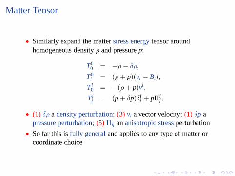
• Similarly expand the matterstress energytensor aroundhomogeneous densityρ and pressurep:

T00 = −ρ − δρ,

T0i = (ρ + p)(vi − Bi),

T i0 = −(ρ + p)vi,

T ij = (p + δp)δi

j + pΠij,

• (1) δρ adensity perturbation; (3) vi a vector velocity;(1) δp apressure perturbation; (5) Πij ananisotropic stressperturbation

• So far this isfully generaland applies to any type of matter orcoordinate choice

Gauge

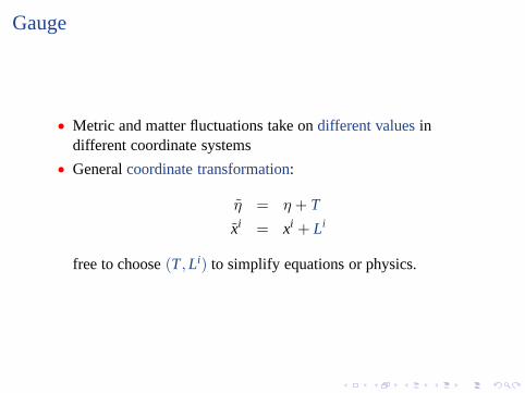
• Metric and matter fluctuations take ondifferent valuesindifferent coordinate systems

• Generalcoordinate transformation:

η = η + T

xi = xi + Li

free to choose(T, Li) to simplify equations or physics.

Newtonian Gauge

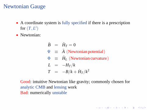
• A coordinate system isfully specifiedif there is a prescriptionfor (T, Li)

• Newtonian:

B = HT = 0

Ψ ≡ A (Newtonian potential)

Φ ≡ HL (Newtonian curvature)

L = −HT/k

T = −B/k + HT/k2

Good: intuitive Newtonian like gravity; commonly chosen foranalytic CMBandlensingworkBad: numericallyunstable

Newtonian Gauge

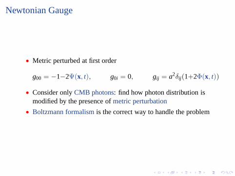
• Metric perturbed at first order

g00 = −1−2Ψ(x, t), g0i = 0, gij = a2δij(1+2Φ(x, t))

• Consider onlyCMB photons: find how photon distribution ismodified by the presence ofmetric perturbation

• Boltzmann formalismis the correct way to handle the problem

Boltzmann Equation

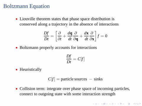
• Liouville theorem states that phase space distribution isconserved along a trajectory in the absence of interactions

DfDt

=

[

∂

∂t+

dqdt

∂

∂q+

dxdt

∂

∂x

]

f = 0

• Boltzmann properly accounts for interactions

DfDt

= C[f ]

• Heuristically

C[f ] = particle sources− sinks

• Collision term: integrate over phase space of incoming particles,connect to outgoing state with some interaction strength

LHS of Boltzmann Equation

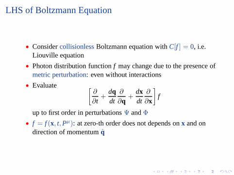
• ConsidercollisionlessBoltzmann equation withC[f ] = 0, i.e.Liouville equation

• Photon distribution functionf may change due to the presence ofmetric perturbation: even without interactions

• Evaluate[

∂

∂t+

dqdt

∂

∂q+

dxdt

∂

∂x

]

f

up to first order in perturbationsΨ andΦ

• f = f (x, t, Pµ): at zero-th order does not depends onx and ondirection of momentumq

LHS of Boltzmann Equation

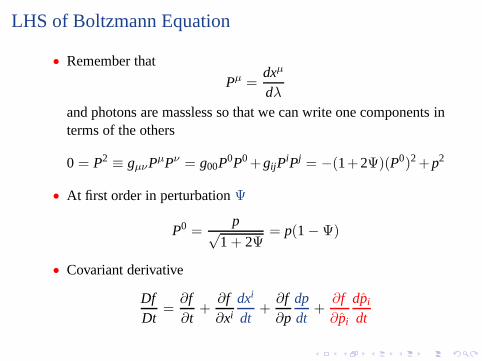
• Remember that

Pµ =dxµ

dλ

and photons are massless so that we can write one components interms of the others

0 = P2 ≡ gµνPµPν = g00P0P0+gijPiPj = −(1+2Ψ)(P0)2+p2

• At first order in perturbationΨ

P0 =p√

1 + 2Ψ= p(1− Ψ)

• Covariant derivative

DfDt

=∂f∂t

+∂f∂xi

dxi

dt+

∂f∂p

dpdt

+∂f∂pi

dpi

dt

dxi

dt

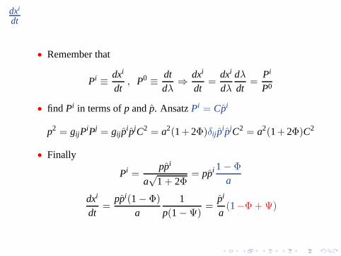
• Remember that

Pi ≡ dxi

dt, P0 ≡ dt

dλ⇒ dxi

dt=

dxi

dλ

dλ

dt=

Pi

P0

• find Pi in terms ofp andp. AnsatzPi = Cpi

p2 = gijPiPj = gijp

ipjC2 = a2(1+ 2Φ)δijpipjC2 = a2(1+ 2Φ)C2

• Finally

Pi =ppi

a√

1 + 2Φ= ppi 1− Φ

a

dxi

dt=

ppi(1− Φ)

a1

p(1− Ψ)=

pi

a(1−Φ + Ψ)

dpdt

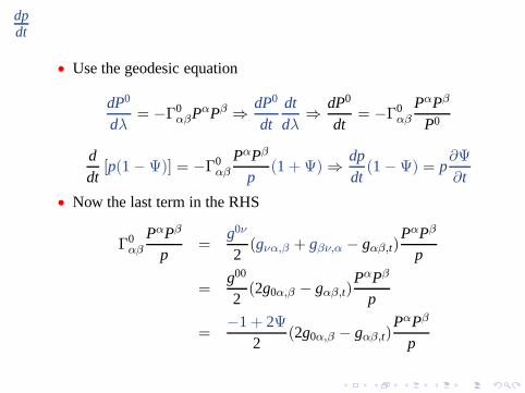
• Use the geodesic equation

dP0

dλ= −Γ0

αβPαPβ ⇒ dP0

dtdtdλ

⇒ dP0

dt= −Γ0

αβ

PαPβ

P0

ddt

[p(1− Ψ)] = −Γ0αβ

PαPβ

p(1 + Ψ) ⇒ dp

dt(1− Ψ) = p

∂Ψ

∂t

• Now the last term in the RHS

Γ0αβ

PαPβ

p=

g0ν

2(gνα,β + gβν,α − gαβ,t)

PαPβ

p

=g00

2(2g0α,β − gαβ,t)

PαPβ

p

=−1 + 2Ψ

2(2g0α,β − gαβ,t)

PαPβ

p

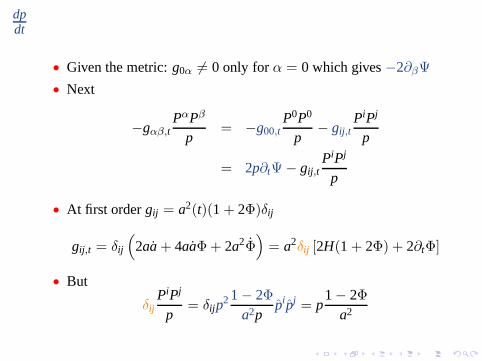
dpdt

• Given the metric:g0α 6= 0 only forα = 0 which gives−2∂βΨ

• Next

−gαβ,tPαPβ

p= −g00,t

P0P0

p− gij,t

PiPj

p

= 2p∂tΨ − gij,tPiPj

p

• At first ordergij = a2(t)(1 + 2Φ)δij

gij,t = δij

(

2aa + 4aaΦ + 2a2Φ)

= a2δij [2H(1 + 2Φ) + 2∂tΦ]

• But

δijPiPj

p= δijp

21− 2Φ

a2ppipj = p

1− 2Φ

a2

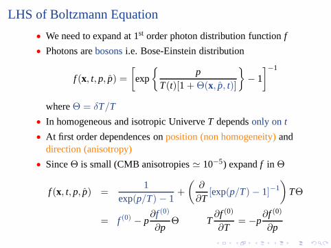
LHS of Boltzmann Equation

• We need to expand at 1st order photon distribution functionf

• Photons arebosonsi.e. Bose-Einstein distribution

f (x, t, p, p) =

[

exp

pT(t)[1 + Θ(x, p, t)]

− 1

]

−1

whereΘ = δT/T

• In homogeneous and isotropic UniverveT dependsonly on t

• At first order dependences onposition (non homogeneity)anddirection (anisotropy)

• SinceΘ is small (CMB anisotropies≃ 10−5) expandf in Θ

f (x, t, p, p) =1

exp(p/T) − 1+

(

∂

∂T[exp(p/T) − 1]−1

)

TΘ

= f (0) − p∂f (0)

∂pΘ T

∂f (0)

∂T= −p

∂f (0)

∂p

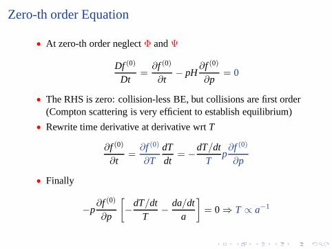
Zero-th order Equation

• At zero-th order neglectΦ andΨ

Df (0)

Dt=

∂f (0)

∂t− pH

∂f (0)

∂p= 0

• The RHS is zero: collision-less BE, but collisions are first order(Compton scattering is very efficient to establish equilibrium)

• Rewrite time derivative at derivative wrtT

∂f (0)

∂t=

∂f (0)

∂TdTdt

= −dT/dtT

p∂f (0)

∂p

• Finally

−p∂f (0)

∂p

[

−dT/dtT

− da/dta

]

= 0 ⇒ T ∝ a−1

First order Equation

• Eliminating the zero-th order equation from the LHS we getretaining only 1st order terms

Df (1)

Dt= −p

∂f (0)

∂p

[

∂Θ

∂t+

pi

a∂Θ

∂xi +∂Φ

∂t+

pi

a∂Ψ

∂xi

]

• free-streamingi.e. anisotropies down to small scales

• gravity effect on photon distribution

RHS of Boltzmann Equation

• Form:

C[f ] =

∫

d(phase space)[energy− momentum conservation]

× |M|2[emission− absorption]

• Matrix elementM contains physics of interaction (Comptonscattering)

• (Lorentz invariant) phase space element

∫

d(phase space) = Πigi

(2π)3

∫

d3qi

2Ei

• Conservation:(2π)4δ(4)(q1 + q2 + . . . )

RHS of Boltzmann Equation

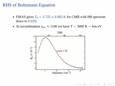
• FIRAS givesT0 = 2.725± 0.002 K for CMB with BB spectrumdown to0.02%

• At recombinationzrec ≈ 1100 we haveT ∼ 3000 K∼ few eV

Compton Scattering

• Photons and electrons interact via Compton scatteringγ′ + e−′ ↔ γ + e− and Coulomb interaction link photons tobaryons

C[f ] =1

2E(q)

∫

DqeDq′eDq′(2π)4δ(4)(q + qe − q′ − q′e)

[fe(q′

e)f (q′) − fe(qe)f (q)]|M|2

• Small energy transfer implies:non-relativisticComptonscattering;q ≃ q′ andqe ≫ q, q′

• Breakδ(4) into energy and momentum conservation

• Expand at first order around electron energy change

• Scattering Matrix|M|2 = 8πσT m2e: no angular dependence

|M|2

• |M|2 = 8πσT m2e is wrong for two reasons

• There is an angular dependence|M|2 ∝ (1 + cos[q · q′]): smalldifference (down to 1% level)

• |M|2 has also a polarisation dependence∝ |ǫ · ǫ′| whereǫ andǫ′

are polarization of incoming and outgoing photons

• When Compton is efficient this dependence is removed (youaverage on all possible directions uniformly)

• Nearrecombinationthis is no more true→ quadrupoleanisotropyis produced leaving a netlinear polarizationin theCMB

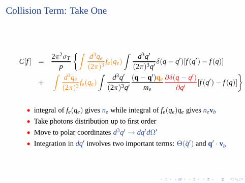
Collision Term: Take One

C[f ] =2π2σT

p

∫

d3qe

(2π)3 fe(qe)

∫

d3q′

(2π)3q′δ(q − q′)[f (q′) − f (q)]

+

∫

d3qe

(2π)3 fe(qe)

∫

d3q′

(2π)3q′(q − q′)qe

me

∂δ(q − q′)∂q′

[f (q′) − f (q)]

• integral offe(qe) givesne while integral offe(qe)qe givesnevb

• Take photons distribution up to first order

• Move to polar coordinatesd3q′ → dq′dΩ′

• Integration indq′ involves two important terms:Θ(q′) andq′ · vb

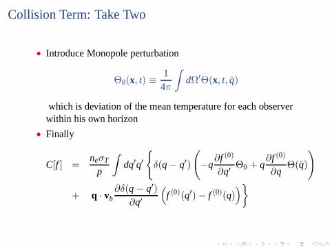
Collision Term: Take Two

• Introduce Monopole perturbation

Θ0(x, t) ≡ 14π

∫

dΩ′Θ(x, t, q)

which is deviation of the mean temperature for each observerwithin his own horizon

• Finally

C[f ] =neσT

p

∫

dq′q′

δ(q − q′)

(

−q∂f (0)

∂q′Θ0 + q

∂f (0)

∂qΘ(q)

)

+ q · vb∂δ(q − q′)

∂q′

(

f (0)(q′) − f (0)(q))

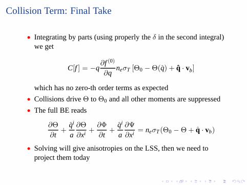
Collision Term: Final Take

• Integrating by parts (using properly theδ in the second integral)we get

C[f ] = −q∂f (0)

∂qneσT [Θ0 − Θ(q) + q · vb]

which has no zero-th order terms as expected

• Collisions driveΘ to Θ0 and all other moments are suppressed

• The full BE reads

∂Θ

∂t+

qi

a∂Θ

∂xi +∂Φ

∂t+

qi

a∂Ψ

∂xi = neσT(Θ0 − Θ + q · vb)

• Solving will give anisotropies on the LSS, then we need toproject them today