to (to ) Time Dependent CP-8.5-.25ex analysis - B2TIP...

B0 → η′(→ ηπ+π−)K0S Time Dependent ��CP analysis

B2TIP practice talk(plus other minor stuff not for B2TIP)

Stefano [email protected]

INFN Padova

WG3 meeting,virtual, 18 May 2016

S.Lacaprara (INFN Padova) B0 → η

′K

0S WG3 18/05/2016 1 / 23

mailto:[email protected]

Introduction and motivations

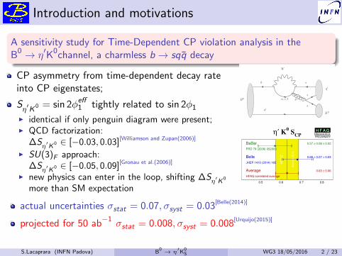
A sensitivity study for Time-Dependent CP violation analysis in theB0 → η′K0channel, a charmless b → sqq decay

CP asymmetry from time-dependent decay rateinto CP eigenstates;

Sη′K

0 = sin 2φeff1 tightly related to sin 2φ1

I identical if only penguin diagram were present;I QCD factorization:

∆Sη′K 0 ∈ [−0.03, 0.03][Williamson and Zupan(2006)]

I SU(3)F approach:∆Sη′K 0 ∈ [−0.05, 0.09][Gronau et al.(2006)]

I new physics can enter in the loop, shifting ∆Sη′K 0

more than SM expectation

B0

η′

K0

b

d

s

s

s

g

W

u, c, t

η′ K0 S

CP

HF

AG

Mo

rio

nd

20

14

0.5 0.6 0.7 0.8

BaBar

PRD 79 (2009) 052003

0.57 ± 0.08 ± 0.02

Belle

JHEP 1410 (2014) 165

0.68 ± 0.07 ± 0.03

Average

HFAG correlated average

0.63 ± 0.06

H F A GH F A GMoriond 2014

PRELIMINARY

actual uncertainties σstat = 0.07, σsyst = 0.03[Belle(2014)]

projected for 50 ab−1 σstat = 0.008, σsyst = 0.008[Urquijo(2015)]


′K

0S WG3 18/05/2016 2 / 23

Current results

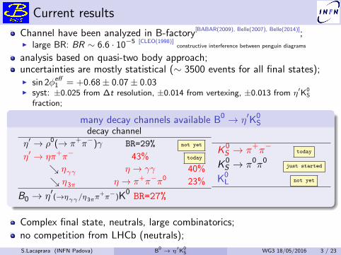
Channel have been analyzed in B-factory[BABAR(2009), Belle(2007), Belle(2014)];I large BR: BR ∼ 6.6 · 10−5 [CLEO(1998)]

constructive interference between penguin diagrams

analysis based on quasi-two body approach;uncertainties are mostly statistical (∼ 3500 events for all final states);I sin 2φeff

1 = +0.68± 0.07± 0.03I syst: ±0.025 from ∆t resolution, ±0.014 from vertexing, ±0.013 from η′K0

S

fraction;

many decay channels available B0 → η′K0S

decay channel

η′ → ρ0(→ π+π−)γ BR=29% not yet

η′ → ηπ+π− 43% today

↘ ηγγ η → γγ 40%

↘ η3π η → π+π−π0 23%

B0 → η′(→ηγγ /η3ππ+π−

)K0BR=27%

K 0S → π+π− today

K 0S → π0π0

just started

K0L not yet

Complex final state, neutrals, large combinatorics;

no competition from LHCb (neutrals);


′K

0S WG3 18/05/2016 3 / 23

Selection

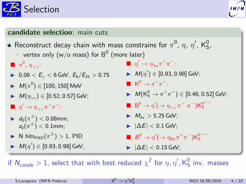
candidate selection: main cuts

Reconstruct decay chain with mass constrains for π0, η, η′, K0S,

I vertex only (w/o mass) for B0 (more later)

� π0, ηγγ :

I 0.06 < Eγ < 6 GeV, E9/E25 > 0.75

I M(π0) ∈ [100, 150] MeV

I M(ηγγ) ∈ [0.52, 0.57] GeV;

� η′ → ηγγπ+π−:

I d0(π±) < 0.08mm;z0(π±) < 0.1mm;

I N hitsPXD (π±) > 1, PID

I M(η′) ∈ [0.93, 0.98] GeV;

� η′ → η3ππ+π−:

I M(η′) ∈ [0.93, 0.98] GeV;

� K0 → π+π−:

I M(K0S → π+π−) ∈ [0.48, 0.52] GeV;

� B0 → η′(→ ηγγπ+ π−)K0

S+−

I Mbc > 5.25 GeV;

I |∆E | < 0.1 GeV;

� B0 → η′(→ η3ππ+π−)K0

S+−

I |∆E | < 0.15 GeV;

if Ncands > 1, select that with best reduced χ2 for η, η′,K0S inv. masses


′K

0S WG3 18/05/2016 4 / 23

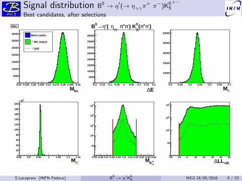
Signal distribution B0 → η′(→ ηγγπ+ π−)K0

S

+−

Best candidates, after selections

bcM5.25 5.255 5.26 5.265 5.27 5.275 5.28 5.285 5.290

5000

10000

15000

20000

25000

30000

35000

Mbc

Best cands

" MC match

" SXF

Mbc

E∆0.2− 0.15− 0.1− 0.05− 0 0.05 0.1 0.15 0.20

5000

10000

15000

20000

25000

30000

35000

40000

ηM0.4 0.45 0.5 0.55 0.6 0.65 0.70

10000

20000

30000

40000

50000

'ηM0.85 0.9 0.95 1 1.05 1.1 1.150

20

40

60

80

100

120

140

160

180

200

310×

S0KM

0.45 0.46 0.47 0.48 0.49 0.5 0.51 0.52 0.53 0.54 0.551

10

210

310

410

510

/KπLL∆20− 10− 0 10 20 30 40 501

10

210

310

410

)-π+π(S

0) K-π+π γγη'( η→0B


′K

0S WG3 18/05/2016 5 / 23

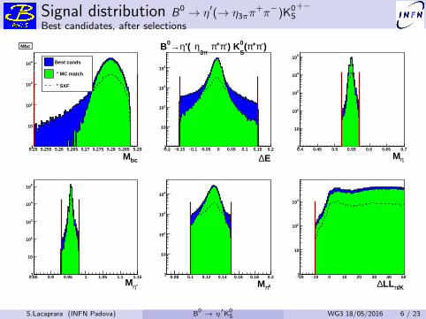
Signal distribution B0 → η′(→ η3ππ+π−)K0

S

+−

Best candidates, after selections

bcM5.25 5.255 5.26 5.265 5.27 5.275 5.28 5.285 5.291

10

210

310

410

Mbc

Best cands

" MC match

" SXF

Mbc

E∆0.2− 0.15− 0.1− 0.05− 0 0.05 0.1 0.15 0.21

10

210

310

410

ηM0.4 0.45 0.5 0.55 0.6 0.65 0.71

10

210

310

410

510

'ηM0.85 0.9 0.95 1 1.05 1.1 1.151

10

210

310

410

510

0πM0.08 0.1 0.12 0.14 0.16 0.18 0.21

10

210

310

410

/KπLL∆20− 10− 0 10 20 30 40 501

10

210

310

)-π+π(S

0) K-π+π π3

η'( η→0B


′K

0S WG3 18/05/2016 6 / 23

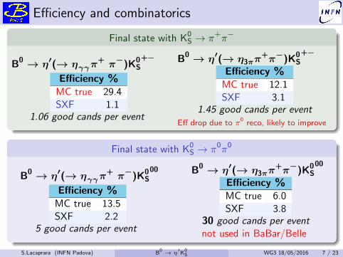
Efficiency and combinatorics

Final state with K0S → π+π−

B0 → η′(→ ηγγπ+ π−)K0

S+−

Efficiency %MC true 29.4SXF 1.1

1.06 good cands per event

B0 → η′(→ η3ππ+π−)K0

S+−


1.45 good cands per eventEff drop due to π0 reco, likely to improve

Final state with K0S → π0π0

B0 → η′(→ ηγγπ+ π−)K0

S00


5 good cands per event

B0 → η′(→ η3ππ+π−)K0

S00


30 good cands per eventnot used in BaBar/Belle


′K

0S WG3 18/05/2016 7 / 23

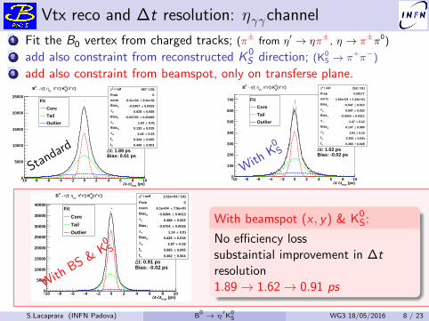
Vtx reco and ∆t resolution: ηγγchannel

1 Fit the B0 vertex from charged tracks; (π± from η′ → ηπ±, η → π±π0)

2 add also constraint from reconstructed K 0S direction; (K0

S → π+π−)

3 add also constraint from beamspot, only on transferse plane.

(ps)truet∆t-∆10− 8− 6− 4− 2− 0 2 4 6 8 10

0

5000

10000

15000

20000

25000

/ ndf 2χ 867 / 191

Prob 0

norm 8.0e+01± 6.3e+04

CBias 0.0025±0.0307 −

Cσ 0.005± 0.629

T

Bias 0.00485±0.00735 − Tσ 0.01± 1.63

OBias 0.015± 0.132

Oσ 0.03± 4.46

Cf 0.005± 0.344

Tf 0.003± 0.443

Fit

Core

Tail

Outlier

t: 1.89 ps∆Bias: 0.01 ps

)-π+π(S

0) K-π+π γγ

η'( η→0B

Standard

(ps)truet∆t-∆10− 8− 6− 4− 2− 0 2 4 6 8 10

0

100

200

300

400

500

600

700

/ ndf 2χ 253 / 191

Prob 0.00177

norm 1.24e+01± 1.54e+03

CBias 0.013±0.047 −

Cσ 0.033± 0.587

T

Bias 0.0313±0.0524 −

T

σ 0.12± 1.47

OBias 0.080± 0.107

Oσ 0.15± 3.81

Cf 0.041± 0.393

Tf 0.028± 0.393

Fit

Core

Tail

Outlier

t: 1.62 ps∆Bias: -0.02 ps

)-π+π(S

0) K-π+π γγ

η'( η→0B

WithK0S

(ps)truet∆t-∆10− 8− 6− 4− 2− 0 2 4 6 8 10

0

5000

10000

15000

20000

25000

30000

35000

40000

/ ndf 2χ 1.02e+03 / 191

Prob 0

norm 7.8e+01± 6.1e+04

CBias 0.0013±0.0399 −

Cσ 0.002± 0.488

T

Bias 0.0036±0.0704 − Tσ 0.01± 1.14

OBias 0.018± 0.429

Oσ 0.02± 2.97

Cf 0.005± 0.565

Tf 0.004± 0.362

Fit

Core

Tail

Outlier

t: 0.91 ps∆Bias: -0.02 ps

)-π+π(S

0) K-π+π γγ

η'( η→0B

WithBS &

K0S

With beamspot (x , y) & K0S:

No efficiency losssubstaintial improvement in ∆tresolution1.89→ 1.62→ 0.91 ps


′K

0S WG3 18/05/2016 8 / 23

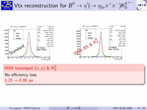
Vtx reconstruction for B0 → η′(→ η3ππ+π−)K0

S+−

(ps)truet∆t-∆10− 8− 6− 4− 2− 0 2 4 6 8 10

0

2000

4000

6000

8000

10000

12000

14000

16000

/ ndf 2χ 499 / 191

Prob 29− 2.06e

norm 5.65e+01± 3.19e+04

CBias 0.0027±0.0223 −

Cσ 0.005± 0.535

T

Bias 0.0052±0.0277 −

T

σ 0.01± 1.29

OBias 0.019± 0.266

Oσ 0.03± 3.15

Cf 0.007± 0.401

Tf 0.01± 0.46

Fit

Core

Tail

Outlier

t: 1.25 ps∆Bias: 0.02 ps

)-π+π(S

0) K-π+π π3

η'( η→0B

Standard

(ps)truet∆t-∆10− 8− 6− 4− 2− 0 2 4 6 8 10

0

2000

4000

6000

8000

10000

12000

14000

16000

18000

20000

/ ndf 2χ 629 / 191

Prob 0

norm 5.49e+01± 3.02e+04

CBias 0.002±0.036 −

Cσ 0.003± 0.445

T

Bias 0.0050±0.0562 −

T

σ 0.01± 1.07

OBias 0.021± 0.317

Oσ 0.02± 2.88

Cf 0.007± 0.565

Tf 0.006± 0.342

Fit

Core

Tail

Outlier

t: 0.88 ps∆Bias: -0.01 ps

)-π+π(S

0) K-π+π π3

η'( η→0B

WithBS &

K0S

With beamspot (x , y) & K0S:

No efficiency loss1.25→ 0.88 ps


′K

0S WG3 18/05/2016 9 / 23

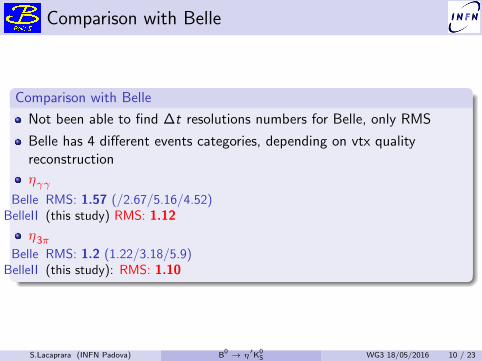
Comparison with Belle

Comparison with Belle

Not been able to find ∆t resolutions numbers for Belle, only RMS

Belle has 4 different events categories, depending on vtx qualityreconstruction

ηγγBelle RMS: 1.57 (/2.67/5.16/4.52)

BelleII (this study) RMS: 1.12

η3π

Belle RMS: 1.2 (1.22/3.18/5.9)BelleII (this study): RMS: 1.10


′K

0S WG3 18/05/2016 10 / 23

Backgrounds

Combinatorial: from continuum background e+e− → uu, dd , ss, ccI evaluated from Mbc side bands on real dataI now from MC productionI use Continuum Suppression variable

F multivariate variables sensitive to event topologyF central (signal) vs jet-like (continuum)

Peaking: any other B decays possibly with real η′ and/or K0S

I evaluated from MC of generic B0B0, B+B−

F actual B0 → η′K0 removed.

Current results based on BGx0 production, namely w/o machinebackgroundI impact of machine background under study

(almost) solved skimming problem for mixed and chargedI harder cut on skim selectionsI now L ≈ 800 fb−1 for all sources (was ≈ 200 fb−1 for mixed/charged)

Next table numbers before Continuum Suppression cut


′K

0S WG3 18/05/2016 11 / 23

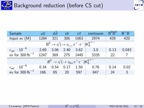
Background reduction (before CS cut)

Sample uu dd ss cc contiuum B0B0 B+B−

Input ev (M) 1284 321 306 1063 2974 429 420

B0 → η′(→ ηγγπ+ π−)K0

S

+−

εsel · 10−6 2.69 3.06 2.40 3.62 3.0 0.13 0.043

ev for 300 fb−1 1247 369 275 1445 3335 22 7

B0 → η′(→ η3ππ+π−)K0

S

+−

εsel · 10−6 0.34 0.54 0.17 1.50 0.76 0.14 0.02

ev for 300 fb−1 166 65 20 597 847 24 3


′K

0S WG3 18/05/2016 12 / 23

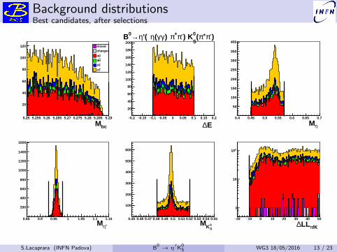
Background distributionsBest candidates, after selections

5.25 5.255 5.26 5.265 5.27 5.275 5.28 5.285 5.29

20

40

60

80

100

120

bcM

mixedcharged

uuddss

cc

0.2− 0.15− 0.1− 0.05− 0 0.05 0.1 0.15 0.2

20

40

60

80

100

120

140

160

180

200

E∆0.4 0.45 0.5 0.55 0.6 0.65 0.7

50

100

150

200

250

300

350

400

ηM

0.85 0.9 0.95 1 1.05 1.1 1.15

200

400

600

800

1000

1200

1400

1600

'ηM0.45 0.46 0.47 0.48 0.49 0.5 0.51 0.52 0.53 0.54 0.55

100

200

300

400

500

600

S0KM

20− 10− 0 10 20 30 40 50

1

10

210

/KπLL∆

)-π+π(S

0) K-π+π) γγ(η'( η→0B


′K

0S WG3 18/05/2016 13 / 23

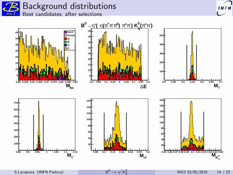
Background distributionsBest candidates, after selections

5.25 5.255 5.26 5.265 5.27 5.275 5.28 5.285 5.29

5

10

15

20

25

30

35

40

bcM

mixedcharged

uuddsscc

0.2− 0.15− 0.1− 0.05− 0 0.05 0.1 0.15 0.2

5

10

15

20

25

30

35

40

45

E∆0.4 0.45 0.5 0.55 0.6 0.65 0.7

100

200

300

400

500

ηM

0.85 0.9 0.95 1 1.05 1.1 1.15

100

200

300

400

500

600

700

'ηM0.08 0.1 0.12 0.14 0.16 0.18 0.2

20

40

60

80

100

120

140

160

0πM0.45 0.46 0.47 0.48 0.49 0.5 0.51 0.52 0.53 0.54 0.55

20

40

60

80

100

120

140

160

180

S0K

M

)-π+π(S

0) K-π+π) 0π-π+π(η'( η→0B


′K

0S WG3 18/05/2016 14 / 23

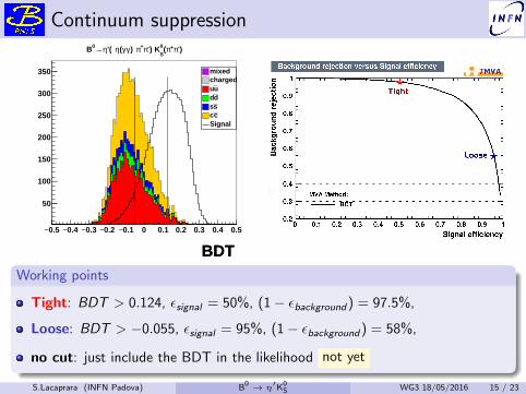
Continuum suppression

0.5− 0.4− 0.3− 0.2− 0.1− 0 0.1 0.2 0.3 0.4 0.5

50

100

150

200

250

300

350

BDTBDT

mixedcharged

uuddsscc

Signal

)-π+π(S

0) K-π+π) γγ(η'( η→0B

Signal efficiency

0 0.1 0.2 0.3 0.4 0.5 0.6 0.7 0.8 0.9 1

Ba

ck

gro

un

d r

eje

cti

on

0.2

0.3

0.4

0.5

0.6

0.7

0.8

0.9

1

MVA Method:

BDT

Background rejection versus Signal efficiency

Working points

Tight: BDT > 0.124, εsignal = 50%, (1− εbackground ) = 97.5%,

Loose: BDT > −0.055, εsignal = 95%, (1− εbackground ) = 58%,

no cut: just include the BDT in the likelihood not yet


′K

0S WG3 18/05/2016 15 / 23

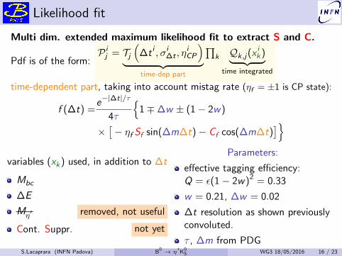
Likelihood fit

Multi dim. extended maximum likelihood fit to extract S and C.

Pdf is of the form:P i

j = Tj

(∆t i , σi

∆t , ηiCP

)︸︷︷︸

time-dep part

∏k Qk,j (x

ik )︸︷︷︸

time integrated

time-dependent part, taking into account mistag rate (ηf = ±1 is CP state):

f (∆t) =e−|∆t|/τ

4τ

{1∓∆w ± (1− 2w)

×[− ηf Sf sin(∆m∆t)− Cf cos(∆m∆t)

]}variables (xk ) used, in addition to ∆t

Mbc

∆E

Mη′ removed, not useful

Cont. Suppr. not yet

Parameters:

effective tagging efficiency:Q = ε(1− 2w)2 = 0.33

w = 0.21, ∆w = 0.02

∆t resolution as shown previouslyconvoluted.

τ , ∆m from PDGS.Lacaprara (INFN Padova) B

0 → η′K

0S WG3 18/05/2016 16 / 23

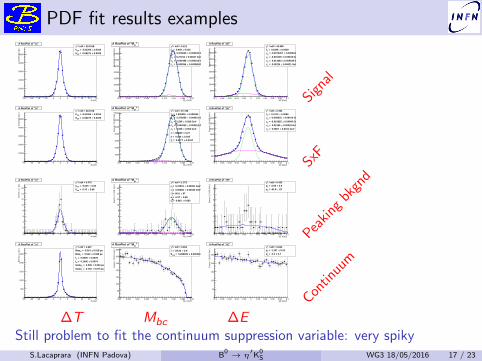
PDF fit results examples

t (ps)∆25− 20− 15− 10− 5− 0 5 10 15 20 25

Eve

nts

/ ( 1

ps

)

0

10000

20000

30000

40000

50000

t"∆A RooPlot of " / ndf = 224.5182χ

0.0014± = -2.51264 CPC

0.0039± = -0.06275 CPS

t"∆A RooPlot of "

(GeV)bcM5.25 5.255 5.26 5.265 5.27 5.275 5.28 5.285 5.29

Eve

nts

/ ( 0

.001

GeV

)

0

5000

10000

15000

20000

25000

30000

35000

"bcA RooPlot of "M / ndf = 5.2122χ

0.015± = 0.949 Cf 0.000025 GeV± = 5.279630

Cµ

0.00027 GeV± = 5.27733 T

µ 0.000012 GeV± = 0.002488 Cσ 0.000089 GeV± = 0.003056 Tσ

"bcA RooPlot of "M

E (GeV)∆0.1− 0.08− 0.06− 0.04− 0.02− 0 0.02 0.04 0.06 0.08 0.1

Eve

nts

/ ( 0

.005

GeV

)

0

5000

10000

15000

20000

25000

30000

35000

E"∆A RooPlot of " / ndf = 42.9652χ

0.0029± = 0.8108 Cf 0.000034 GeV± = -0.0072407

Cµ

0.00019 GeV± = -0.015109 T

µ 0.000039 GeV± = 0.011661 Cσ

0.00021 GeV± = 0.03224 Tσ

E"∆A RooPlot of "

Signal

t (ps)∆25− 20− 15− 10− 5− 0 5 10 15 20 25

Eve

nts

/ ( 1

ps

)

0

10000

20000

30000

40000

50000


0.0014± = -2.51264 CPC

0.0039± = -0.06275 CPS

t"∆A RooPlot of "

(GeV)bcM5.25 5.255 5.26 5.265 5.27 5.275 5.28 5.285 5.29

Eve

nts

/ ( 0

.001

GeV

)

0

1000

2000

3000

4000

5000

6000

7000


0.000050± = 1.000000 Cf 0.000015 GeV± = 5.279280

Cµ

0.026 GeV± = 5.289 T

µ 0.000012 GeV± = 0.003023 Cσ

0.052 GeV± = 0.009 Tσ

0.27± = -90.000 ξ 0.035±n = 0.545

0.0017± = 0.9477 Pf

"bcA RooPlot of "M

E (GeV)∆0.1− 0.08− 0.06− 0.04− 0.02− 0 0.02 0.04 0.06 0.08 0.1

Eve

nts

/ ( 0

.005

GeV

)

0

500

1000

1500

2000

2500

3000

3500

4000


0.0060± = 0.4112 Cf 0.00014 GeV± = -0.008252

Cµ

0.00060 GeV± = -0.010825 T

µ 0.00018 GeV± = 0.01380 Cσ

0.0011 GeV± = 0.0687 Tσ

E"∆A RooPlot of "

SxF

t (ps)∆25− 20− 15− 10− 5− 0 5 10 15 20 25

Eve

nts

/ ( 1

ps

)

0

2

4

6

8

10

12

14

16


0.32± = -0.015 CPC

0.66± = 0.76 CPS

t"∆A RooPlot of "

(GeV)bcM5.25 5.255 5.26 5.265 5.27 5.275 5.28 5.285 5.29

Eve

nts

/ ( 0

.001

GeV

)

0

2

4

6

8

10

12

14

16


0.00051 GeV± = 5.27876 µ 0.00044 GeV± = 0.00282 σ

87± = -90.0 ξ 0.59±n = 0.37

0.083± = 0.862 Pf

"bcA RooPlot of "M

E (GeV)∆0.1− 0.08− 0.06− 0.04− 0.02− 0 0.02 0.04 0.06 0.08 0.1

Eve

nts

/ ( 0

.005

GeV

)

0

1

2

3

4

5

6

7

8


2.0± = -2.68 1

p

23± = -61.8 2

p

E"∆A RooPlot of "

Peaki

ngbkg

nd

t (ps)∆25− 20− 15− 10− 5− 0 5 10 15 20 25

Eve

nts

/ ( 1

ps

)

0

500

1000

1500

2000

2500


0.018 ps± = 0.014 CBias

0.069 ps± = 0.512 TBias

0.0078± = 0.5000 Cf

0.0074± = 0.1406 Of

0.023 ps± = 0.539 CScale

0.074 ps± = 2.745 TScale

t"∆A RooPlot of "

(GeV)bcM5.25 5.255 5.26 5.265 5.27 5.275 5.28 5.285 5.29

Eve

nts

/ ( 0

.001

GeV

)

0

50

100

150

200

250

300

350


2.9± = -29.23 ξ 0.000031 GeV± = 5.286930 endE

"bcA RooPlot of "M

E (GeV)∆0.1− 0.08− 0.06− 0.04− 0.02− 0 0.02 0.04 0.06 0.08 0.1

Eve

nts

/ ( 0

.005

GeV

)

0

50

100

150

200

250


0.19± = -1.107 1

p

3.7± = 2.3 2

p

E"∆A RooPlot of "

Contin

uum

∆T Mbc ∆EStill problem to fit the continuum suppression variable: very spiky


′K

0S WG3 18/05/2016 17 / 23

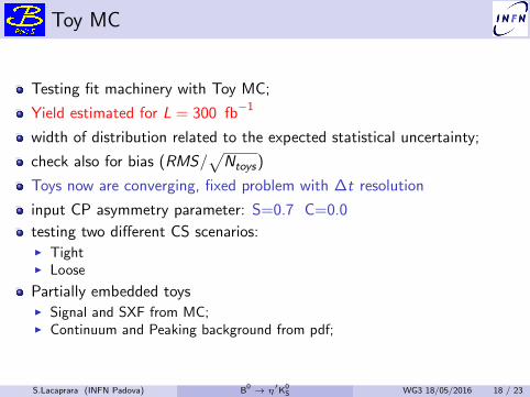
Toy MC

Testing fit machinery with Toy MC;

Yield estimated for L = 300 fb−1

width of distribution related to the expected statistical uncertainty;

check also for bias (RMS/√Ntoys)

Toys now are converging, fixed problem with ∆t resolution

input CP asymmetry parameter: S=0.7 C=0.0

testing two different CS scenarios:I TightI Loose

Partially embedded toysI Signal and SXF from MC;I Continuum and Peaking background from pdf;


′K

0S WG3 18/05/2016 18 / 23

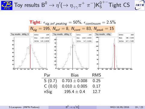
Toy results B0 → η′(→ ηγγπ+ π−)K0

S+−

Tight CS

Tight: εsig ,sxf ,peaking = 50%, εcontinuum = 2.5%

Nsig = 195, Nsxf = 8, Ncont = 83, Npeak = 15

0.2− 0 0.2 0.4 0.6 0.8 1 1.2 1.4 1.60

10

20

30

40

50

60

70

Toy results - dtSig_S Entries 1000

Mean 0.0079± 0.703

Std Dev 0.00559± 0.25

Toy results - dtSig_S

0.6− 0.4− 0.2− 0 0.2 0.4 0.60

10

20

30

40

50

60

70

80

Toy results - dtSig_C Entries 1000

Mean 0.00539± 0.0103

Std Dev 0.00381± 0.17

Toy results - dtSig_C

0 50 100 150 200 250 300 350 4000

20

40

60

80

100

120

140

Toy results - nSig Entries 1000

Mean 0.403± 195

Std Dev 0.285± 12.7

Toy results - nSig

Par Bias RMS

S (0.7) 0.703± 0.008 0.25C (0.0) 0.010± 0.005 0.17nSig 195.4± 0.4 12.7


′K

0S WG3 18/05/2016 19 / 23

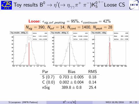
Toy results B0 → η′(→ ηγγπ+ π−)K0

S+−

Loose CS

Loose: εsig ,sxf ,peaking = 95%, εcontinuum = 42%


0.2− 0 0.2 0.4 0.6 0.8 1 1.2 1.4 1.60

10

20

30

40

50

60

70

80


Mean 0.00572± 0.703

Std Dev 0.00405± 0.181


0.6− 0.4− 0.2− 0 0.2 0.4 0.60

10

20

30

40

50

60

70

80

90


Mean 0.00441± 0.00198

Std Dev 0.00312± 0.139


0 100 200 300 400 500 600 700 8000

20

40

60

80

100

120


Mean 0.804± 390

Std Dev 0.568± 25.4

Toy results - nSig

Par Bias RMS

S (0.7) 0.703± 0.005 0.18C (0.0) 0.002± 0.004 0.14nSig 389.8± 0.8 25.4


′K

0S WG3 18/05/2016 20 / 23

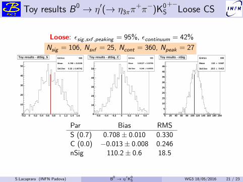
Toy results B0 → η′(→ η3ππ+π−)K0

S+−

Loose CS

Loose: εsig ,sxf ,peaking = 95%, εcontinuum = 42%


0.2− 0 0.2 0.4 0.6 0.8 1 1.2 1.4 1.60

10

20

30

40

50


Mean 0.0105± 0.708

Std Dev 0.00742± 0.33


0.6− 0.4− 0.2− 0 0.2 0.4 0.60

10

20

30

40

50


Mean 0.00785± 0.00127

Std Dev 0.00555± 0.246


0 20 40 60 80 100 120 140 160 180 2000

5

10

15

20

25

30

35

40

45


Mean 0.587± 110

Std Dev 0.415± 18.5

Toy results - nSig

Par Bias RMS

S (0.7) 0.708± 0.010 0.330C (0.0) −0.013± 0.008 0.246nSig 110.2± 0.6 18.5


′K

0S WG3 18/05/2016 21 / 23

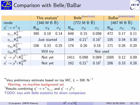
Comparison with Belle/BaBar

This analysis? Belle[Belle(2014)] BaBar[BABAR(2009)]

mode (340 M B B) (772 M B B) (467 M B B)

η′ → π±η Nsig σS σC Nsig σS σC Nsig σC σS

ηγγK0S

+−390 0.18 0.14 648 0.15 0.098 472 0.17 0.11

ηγγK0S

00Just started 104 0.21† 0.18† 105 0.34 0.30

η3πK0S

+−106 0.33 0.25 174 0.26 0.18 171 0.26 0.20

η3πK0S

00Will try Not used

η′ → ρ0γK0S

+−Not yet 1411 0.098 0.069 1005 0.12 0.09

η′ → ρ0γK0S

00Not yet 162 0.21† 0.18† 206 0.33 0.26

?Very preliminary estimate based on toy MC, L = 300 fb−1

Warning: no machine background yet†Results combining η′ → π±ηγγ and η′ → ρ0γTODO: toys with Belle statistics for direct comparison


′K

0S WG3 18/05/2016 22 / 23

Summary

First presentation on sensitivity study for ��CP in B0 → η ′K0S channel;

not complete, yet, but preliminary results are encouraging;I comparison with Belle and BaBar results looks fine;

many thing to do:I complete K0

S → π+π− channels;I study K0

S → π0π0 final states;

I add η′ → ρ0γK0S

+−/K0

S

00channel;

I systematics uncertainties evaluation;I documentationI . . .

More results (and work) for next B2TIP workshop.


′K

0S WG3 18/05/2016 23 / 23

Additional stuff

Additional or backup slides


′K

0S WG3 18/05/2016 1 / 16

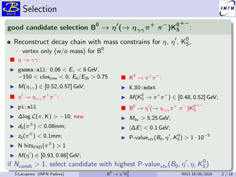
Selection

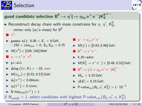
good candidate selection B0 → η′(→ ηγγπ+ π−)K0

S+−

:

Reconstruct decay chain with mass constrains for η, η′, K0S,

I vertex only (w/o mass) for B0

� η → γγ :

I gamma:all: 0.06 < Eγ < 6 GeV,−150 < clustime < 0, E9/E25 > 0.75

I M(ηγγ) ∈ [0.52, 0.57] GeV;

� η′ → ηγγπ+π−:

I pi:all

I ∆logL(π,K) > −10; new

I d0(π±) < 0.08mm;

I z0(π±) < 0.1mm;

I N hitsPXD (π±) > 1

I M(η′) ∈ [0.93, 0.98] GeV;

� K0 → π+π−:

I K S0:mdst

I M(K0S → π+π−) ∈ [0.48, 0.52] GeV;

� B0 → η′(→ ηγγπ+ π−)K0

S+−

I Mbc > 5.25 GeV;

I |∆E | < 0.1 GeV;

I P-valuevtx (B0, η′,K 0

S ) > 1 · 10−5

if Ncands > 1, select candidate with highest P-valuevtx (B0, η′, η,K 0

S )


′K

0S WG3 18/05/2016 2 / 16

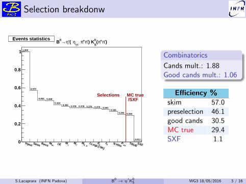
Selection breakdonw

1.000

0.570

0.463 0.458

0.4140.392 0.378 0.378 0.376 0.370 0.361

0.3360.305 0.294

0.011

InputSkim Reco bc

M E∆ ηM

'ηM

K_SM

/K)πLogL(

∆0

d0

z N Hits vtxP TRUE

SXF0

0.2

0.4

0.6

0.8

1

Events statistics

Selections MC true /SXF

)-π+π(S

0) K-π+π γγ

η'( η→0BEvents statistics

Combinatorics

Cands mult.: 1.88Good cands mult.: 1.06

Efficiency %skim 57.0preselection 46.1good cands 30.5MC true 29.4SXF 1.1


′K

0S WG3 18/05/2016 3 / 16

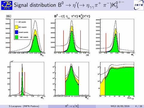
Signal distribution B0 → η′(→ ηγγπ+ π−)K0

S+−

bcM5.25 5.255 5.26 5.265 5.27 5.275 5.28 5.285 5.290

10000

20000

30000

40000

50000

60000

70000

Mbc

All cands

MC match

Good cands

" MC match

Mbc

E∆0.2− 0.15− 0.1− 0.05− 0 0.05 0.1 0.15 0.20

10000

20000

30000

40000

50000

60000

ηM0.4 0.45 0.5 0.55 0.6 0.65 0.70

10000

20000

30000

40000

50000

60000

70000

80000

90000

'ηM0.85 0.9 0.95 1 1.05 1.1 1.150

50

100

150

200

250

310×

S0

KM

0.45 0.46 0.47 0.48 0.49 0.5 0.51 0.52 0.53 0.54 0.551

10

210

310

410

510

/KπLL∆20− 10− 0 10 20 30 40 501

10

210

310

410

)-π+π(S

0) K-π+π γγη'( η→0B


′K

0S WG3 18/05/2016 4 / 16

Selection

good candidate selection B0 → η′(→ η3ππ+π−)K0

S+−

:

Reconstruct decay chain with mass constrains for η, η′, K0S,

I vertex only (w/o mass) for B0

� π0:

I gamma:all: 0.06 < Eγ < 6 GeV,−150 < clustime < 0, E9/E25 > 0.75

I M(π0) ∈ [100, 150] MeV

� η → π+π−π0:

I pi:all

I ∆logL(π,K) > −10; new

I M(η3π) ∈ [0.52, 0.57] GeV;

I d0(π±) < 0.08mm;

I z0(π±) < 0.1mm;

I N hitsPXD (π±) > 1

� η′ → η3ππ+π−:

I M(η′) ∈ [0.93, 0.98] GeV;

� K0 → π+π−:

I K S0:mdst

I M(K0S → π+π−) ∈ [0.48, 0.52] GeV;

� B0 → η′(→ η3ππ+π−)K0

S+−

I Mbc > 5.25 GeV;

I |∆E | < 0.15 GeV;

I P-valuevtx (B0, η′,K 0

S ) > 1 · 10−5

if Ncands > 1, select candidate with highest P-valuevtx (B0, η′, η,K 0

S )


′K

0S WG3 18/05/2016 5 / 16

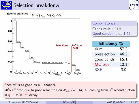
Selection breakdonw

1.000

0.572

0.464

0.398

0.265

0.1870.170 0.164 0.164 0.163 0.162 0.161 0.158 0.151

0.121

0.030

InputSkim Reco bc

M E∆ ηM

'ηM

0πM

K_SM

/K)πLogL(

∆0

d0

z N Hits vtxP TRUE

SXF0

0.2

0.4

0.6

0.8

1

Events statistics

Selections MC true /SXF

)-π+π(S

0) K-π+π π3

η'( η→0BEvents statistics

Combinatorics

Cands mult.: 21.5Good cands mult.: 1.45

Efficiency %skim 57.2preselection 46.2good cands 15.1MC true 12.1SXF 3.0

Reco eff is as good as ηγγ channel.

50% eff drop due to poor resolution on Mbc , ∆E , Mη all coming from π0 reconstruction

in η → π+π−π0 decay


′K

0S WG3 18/05/2016 6 / 16

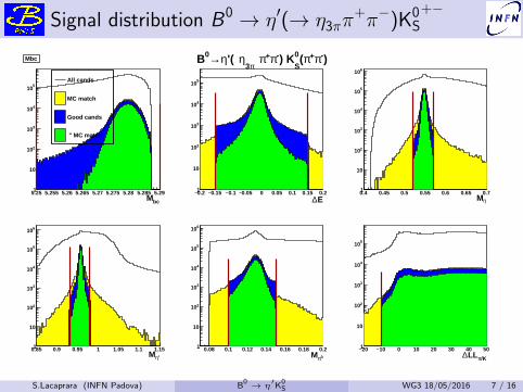
Signal distribution B0 → η′(→ η3ππ+π−)K0

S+−

bcM5.25 5.255 5.26 5.265 5.27 5.275 5.28 5.285 5.291

10

210

310

410

510

Mbc

All cands

MC match

Good cands

" MC match

Mbc

E∆0.2− 0.15− 0.1− 0.05− 0 0.05 0.1 0.15 0.21

10

210

310

410

510

ηM0.4 0.45 0.5 0.55 0.6 0.65 0.71

10

210

310

410

510

610

'ηM0.85 0.9 0.95 1 1.05 1.1 1.151

10

210

310

410

510

610

0πM0.08 0.1 0.12 0.14 0.16 0.18 0.21

10

210

310

410

510

610

/KπLL∆20− 10− 0 10 20 30 40 501

10

210

310

410

510

)-π+π(S

0) K-π+π π3

η'( η→0B


′K

0S WG3 18/05/2016 7 / 16

Final state with K0S → π0π0

A very preliminary study has been performed also with K0S → π0π0

decay.

The efficiency is roughly 12 of that of the corresponding

K0S → π+π−channel.

events combinatorics is larger for ηγγ (∼ 5 cands/ev), huge for η3π

(∼ 30 cand/ev)

SXF ∼stable, but fractionally larger due to lower signal efficiency.

∆t resolution is same as for K0S → π+π−.

B0 → η′(→ ηγγπ+ π−)K0

S

00


B0 → η′(→ η3ππ+π−)K0

S

00


not used in Belle


′K

0S WG3 18/05/2016 8 / 16

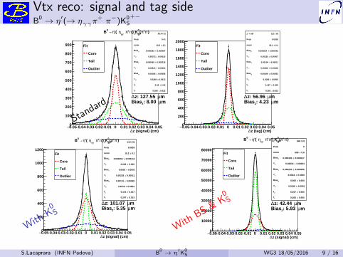
Vtx reco: signal and tag sideB0 → η′(→ ηγγπ

+ π−)K0S

+−

z (signal) (cm)∆0.05− 0.04− 0.03− 0.02− 0.01− 0 0.01 0.02 0.03 0.04 0.050

100

200

300

400

500

600

700

800

900

/ ndf 2χ 93.4 / 91

Prob 0.41

norm 0.1± 15.6

C

Bias 0.000097± 0.000393

C

σ 0.00015± 0.00371

T

Bias 0.000216± 0.000459

T

σ 0.00054± 0.00924

O

Bias 0.00056± 0.00166

O

σ 0.0013± 0.0269

Cf 0.03± 0.33

Tf 0.022± 0.368

Fit

Core

Tail

Outlier

mµz: 127.55 ∆mµ: 8.00 zBias

z (tag) (cm)∆0.05− 0.04− 0.03− 0.02− 0.01− 0 0.01 0.02 0.03 0.04 0.050

200

400

600

800

1000

1200

1400

1600

1800

2000

/ ndf 2χ 121 / 91

Prob 0.0208

norm 0.1± 16.1

C

Bias 0.000043± 0.000524

C

σ 0.00007± 0.00235

T

Bias 0.00011± 0.00104

T

σ 0.00026± 0.00605

O

Bias 0.00052±0.00199 −

O

σ 0.0006± 0.0185

Cf 0.025± 0.497

Tf 0.021± 0.383

Fit

Core

Tail

Outlier

mµz: 56.96 ∆mµ: 4.23 zBias

)-π+π(S

0) K-π+π γγ

η'( η→0B

Standard

z (signal) (cm)∆0.05− 0.04− 0.03− 0.02− 0.01− 0 0.01 0.02 0.03 0.04 0.050

200

400

600

800

1000

1200

/ ndf 2χ 110 / 91

Prob 0.0839

norm 0.1± 15.2

C

Bias 0.000111± 0.000355

C

σ 0.000± 0.006

T

Bias 0.0001± 0.0002

T

σ 0.00011± 0.00228

O

Bias 0.00035± 0.00101

O

σ 0.0004± 0.0212

Cf 0.017± 0.472

Tf 0.013± 0.207

Fit

Core

Tail

Outlier

mµz: 101.07 ∆mµ: 5.35 zBias

z (tag) (cm)∆0.05− 0.04− 0.03− 0.02− 0.01− 0 0.01 0.02 0.03 0.04 0.050

200

400

600

800

1000

1200

1400

1600

1800

/ ndf 2χ 117 / 91

Prob 0.0348

norm 0.1± 15.5

CBias 0.00004± 0.00052

C

σ 0.00007± 0.00233

T

Bias 0.00011± 0.00104

Tσ 0.00025± 0.00604

OBias 0.00054±0.00211 −

O

σ 0.0006± 0.0186

Cf 0.02± 0.49

Tf 0.02± 0.39

Fit

Core

Tail

Outlier

mµz: 57.22 ∆mµ: 4.09 zBias

)-π+π(S

0) K-π+π γγ

η'( η→0B

WithK0S

z (signal) (cm)∆0.05− 0.04− 0.03− 0.02− 0.01− 0 0.01 0.02 0.03 0.04 0.050

10000

20000

30000

40000

50000

60000

70000

80000

/ ndf 2χ 940 / 91

Prob 0

norm 0.8± 609

C

Bias 0.000017± 0.000435

C

σ 0.00004± 0.00534

T

Bias 0.000006± 0.000233

T

σ 0.0000± 0.0024

O

Bias 0.000± 0.005

O

σ 0.0001± 0.0156

Cf 0.005± 0.357

Tf 0.005± 0.583

Fit

Core

Tail

Outlier

mµz: 42.44 ∆mµ: 5.93 zBias

z (tag) (cm)∆0.05− 0.04− 0.03− 0.02− 0.01− 0 0.01 0.02 0.03 0.04 0.050

10000

20000

30000

40000

50000

60000

70000

/ ndf 2χ 1.02e+03 / 91

Prob 0

norm 0.8± 608

C

Bias 0.000007± 0.000498

C

σ 0.00001± 0.00245

T

Bias 0.00002± 0.00103

T

σ 0.00005± 0.00625

O

Bias 0.00008±0.00122 −

O

σ 0.0001± 0.0179

Cf 0.004± 0.527

Tf 0.003± 0.356

Fit

Core

Tail

Outlier

mµz: 56.17 ∆mµ: 4.88 zBias

)-π+π(S

0) K-π+π γγ

η'( η→0B

WithBS &

K0S


′K

0S WG3 18/05/2016 9 / 16

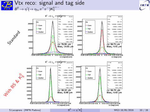
Vtx reco: signal and tag sideB0 → η′(→ η3ππ

+π−)K0S

+−

z (signal) (cm)∆0.05− 0.04− 0.03− 0.02− 0.01− 0 0.01 0.02 0.03 0.04 0.050

5000

10000

15000

20000

25000

/ ndf 2χ 774 / 91

Prob 0

norm 0.6± 318

C

Bias 0.000025± 0.000762

C

σ 0.000± 0.006

T

Bias 0.000016± 0.000333

T

σ 0.00002± 0.00242

O

Bias 0.00008± 0.00432

O

σ 0.0001± 0.0174

Cf 0.004± 0.465

Tf 0.003± 0.296

Fit

Core

Tail

Outlier

mµz: 76.55 ∆mµ: 14.81 zBias

z (tag) (cm)∆0.05− 0.04− 0.03− 0.02− 0.01− 0 0.01 0.02 0.03 0.04 0.050

5000

10000

15000

20000

25000

30000

35000

/ ndf 2χ 674 / 91

Prob 0

norm 0.6± 319

C

Bias 0.000010± 0.000499

C

σ 0.00002± 0.00245

T

Bias 0.000027± 0.000983

T

σ 0.00007± 0.00616

O

Bias 0.00011±0.00148 −

O

σ 0.0001± 0.0179

Cf 0.006± 0.511

Tf 0.005± 0.369

Fit

Core

Tail

Outlier

mµz: 56.71 ∆mµ: 4.41 zBias

)-π+π(S

0) K-π+π π3

η'( η→0B

Stan

dard

z (signal) (cm)∆0.05− 0.04− 0.03− 0.02− 0.01− 0 0.01 0.02 0.03 0.04 0.050

5000

10000

15000

20000

25000

30000

35000

40000

45000

/ ndf 2χ 1.34e+04 / 91

Prob 0

norm 0.5± 301

C

Bias 0.00004± 0.00112

C

σ 0.00006± 0.00435

T

Bias 0.000007± 0.000199

T

σ 0.00001± 0.00205

O

Bias 0.000± 0.005

O

σ 0.0001± 0.0142

Cf 0.008± 0.285

Tf 0.009± 0.624

Fit

Core

Tail

Outlier

mµz: 38.10 ∆mµ: 8.98 zBias

z (tag) (cm)∆0.05− 0.04− 0.03− 0.02− 0.01− 0 0.01 0.02 0.03 0.04 0.050

5000

10000

15000

20000

25000

30000

35000

/ ndf 2χ 634 / 91

Prob 0

norm 0.5± 301

C

Bias 0.000028± 0.000995

C

σ 0.00007± 0.00619

T

Bias 0.000010± 0.000496

T

σ 0.00002± 0.00246

O

Bias 0.00012±0.00148 −

O

σ 0.0002± 0.0179

Cf 0.005± 0.366

Tf 0.006± 0.515

Fit

Core

Tail

Outlier

mµz: 56.70 ∆mµ: 4.43 zBias

)-π+π(S

0) K-π+π π3

η'( η→0B

With

BS

&K

0S


′K

0S WG3 18/05/2016 10 / 16

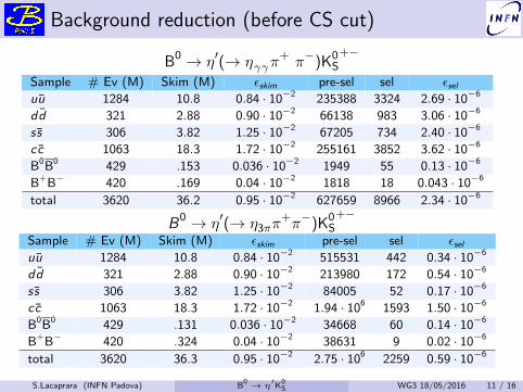
Background reduction (before CS cut)

B0 → η′(→ ηγγπ+ π−)K0

S+−

Sample # Ev (M) Skim (M) εskim pre-sel sel εsel

uu 1284 10.8 0.84 · 10−2 235388 3324 2.69 · 10−6

dd 321 2.88 0.90 · 10−2 66138 983 3.06 · 10−6

ss 306 3.82 1.25 · 10−2 67205 734 2.40 · 10−6

cc 1063 18.3 1.72 · 10−2 255161 3852 3.62 · 10−6

B0B0 429 .153 0.036 · 10−2 1949 55 0.13 · 10−6

B+B− 420 .169 0.04 · 10−2 1818 18 0.043 · 10−6

total 3620 36.2 0.95 · 10−2 627659 8966 2.34 · 10−6

B0 → η′(→ η3ππ+π−)K0

S+−

Sample # Ev (M) Skim (M) εskim pre-sel sel εsel

uu 1284 10.8 0.84 · 10−2 515531 442 0.34 · 10−6

dd 321 2.88 0.90 · 10−2 213980 172 0.54 · 10−6

ss 306 3.82 1.25 · 10−2 84005 52 0.17 · 10−6

cc 1063 18.3 1.72 · 10−2 1.94 · 106 1593 1.50 · 10−6

B0B0 429 .131 0.036 · 10−2 34668 60 0.14 · 10−6

B+B− 420 .324 0.04 · 10−2 38631 9 0.02 · 10−6

total 3620 36.3 0.95 · 10−2 2.75 · 106 2259 0.59 · 10−6


′K

0S WG3 18/05/2016 11 / 16

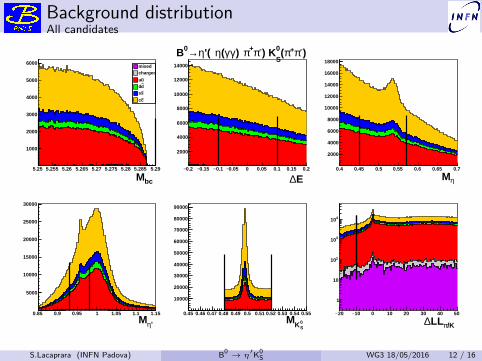
Background distributionAll candidates

5.25 5.255 5.26 5.265 5.27 5.275 5.28 5.285 5.29

1000

2000

3000

4000

5000

6000

bcM

mixedcharged

uuddss

cc

0.2− 0.15− 0.1− 0.05− 0 0.05 0.1 0.15 0.2

2000

4000

6000

8000

10000

12000

14000

E∆0.4 0.45 0.5 0.55 0.6 0.65 0.7

2000

4000

6000

8000

10000

12000

14000

16000

18000

ηM

0.85 0.9 0.95 1 1.05 1.1 1.15

5000

10000

15000

20000

25000

30000

'ηM0.45 0.46 0.47 0.48 0.49 0.5 0.51 0.52 0.53 0.54 0.55

10000

20000

30000

40000

50000

60000

70000

80000

90000

S0KM

20− 10− 0 10 20 30 40 50

1

10

210

310

410

/KπLL∆

)-π+π(S

0) K-π+π) γγ(η'( η→0B


′K

0S WG3 18/05/2016 12 / 16

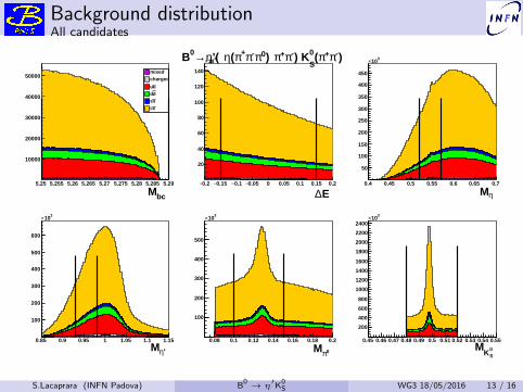
Background distributionAll candidates

5.25 5.255 5.26 5.265 5.27 5.275 5.28 5.285 5.29

10000

20000

30000

40000

50000

bcM

mixedcharged

uuddsscc

0.2− 0.15− 0.1− 0.05− 0 0.05 0.1 0.15 0.2

20

40

60

80

100

120

140

310×

E∆0.4 0.45 0.5 0.55 0.6 0.65 0.7

50

100

150

200

250

300

350

400

450

310×

ηM

0.85 0.9 0.95 1 1.05 1.1 1.15

100

200

300

400

500

600

310×

'ηM0.08 0.1 0.12 0.14 0.16 0.18 0.2

100

200

300

400

500

310×

0πM0.45 0.46 0.47 0.48 0.49 0.5 0.51 0.52 0.53 0.54 0.55

200

400

600

800

1000

1200

1400

1600

1800

2000

2200

2400

310×

S0K

M

)-π+π(S

0) K-π+π) 0π-π+π(η'( η→0B


′K

0S WG3 18/05/2016 13 / 16

Yields

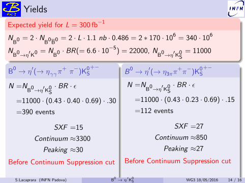
Expected yield for L = 300 fb−1

NB

0 = 2 · NB

0B

0 = 2 · L · 1.1 nb · 0.486 = 2 ∗ 170 · 106 = 340 · 106

NB

0→η′K0 = NB

0 · BR(= 6.6 · 10−5) = 22000, NB

0→η′K0S

= 11000

B0 → η′(→ ηγγπ+ π−)K0

S+−

N =NB

0→η′K0S· BR · ε

=11000 · (0.43 · 0.40 · 0.69) · .30

=390 events

SXF =15

Continuum ≈3300

Peaking ≈30

Before Continuum Suppression cut

B0 → η′(→ η3ππ+π−)K0

S+−

N =NB

0→η′K0S· BR · ε

=11000 · (0.43 · 0.23 · 0.69) · .15

=112 events

SXF =27

Continuum ≈850

Peaking ≈27

Before Continuum Suppression cut

Background


′K

0S WG3 18/05/2016 14 / 16

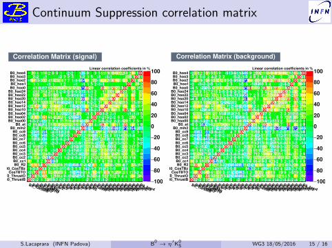
Continuum Suppression correlation matrix

100−

80−

60−

40−

20−

0

20

40

60

80

100

B0_ThrustB

B0_ThrustO

B0_CosTBTO

B0_CosTBz

B0_R2B0_cc1

B0_cc2B0_cc3

B0_cc4B0_cc5

B0_cc6B0_cc7

B0_cc8B0_cc9

B0_mm2B0_et

B0_hso00

B0_hso02

B0_hso04

B0_hso10

B0_hso12

B0_hso14

B0_hso20

B0_hso22

B0_hso24

B0_hoo0B0_hoo1

B0_hoo2B0_hoo3

B0_hoo4

B0_ThrustBB0_ThrustO

B0_CosTBTOB0_CosTBz

B0_R2B0_cc1B0_cc2B0_cc3B0_cc4B0_cc5B0_cc6B0_cc7B0_cc8B0_cc9

B0_mm2B0_et

B0_hso00B0_hso02B0_hso04B0_hso10B0_hso12B0_hso14B0_hso20B0_hso22B0_hso24B0_hoo0B0_hoo1B0_hoo2B0_hoo3B0_hoo4

Correlation Matrix (signal)

100 2 2 1 3 3119 7 2 2 1 2 1 1 2 1 2 1 2100 17 3 65 12 16 14 9 1102025 5 8 3 32 4 5 27 5 12 9 4 4 1 54 2 20 2 17100 8 61 8 24 30 25 15 183746 8 14 7 52 6 16 63 17 12 29 12 11 1 15 2 4 1 3 8100 4 2 1 9 910 8 3 5 8 742 1 3 71213 6 9 311 5 1 3 65 61 4100 9 20 24 16 216344854 101422 61 13 52 20 1 26 1417 33 1 16 31 8 2 910059 9 3 5 2 6 7 6 11 18 1 5 3 6 1 4 219 12 24 1 2059100 7 1 1 2 4 5 414 18 2 14 11 21 36 37 16 18 11 20 1 18 8 7 16 30 9 24 9 7100 3 3 5 7 822 31 4 22 6 31 44 15 24 20 6 30 25 9 2 14 25 9 16 1 3100 1 1 4101118 34 8 22 7 31 3219 18 6 2 30 1 21 2 1 2 9 1510 2 1 1100 2101219 32 13 1625 28 1730 16 3 30 2 17 2 1 1 816 2 3 1 100 4 5 617 26 16 127 22 24 12 5 5 25 7 2 2

1018 334 4 5 4 2 4100 14 22 142011 211311 11 9 6 23 1 3 22037 548 5 71010 5 100 712 16 1636 12 1724 8 911 6 20 1 42546 854 4 81112 6 710014 15 1643 29 1627 19 1010 5 21 6 1 1 5 8 7 10 314221819171412141005524 55321388411379 164 235

2 8 144214 5 18 31 34 32 26 22 16 1555100 31 4 1 83 47 9 51 11 1 86 1 41 1 8 1 3 7 122 2 2 4 8 13 16 14 16 1624 31100 5 5 6 2 2 2 2 1 29 5 7 5 1 32 52 3 61 6 14 22 22 16 1203643 4 5100 7 2 16 2 2 5 3 2 20 3 2 4 6 7 7 11 6 7252711 12 29 1 5 7100 1 2 3 1 1 1 1 5 1 5 161213 6 21 31 31 28 22 21 17 1655 83 6 2 1100 52 17 58 15 1 87 1 42 11 2 27 6313 52 11 36 44 32 17 13242732 47 2 16 2 52100 42 36 43 19 46 42 1 15

5 17 6 20 18 37 1519302411 8 1913 9 2 2 3 17 42100 16 29 20 15 15 1 13 12 12 9 1 1 16 24 18 16 12 11 9 1088 51 2 2 1 58 36 16100 41 11 75 61 34 9 29 26 5 18 20 6 5 9111041 11 2 5 15 43 29 41100 44 23 45 33 4 12 3 14 3 11 6 2 3 5 6 6 513 1 1 3 1 19 20 11 44100 3 16 22 4 111117 6 20 30 30 30 25 23 20 2179 86 29 87 46 15 75 23 3100 53 2 18 1 1 1 1 1 2 1 1 1 5 2 1 1 100 28 2

1 54 15 5 33 4 18 25 21 17 7 1 4 664 41 7 20 1 42 42 15 61 45 16 53 100 1 54 2 2 1 2 2 2 3 1 2 1 5 1 1 1 2 28 1100 1 20 4 1 16 2 8 9 1 2 2 135 8 3 5 11 15 13 34 33 22 18 2 54 1100

Linear correlation coefficients in %

100−

80−

60−

40−

20−

0

20

40

60

80

100

B0_ThrustB

B0_ThrustO

B0_CosTBTO

B0_CosTBz

B0_R2B0_cc1

B0_cc2B0_cc3

B0_cc4B0_cc5

B0_cc6B0_cc7

B0_cc8B0_cc9

B0_mm2B0_et

B0_hso00

B0_hso02

B0_hso04

B0_hso10

B0_hso12

B0_hso14

B0_hso20

B0_hso22

B0_hso24

B0_hoo0B0_hoo1

B0_hoo2B0_hoo3

B0_hoo4

B0_ThrustBB0_ThrustO

B0_CosTBTOB0_CosTBz

B0_R2B0_cc1B0_cc2B0_cc3B0_cc4B0_cc5B0_cc6B0_cc7B0_cc8B0_cc9

B0_mm2B0_et

B0_hso00B0_hso02B0_hso04B0_hso10B0_hso12B0_hso14B0_hso20B0_hso22B0_hso24B0_hoo0B0_hoo1B0_hoo2B0_hoo3B0_hoo4

Correlation Matrix (background)

100 2 3 8 10 381816 5 5 2 4 8 2 3 1 5 4 2 4 2 4 4 2 4 3 2 2100 41 88 9 26 22 13 325344649 4 5 8 45 25 10 53 30 8 21 14 5 51 3 32 3 41100 6 49 6 18 20 8 115263443 1 3 1 33 20 4 41 18 19 9 1 5 19 5 12 8 6100 9 10 4171713 5 8 863 2 1 42919 612 4 523 3 7 6 3 10 88 49 9100 19 21 13 32139454951 112121 41 3414 44 39 9 21 1720 2 36 2 33 38 9 6 10 19100571313 3 5 3 1 6 6 14 19 3 6 21 2 3 2 1 5 6 4 918 26 18 4 2157100 6 1 2 3 6 6 619 22 6 22 22 25 36 33 18 20 18 25 1 33 2 2516 22 2017 1313 6100 8 4 3 4 9 422 37 7 12 5 36 46 17 23 11 5 34 1 31 2 9 5 13 817 313 1 8100 511 1 2 515 36 8 1113 34 2221 18 3 6 31 21 2

3 11321 2 4 5100 1 1 1 20 30 13 419 30 726 18 3 5 32 2 10 5 52515 539 3 3 311 1100 2 11 418 17 19 713 151220 15 6 8 23 3 5 13

3426 845 5 6 4 1 1 2100 5 714 19 121917 161412 13 7 3 20 9 5 8 24634 49 6 9 2 1 11 5100 8 6 13 1423 8 1318 613 9 16 116 211

4943 51 3 6 4 5 4 7 810011 13 1718 1 927 3 8 8 6 16 515 1 8 4 4 1 8 11 1192215201814 611100473419 548341587583479 572 546 8 5 36321 6 22 37 36 30 17 19 13 1347100 29 17 1 80 53 10 48 7 81 44 4 9 2 8 1 221 6 6 7 8 13 19 12 14 1734 29100 55 23 812 5 13 2 3510 14 8 2 3 45 33 1 41 14 22 12 11 4 719231819 17 55100 64 4 4 8 8 7 2013 35 7 20 1 25 20 4 34 19 22 513191317 8 1 5 1 23 64100 7 2 3 3 310 18 4 21 5 10 42914 3 25 36 34 30 15 16 13 948 80 8 4 7100 69 21 55 14 5 83 3 50 1 15 4 53 4119 44 6 36 46 22 71214182734 5312 4 2 69100 57 38 33 21 55 4 63 2 34 2 30 18 6 39 21 33 1721262012 315 10 5 21 57100 13 30 28 17 37 2 36 4 8 12 9 2 18 23 18 18 15 13 6 887 48 13 8 55 38 13100 60 33 77 70 45 2 21 19 4 21 3 20 11 3 3 6 713 858 7 2 8 3 14 33 30 60100 62 31 2 69 3 58 4 14 9 5 17 2 18 5 6 5 8 3 9 634 7 3 5 21 28 33 62100 15 4 42 49 4 5 12320 1 25 34 31 32 23 20 16 1679 81 35 20 3 83 55 17 77 31 15100 2 65 3 27 2 5 3 2 5 1 1 2 3 1 5 5 101310 3 4 2 4 2100 38 3 4 51 19 7 36 6 33 31 21 10 5 9161572 44 14 35 18 50 63 37 70 69 42 65 100 5 69 3 3 5 6 2 4 2 2 2 5 2 1 5 4 8 7 4 1 2 2 3 3 38 5100 1 2 32 12 3 33 9 25 9 513 811 846 9 2 20 21 15 34 36 45 58 49 27 3 69 1100

Linear correlation coefficients in %


′K

0S WG3 18/05/2016 15 / 16

Bibliography I

[Williamson and Zupan(2006)] Alexander R. Williamson and Jure Zupan. Two body b decays with isosinglet final states in softcollinear effective theory. Phys. Rev. D, 74:014003, Jul 2006. doi: 10.1103/PhysRevD.74.014003. URLhttp://link.aps.org/doi/10.1103/PhysRevD.74.014003.

[Gronau et al.(2006)] Michael Gronau et al. Updated bounds on cp asymmetries in B0 → η

′KS and B

0 → π0

KS . Phys.Rev. D, 74:093003, Nov 2006. doi: 10.1103/PhysRevD.74.093003. URLhttp://link.aps.org/doi/10.1103/PhysRevD.74.093003.

[Belle(2014)] Belle. Measurement of time-dependent cp violation in b0 → η′k0 decays. Journal of High Energy Physics, 2014

(10):165, 2014. doi: 10.1007/JHEP10(2014)165. URL http://dx.doi.org/10.1007/JHEP10%282014%29165.

[Urquijo(2015)] Phillip Urquijo. Comparison between belle ii and lhcb physics projections. Technical ReportBELLE2-NOTE-PH-2015-004, Apr 2015.

[CLEO(1998)] CLEO. Observation of high momentum η′

production in B decays. PRL, 81:1786, 1998. doi:10.1103/PhysRevLett.81.1786. URL http://link.aps.org/doi/10.1103/PhysRevLett.81.1786.

[BABAR(2009)] BABAR. Measurement of time dependent cp asymmetry parameters in B0

meson decays to ωK0S , η

′K

0, and

π0

K0S . PRD, 79:052003, 2009. doi: 10.1103/PhysRevD.79.052003. URL

http://link.aps.org/doi/10.1103/PhysRevD.79.052003.

[Belle(2007)] Belle. Observation of time-dependent cp violation in B0 → η

′K

0decays and improved measurements of cp

asymmetries in B0 → ϕK

0, K

0S K

0S K

0S and B

0 → j/ψK0

decays. PRL, 98:031802, 2007. doi:10.1103/PhysRevLett.98.031802. URL http://link.aps.org/doi/10.1103/PhysRevLett.98.031802.


′K

0S WG3 18/05/2016 16 / 16

http://link.aps.org/doi/10.1103/PhysRevD.74.014003


http://dx.doi.org/10.1007/JHEP10%282014%29165

http://link.aps.org/doi/10.1103/PhysRevLett.81.1786


http://link.aps.org/doi/10.1103/PhysRevLett.98.031802

to (to ) Time Dependent CP-8.5-.25ex analysis - B2TIP...

Documents

Transcript of to (to ) Time Dependent CP-8.5-.25ex analysis - B2TIP...