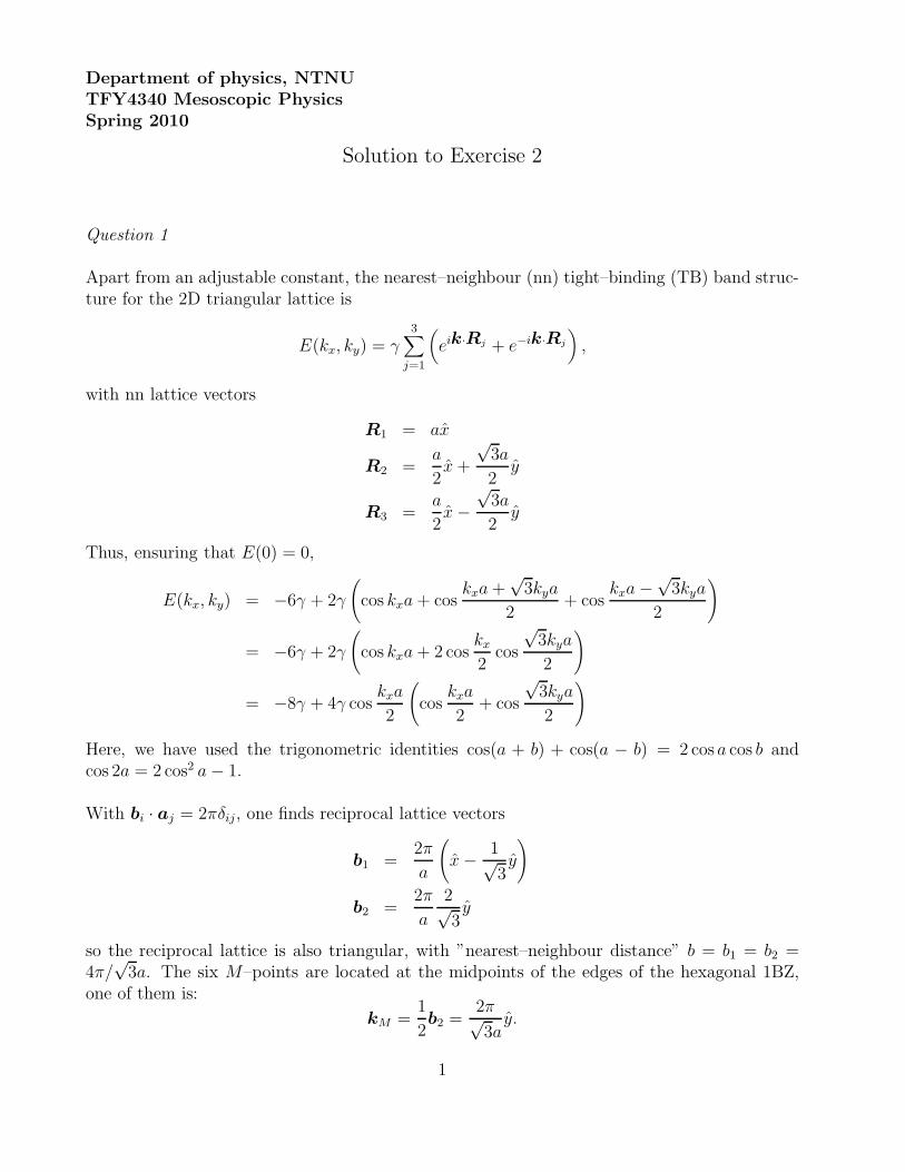
Department of physics, NTNU

TFY4340 Mesoscopic Physics

Spring 2010

Solution to Exercise 2

Question 1

Apart from an adjustable constant, the nearest–neighbour (nn) tight–binding (TB) band struc-ture for the 2D triangular lattice is

E(kx, ky) = γ3∑

j=1

(

eik·Rj + e−ik·Rj

)

,

with nn lattice vectors

R1 = ax

R2 =a

2x +

√3a

2y

R3 =a

2x −

√3a

2y

Thus, ensuring that E(0) = 0,

E(kx, ky) = −6γ + 2γ

(

cos kxa + coskxa +

√3kya

2+ cos

kxa −√

3kya

2

)

= −6γ + 2γ

(

cos kxa + 2 coskx

2cos

√3kya

2

)

= −8γ + 4γ coskxa

2

(

coskxa

2+ cos

√3kya

2

)

Here, we have used the trigonometric identities cos(a + b) + cos(a − b) = 2 cos a cos b andcos 2a = 2 cos2 a − 1.

With bi · aj = 2πδij, one finds reciprocal lattice vectors

b1 =2π

a

(

x − 1√3y

)

b2 =2π

a

2√3y

so the reciprocal lattice is also triangular, with ”nearest–neighbour distance” b = b1 = b2 =4π/

√3a. The six M–points are located at the midpoints of the edges of the hexagonal 1BZ,

one of them is:

kM =1

2b2 =

2π√3a

y.

1

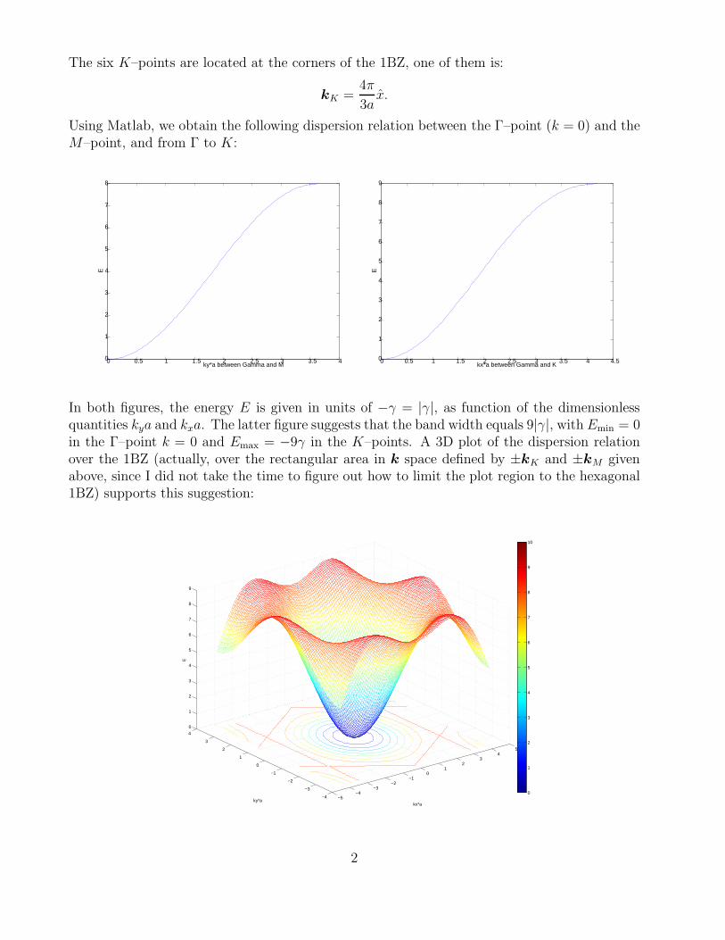
The six K–points are located at the corners of the 1BZ, one of them is:

kK =4π

3ax.

Using Matlab, we obtain the following dispersion relation between the Γ–point (k = 0) and theM–point, and from Γ to K:

0 0.5 1 1.5 2 2.5 3 3.5 40

1

2

3

4

5

6

7

8

ky*a between Gamma and M

E

0 0.5 1 1.5 2 2.5 3 3.5 4 4.50

1

2

3

4

5

6

7

8

9

kx*a between Gamma and K

E

In both figures, the energy E is given in units of −γ = |γ|, as function of the dimensionlessquantities kya and kxa. The latter figure suggests that the band width equals 9|γ|, with Emin = 0in the Γ–point k = 0 and Emax = −9γ in the K–points. A 3D plot of the dispersion relationover the 1BZ (actually, over the rectangular area in k space defined by ±kK and ±kM givenabove, since I did not take the time to figure out how to limit the plot region to the hexagonal1BZ) supports this suggestion:

−5−4

−3−2

−10

12

34

5

−4

−3

−2

−1

0

1

2

3

4

0

1

2

3

4

5

6

7

8

9

kx*aky*a

E

0

1

2

3

4

5

6

7

8

9

10

2

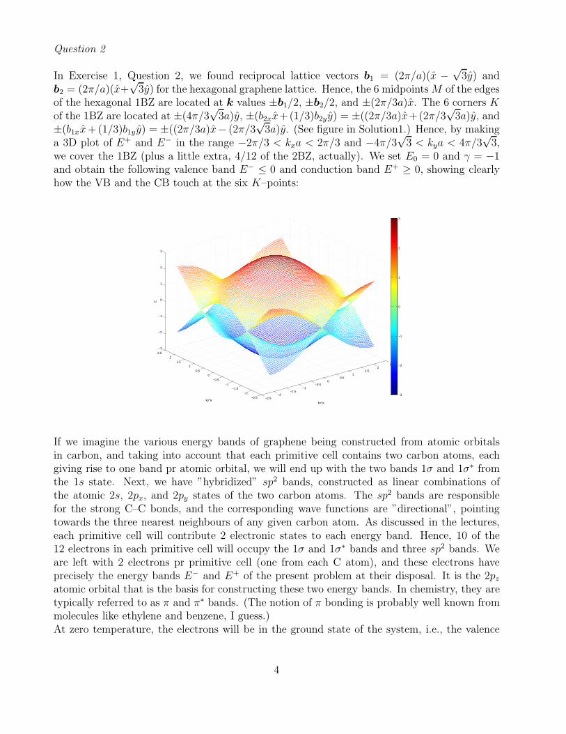
A formal way to find the band width amounts to locating the various stationary points of E(k),i.e., to find where ∇kE = 0, and insert these k values into E(k). For the 2D gradient of E tovanish, we must require both ∂E/∂kx = 0 and ∂E/∂ky = 0 simultaneously. Let α = kxa andβ = kya. Then

∂E

∂α= − sin

α

2

(

cosα

2+

1

2cos

√3β

2

)

= 0

∂E

∂β= −

√3

2cos

α

2sin

√3β

2= 0

Here, we have several solutions:

• sin(α/2) = 0 and sin(√

3β/2) = 0 yields the energy minimum Emin = 0 at the Γ–point kx = ky = 0, as well as saddle points EM = −8γ in two of the six M–points,kM = (0,±2π/

√3a)

• cos(α/2) = 0 and cos(√

3β/2) = 0 yields the remaining four saddle points EM = −8γ inkM = (±π/a,±π/

√3a)

• sin(√

3β/2) = 0 and cos(α/2) = −(1/2) cos(√

3β/2) yields the six energy maxima EK =−9γ at the K–points kK = (±4π/3a, 0) and kK = (±2π/3a,±2π/

√3a).

A 3D plot, viewed down the E–axis, and with a somewhat extended region of k–space, couldbe illustrative:

−8 −6 −4 −2 0 2 4 6 8

−6

−4

−2

0

2

4

6

ky*a

kx*a

E

0

1

2

3

4

5

6

7

8

9

10

3

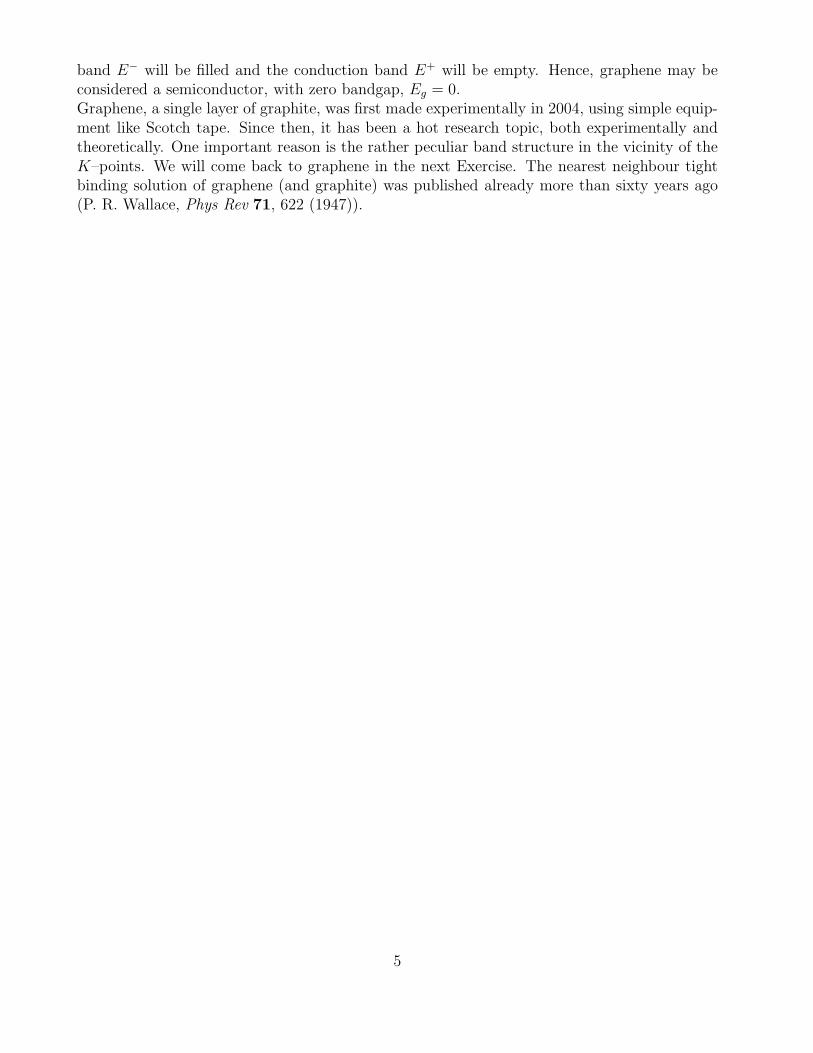
Question 2

In Exercise 1, Question 2, we found reciprocal lattice vectors b1 = (2π/a)(x −√

3y) andb2 = (2π/a)(x+

√3y) for the hexagonal graphene lattice. Hence, the 6 midpoints M of the edges

of the hexagonal 1BZ are located at k values ±b1/2, ±b2/2, and ±(2π/3a)x. The 6 corners Kof the 1BZ are located at ±(4π/3

√3a)y, ±(b2xx+(1/3)b2yy) = ±((2π/3a)x+(2π/3

√3a)y, and

±(b1xx +(1/3)b1y y) = ±((2π/3a)x− (2π/3√

3a)y. (See figure in Solution1.) Hence, by makinga 3D plot of E+ and E− in the range −2π/3 < kxa < 2π/3 and −4π/3

√3 < kya < 4π/3

√3,

we cover the 1BZ (plus a little extra, 4/12 of the 2BZ, actually). We set E0 = 0 and γ = −1and obtain the following valence band E− ≤ 0 and conduction band E+ ≥ 0, showing clearlyhow the VB and the CB touch at the six K–points:

−2.5−2

−1.5−1

−0.50

0.51

1.52

2.5

−2.5−2

−1.5−1

−0.50

0.51

1.52

2.5

−3

−2

−1

0

1

2

3

kx*aky*a

E

−3

−2

−1

0

1

2

3

If we imagine the various energy bands of graphene being constructed from atomic orbitalsin carbon, and taking into account that each primitive cell contains two carbon atoms, eachgiving rise to one band pr atomic orbital, we will end up with the two bands 1σ and 1σ∗ fromthe 1s state. Next, we have ”hybridized” sp2 bands, constructed as linear combinations ofthe atomic 2s, 2px, and 2py states of the two carbon atoms. The sp2 bands are responsiblefor the strong C–C bonds, and the corresponding wave functions are ”directional”, pointingtowards the three nearest neighbours of any given carbon atom. As discussed in the lectures,each primitive cell will contribute 2 electronic states to each energy band. Hence, 10 of the12 electrons in each primitive cell will occupy the 1σ and 1σ∗ bands and three sp2 bands. Weare left with 2 electrons pr primitive cell (one from each C atom), and these electrons haveprecisely the energy bands E− and E+ of the present problem at their disposal. It is the 2pz

atomic orbital that is the basis for constructing these two energy bands. In chemistry, they aretypically referred to as π and π∗ bands. (The notion of π bonding is probably well known frommolecules like ethylene and benzene, I guess.)At zero temperature, the electrons will be in the ground state of the system, i.e., the valence

4

band E− will be filled and the conduction band E+ will be empty. Hence, graphene may beconsidered a semiconductor, with zero bandgap, Eg = 0.Graphene, a single layer of graphite, was first made experimentally in 2004, using simple equip-ment like Scotch tape. Since then, it has been a hot research topic, both experimentally andtheoretically. One important reason is the rather peculiar band structure in the vicinity of theK–points. We will come back to graphene in the next Exercise. The nearest neighbour tightbinding solution of graphene (and graphite) was published already more than sixty years ago(P. R. Wallace, Phys Rev 71, 622 (1947)).

5