International Neutrino Summer School 2019 Group Exercise

Questions

August 5th-16th 2019

Fermilab, USA

1 Introduction to the Physics of Massive Neutrinos

Concha Gonzalez-Garcıa (YITP-Stony Brook U. & ICREA-U.Barcelona)

Maria.Gonzalez-Garcia@StonyBrook.edu

1 Show that only for a free massless fermion the chirality eigenstates are also helicity eigenstates.

2 Show that the mass matrix M of a Majorana mass

−LMaj = −1

2νL,iMij(νL,j)

c + h.c (1)

must be symmetric Mij = Mji.

3 Show that if there are N = 3 + s massive neutrinos, the leptonic mixing matrix is dimension 3 × Nand contains 3s + 3 physical angles and 2s + 1 phases for Dirac neutrinos and 3s + 3 for Majorananeutrinos

4 The decay width for β decay N → Pe−νe after integrating over the proton momentum is

dΓ = G2F cos2 θCF (E,Z)2π

∑

spin

∑

i

|Uei|2|ue(p)γ0(1− γ5)vνi(k)|2d3p

(2π)32E

d3k

(2π)32wδ(E0 − E − w) (2)

GF is Fermi constant, θC is Cabbibo’s angle, F (E,Z) a Coulomb factor, E0 is the mass differencebetween the initial and final nuclei, E is the electron energy and w is the neutrino energy. Obtain theelectron energy spectrum dΓ/dE and show that the Kurie function

K(T ) ≡

dΓ

dEC F (E,Z) |~p|E

1/2

=

√(Q− T )

∑

i

|Uei|2√

(Q− T )2 −m2i (3)

'√√√√(Q− T )

√(Q− T )2 −

∑

i

|Uei|2m2i

with Q = E0 −me y T = E −me y C = G2F cos2 θC/π

3. Show that the last equality holds only for

Q− T mi and∑

i

|Uei|2 = 1.

Plot K(T ) as a function of T for tritium (Q = 18.6 KeV) for mβ =√∑

i |Uei|2m2i = 0 and for

mβ =√∑

i |Uei|2m2i = 2.2 eV.

1

5 The charged pion decays almost 100% of the time into a muon and a (muon-type) neutrino (π+ → µ+νµ)In the reference frame where the parent pion is at rest, compute the muon energy as a function of themuon-mass (mµ), the charged pion mass (mπ), and the neutrino mass (mν). What is the absolute valueof the muon momentum (tri)vector? Numerically, what is the relative change of the muon momentumbetween mν = 0 and mν = 0.1 MeV? It is remarkable that the muon momentum from pion decay atrest has been measured at the 3.4× 10−6 level (Phys. Rev. D53, 6065 (1996)). This provides the moststringent current constraint on the muon-neutrino mass.

6 Derive the characteristic E/L in eV2 for atmospheric neutrinos, and for T2K and for Daya-Bay.

7 Show that in a disappearance experiment the survival probability for neutrinos and antineutrinos isthe same.

8 a) What is the matter potential for ντ → νs? (νs is an sterile neutrino) Compare with the potentialfor νe → νµ,τb) In the core of a supernova the matter density is ρ ∼ 1014 g/cm

3. Obtain the characteristic value for

the matter potential for forντ → νs and ντ → νs in the core of the supernova c) For what characteristicmass differences (assume Eν ∼ 10MeV ) can occur the MSW effect in such supernova? In which of thetwo channels occurs?

2 Neutrino Detection

Mark Messier (Indiana University)

messier@indiana.edu

1 Neutrino detector Livingston plot

The Livingston plot is a famous representation of progress in the construction of particle accelerators.This problem asks you to prepare a similar plot to show progress in neutrino detectors.

The first neutrino detector “El Monstro” was constructed by Reines and Cowan in the 1950s. For eachdecade since then and looking ahead into the future, find a few representative neutrino detectors andtabulate some essential data summarizing the detector technology. For example: experiment name,dates of operation, detection technology, mass (in tons), granularity (is cm). If you can find it, alsodetector cost. You are encouraged to divide the task among several groups and share your data toensure the best possible coverage.

With the data in hand, what plot or plots can you make which best represent progress in neutrinodetector technology?

2 Magnetic DUNE

Suppose you wanted to magnetize the future DUNE detector to allow for 3σ particle-by-particle electronvs. positron separation at 2 GeV. How large a field is required? Compare the energy stored in the fieldto the total energy used by the residents of Lead, SD in a single day. Suggest how you might constructsuch a field and estimate the cost of the materials required.

3 Side-by-side

Many of you no doubt work on current neutrino experiments and are expert with the simulationprograms of those experiments. Using your collaboration’s simulation tools, make event displays forthe following neutrino topologies ranging from 10 MeV to 1 TeV. To aid the problem, a text filecontaining exact neutrino interaction topologies to simulate are posted here:

https://docs.google.com/document/d/14dfU7gHvea_iLyb_TKxVGvR0B-bG-BJP96OgOHjk6H0/edit?

usp=sharing

You may choose to skip energies that are well below and/or well above the detector’s capabilities buttry to push the simulated energy as range to be as wide as possible.

2

4 Future beam

Propose a design for a near detector for a future beta beam (see, for example, Phys.Lett. B532 (2002)166-172) which is targeted toward a distant mega-ton scale water Cherenkov detector.

3 Phenomenology of Accelerator and Atmospheric Neutrinos

Concha Gonzalez-Garcıa (YITP-Stony Brook U. & ICREA-U.Barcelona)

Maria.Gonzalez-Garcia@StonyBrook.edu

1 Understanding the Atmospheric Neutrino DataRead the article “Super-Kamiokande Atmospheric Neutrino Results” by T. Toshito, hep-ex/0105023.It contains an old summary of the atmospheric neutrino data. The talk by T. Kajita, presented at theNeutrino 1998 Conference, may also prove helpful in understanding some of the Super-Kamiokandeterminology: hep-ex/981001.

1. Numerically calculate and draw histograms of the average muon neutrino survival probability inten equal-size bins of cos θx where θx is the angle between the neutrino direction and the vertical-axis at the detector’s location (θx = 0 for neutrinos coming straight from above, and θx = π forneutrinos coming from below). For simplicity, assume two flavor νµ → ντ transitions. Make onehistogram for Eν = 0.2 GeV, 2 GeV, and 20 GeV and

∆m2 = 2.5 × 10−4 eV2, 2.5 × 10−3 eV2, and 2.5 × 10−2 eV2, for a grand total of nine plots.Assume throughout that the mixing is maximal, i.e., sin 22θ = 1, and that neutrinos are produced20 km above the surface of the Earth.

2. Look at Figure 1 in the paper and compare with the results you got in part 1. Can you verifythat ∆m2 = 2.5× 10−3 eV2 and sin2 2θ = 1 is a good fit to the data (200 MeV is characteristic ofsub-GeV events, 2 GeV is typical of multi-GeV events, and 20 GeV is typical of upward stoppingmuons. The fourth category, upwardthrough- going muons, has an average energy above 100GeV.)?

3. Use the number of observed sub-GeV “e-like” events (as these seem to agree well with Monte Carlopredictions) to obtain an order of magnitude estimate of the electron neutrino flux (neutrinos perunit time and unit area). The cross section for detecting neutrinos at this energy range is roughly5 fb.

2 You want to design an accelerator neutrino oscillation experiment which is sensitive to oscillations with|∆m2 = 3× 10−3| eV2 and to the ordering. For this you want the contribution of the matter potentialto the oscillation phase to be 20% of the ∆m2

31 contribution at oscillation maximum. At what distancefrom the source do you have to put your detector?

4 Long Baseline Oscillation Experiments

Patricia Vahle (William and Mary), Jeff Hartnell (Sussex)

plvahle@wm.edu

Long-baseline neutrino oscillation experiments seek to measure CP violation, the mass hierarchy and theoctant of θ23 using electron (anti)neutrino appearance and muon (anti)neutrino disappearance in a muon(anti)neutrino beam.

The NOvA experiment has a baseline of 810 km and a peak neutrino energy of 1.9 GeV. For the pur-poses of these problems, except as noted, consider the NOvA electron (anti)neutrino appearance and muon(anti)neutrino disappearance measurements as a “counting” experiment where you consider the beam to bemonochromatic. Similarly, consider backgrounds and systematic uncertainties to be negligible compared tostatistical uncertainties, again except as noted in individual problems.

3

For this question you should consider three flavor neutrino oscillations. The standard two flavor approx-imations will be insufficient.

Consider the duration of the NOvA experiment as an exposure of 36× 1020 protons on target which maybe divided between neutrino and antineutrino beams.

For an exposure of 6× 1020 protons on target the following electron (anti)neutrino signal (S) and back-ground (B) counts are expected. In neutrino-mode: B=7.75, S=24.19(13.76), 17.93(11.07), 27.85(18.88) forδCP = 0, π/2, 3π/2 NH(IH) and sin2 θ23 = 0.5, sin2(2θ13 = 0.085, sin2(2θ12 = 0.87, ∆m2

12 = 7.5 × 10−5eV2

and ∆m223 = 2.5 × 10−3eV2. In antineutrino-mode: B=2.87, S=7.58(8.91), 8.53(11.40), 5.58(7.68) for the

same parameter values.Assume the backgrounds are independent of the oscillation parameters.For background information please have a look at https://arxiv.org/abs/1210.1778.

1 NOvA must decide how to operate their beam. The choice ranges from operating the beam in neutrinomode 100% of the time, through to 100% in antineutrino mode. What is the optimal run plan forNOvA to determine specifically the mass hierarchy?

Consider the following scenarios for true oscillation parameters:

– Normal mass hierarchy, sin2(θ23) = 0.6 and δCP = 3π/2

– Normal mass hierarchy, sin2(θ23) = 0.4 and δCP = 3π/2

– Inverted mass hierarchy, sin2(θ23) = 0.6 and δCP = 3π/2.

– Inverted mass hierarchy, sin2(θ23) = 0.4 and δCP = π/2.

How does your proposed run plan depend on the oscillation parameters that Nature has chosen? Whatwould your run plan be in those specific scenarios? What should the run plan be when we don’t knowwhat Nature has chosen?! Do you need to run antineutrinos? Invent a physics scenario of your ownchoosing that might cause you to make the incorrect hierarchy selection. Do a quantitative analysis ofthis scenario to see if such a thing is really possible.

If you have time, consider the sensitivity to the octant (and CP violation) and consider the optimalrun plan to measure those parameters.

2 If you were designing NOvA from scratch, what choices might you make to increase the sensitivity ofthe NOvA experiment to the mass hierarchy? Consider the beam power at NuMI as a fixed input, andanalyze your optimized experiment or experiments quantitatively.

5 Statistical Methods in Neutrino Physics

Tom Junk (Fermilab)

trj@fnal.gov

1 Show that the maximum-likelihood combination of several independent measurements with identicalbut uncorrelated Gaussian uncertainties is the average of the measurements.

2 If the uncertainties are different for each measurement, show that the maximum-likelihood combinationis

xcomb =

∑xi/σ

2i∑

1/σ2i

where the ith measurement is xi ± σi. What is the total uncertainty on the combined xcomb?

3 For what range of µ is the median nmed of the Poisson probability distribution

P (n|µ) =µne−µ

n!

equal to zero? For what range of µ is nmed = 2? Using a Gaussian approximation, for what range ofµ is nmed = 10000?

4

4 Two measurements m1 = 10.1 and m2 = 10.2 of the same quantity have systematic uncertainties thatare correlated c1 = 1.5 and c2 = 1.6, respectively (they come from the same source), and uncorrelated,u1 = 1.1 and u2 = 1.0.

a What is the correlation coefficient ρ from the covariance matrix between the two measurements?

b Combine the two measurements using BLUE, obtaining a central value and the total uncertainty.Find the weights w1 and w2.

c Suppose now that u1 = 0 and u2 = 0. Combine again. What are the weights? What is the totaluncertainty on the combined measurement?

5 An experiment measuring a rare process using event counting runs for one year, expects 4.3 backgroundevents and observes ten events. The signal acceptance is 80%. Ignore systematic uncertainties on thebackground and acceptance for parts a through g.

a Calculate the maximum-likelihood value of the signal rate in events, and the upper and lowererror bars using ∆ logL = 1/2 rule.

b Calculate the Bayesian 68% confidence interval for the same result.

c Calculate the Feldman-Cousins 68% confidence interval for the same result.

d What is the frequentist coverage of the three methods assuming a true signal rate of 6 events?

e Calculate the 95% CL upper limit on the signal strength in events.

f Calculate the p-value for observing the number of events or more given only the backgroundhypothesis. Is this enough to claim a discovery? Evidence?

g How many years must the experiment run in order for the median expected p-value to be 2.7 ×10−7?

h Now add a ±20% relative uncertainty on the background, given a truncated Gaussian prior distri-bution, and a ±10% uncorrelated uncertainty on the acceptance. Repeat the above calculations.

6 Describe some statistical interpretation problems with this article:

L. Alunni Solestizi et al., 2018 JINST 13 P07003.

https://iopscience.iop.org/article/10.1088/1748-0221/13/07/P07003

7 Under what circumstances are profiling and marginalization expected to give the same result for in-clusion of the effects of nuisance parameters?

6 Short Baseline Neutrino Experiments and Phenomenology

7 Introduction to Leptogenesis

Jessica Turner (Fermilab)

jturner@fnal.gov

1 Assuming a CP T conserving quantum field theory, three conditions (Sakharov’s conditions) are re-quired for a theory to generate the observed matter anti-matter asymmetry. Can you list these condi-tions and state why they are necessary.

2 Can you write the mass eigenstates of the active neutrinos assuming they acquire their mass from atype-I seesaw mechanism.

3 What is the minimal number of right-handed neutrinos, in the type-I seesaw mechanism, needed forleptogenesis?

5

4 How does the type-I seesaw mechanism satisfy Sakharov’s three conditions?

5 Can you draw the tree and one-loop level Feynman diagrams that contribute to the lepton CP asym-metry?

6 At which temperatures do the three flavors of charged leptons come into thermal equilibrium?

8 Neutrinoless Double Beta Decay Experiments

Cheryl Patrick (University College London)

c.patrick@ucl.ac.uk

1 Consider the Lobster

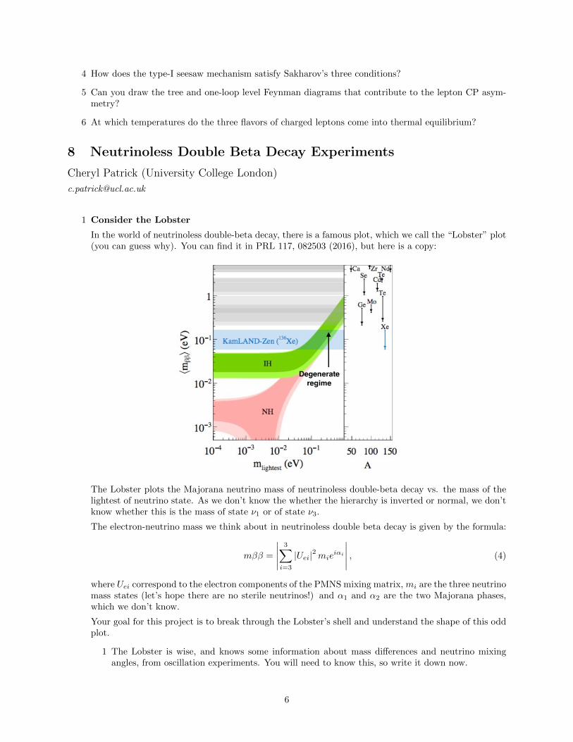
In the world of neutrinoless double-beta decay, there is a famous plot, which we call the “Lobster” plot(you can guess why). You can find it in PRL 117, 082503 (2016), but here is a copy:

The Lobster plots the Majorana neutrino mass of neutrinoless double-beta decay vs. the mass of thelightest of neutrino state. As we don’t know the whether the hierarchy is inverted or normal, we don’tknow whether this is the mass of state ν1 or of state ν3.

The electron-neutrino mass we think about in neutrinoless double beta decay is given by the formula:

mββ =

∣∣∣∣∣3∑

i=3

|Uei|2mieiαi

∣∣∣∣∣ , (4)

where Uei correspond to the electron components of the PMNS mixing matrix, mi are the three neutrinomass states (let’s hope there are no sterile neutrinos!) and α1 and α2 are the two Majorana phases,which we don’t know.

Your goal for this project is to break through the Lobster’s shell and understand the shape of this oddplot.

1 The Lobster is wise, and knows some information about mass differences and neutrino mixingangles, from oscillation experiments. You will need to know this, so write it down now.

6

2 The double-beta mass is a kind of effective electron neutrino mass. Experiments like KATRIN,which look at the beta decay spectrum end-point, also measure an electron (anti)neutrino mass,which is also a combination of values from the PMNS matrix. Find out the expression for thismass mβ.

a Does it depend on CP violating phases or Majorana phases? If it does, continue this questionassuming that they are all zero.

b Is it the same as mββ? If not, how does it differ?

c Is it possible for mβ to be zero, given the constraints we have from oscillation experiments?Using just the oscillation information, can you put any (upper or lower) limits on mβ?

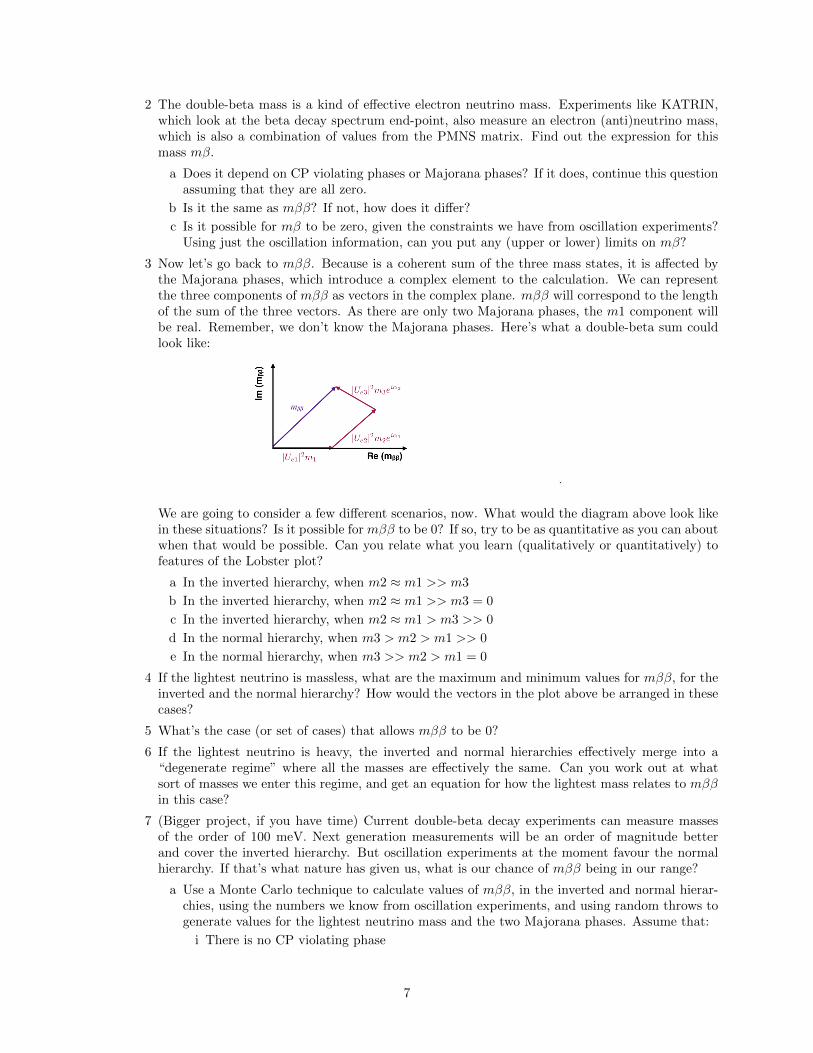
3 Now let’s go back to mββ. Because is a coherent sum of the three mass states, it is affected bythe Majorana phases, which introduce a complex element to the calculation. We can representthe three components of mββ as vectors in the complex plane. mββ will correspond to the lengthof the sum of the three vectors. As there are only two Majorana phases, the m1 component willbe real. Remember, we don’t know the Majorana phases. Here’s what a double-beta sum couldlook like:

We are going to consider a few different scenarios, now. What would the diagram above look likein these situations? Is it possible for mββ to be 0? If so, try to be as quantitative as you can aboutwhen that would be possible. Can you relate what you learn (qualitatively or quantitatively) tofeatures of the Lobster plot?

a In the inverted hierarchy, when m2 ≈ m1 >> m3

b In the inverted hierarchy, when m2 ≈ m1 >> m3 = 0

c In the inverted hierarchy, when m2 ≈ m1 > m3 >> 0

d In the normal hierarchy, when m3 > m2 > m1 >> 0

e In the normal hierarchy, when m3 >> m2 > m1 = 0

4 If the lightest neutrino is massless, what are the maximum and minimum values for mββ, for theinverted and the normal hierarchy? How would the vectors in the plot above be arranged in thesecases?

5 What’s the case (or set of cases) that allows mββ to be 0?

6 If the lightest neutrino is heavy, the inverted and normal hierarchies effectively merge into a“degenerate regime” where all the masses are effectively the same. Can you work out at whatsort of masses we enter this regime, and get an equation for how the lightest mass relates to mββin this case?

7 (Bigger project, if you have time) Current double-beta decay experiments can measure massesof the order of 100 meV. Next generation measurements will be an order of magnitude betterand cover the inverted hierarchy. But oscillation experiments at the moment favour the normalhierarchy. If that’s what nature has given us, what is our chance of mββ being in our range?

a Use a Monte Carlo technique to calculate values of mββ, in the inverted and normal hierar-chies, using the numbers we know from oscillation experiments, and using random throws togenerate values for the lightest neutrino mass and the two Majorana phases. Assume that:

i There is no CP violating phase

7

ii The probability for the log of the lightest neutrino mass (in eV) is evenly distributedbetween 0 and ∼ 4.

iii The probabilities for the two Majorana phases are evenly distributed between 0 and 2π.

b Plot the values you get for the randomly-chosen lightest neutrino mass and your calculatedmββ on 2d histograms (one each for normal and inverted hierarachy). You made your ownlobster plots! What did you learn?

c Now you’re at it, why not try calculating mβ as well and plot mβ vs mββ?

2 Your 0νββ future

It’s 2030, England has just won the World Cup, and you’ve just landed a top job at Fermilab! Whata great year! Even more exciting, LEGEND http://legend-exp.org and NEXO https://nexo.

llnl.gov experiments have just announced that they have observed neutrinoless double-beta decay.LEGEND measured a half-life of 5× 1027 years for their isotope, while NEXO measured a half-life of7.5× 1027 years. In each case, they have a 20% uncertainty on their measurement.

– What neutrino mass limits do these correspond to? (Hint: arXiv:1610.06548 [nucl-th])

– Do you think the two measurements are compatible? (Think about the different isotopes and howthey behave differently).

– What half-life would you expect SNO+ https://www.snolab.ca/science/experiments/snoplus tomeasure?

– Do they tell us anything else about the nature of the neutrino?

Now that neutrinoless double beta decay is in the news, Fermilab wants you, their hottest new scientist,to design a new experiment to learn more about it. There’s lots of cash available, and you have accessto the resources of the lab and the current far detector locations of the Fermilab oscillation experiments.Propose your new design! Some things to think about:

– What do you aim to learn with your new experiment? (Think about nuclear physics, masshierarchy, double-beta decay mechanisms).

– What isotope(s) would you use? How much will you need, and what do you estimate it will cost?Why is this a good choice? Do you save on other detector components? Can your detector beused for anything else as well?

– What detector technology will you use? Feel free to be creative and steal the best ideas fromcurrent detectors like KamLAND Zen, GERDA, SNO+, SuperNEMO, and CUORE.

9 Lepton-Nucleus Cross Section Theory

Noemi Rocco (Argonne National Lab & Fermilab)

c.patrick@ucl.ac.uk

1. Consider the charge-current scattering process: ν−` + n→ `− + p where ` = e, µ, τ .

• What is the minimum value of the energy transfer ω for which the reaction can take place?

• Consider the case in which ` = µ− and the elastic scattering happens on a neutron at rest, i.e.the neutron quadri-momentum is given by (mn, 0) and the proton (mp + ω,q). Show that thereconstructed neutrino energy reads

Eν =m2p −m2

n −m2µ + 2mnEµ

2(mn − Eµ + pµ cos θµ), (5)

where θµ is the muon angle relative to the neutrino beam.

8

• Write down the analogous expression for a moving neutron in the initial state, i.e. (En,pn). Toderive the neutrino energy expression, define the angle between the neutron and the neutrinobeam momentum as cos θn = (kν · pn)/(|kν ||pn|).

2. The most general expression for the hadronic tensor is constructed out of gµν and the independentmoment of the initial nucleon p and the momentum transfer q, yielding

Wµν = −W1gµν +

W2

m2N

pµpν + iεµναβW3

2m2N

pαqβ +W4

m2N

qµqν +W5

m2N

(pµqν + pνqµ) (6)

where Wi are called structure functions and mN is the nucleon mass.

• In the electromagnetic case parity-violating effects are NOT present. The hadronic electromag-netic current matrix elements are polar-vectors and so the tensor must have specific propertiesunder spatial inversion. In particular, in this case W3 = 0. The current conservation condition atthe hadronic vertex requires

qνWµν = qµW

µν = 0 (7)

As a result of this relation, verify that only two structure functions are independent and thehadronic electromagnetic tensor reads

Wµν = W1

(gµν +

qµqν

q2

)+W2

m2N

(pµ − p · q

q2qµ

)(pν − p · q

q2qν

)(8)

• For the scattering process ν−µ + n → µ− + p, the double-differential cross section is proportionalto

d2σ

dEµdΩµ∝ LµνWµν . (9)

The contraction between the leptonic and hadronic tensor can be rewritten as

LµνWµν =

16

m2N

5∑

i=1

LiWi (10)

where the W i are the structure functions reported above and Li are leptonic factors, you can findthe explicit expression in in Nucl. Phys. A 789, 379 (2007) or try to compute them. How wouldthis generic expression change for the νµ scattering process?

10 Origin and Nature of Neutrino Mass

Goran Senjanovic (ICTP)

goran@gssi.infn.it

These problems cover the essence of my course. The first problem is simply a summary of Dirac andMajorana spinors in the two-component form. This material is a pre-requisite, so I strongly advice you tofind some time to go through it in case you are not familiar with the math and physics of Dirac and Majoranamass. The other problems cover the lectures’ material and doing them would help tremendously understandthe subtleties of the physics involved. I wish to warn you that there could be misprints or even an occasionalerror, so please contact me if you have any comments or questions regarding this material.

Problem 1

A four-component Dirac spinor transforms under the Lorentz group as

Ψ→ SΨ, S ≡ eiθµνΣµν , (11)

9

with

Σµν ≡ 1

4i[γµ, γν ], γµ, γν = 2gµν , (12)

with the explicit form for Dirac matrices in my conventions

γ0 =

(0 II 0

), γi =

(0 σi

−σi 0

)

1. Show that the Σµν satisfy the Lorentz algebra. You can do in a generic manner, or even better, byseparating the rotations and boosts, and then check the usual relations among rotations and boosts.

2. Introduce Left and Right chiral spinors

ΨL,R ≡1± γ5

2Ψ ≡ L (R) Ψ (13)

γ5 = −i γ0 γ1 γ2 γ3

or

γ5 =

(I 00 −I

)

Using Eq. (1), show that

uL(R) → ei~σ/2(~θ±i~φ)uL(R) (14)

where

ΨL =

(uL0

), ΨR =

(0uR

)

What does ~θ represent? And ~φ?

3. Take a boost in the z-direction and find an expression for ~φ.

4. Define charge-conjugation transformation

Ψc ≡ CΨT

(15)

withCT γµC = −γTµ , CT = C† = C−1 = −C

An explicit choice: C = iγ2γ0.

Show thatΨc → SΨc (16)

when Ψ→ SΨ. In other words, Ψc transforms the same way as Ψ, i.e. it is also a proper spinor.

5. Take

Ψ = ΨL =

(uL0

)

Compute Ψc. What is its chirality ?

6. What happens to uL and uR under parity? By definition, under parity transformation

Ψ→ γ0Ψ

in order to have the four vector ΨγµΨ behave correctly (three-vector and a scalar).

10

Now take a four-component Majorana spinor ΨM , defined by

ΨM = ΨcM

1. Show that ΨM can be written as

ΨM =

(uL

−iσ2u∗L

)

or equivalently

ΨM = ΨL + C ΨLT. (17)

2. Take the free Majorana Lagrangian

L = iΨMγµ∂µΨM −mΨMΨM (18)

Show that this is equivalent to

L = iu†Lσµ∂µuL −

1

2m(uTL iσ2uL + h.c.

)(19)

where σµ = (1;−σi) (and σµ = (1;σi), which enters for RH spinors).

3. Show the following vector current vanishes

ΨMγµΨM

Can you explain why?

Hint: can there be invariance under ΨM → e−iαΨM?

11

Problem 2

Multi-generation see-saw mechanism. This exercise serves to understand the properties of Majoranaspinors and the seesaw mechanism of neutrino mass - an important aspect of the course.

We introduce a gauge singlet fermion, the so-called RH neutrino νR, per generation and write down themost general Yukawa interaction for n generations

LY = νR Φ† YD `L + νTR CM†N

2νR + h.c. (20)

where we use a compact notation for the following vectors in the generation space

νR =

ν1

.

.νn

R

, `L =

`1..`n

L

(21)

with the usual notation for leptonic and Higgs doublets

`iL =

(νiei

)

L

, Φ = iσ2Φ∗ (22)

Thus, in (20), YD and MN are n× n matrices in the generations space.

• Show that MN is a symmetric matrix. This is a general property of Majorana mass matrices of thesame species of particles.

• Show that (20) is invariant under the SM SU(2)× U(1) gauge symmetry.

• IntroducingNiL ≡ CνTiR (23)

show that (20) can be written as

LY = NTL C ΦT (−iσ2)YD `L + NT

L CMN

2NL + h.c. (24)

• From the usual form for the Higgs doublet in the unitary gauge

Φ =1√2

(0

h+ v

)

show

Lmass = NTL CMDνL + NT

L CMN

2NL + h.c. (25)

where

MD =YD v√

2(26)

• Show next

Lmass =1

2

[νTL M

TD C NL + NT

L MD C νL + NTL MN C NL

]+ h.c.. (27)

In other words, one has a mass matrix (up to a factor 1/2) between νL and NL

MνN =

(0 MT

D

MD MN

)(28)

12

• Assume MN MD and show that (28) can be put in block-diagonal form as

DνN =

(Mν 00 MN

)(29)

by a unitary transformationUT MνN U = DνN

where

U =

(1 Θ†

−Θ 1

)(30)

andMν = −MT

DM−1N MD (31)

with Θ = M−1N MD, and where only terms up to order Θ2 are considered.

• Next diagonalize symmetric matrices Mν and MN by unitary matrices VL and VR

Mν = V ∗LmνV†L (32)

and similarly for MN . The convention above corresponds to VL being the leptonic mixing matrix (thePMNS matrix) in the basis of diagonal charged leptons

g√2νLγ

µVLeLW+µ (33)

where ν and e stand for all the neutrinos and charged leptons respectively.

Recall that one can always fix such a basis since mixings depend on the relative rotations betweenneutrinos and charged leptons - just as in the case of up and down quarks discussed in the class.

• Once obtained, the physical states (eigenstates of mass matrices) can be cast in the 4-dimensionalMajorana form as in the problem 1. Do that and show that the factor 1/2 in (27) is not physical.

• Once neutrinos are massive, there will be flavor mixings in the leptonic sector. As usual, there will bein general CP phases.

If neutrinos are Majorana particles, is the number of phases the same as in the Dirac case (i.e. thequark case)? More precisely, we speak here of physical phases that cannot be rotated away by phaseredefinitions. In particular, does one need three generations in order to have CP violation? Computethe number of physical phases for n generations.

13

Problem 3

a. Let us imagine that neutrino is a Majorana particle, i.e. ν ≡ νL + C νLT . This happens naturally

in the seesaw mechanism of the above problem, when there exist a heavy neutral Majorana lepton

N ≡ NL + C NLT

, with a mass mN . Neutrino gets a mass through the mixing with N which thenleads to N having weak interaction

L =g√2θW+

µ NγµLe+ h.c., (34)

where L is the usual chiral projector L = (1 + γ5)/2. In the above formula θ = mD/mN =√mν/mN

is the mixing between ν and N , and mD = yDv is the Dirac mass term between ν and N . In the usualnotation, v is the vacuum expectation value v of the Higgs field and yD is what we call the neutrinoDirac Yukawa coupling defined through the interaction

yDNTLCνL(h+ v) + h.c. (35)

i. Compute the decay rate N →W+ + e. Neglect the electron mass.

ii. What is the result in the limit of the vanishing W mass? Does the result depend on how you takethe limit, i.e. whether the gauge coupling g goes to zero or the vacuum expectation value v? Can youexplain what is going on in both cases? This is the test of your knowledge of the Yang-Mills theory.

iii. Is there another decay channel? Recall that N is Majorana particle, or better half-particle and half-antiparticle.

iv. Compute the lifetime of N .

b. Let us imagine that there is a another heavy W ′ boson with the following interaction

L′ =g′√

2W ′+µ [NγµL(R)e+ uγµL(R)d] + h.c. (36)

and assume MW ′ > mN . The notation says that the W ′ has either purely LH or RH couplings.

i. Compute the three body decay rate N → e+ u+ d. You can set all masses to zero, except for mN . Ifyou find it it too long or too hard, use the analogy with the muon 3-body decay, so that you can dothe rest below.

ii. Is this the only channel?

iii. Does the decay rate depend whether the coupling is L or R?

iv. Compute the lifetime of N in this case.

v. Take g′ = g, mν = 0.1eV, mN = 240GeV, mW ′ = 4.8TeV and compare the values for the 2 and3-body decay rates that you computed. Which is bigger? This situation is a realistic possibility forthe so-called LR symmetric theory that predicted originally massive neutrinos and led to the seesawmechanism.

14

Problem 4

Left-Right Symmetry and Neutrino mass. As discussed in the lectures, the LR symmetric extensionof the SM, put forward in order to understand parity violation in weak interactions, led originally to theexistence of the RH neutrino and neutrino mass. Moreover, it provides a natural framework for the seesawmechanism.

Take a LR symmetric theory based on the gauge group

GLR = SU(2)L × SU(2)R × U(1)B−L

with fermions transforming as

`L =

(νe

)

L

;

(νe

)

R

= `R

qL =

(ud

)

L

;

(ud

)

R

= qR (37)

so that the covariant derivative is

Dµ = ∂µ − ig ~TL · ~AµL − ig ~TR · ~AµR − ig′(B − L)

2Bµ (38)

where

(B − L)` = −`, (B − L)q =1

3q (39)

Assume the existence of Higgs triplets ∆L and ∆R in the adjoint representations of SU(2)L and SU(2)Rrespectively, with

∆L,R → UL,R ∆L,R U†L,R (40)

where`L,R → UL,R `L,R, qL,R → UL,R qL,R (41)

• Show that the Yukawa interaction

L∆ = y∆

(`TL C iσ2 ∆L `L + `TR C iσ2 ∆R `R + h.c.

)(42)

is invariant under GLR. This of course implies the B − L gauge numbers of the triplets to be

(B − L)∆L,R = 2∆L,R (43)

• Take the following potential

V = −µ2(

Tr∆†L∆L + Tr∆†R∆R

)+λ

4

[(Tr∆†L∆L)2 + (Tr∆†R∆R)2

]

+λ′

2Tr∆†L∆L Tr∆†R∆R (44)

– Find under which conditions one gets a minimum

〈∆L〉 = 0, 〈∆R〉 6= 0 (45)

– Show that

〈∆R〉 =

(0 0vR 0

)(46)

preserves the SM gauge symmetry SU(2)L × U(1)Y , with

Y

2≡ T3R +

B − L2

(47)

and

Q = T3L + T3R +B − L

2(48)

15

• Find the masses of the heavy gauge fields W±R and ZR, and determine ZR as a function of the originalfields in (38)

• Show that (42) produces the Majorana mass of the RH neutrino.

• Defining as in the seesaw picture (Problem 3) NiL ≡ CνTiR, show that LR symmetry dictates

MN = VRmNVTR (49)

in analogy with the light neutrino mass matrix

Mν = V ∗LmNV†L . (50)

In other words, this guarantees that the LH and RH PMNS mixing matrices are given symmetrically.Show that the above equations correspond to the gauge interactions with the LH and RH W bosons

Lgauge =g√2

(νLγµV†LeLW

µL + νRγµV

†R eRW

µR) (51)

The LH mixing matrix VL is measured by neutrino oscillation experiments, neutrinoless double betadecay and other low energy experiments, whereas its RH analog VR would be measured principally athadron colliders such as the LHC.

• Let us take the LR symmetry a step further, and use it to compute the neutrino Dirac mass matrix.Take LR to be (generalised) charge conjugation as discussed in the course

ψL → CψTR (52)

in which case it is to see that Yukawa couplings must be symmetric, and similarly the fermion massmatrices, in particular the neutrino Dirac mass matrix

MTD = MD. (53)

Use this to disentangle the seesaw

MD = iMN

√M−1N Mν . (54)

Next, for the sake of illustration assume VR = V ∗L which corresponds to the unrealistic unbroken LRsituation, and show that MD takes a simple form

MD = V ∗L√mNmνV

†L (55)

where mN and mν are diagonal heavy and light neutrino mass matrices.

• In the problem 2, one shows that the ν − N mixing matrix is given by Θ = M−1N Mν , so that for the

above case of LR symmetry being charge conjugation, one obtains

Θ = i√M−1N Mν . (56)

Knowing Θ determines decay rates of N to charged leptons and W, Ni → `jW+ just as the knowledge

of charged fermion masses determines Higgs decays h→ ff in the SM. It shows that the LR symmetrictheory does for neutrino mass what the SM does for charged fermions - allows to probe their Higgsmass origin. In the case of neutrinos, their Majorana nature requires the knowledge of both Mν andMN in analogy of mf in the case of quarks and charged leptons.

Show that for VR = V ∗L , this can be written as

Θ = iVL

√m−1N mνV

∗L (57)

Use this expression to show that the decay rate of Ni into a `j charged lepton is proportional to

Γ(Ni →W`j) ∝ |Vji|2mνi

m2Ni

M2W

. (58)

Determine the constant of proportionality using the result of problem 2.

16

Problem 5

Effective d=5 interaction for neutrino mass. Imagine that we add no new particles to the SM, inwhich case neutrino is massless at the renormalizable d=4 level.

1. Now, add a dimension five operator(lTLσ2Φ)C(ΦTσ2lL)

M(59)

where lL is the SM lepton doublet and Φ is the usual Higgs scalar doublet.

2. Show that the above interaction is allowed by the SM gauge symmetry.

3. What happens when the Higgs gets a vev? Compare with the see-saw formula.

4. Show that there are only three ways of writing the above operator. Then show that they are allequivalent.

5. Go to the physical unitary gauge and determine the leading Higgs boson-neutrino Yukawa interactionShow that it is proportional to neutrino mass as expected from the Higgs mechanism.

11 Neutrino Astronomy

Francis Halzen (University of Wisconsin)

francis.halzen@icecube.wisc.edu

Cosmic neutrinos are produced in Galactic and extragalactic cosmic accelerators that accelerate protons(nuclei) to more than a hundred million TeV. Cosmic neutrinos are produced in cosmic beam dumps wherethe target is provided by the radiation fields (yes, photons are the target) and dust or molecular cloudssurrounding the accelerator. Given the large luminosity (and not just the high energy) of the acceleratorsthat we observe, it is believed that the power is provided by the large gravitational energy associated withthe collapse of stars, or with the particle flows into supermassive black holes residing at the centers of activegalaxies (black holes feeding on their own galaxy). Shock waves are believed to be the mechanism by which1 10

Research the principle of first and second order Fermi acceleration. If you find a really great explanationon the web or in a text book, let me know. I recommend the early references by E. Fermi.

1. Summarize the essential concept of shock acceleration in less than 3 ppt slides.2. Make a plot of the velocity of the particles moving across the shock in 4 frames, the lab frame, the

frame where the shock is at rest, the frame where upstream particles are at rest and the frame where thedownstream particles are at rest. (Note the gain in energy when the particle crosses the shock in eitherdirection).

3. Do the problem set #4 in the problems sets attached below.

17

Problems — Neutrino Astronomy The problem sets accompanying the neutrino astronomy presentation are somewhat different. They provide a set of exercises (with solutions) to refresh concepts that may be unfamiliar to particle physicists and are relevant to understanding the talk. You may also want to consult Wikipedia if you are not familiar with some of the concepts. The 4 sets cover:

n Relativistic kinematics applied to cosmic rays, particle decays and interactions. n Particle and photon fluxes from astronomical objects. n Interaction lengths, superluminal motion and luminosity. n Shock waves and Fermi acceleration.

Francis Halzen

Series 1 – Relativistic kinematics, Particle Decays

July 29, 2019

Notation: a vector v has a module v and a versor v

Ex. 1 — Relativistic kinematicsAtmospheric muons are created at an altitude of about 10 km, with velocity β = 0.999.

1. — Calculate the average distance that they travel before to decay. Do they reach theground?

2. — Imagine to be a muon: do you reach the ground?3. — Do pions generated with the same velocity reach the ground?

Answer (Ex. 1) —

1. — In the reference system of the Earth, the average distance covered by the muons isgiven by d = γβcτ0, where γ = 1/

√(1− β2) = 22.37, cτ0 = 658.7 m :

d = 22.37 · 0.999 · 658.7 m = 14.7 km. (1)

So muons can reach the ground.2. — In the reference system of the muon obiouvsly its mean lifetime is invariant, τ0, and

the distance that it can cover in this case is:

d = 0.999 · 658.7 m = 658.0 m. (2)

The reason why it can reach the ground is that the distance to be covered is shortened,h = 10000/γ ' 447.03 m.

3. — Charged pions have a much shorter mean lifetime, cτ0 = 7.8 m, so they can cover amuch shorter length (assuming for simplicity the same γ):

d = 22.37 · 0.999 · 7.8 m = 174.3 m (3)

so they can not reach the ground.

Ex. 2 — Relativistic kinematicsConsider a neutron produced by an astrophysical phenomenon. The energy of the neutron isequivalent to the energy of a proton accelerated in a fixed gas-target experiment at a center-of-mass energy of 14 TeV. Consider the target made of hydrogen.

1. — If the neutron would be produced by a cosmic source, what is the order of its energy?

1

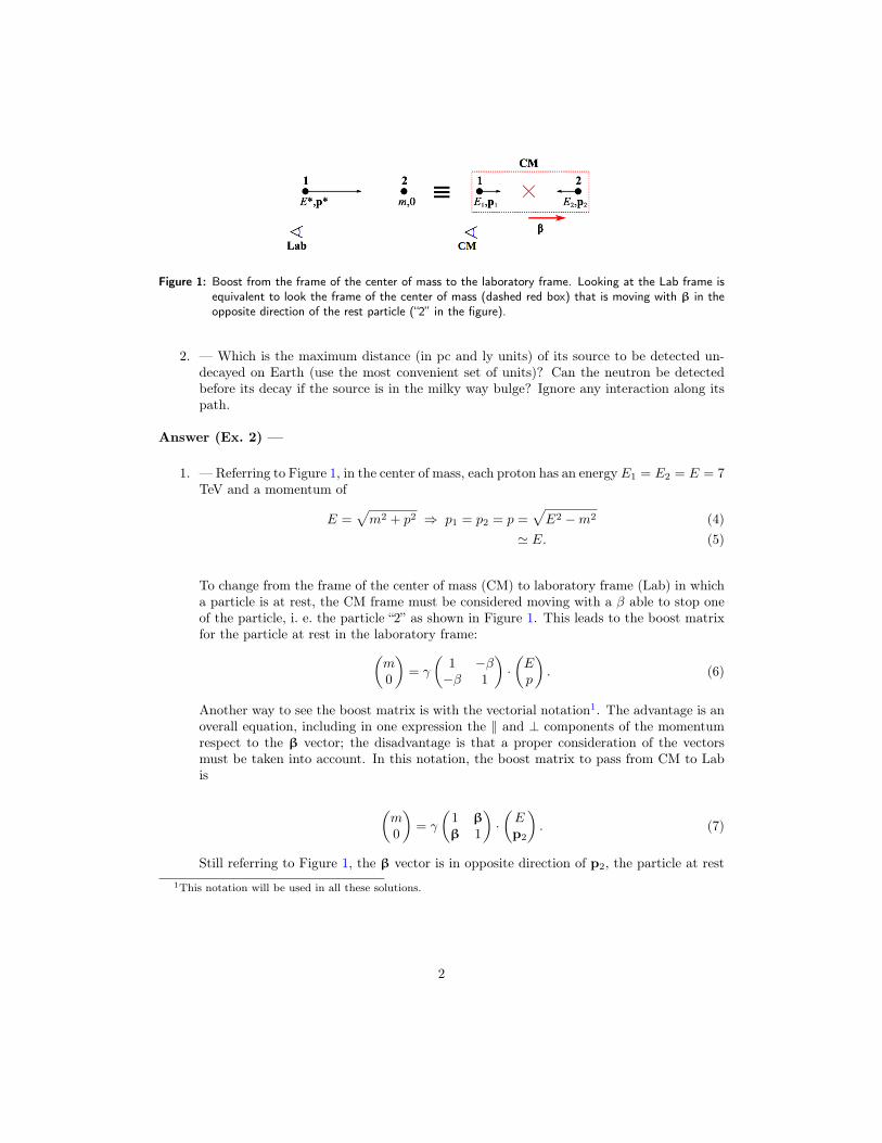
Figure 1: Boost from the frame of the center of mass to the laboratory frame. Looking at the Lab frame isequivalent to look the frame of the center of mass (dashed red box) that is moving with β in theopposite direction of the rest particle (“2” in the figure).

2. — Which is the maximum distance (in pc and ly units) of its source to be detected un-decayed on Earth (use the most convenient set of units)? Can the neutron be detectedbefore its decay if the source is in the milky way bulge? Ignore any interaction along itspath.

Answer (Ex. 2) —

1. — Referring to Figure 1, in the center of mass, each proton has an energy E1 = E2 = E = 7TeV and a momentum of

E =√m2 + p2 ⇒ p1 = p2 = p =

√E2 −m2 (4)

' E. (5)

To change from the frame of the center of mass (CM) to laboratory frame (Lab) in whicha particle is at rest, the CM frame must be considered moving with a β able to stop oneof the particle, i. e. the particle “2” as shown in Figure 1. This leads to the boost matrixfor the particle at rest in the laboratory frame:

(m0

)= γ

(1 −β−β 1

)·(Ep

). (6)

Another way to see the boost matrix is with the vectorial notation1. The advantage is anoverall equation, including in one expression the ‖ and ⊥ components of the momentumrespect to the β vector; the disadvantage is that a proper consideration of the vectorsmust be taken into account. In this notation, the boost matrix to pass from CM to Labis

(m0

)= γ

(1 ββ 1

)·(Ep2

). (7)

Still referring to Figure 1, the β vector is in opposite direction of p2, the particle at rest1This notation will be used in all these solutions.

2

in the lab frame; that yields, using Equation (4),

m = γ(E − β

√E2 −m2

)= γE

1− β

√

1− m2

E2

, (8)

0 = γ(βE −

√E2 −m2

)⇒ β =

√

1− m2

E2' 1. (9)

From Equation (9), the Equation (8) gives the γ factor:

m = γE(1− β2

)=E

γ⇒ γ =

E

m≈ 7000. (10)

If the same boost is applied to the particle “1”, which has p1 in the same direction of β,and the approximations in Equations (5) and (9) are used, the estimation of the particleenergy (and momentum) is

(E∗

p∗

)= γ

(1 ββ 1

)·(Ep1

)' γ

(1 11 1

)·(EE

)⇒ E∗ = 2γE ∼ 1017 eV, (11)

where the index ∗ denotes the laboratory frame.2. — The maximum distance of its source is:

l∗ = τ∗c = γτcβ ' 2.9 · 1016 km (12)

⇒ l∗ ' 2.9 · 103 ly (13)

⇒ l∗ ' 9.25 · 102 pc, (14)

where γ = En/mn = 1.11 · 108 was used. From these results, it is quite obvious that anyneutron produced in the milky way bulge cannot reach un-decayed the earth surface.

Ex. 3 — Relativistic kinematicsA proton travelling in the space interacts with the cosmic radiation background at 3K.

1. — Calculate the energy threshold of the proton to allow the reactions p+ γ → p+π0 andp+ γ → p+ e+ + e− in case of frontal collisions.

2. — If the π photo-production cross-section is 100 µbarn and is constant, calculate theproton mean free path as a function of the energy. Remember that the mean free path isgiven by λ = 1/ρσ and ρ = 0.24(kT/c)3 for a black body.

Answer (Ex. 3) —

1. — Let’s do the calculations for the process p + γ → p + π0. The invariant mass of thesystem is conserved:

(pp + pγ)2 = (p′p + p′π0)2,

where p is the 4-momentum p = (E, ~p).

For the left hand term of the equation:

3

(pp + pγ)2 = p2

p + p2γ + 2pppγ =

= E2p − | ~pp|2 + E2

γ − | ~pγ |2 + 2(EpEγ − | ~pp|| ~pγ |cosθ) =

= m2p +m2

γ + 2EpEγ − 2| ~pp|| ~pγ |cosθ,

where θ is the angle between the proton and the pion.Hence the full equation becomes:

m2p + 2EpEγ − 2pppγcosθ =m

2p +m2

π0 + 2E′pE′π0 − 2p′pp

′πcosθ

At the threshold, p′π = p′p = 0.Under the hypothesis of high energies, Ep mp:

2EpEγ(1− cosθ) = 2E′pE′π0 +m2

π0 = m2π0 + 2mpmπ0

Considering that:

mp = 938.27 MeV ≈ 103 MeVmπ0 = 134.9766 MeV ≈ 102 MeV2mpmπ0 ≈ 2 · 105 MeVm2π0 ≈ 104 MeV → negligible wrt 2mpmπ0

Considering only frontal collisions:

4EpEγ = 2mpmπ0

Ep,threshold =mpmπ0

2Eγ' 5 · 1020 eV,

where Eγ ∼ kT = 25 · 10−5 eV.

When the scattering is more complicated, as in the case p+ γ → p+ e+ + e−:

(pp + pγ)2 = (p′p + p′e+ + p′e−)

2,

m2p + 2EpEγ − 2| ~pp|| ~pγ |cosθ = m2

p +m2e +m2

e + 2p′pp′e+ + 2p′pp

′−e + 2p′e−p′e+

m2p + 2EpEγ − 2| ~pp|| ~pγ |cosθ = 4mpme +m

2p + 4m2

e

E =(mpme+m

2e)

Eγ' 2 · 1018 eV.

2. — σ(p+ γ → p+ π) = 100 µbarn = 10−32m2

λ = 1/ρσ, with ρ = 0.24(kT/c)3 = 5 · 1017m−3 → λ = 2 · 105 m.

Ex. 4 — Particles decayIn nature the stable particles are few. Most of them are unstable and they decay. In this exercisethe decay π+ → µ+ + νµ (a mesonic decay) is considered.

1. — Calculate the momentum of µ+ and νµ in the rest frame, assuming the neutrino asmassless.

4

2. — The neutrino is not massless but it has a small mass, so far measured only as upperlimit. Measuring the muon momentum, the mass of the νµ can be constrained. Howmuch must the precision on the measurement of the muon momentum be to determinethe current upper limit of the νµ mass (190 keV).

3. — Assume that the π+ has an initial momentum of 500 MeV (in natural units). If thismomentum is perpendicular to the direction along which the decay in the rest frame ofthe pion occurs, how much is the (massless) neutrino energy and how much is the anglebetween µ+ and νµ?

Answer (Ex. 4) —

1. — “Neutrino massless” means Eν = pν . Therefore the energy and momentum conservationyield

mπ =√p2µ +m2

µ + Eν , (15)

0 = pµ + pν . (16)

Through Equation (16), p2µ = E2

ν . Isolating the root square in Equation (15) and squaringgives

(mπ − Eν)2 = E2ν +m2

µ

⇒ m2π +E

2ν − 2mπEν =E

2ν +m2

µ,

therefore, with mπ = 139.6 MeV and mµ = 105.7 MeV,

⇒ Eν = pν = pµ =m2π −m2

µ

2mπ= 29.7839183 ' 29.8 MeV (in natural units). (17)

2. — With mν 6= 0, the Equation (15) becomes

mπ =√p2µ +m2

µ +√p2ν +m2

ν , (18)

that leads to pµ:

(mπ −

√p2µ +m2

µ

)2

=(√

p2µ +m2

ν

)2

⇒ m2π +p

2µ +m2

µ − 2mπ

√p2µ +m2

µ = p2µ +m2

ν

⇒(2mπ

√p2µ +m2

µ

)2

=(m2π +m2

µ −m2ν

)2

⇒ 4m2π

(p2µ +m2

µ

)=(m2π +m2

µ −m2ν

)2

⇒ p2µ =

(m2π +m2

µ −m2ν

)2

4m2π

−m2µ. (19)

In case of mν = 0, the Equation (19) gives the Equation (17) (pµ|mν=0 = 29.7839183MeV). In case of mν = 0.19 MeV,

pµ|mν=0.19 = 29.7834416 MeV (in natural units). (20)

5

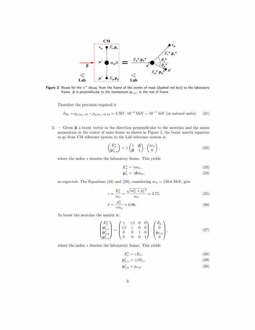
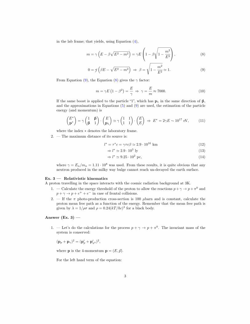
Figure 2: Boost for the π+ decay, from the frame of the center of mass (dashed red box) to the laboratoryframe. β is perpendicular to the momentum pν(µ) in the rest of frame.

Therefore the precision required is

δpµ = pµ|mν=0 − pµ|mν=0.19 ' 4.767 · 10−4 MeV ∼ 10−1 keV (in natural units). (21)

3. — Given β a boost vector in the direction perpendicular to the neutrino and the muonmomentum in the center of mass frame as shown in Figure 2, the boost matrix equationto go from CM reference system to the Lab reference system is:

(E∗πp∗π,x

)= γ

(1 ββ 1

)·(mπ

0

), (22)

where the index ∗ denotes the laboratory frame. This yields

E∗π = γmπ, (23)p∗π = γβmπ, (24)

as expected. The Equations (23) and (29), considering mπ = 139.6 MeV, give

γ =E∗πmπ

=

√m2π + p∗π

2

mπ' 3.72, (25)

β =p∗πγmπ

' 0.96. (26)

To boost the neutrino the matrix is:

E∗πp∗ν,xp∗ν,yp∗ν,z

=

γ γβ 0 0γβ γ 0 00 0 1 00 0 0 1

·

Eν0

pν,y0

, (27)

where the index ∗ denotes the laboratory frame. This yields

E∗ν = γEν , (28)p∗ν,x = γβEν , (29)

p∗ν,y = pν,y. (30)

6

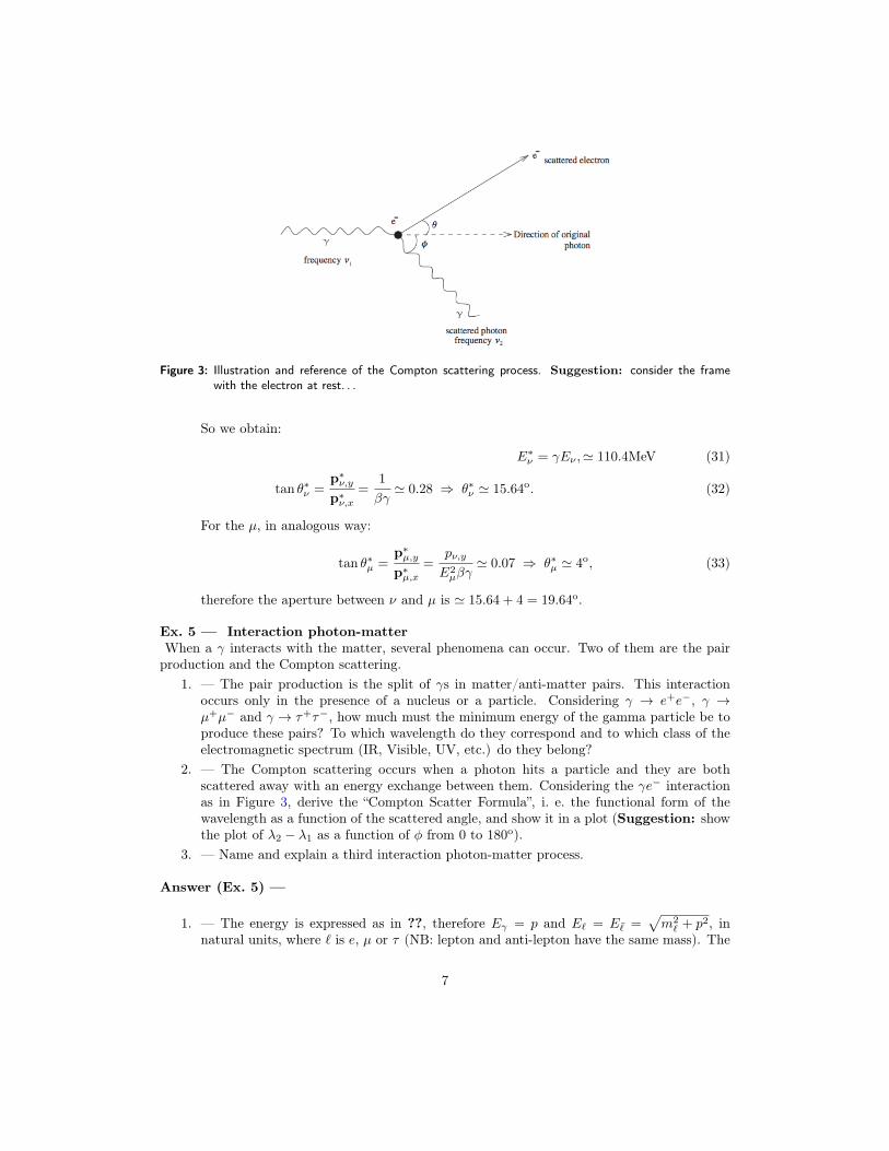
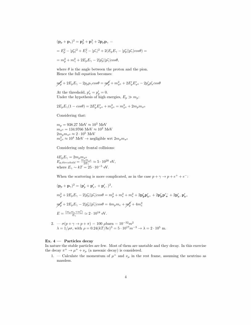
Figure 3: Illustration and reference of the Compton scattering process. Suggestion: consider the framewith the electron at rest. . .

So we obtain:

E∗ν = γEν ,' 110.4MeV (31)

tan θ∗ν =p∗ν,yp∗ν,x

=1

βγ' 0.28 ⇒ θ∗ν ' 15.64o. (32)

For the µ, in analogous way:

tan θ∗µ =p∗µ,yp∗µ,x

=pν,y

E2µβγ

' 0.07 ⇒ θ∗µ ' 4o, (33)

therefore the aperture between ν and µ is ' 15.64 + 4 = 19.64o.

Ex. 5 — Interaction photon-matterWhen a γ interacts with the matter, several phenomena can occur. Two of them are the pairproduction and the Compton scattering.

1. — The pair production is the split of γs in matter/anti-matter pairs. This interactionoccurs only in the presence of a nucleus or a particle. Considering γ → e+e−, γ →µ+µ− and γ → τ+τ−, how much must the minimum energy of the gamma particle be toproduce these pairs? To which wavelength do they correspond and to which class of theelectromagnetic spectrum (IR, Visible, UV, etc.) do they belong?

2. — The Compton scattering occurs when a photon hits a particle and they are bothscattered away with an energy exchange between them. Considering the γe− interactionas in Figure 3, derive the “Compton Scatter Formula”, i. e. the functional form of thewavelength as a function of the scattered angle, and show it in a plot (Suggestion: showthe plot of λ2 − λ1 as a function of φ from 0 to 180o).

3. — Name and explain a third interaction photon-matter process.

Answer (Ex. 5) —

1. — The energy is expressed as in ??, therefore Eγ = p and E` = E¯ =√m2` + p2, in

natural units, where ` is e, µ or τ (NB: lepton and anti-lepton have the same mass). The

7

minimum case is when p = 0; hence, for the energy conservation,

Eγ = E` + E¯ = m` +m¯ = 2m`. (34)

Therefore

γ → e+e− : Eγ = 2 · 0.511 ' 1.022 MeV, (35)

γ → µ+µ− : Eγ = 2 · 106 ' 212 MeV, (36)

γ → τ+τ− : Eγ = 2 · 1.777 ' 3.554 GeV (37)

and, remembering that we can divide a length x by c ' 197 MeV·fm, to convert awavelength from natural units to SI,

λe+e− =2π

1.022= 6.14 MeV−1 ⇒ 1.26 pm, (38)

λµ+µ− =2π

212= 0.03 MeV−1 ⇒ 5.91 fm, (39)

λτ+τ− =2π

3.554= 1.77 GeV−1 ⇒ 0.35 fm. (40)

All of them are γ-rays and only the electron-positron production is close to the X-rays.2. — Labelling the initial and final states of the photon with subscripts 1 and 2 respectively

as in Figure 3, the conservation laws in natural units are

2πν1 +me = 2πν2 +√m2e + p2

e, (41)p1 = p2 + pe. (42)

Squaring Equation (42) to find p2e gives

p2e = (p1 − p2)

2= p2

1 + p22 − 2p1p2 cosφ. (43)

In natural units, 2πν = E = p, therefore Equation (43) becomes

p2e = (2π)

2ν2

1 + (2π)2ν2

2 − 2 (2π)2ν1ν2 cosφ. (44)

Isolating the root square in Equation (41), squaring and substituting p2e with Equation (44)

yields

m2e + p2

e = (2πν1 − 2πν2 +me)2

⇒m2e +((((

((((2π)2(ν2

1 + ν22)− 2 (2π)

2ν1ν2 cosφ =

=m2e +((((

((((2π)2 (ν2

1 + ν22

)− 2 (2π)

2ν1ν2 + 2 (2π)me (ν1 − ν2)

⇒− (2π) ν1ν2 cosφ = − (2π) ν1ν2 cosφ+me (ν1 − ν2) ,

therefore, the Compton Scatter Formula is

ν1 − ν2

ν1ν2=

2π

me(1− cosφ)

⇒ λ2 − λ1 =2π

me(1− cosφ) (in natural units), (45)

⇒ λ2 − λ1 =h

mec(1− cosφ) (in SI units). (46)

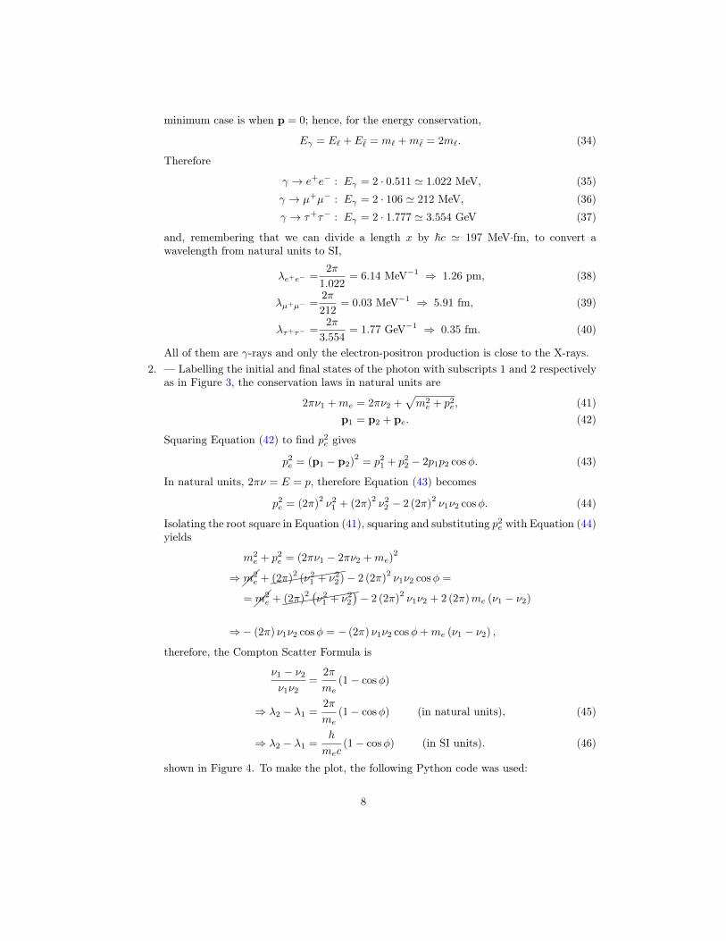
shown in Figure 4. To make the plot, the following Python code was used:

8

0 20 40 60 80 100 120 140 160 180Angle [o ]

0

1

2

3

4

5

λ2−λ

1 [p

m]

Compton Scattering Formula

Figure 4: Plot of the Compton Scatter Formula

import numpy as npimport matplotlib.pyplot as pypfrom scipy.constants import c,h,m_e,pi # h, m_e, c are in SI.

comp = lambda x: 10**12 * h/(m_e*c) * (1-np.cos(x))# 10**12 converts [m] in [pm]x = np.linspace(0,pi,1000) # np.cos has radiant argumentpyp.plot(x*180./pi,comp(x)) # x-axis in degreepyp.xlabel(r"Angle [$^\mathbfo$]",weight="bold")pyp.ylabel(r"$\mathbf\lambda_2 - \lambda_1$ [pm]",weight="bold")pyp.title("Compton Scattering Formula")pyp.savefig("ComptonScatter.eps")pyp.show()

3. — Absorption and photon emission. A γ is absorbed and let the electron of an atomto change in an excited state. When the electron return to its ground state, the atomemits a photon with a characteristic atomic wavelength. This is also called “Fluorescenceradiation”. If the photon energy is enough to unbound the electron from the orbits of theatom, the photoelectric effect occurs.

9

Series 2 – Messengers from the Universe

July 29, 2019

Ex. 1 — Particles from the universeThe flux of the cosmic rays is characterized by a power law due their acceleration mechanismsin their sources: dφ/dE ∝ E−γ . The spectrum index γ is not a constant value for the fullenergy spectrum. Strong debates are around its precise values and the meaning of its evolution,especially for the energy range between E1 = 1018 eV and E2 = 1020 eV.

1. — Calculate the value of the A coefficient, so that the cumulative function of dN/dE isnormalized to 1 between E1 and E2.

2. — Once A is known, write a short python script that generates cosmic rays with a randomenergy E, with E1 ≤ E ≤ E2, according to the flux power law: dN/dE = AE−γ .Plot the obtained energy distribution, using spectrum indices 2 and 3. (Suggestion:Use numpy.random to do the random sampling https://docs.scipy.org/doc/numpy/reference/routines.random.html. In the reference, you will find different methods toperform random extraction, find the one which is more suited for this case.)

3. — Studying the real distribution of the flux of the energy spectrum is still an ongoingresearch. In the scientific article “Measurement of the energy of cosmic rays above 1018 eVusing the Pierre Auger Observatory” you can find a function that describes the spectrumbetween E1 and E2:

J(E;E < Eankle) = BE−γ1 (1)

J(E;E > Eankle) =E−γ2

1 + exp(

log10 E−log10 E1/2

log10Wc

). (2)

Find the values of the needed parameters in the paper. Then generate the random energyof cosmic rays with a distribution in agreement with this function, between E1 and E2.(Suggestion: Use the previous piece of code and re-weight the events with a weight waccording to the function above. Be careful, you need to impose the continuity at Eankle

to find B). Finally, the flux is often multiplied by E2.5 or E3 to observe better its features;use one of these factors to plot your results. Choose the best y-axis to plot the simulatedenergy distribution.

Answer (Ex. 1) —

1

1018 1019 1020

log10(E/eV)

10-1

100

101

102

103

104

105

dN/dE

γ=2

γ=3

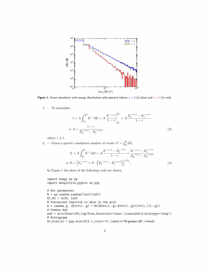
Figure 1: Event simulation with energy distribution with spectral indices γ = 2 (in blue) and γ = 3 (in red).

1. — To normalize,

1 = A

∫ E2

E1

E−γdE = AE−γ+1

1− γ

∣∣∣∣∣

E2

E1

= AE−γ+1

2 − E−γ+11

1− γ

⇒ A =1− γ

E−γ+12 − E−γ+1

1

, (3)

where γ 6= 1.

2. — Given a generic cumulative number of events N =∫ EE1

dE,

N = A

∫ E

E1

E−γdE = AE−γ+1 − E−γ+1

1

1− γ =E−γ+1 − E−γ+1

1

E−γ+12 − E−γ+1

1

⇒ E =[E−γ+1

1 +N ·(E−γ+1

2 − E−γ+11

)] 11−γ

. (4)

In Figure 1 the plots of the following code are shown.

import numpy as npimport matplotlib.pyplot as pyp

# Set parametersR = np.random.random((int)(1e5))E1,E2 = 1e18, 1e20# Convenient function to show in the plotE = lambda g: (E1**(1.-g) + R*(E2**(1.-g)-E1**(1.-g)))**(1./(1.-g))# Common kwdkwd = dict(bins=100,log=True,facecolor=’none’,linewidth=2,histtype=’step’)# HistogramsN1,bins,h1 = pyp.hist(E(2.),color=’b’,label=r"$\gamma=2$",**kwd)

2

N1,bins,h2 = pyp.hist(E(3.),color=’r’,label=r"$\gamma=3$",**kwd)pyp.xscale(’log’)pyp.xlabel(r"$\mathbf\log_10(E/\mathrmeV)$")pyp.ylabel(r"$\mathbf\mathrmdN/\mathrmdE$")pyp.legend()pyp.savefig("simSpectrumIndices.eps")pyp.show()

3. — The smooth function provided by the article from the Pierre Auger collaboration is

J(E;E < Eankle) ∝ E−γ1 (5)

J(E;E > Eankle) ∝ E−γ2

1 + exp(

log10 E−log10 E1/2

log10Wc

), (6)

where the parameters are the following:Parameter Valueγ1 = γ(E < Eankle) 3.26γ2 = γ(E > Eankle) 2.55log10(Eankle/eV) 18.6log10(E1/2/eV) 19.61log10(Wc/eV) 0.16

The idea is to use a simulation from the previous question and re-weight the events witha weight w according to this function. For the continuity,

A · E−γ1ankle =

E−γ2ankle

1 + exp(

log10 Eankle−log10 E1/2

log10Wc

) (7)

⇒ A =Eγ1−γ2ankle

1 + exp(

log10 Eankle−log10 E1/2

log10Wc

), (8)

therefore

w =

Eγ1−γ2ankle

1 + exp(

log10 Eankle−log10 E1/2

log10Wc

) · E−γ1 (E < Eankle)

E−γ2

1 + exp(

log10 E−log10 E1/2

log10Wc

) (E > Eankle)

. (9)

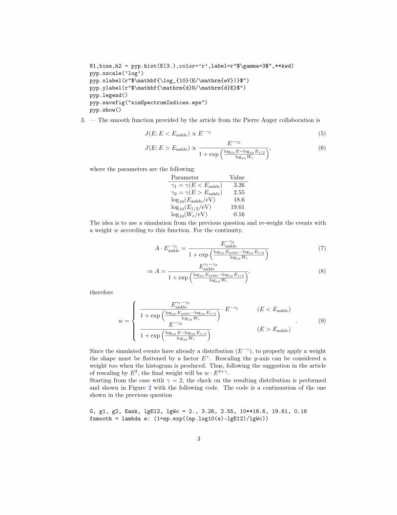
Since the simulated events have already a distribution (E−γ), to properly apply a weightthe shape must be flattened by a factor Eγ . Rescaling the y-axis can be considered aweight too when the histogram is produced. Thus, following the suggestion in the articleof rescaling by E3, the final weight will be w · E3+γ .Starting from the case with γ = 2, the check on the resulting distribution is performedand shown in Figure 2 with the following code. The code is a continuation of the oneshown in the previous question

G, g1, g2, Eank, lgE12, lgWc = 2., 3.26, 2.55, 10**18.6, 19.61, 0.16fsmooth = lambda e: (1+np.exp((np.log10(e)-lgE12)/lgWc))

3

1018 1019 1020

log10(E/eV)

1049

1050

E3·dN/dE

Figure 2: Energy distribution .

A = Eank**(g1-g2)/fsmooth(Eank)Eg2 = E(2.)# Weights for a generic scaleweights = lambda scale: np.where(Eg2>Eank, Eg2**(scale+G-g2)/fsmooth(Eg2),

A*Eg2**(scale+G-g1))# Scale chosen is 3., as said beforeN3,bins,h3 = pyp.hist(Eg2,weights=weights(3.),**kwd)pyp.xscale(’log’)pyp.ylim(ymin=4e48)pyp.xlabel(r"$\mathbf\log_10(E/\mathrmeV)$")pyp.ylabel(r"$\mathbfE^3\!\cdot\,\mathrmdN/\mathrmdE$")pyp.savefig("simSpectrumRealistic.eps")pyp.show()

Ex. 2 — Light from a starWhat is the color of the sun? Looking at it, the answer seems “slightly yellow”, but this is duethe atmospheric filtering of the light1. Since it emits the entire visible region of the electromag-netic spectrum, its color should be “white”. However, it does not emit all the electromagneticfrequencies with the same luminosity.The spectral radiance of a star can be described as a “black-boby radiation”. Therefore, thespectral brightness Iν of the sun, and of a star in general, follows the Plancks’s law for a spectralradiance of a black body. Moreover, its bolometric luminosity is, from the Stefan-Boltzmannlaw, L = 4πσR2

T4eff , where Teff is the effective temperature that characterize the sun2.

1. — Find Teff of the sun. Then, plot writing a short python code its black-body distributionas a function of the wavelength and extract through the code the wavelength and frequency

1The literature terminology “yellow dwarf star” used to classify stars as the sun is a misnomer.2The temperature of a star is not well defined: it is a gradient from the nucleus to the surface and even

in the surface fluctuates quite a lot. Teff define a conventional temperature based on the black body radiancedistribution. Whenever the temperature of a star is cited, it is a reference to this characteristic temperature,which is ∝ 4

√L.

4

of its maximum spectral emission.The spectrum of an astrophysical object is very important because its change (“redshift”)gives hints about the movement of the object.

2. — At the frequency of the emission peak of the sun, give the spectral radiance as calculatedfrom the Planck’s law; calculate then the flux and the luminosity detected on Earth,considering r as the average distance earth-sun. (Suggestion: consider the sun a disc-source perpendicular to the detector, i. e. the earth. . . )

3. — A star equivalent to the sun is moving with β in a direction with angle θ from theobserver.a) Estimate the possible βs with which the object is moving with an apparent speed ≥ c.

(Suggestion: it will be useful to remind the trigonometric identities sinα cosβ +cosα sinβ = sin(α+ β) and cos 45 = sin 45. . . )

b) With the minimum possible β, calculate the ranges of θs and the apparent brightnessfor the peak frequency of the sun.

c) Still with the minimum β but with θ = 180o (i. e. it is going far away from the earth),how much is the redshift?

d) With the previous redshift and assuming a constant Hubble expansion rate H0, howfar is the star from the earth? And with a double redshift?

Answer (Ex. 2) —

1. — From the Stefan-Boltzmann law L = 4πσR2T

4eff , Teff = 5772 K. Knowing the effective

temperature of the sun and the Planck’s law

B (λ, T ) =2hc2

λ5· 1

ehc

λkBTeff − 1(10)

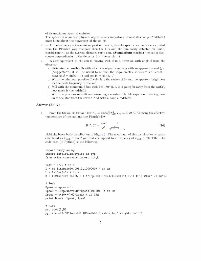
yield the black body distribution in Figure 3. The maximum of this distribution is easilycalculated as λpeek ' 0.502 µm that correspond to a frequency of νpeek ' 597 THz. Thecode used (in Python) is the following:

import numpy as npimport matplotlib.pyplot as pypfrom scipy.constants import h,c,k

Teff = 5772 # in Kl = np.linspace(0.005,3,1000000) # in umL = l*10**(-6) # in mB = ((2*h*c**2)/L**5 ) * 1/(np.e**((h*c)/(L*k*Teff))-1) # in W*sr^-1*m^-3

# PeakBpeak = np.max(B)lpeak = l[np.where(B==Bpeak)[0][0]] # in umfpeak = c*10**(-6)/lpeak # in THzprint Bpeak, lpeak, fpeak

# Plotpyp.plot(l,B)pyp.xlabel(r"$\lambda$ [$\mathbf\lambda$m]",weight=’bold’)

5

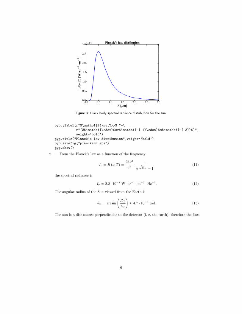
0.0 0.5 1.0 1.5 2.0 2.5 3.0λ [µm]

0.0

0.5

1.0

1.5

2.0

2.5

3.0

B(ν,T

) [W

·sr−1

·m−3

]

1e13 Planck's law ditribution

Figure 3: Black body spectral radiance distribution for the sun.

pyp.ylabel(r"$\mathbfB(\nu,T)$ "+\r"[W$\mathbf\cdot$sr$\mathbf^-1\cdot$m$\mathbf^-3$]",weight=’bold’)

pyp.title("Planck’s law ditribution",weight=’bold’)pyp.savefig("plancksBB.eps")pyp.show()

2. — From the Planck’s law as a function of the frequency

Iν = B (ν, T ) =2hν3

c2· 1

ehν

kBTeff − 1, (11)

the spectral radiance is

Iν ' 2.2 · 10−8 W · sr−1 ·m−2 ·Hz−1. (12)

The angular radius of the Sun viewed from the Earth is

θ = arcsin

(Rr

)≈ 4.7 · 10−3 rad. (13)

The sun is a disc-source perpendicular to the detector (i. e. the earth), therefore the flux

6

is calculated from the integral

Sν =

∫

sun

Iν cos θdθdΩ =

= Iν

∫ 2π

φ=0

∫ θ

θ=0

cos θ sin θdθdφ =

= 2πIν

∫ θ

θ=0

sin θ cos θdθ =

= 2πIν

∫ sin θ

0

xdx =

= πIν sin2 θ, (14)

where dΩ = sin θdθdφ and the substitutions x = sin θ and dx = cos θdθ are used. Sinceθ 1,

Sν ≈ πIνθ2 ≈ 1.52 · 10−12 W ·m−2 ·Hz−1 =

= 152 TJy. (15)

Finally, the luminosity is

Lν = 4πr2Sν ≈ 4.2 · 1011 W ·Hz−1 (16)

3. —a) The apparent βapp is yielded by the formula

βapp =β sin θ

1− β cos θ, (17)

where θ is the angle between the observer and the movement of the star. From theinequality βapp ≥ 1:

1− β cos θ ≤ β sin θ

⇒ 1 ≤ β(sin θ + cos θ)

⇒ 1

β√

2≤ (sin θ cos 45 + cos θ sin 45)

⇒ 0 ≤ 1

β√

2≤ sin(θ + 45) ≤ 1 (18)

⇒ 1√2≤ β ≤ 1. (19)

b) From Equation (19), the minimum possible β is βmin = 1/√

2. From Equation (18),θmin = 45o. For this angle, the only possible, the doppler factor is

δ =

√1− β2

1− β cos θ=√

2. (20)

7

Therefore, since Iν/ν3 is an invariant,

Iemν

ν3em

=Iobsν

ν3obs

=Iobsν

(δνem)3

⇒ Iobsν = δ3Iem

ν ' 6, 2 · 10−8 W · sr−1 ·m−2 ·Hz−1. (21)

c) With θ = 180o, the redshift is simply

z =

√1 + β

1− β − 1 = 1.41. (22)

d) “Same redshift”, means same β. Therefore

βc = H0d (23)

⇒ d =βc

H0' 3127 Mpc. (24)

If the redshift is double, the β will be

z =

√1 + β

1− β − 1

⇒ β =(z + 1)

2 − 1

(z + 1)2

+ 1' 0.87, (25)

therefore

d =βc

H0' 3847 Mpc. (26)

8

Series 3 – Interaction Lengths, Apparent Velocityand Luminosity

July 29, 2019

Ex. 1 — Interaction Length

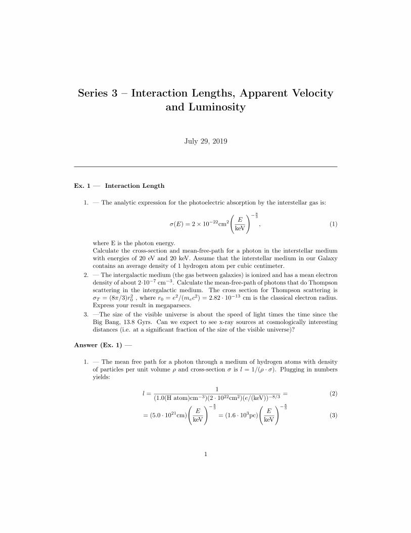
1. — The analytic expression for the photoelectric absorption by the interstellar gas is:

σ(E) = 2× 10−22cm2

(E

keV

)− 83

, (1)

where E is the photon energy.Calculate the cross-section and mean-free-path for a photon in the interstellar mediumwith energies of 20 eV and 20 keV. Assume that the interstellar medium in our Galaxycontains an average density of 1 hydrogen atom per cubic centimeter.

2. — The intergalactic medium (the gas between galaxies) is ionized and has a mean electrondensity of about 2·10−7 cm−3. Calculate the mean-free-path of photons that do Thompsonscattering in the intergalactic medium. The cross section for Thompson scattering isσT = (8π/3)r20 , where r0 = e2/(mec

2) = 2.82 · 10−13 cm is the classical electron radius.Express your result in megaparsecs.

3. —The size of the visible universe is about the speed of light times the time since theBig Bang, 13.8 Gyrs. Can we expect to see x-ray sources at cosmologically interestingdistances (i.e. at a significant fraction of the size of the visible universe)?

Answer (Ex. 1) —

1. — The mean free path for a photon through a medium of hydrogen atoms with densityof particles per unit volume ρ and cross-section σ is l = 1/(ρ · σ). Plugging in numbersyields:

l =1

(1.0(H atom)cm−3)(2 · 1022cm2)(e/(keV))−8/3= (2)

= (5.0 · 1021cm)

(E

keV

)− 83

= (1.6 · 103pc)(

E

keV

)− 83

(3)

1

The cross-sections and mean-free-paths are:

E = 20 eV : σ = 6.8 · 10−18cm2, l = 0.047 pc (4)

E = 20 keV : σ = 6.8 · 10−26cm2, l = 4.7 · 106 pc (5)

2. — The Thompson scattering cross-section is σT = 6.66 · 10−25 cm2 and using the averageelectron density, the mean-free-path is:

l = 1/(ρ · σ) = 7.5 · 1030cm = 2.4 · 106Mpc. (6)

3. — The radius of the visible universe, i.e., the distance a photon can travel since the BigBang, is about the speed of light multiplied by the time since the Big Bang. Since theage of the Universe is 13.8 Gyrs, the radius is 4231 Mpc (including the expansion of theuniverse would increase this by a factor of about 3). Thus, the intergalactic medium istransparent to X-rays.

Ex. 2 — Superluminar motion

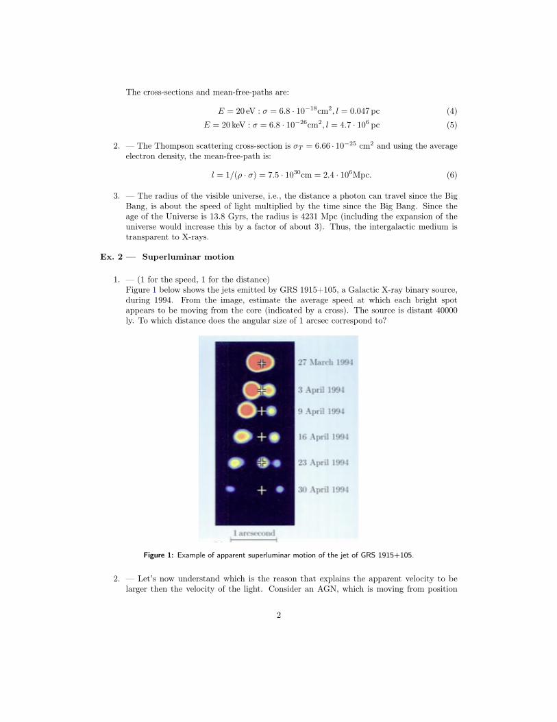
1. — (1 for the speed, 1 for the distance)Figure 1 below shows the jets emitted by GRS 1915+105, a Galactic X-ray binary source,during 1994. From the image, estimate the average speed at which each bright spotappears to be moving from the core (indicated by a cross). The source is distant 40000ly. To which distance does the angular size of 1 arcsec correspond to?

Figure 1: Example of apparent superluminar motion of the jet of GRS 1915+105.

2. — Let’s now understand which is the reason that explains the apparent velocity to belarger then the velocity of the light. Consider an AGN, which is moving from position

2

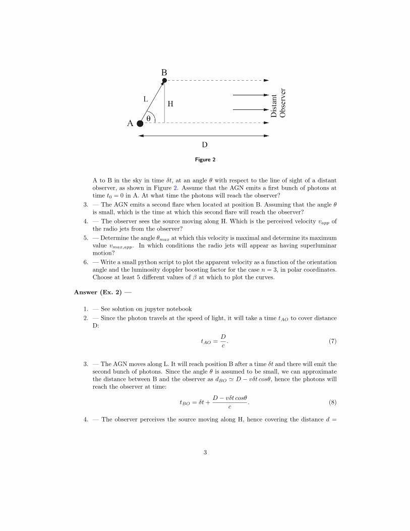
Figure 2

A to B in the sky in time δt, at an angle θ with respect to the line of sight of a distantobserver, as shown in Figure 2. Assume that the AGN emits a first bunch of photons attime t0 = 0 in A. At what time the photons will reach the observer?

3. — The AGN emits a second flare when located at position B. Assuming that the angle θis small, which is the time at which this second flare will reach the observer?

4. — The observer sees the source moving along H. Which is the perceived velocity vapp ofthe radio jets from the observer?

5. — Determine the angle θmax at which this velocity is maximal and determine its maximumvalue vmax,app. In which conditions the radio jets will appear as having superluminarmotion?

6. —Write a small python script to plot the apparent velocity as a function of the orientationangle and the luminosity doppler boosting factor for the case n = 3, in polar coordinates.Choose at least 5 different values of β at which to plot the curves.

Answer (Ex. 2) —

1. — See solution on jupyter notebook2. — Since the photon travels at the speed of light, it will take a time tAO to cover distance

D:

tAO =D

c. (7)

3. — The AGN moves along L. It will reach position B after a time δt and there will emit thesecond bunch of photons. Since the angle θ is assumed to be small, we can approximatethe distance between B and the observer as dBO ' D − vδt cosθ, hence the photons willreach the observer at time:

tBO = δt+D − vδt cosθ

c. (8)

4. — The observer perceives the source moving along H, hence covering the distance d =

3

vδt sinθ, perpendicular to its sight of line with an apparent velocity:

vapp =vδt sinθ

tBO − tAO=

v sinθ

1− vc cosθ

. (9)

5. — The angle that maximizes the apparent jet velocity can be calculated by setting thederivative of vapp(θ) with respect to the angle θ to zero.

v cosθ − v2

ccos2θ − v2

csin2θ = 0, (10)

so that θmax is:

θmax = arccos(vc

). (11)

For v close to the speed of light, this angle is very small. Introducing γ we can obtain anexpression for the maximal observed jet velocity by inserting Eq. 11 into Eq. 9:

vmax,app = γv. (12)

If the jets have velocities close to c, this becomes:

vmax,app = γc, (13)

and this explains how the observed jets velocity can be larger than c even though the truejet speed does not exceed c.

6. — See solution on jupyter notebook

4

Series 4 – Shock waves and Fermi accelerationmechanism

July 29, 2019

Ex. 1 — Fermi acceleration mechanismFermi acceleration mechanisms. In the Fermi acceleration mechanism, charged particles increaseconsiderably their energies crossing back and forth many times the border of a magnetic cloud(second-order Fermi mechanism) or of a shock wave (first-order Fermi mechanism). Computethe number of crossings that a particle must do in each of the mechanisms to have a ratioEfin/Ein = 10, assuming:

1. — realistic values of β = 10−4 for the magnetic cloud and β = 10−2 for the shock wave;2. — β = 10−4 for both acceleration mechanisms.3. — For a CR a realistic mean free path is L ∼ 0.1 pc. Be Φ the pitch angle of the particle

at the i−th scattering. Which is the mean time between collisions? Which would be thetime needed to reach Ef for the magnetic cloud from point 1?

Answer (Ex. 1) —

1. —

∆E1 =Ef,1

E0(1)

∆E2 =Ef,2

Ef,1=

Ef,2

E0 ·∆E1→ Ef,2

E0= ∆E1 ·∆E2 = (∆E)2 (2)

∆En =Ef,2

E0 ·∆E1... ·∆En→ Ef,n

E0= (∆E)n (3)

For the magnetic cloud (β = 10−4) the number of cycles is 1.7 ·108 and for the shock wave(β = 10−2) is 1.7 · 102.

2. — If using β = 10−4 for the shock wave, the number of cycles becomes 1.7 · 104.3. — Define L as mean free path and Φ as pitch angle, the time between collisions is

tcoll =∼ L/(c cosΦ), which can be averaged to 2L/c. Considering L ∼ 0.1 pc and numberof cycles calculated above for the magnetic cloud (β = 10−4), the necessary time shouldbe around 109 years.

1

Ex. 2 — SNR explosions and shock wavesIn SNR explosion shock waves can accelerate particles. A supernova of mass M = 10L (ML =2 · 1033 g) has an ejected mass with typical kinetic energy K ∼ 1051 erg.

1. — How long does it take to extinguish the accelerator (time of free expansion of theejecta)?

Answer (Ex. 2) —

1. — The speed of the shock front can be obtained as:

v =

√2K

M∼ 3200 km/s. (4)

The shock gets extinguished when the mass of the ejecta reach a density equal to theaverage interstellar density ρIG ∼ 1 p/cm3 = 1.6 · 10−24 g/cm3:

ρSN = M/Volume = M/(4/3πR3) = ρIG → Volume→ R ∼ 1.4 · 1019 cm ∼ 5pc. (5)

So the time can be calculated as:

Tacc = R/v ∼ 1000 years (6)

Note that these are only typical order of magnitude numbers.

Ex. 3 — Boron-To-Carbon measurements

1. — Write an approximated Boron production rate due to the Carbon spallation process inthe Galaxy, given its production cross-section σC→B . Given that the Boron productionrate is related to the Boron density by the lifetime of Boron in the Galaxy τ , express theratio NB/NC .

2. — Fit the AMS measurements for the Boron-to-Carbon ratio available in the carbon-boron-AMS02.dat file. (Suggestion: use the log scales on the axes to perform the fit.)

3. — Which is the average interstellar gas number density? Express it in terms of the Boronaverage lifetime in the Galaxy.

Answer (Ex. 3) —

1. — Since we know the partial cross-section of spallation processes we can use the secondary-to-primary abundance ratios to infer the gas column density traversed by the averagecosmic ray. Let us perform a simply estimate of the Boron-to-Carbon ratio. Boron ischiefly produced by Carbon and Oxygen with approximately conserved kinetic energy pernucleon, so we can relate the Boron source production rate, to the differential density ofCarbon by this equation:

QB ∼ nH ·NC · β · c · σC→B (7)

where, nH denotes the average interstellar gas number density, NC is the Carbon density,β is the Carbon velocity and σC→B is the spallation cross-section of Carbon into Boron.

2

The Boron density is related to the production rate by the lifetime of Boron in the Galaxy,τ , before it escapes or losses its energy by spallation QB = NB/τ . So we can write:

NB

NC∼ nH · β · c · σC→B · τ (8)

2. — See Jupiter notebook3. — The values from the are a = 0.44, and b = -0.34. Above about 10 GeV/nucleon the

experimental data can be fitted to a test function, therefore the Boron-to-Carbon ratiocan be expressed as:

NB

NC= 0.4

( EGeV

)−0.3(9)

For energies above 10 GeV/nucleon we can approximate β ∼ 1, which leads, using thevalues of the cross-section, to a life time gas density of:

nH · τ ∼ 1014( EGeV

)−0.3s cm−3 (10)

3