arX

iv:0

707.

4210

v1 [

mat

h.G

T]

28

Jul 2

007

Sampling Lissajous and Fourier Knots

Adam Boocher∗

University of Notre Dame

Jay Daigle∗

Pomona College

Jim Hoste∗

Pitzer College

Wenjing Zheng∗

University of California, Berkeley

October 31, 2018

Abstract

A Lissajous knot is one that can be parameterized as

K(t) = (cos(nxt+ φx), cos(nyt+ φy), cos(nzt+ φz))

where the frequencies nx, ny , and nz are relatively prime integers and the phase shifts φx, φy and φz arereal numbers. Lissajous knots are highly symmetric, and for this reason, not all knots are Lissajous. Weprove several theorems which allow us to place bounds on the number of Lissajous knot types with givenfrequencies and to efficiently sample all possible Lissajous knots with a given set of frequencies. In par-ticular, we systematically tabulate all Lissajous knots with small frequencies and as a result substantiallyenlarge the tables of known Lissajous knots.

A Fourier-(i, j, k) knot is similar to a Lissajous knot except that the x, y and z coordinates are noweach described by a sum of i, j and k cosine functions respectively. According to Lamm, every knot is aFourier-(1, 1, k) knot for some k. By randomly searching the set of Fourier-(1, 1, 2) knots we find that all2-bridge knots up to 14 crossings are either Lissajous or Fourier-(1, 1, 2) knots. We show that all twistknots are Fourier-(1, 1, 2) knots and give evidence suggesting that all torus knots are Fourier-(1, 1, 2)knots.

As a result of our computer search, several knots with relatively small crossing numbers are identifiedas potential counterexamples to interesting conjectures.

∗Supported by NSF REU grant DMS-0453284.

1

1 Introduction

A Lissajous knot K in R3 is a knot that has a parameterization K(t) = (x(t), y(t), z(t)) given by

x(t) = cos(nxt+ φx)y(t) = cos(nyt+ φy)z(t) = cos(nzt+ φz)

where 0 ≤ t ≤ 2π, nx, ny, and nz are integers, and φx, φy , φz ∈ R.

Lissajous knots were first studied in [1] where some of their elementary properties were established. Mostnotably, Lissajous knots enjoy a high degree of symmetry. In particular, if the three frequencies nx, ny andnz (which must be pairwise relatively prime—see [1]) are all odd, then the knot is strongly plus amphicheiral.If one of the frequencies is even, then the knot is 2-periodic, with the additional property that it links itsaxis of rotation once. These symmetry properties imply (strictly) weaker properties such as the fact thatthe Alexander polynomial of a Lissajous knot must be a square mod 2, which in turn implies that its Arfinvariant must be zero. See [1], [7] and [11] for details. Thus for example, the trefoil and figure eight knotsare not Lissajous since their Arf invariants are one. In fact, “most” knots are not Lissajous.

To date it is unknown if every knot which is strongly plus amphicheiral or 2-periodic (and links its axis ofrotation once) is Lissajous. Several knots with relatively few crossings exist which meet these symmetryrequirements and yet are still unknown to be Lissajous or not. For example, according to [6] there are onlythree prime knots with 12 or less crossings which are strongly plus amphicheiral: 10a103 (1099), 10a121(10123), and 12a427. Here we have given knot names in both the Dowker-Thistlethwaite ordering of theHoste-Thistlethwaite-Weeks table [6] and, in parenthesis, the Rolfsen [14] ordering (for knots with 10 or lesscrossings). Symmetries of the knots in the Hoste-Thistlethwaite-Weeks table were computed using SnapPeaas described in [6]. Of these three knots, only 10a103 (1099) was previously reported as Lissajous. (See [10]and [11].) However we find 12a427 to be Lissajous. (See Section 5 of this paper.) This leaves open the caseof 10a121. As a further example, there are exactly four 8-crossings knots which are 2-bridge, 2-periodic,and link their axis of rotation once. Despite our extensive searching (see Section 5) only one of these knotsturned up as Lissajous (and it had already been reported as such in [10]). Whether the other three areLissajous remains unknown.

Lissajous knots are a subset of the more general class of Fourier knots. A Fourier-(i, j, k) knot is one thatcan be parameterized as

x(t) = Ax,1 cos(nx,1t+ φx,1) + ...+Ax,i cos(nx,it+ φx,i)y(t) = Ay,1 cos(ny,1t+ φy,1) + ...+Ay,j cos(ny,jt+ φy,j)z(t) = Az,1 cos(nz,1t+ φz,1) + ...+Az,k cos(nz,kt+ φz,k).

Because any function can be closely approximated by a sum of cosines, every knot is a Fourier knot for some(i, j, k). But a remarkable theorem of Lamm [10] states that in fact every knot is a Fourier-(1, 1, k) knotfor some k. While k cannot equal one for all knots (these are the Lissajous knots, and not all knots areLissajous) could k possibly be less than some universal bound M for all knots? This seems unlikely, withthe more reasonable outcome being that k depends on the specific knot K. Yet no one has found a knot forwhich k must be bigger than two!

If K is a Fourier-(1, 1, k) knot then its bridge number is less than or equal to the minimum of nx and ny.(The bridge number of a knot K can be defined as the smallest number of extrema on K with respect toa given direction in R

3, taken over all representations of K and with respect to all directions. See [2] or[14] for more details.) Moreover, Lamm’s proof is constructive and explicitly shows that if K has bridgenumber b, then K is a Fourier-(1, 1, k) knot for some k and with nx = b. This raises several interestingquestions. For any knot K, when expressed as a Fourier-(1, 1, k) knot, can the minimum values of nx and k

2

be simultaneously realized? In particular, can a knot which is Lissajous and with bridge index b be realizedas a Lissajous knot with nx = b?

Let L(nx, ny, nz) be the set of all Lissajous knots with frequencies nx, ny, nz. (Throughout this paper weconsider a knot and its mirror image to be equivalent.) One of the main goals of this paper is to investigatethe set L(nx, ny, nz). By a simple change of variables, t → t+ c, we may alter the phase shifts. Therefore wewill assume that φx = 0 in all that follows. This leaves the pair of parameters (φy, φz) which vary within thephase torus [0, 2π]× [0, 2π]. In Section 2 we examine the phase torus and identify a finite number of regionsin which the phase shifts must lie, with each region corresponding to a single knot type. We further showthat a periodic pattern of knot types are produced as one traverses the phase torus. This allows us to prove

Theorem 1. Let |L(nx, ny, nz)| be the number of distinct Lissajous knots with frequencies (nx, ny, nz). Then

|L(nx, ny, nz)| ≤ 2nxny.

If furthermore nx = 2, then|L(2, ny, nz)| ≤ 2ny + 1.

There is also a periodicity that exists across frequencies and in Section 2 we also prove

Theorem 2. L(nx, ny, nz) ⊆ L(nx, ny, nz + 2nxny), with equality if nz ≥ 2nxny − ny.

Our analysis of the phase torus, together with these theorems allow us to efficiently sample (with the aid ofa computer) all possible Lissajous knots having two of the three frequencies bounded. Even with relativelysmall frequencies, the three natural projections of a Lissajous knot into the three coordinate planes canhave a large number of crossings. (The projection into the xy-plane has 2nxny − nx − ny crossings.) Withfrequencies of 10 or more, diagrams with hundreds of crossings result and many, if not most, knot invariantsare computationally out of reach. Thus it becomes extremely difficult to compare different Lissajous knotswith large frequencies, or to try to locate them in existing knot tables. However, if one frequency is two,the knot is 2-bridge and even with hundreds of crossings it is relatively simple to compute the identifyingfraction p/q by which 2-bridge knots are classified.

In Section 2 we recall basic facts about Lissajous knots and prove several theorems, including the two alreadymentioned, that will allow us to efficiently sample all Lissajous knots with two given frequencies. In Section 4we then recall some basic facts about 2-bridge knots. Using these results we then report in Section 5 on ourcomputer experiments. Theorems similar to those given in Section 2 but for Fourier-(1, 1, k) knots wouldnecessarily be much more complicated and we only begin the analysis of the phase torus for Fourier-(1, 1, 2)knots in Section 3. Without the analogous results, we have not been able to rigorously sample Fourier knots.Instead, we have proceeded by two methods, either random sampling, or a sampling based on first forminga bitmap image of the phase torus and its singular curves. However, even without exhaustive sampling, ourdata show that all 2-bridge knots up to 14 crossings are Fourier-(1, 1, k) knots with k ≤ 2 and with nx = 2.

This research was carried out at the Claremont College’s REU program in the summer of 2006. The authorsthank the National Science Foundation and the Claremont Colleges for their generous support.

2 The Phase Torus—Lissajous Knots

Suppose K(t) is a Lissajous knot and consider its diagram in the xy-plane. Each crossing in this diagramcorresponds to a double point in the xy-projection given by a pair of times (t1, t2), where x(t1) = x(t2) andy(t1) = y(t2). The following lemma is given in [7].

3

-1 -0.5 0.5 1

-1

-0.5

0.5

1

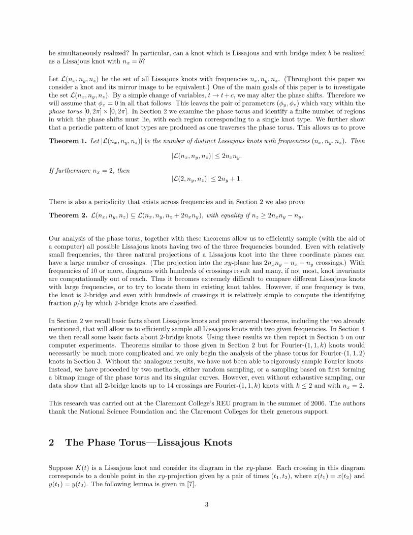
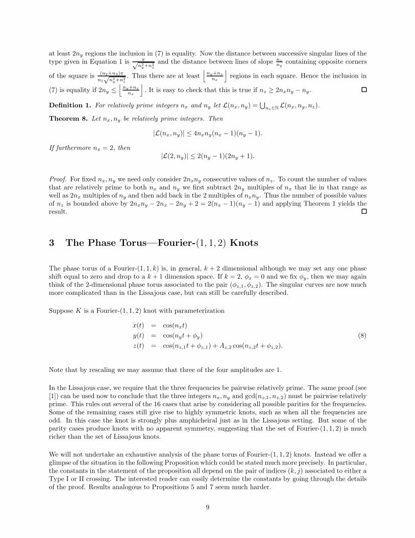
Figure 1: A Lissajous knot with frequencies (3, 5, 7) and corresponding phase shifts (0, π/4, π/12). The TypeI crossings appear in two rows with five crossings each and the Type II crossings appear in four columnswith three crossings each.

Lemma 3. Let K(t) be a Lissajous knot. There are two types of time pairs (t1, t2) that give double pointsin the xy-projection:

Type I : (t1, t2) =(

(− knx

+ jny

)π − φy

ny

, ( knx

+ jny

)π − φy

ny

)

1 ≤ k ≤ nx − 1, 1 + ⌊ny

nx

k +φy

π ⌋ ≤ j ≤ ⌊2ny − ny

nx

k +φy

π ⌋

Type II : (t1, t2) =(

(− kny

+ jnx

)π − φx

nx

, ( kny

+ jnx

)π − φx

nx

)

1 ≤ k ≤ ny − 1, 1 + ⌊nx

ny

k + φx

π ⌋ ≤ j ≤ ⌊2nx − nx

ny

k + φx

π ⌋

There are nxny − ny double points of Type I, and nxny − nx double points of Type II.

Figure 1 shows a Lissajous knot with frequencies (3, 5, 7) and corresponding phase shifts (0, π/4, π/12). Sinceall the frequencies are odd, this knot is symmetric through the origin. It is not hard to show that in general,the Type I crossings line up in sets of size ny on nx − 1 horizontal lines, while the Type II crossings line upin sets of size nx on ny − 1 vertical lines. If nx = 2 there is a single row of Type I crossings, all of which lieon the x-axis and ny − 1 columns of Type II crossings with each column consisting of two crossings.

Not all phase shift pairs will generate curves that are knots. Assuming φx = 0, the knot K(t) will intersectitself, and thus fail to be a knot, exactly when the phase shifts satisfy

φz =nz

nyφy + l

π

ny, or (1)

φz = lπ

nx, or (2)

φy = lπ

nx(3)

for some integer l. Crossings of Type I become singular precisely when Equation 1 holds; crossings of TypeII when Equaton 2 holds. When Equation 3 holds, the entire xy-projection degenerates to an arc. Whilethis alone does not imply the knot has points of self-intersection, this is indeed the case. See [8, 1, 7] formore details. In Proposition 5, we specifically identify which crossings become singular as the phase shiftsmove across these lines.

The slanted, horizontal and vertical lines given in Equations 1–3 obviously divide the phase torus into regionswith each region defining one knot type. Thus there are only a finite number of knots types possible fora given set of frequencies. There is, however, a great deal of repetition in knot types as one traverses thephase torus due to the periodicity of the cosine function. The following theorem describes a nice choice of“fundamental domain” on the phase torus to which we may restrict our attention.

4

Theorem 4. Any knot in L(nx, ny, nz) can be represented with φx = 0 and using some phase shift pair(φy , φz) in [0, π

nx

]× [0, π].

Proof. Define an equivalence relation ∼ on the phase torus for L(nx, ny, nz) by (φy, φz) ∼ (φ′y , φ

′z) if the

Lissajous knot with phase shifts (0, φy, φz) is the same as the knot with phase shifts (0, φ′y, φ

′z), or its mirror

image. Clearly(φy , φz) ∼ (φy ± π, φz) ∼ (φy , φz ± π). (4)

If K ∈ L(nx, ny, nz), a change of variable t → t+ πnx

shows that K is also parameterized as

x = − cos(nxt)y = cos(nyt+ φy +

nyπnx

)

z = cos(nzt+ φz +nzπnx

).

Therefore we also have(φy , φz) ∼ (φy +

nyπ

nx, φz +

nzπ

nx). (5)

Now since nx and ny are relatively prime, there are integers k and l with 0 ≤ φy +knyπnx

− lπ < πnx

. Repeat-edly using (4) and (5) we obtain

(φy, φz) ∼ (φy +knyπ

nx− lπ, φz +

knzπ

nx)

The first coordinate is already in [0, πnx

]; we can shift the second coordinate by multiples of π until it is in[0, π]. Thus an arbitrary point (φy, φz) is equivalent to some point in [0, π

nx

]× [0, π], as desired.

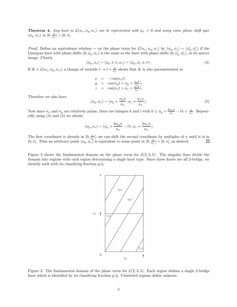
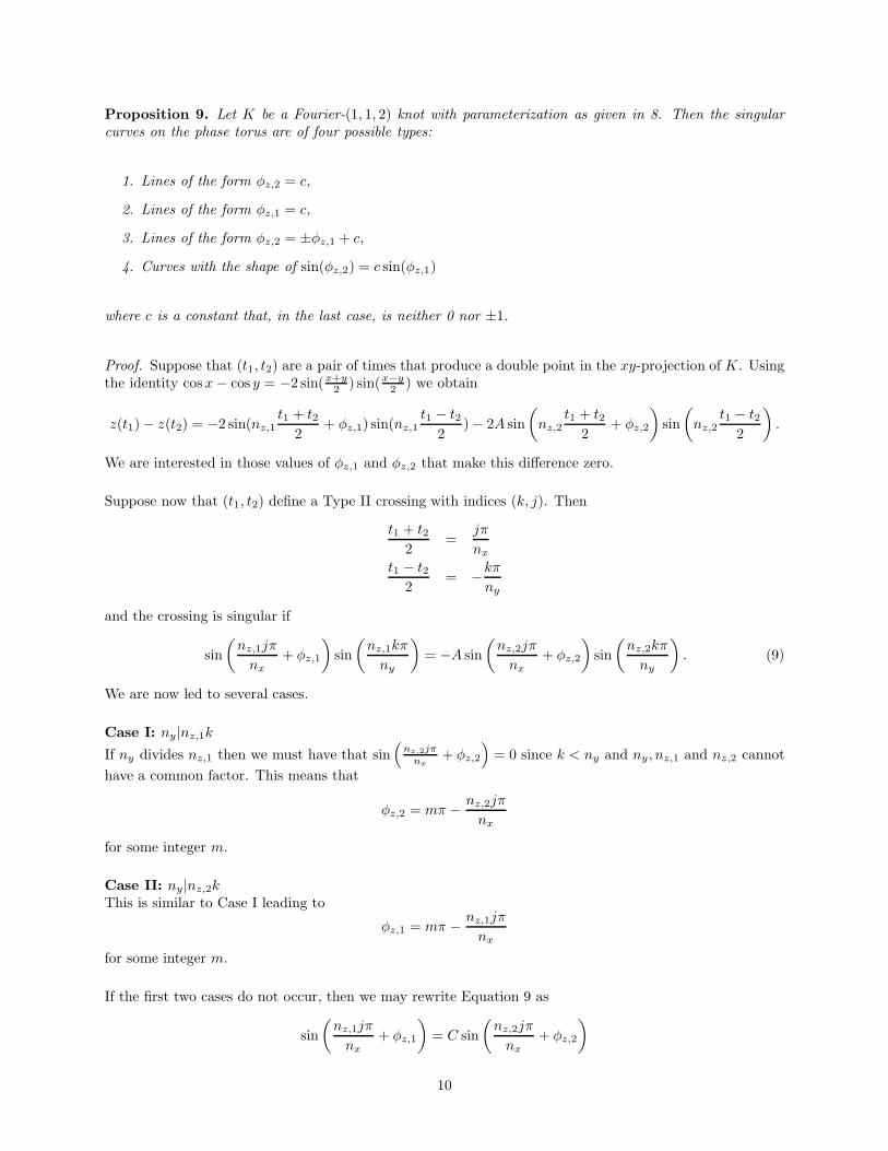
Figure 2 shows the fundamental domain on the phase torus for L(2, 3, 5). The singular lines divide thedomain into regions with each region determining a single knot type. Since these knots are all 2-bridge, weidentify each with its classifying fraction p/q.

PSfrag replacements

9/2

9/2

7/2

7/2

π

π2

0 π2

φz

φy

Figure 2: The fundamental domain of the phase torus for L(2, 3, 5). Each region defines a single 2-bridgeknot which is identified by its classifying fraction p/q. Unlabeled regions define unknots.

5

Our next result specifically describes what happens as we cross a singular line of the type given in Equation 1or 2.

Proposition 5. Let K and K ′ be two Lissajous knots with frequencies (nx, ny, nz) and phase shifts (φy , φz)and (φ′

y , φ′z) respectively.

1. Suppose (φy , φz) and (φ′y , φ

′z) lie in two adjacent regions of the phase torus separated by a diagonal line

L given by φz = nz

ny

φy + l πny

. Then K and K ′ differ by changing all Type I crossings with parameters

(k, j) such that with jnz + l ≡ 0 mod ny. The number of such crossings is nx − 1.

2. Suppose (φy , φz) and (φ′y, φ

′z) lie in two adjacent regions of the phase torus separated by a horizontal

line L given by φz = l πnx

. Then K and K ′ differ by changing all Type II crossings with parameters(k, j) such that jnz + l ≡ 0 mod nx. The number of such crossings is ny − 1.

Proof. If (t1, t2) is a Type I crossing with parameters (k, j), then z(t1) = z(t2) if and only if

cos(nzt1 + φz) = cos(nzt2 + φz)

which will occur if and only if

nz(t1 − t2) = 2mπ or nz(t1 + t2) + 2φz = 2m′π (6)

for some integers m,m′. For Type I crossings,

t1 − t2 = − 2k

nxπ and t1 + t2 =

2j

nyπ − 2φy

ny.

If (6) is to hold, then in the first case, we have

−2knz

nxπ = 2mπ

which is equivalent to −knz = mnx. This is impossible since nx and nz are relatively prime and 1 ≤ k ≤nx − 1.

In the second case, we have

nz

(

2j

nyπ − 2

φy

ny

)

+ 2φz = 2m′π

which is equivalent to

φz =nz

nyφy + (m′ny − jnz)

π

ny.

Thus Type I crossings only become singular on lines of the form given in Equation 1 with l = mny − jnz.

If φz = nz

nx

φy + l πny

+ ε and jnz + l = mny for some integer m then it is straightforward to check that

z(t1)− z(t2) = (−1)m2 sin ε sinknzπ

nx.

Hence, as we move across the line L by letting ε go from a small positive value to a small negative value, thedifference z(t1)− z(t2) changes sign. Thus the Type I crossings with parameters (k, j) actually change fromover to under or vice versa, rather than simply becoming singular and then “rebounding” to their originalpositions.

Finally, note that once l is fixed this does not necessarily uniquely determine j and thus the correspondingType I crossing. If both jnz+ l ≡ 0 mod ny and j′nz+ l ≡ 0 mod ny then j ≡ j′ mod ny since ny and nz are

6

relatively prime. If nx = 2, then k = 1 and j lies in an interval of length ny. Thus with nx = 2 we have thatj is uniquely determined by l and a single crossing changes as we move across L. But if nx > 2 and k = 1then j lies in an interval of length greater than ny. Hence two admissible values, j and j + ny, are possible.

Using j, we must have 1 ≤ k ≤⌊

nx

ny

(j − φy

π )⌋

while for j + ny we must have 1 ≤ k ≤⌊

nx

ny

(−j + ny +φy

π )⌋

.

Thus the total number of possible points (k, j) is⌊

nx

ny

(j − φy

π )⌋

+⌊

nx

ny

(−j + ny +φy

π )⌋

= nx − 1.

A similar discussion handles the Type II crossings.

Corollary 6. Suppose K and K ′ are Lissajous knots with frequencies (nx, ny, nz) and phase shifts whichbelong to regions separated by 2ny singular lines of the type given in Equation 1. Then all Type I crossingsare the same for both knots.

Proof. From Proposition 5 we know that crossing the line φz = nz

ny

φy + l πny

changes exactly those Type I

crossings with parameters (k, j) for which jnz+l ≡ 0 mod ny. Thus if we cross the singular line correspondingto l and then later cross the line corresponding to l+ny the same set of Type I crossings will first be changedand then changed back again. Hence, after crossing over 2ny such lines all Type I crossings will be restoredto their original position.

If nx = 2 there is even more repetition due to additional symmetry as is shown in the following result.

Proposition 7. Let K and K ′ be Lissajous knots with frequencies (2, ny, nz) and phase shifts (φy , φz) and(φ′

y , φ′z) respectively. If (φy , φz) and (φ′

y, φ′z) are symmetric with respect to the point (π/4, π/4) or the point

(π/4, 3π/4) then K and K ′ are equivalent.

Proof. Suppose (φy , φz) and (φ′y , φ

′z) are symmetric with respect to the point (π/4, π/4). Then φ′

y = π/2−φy

and φ′z = π/2− φz. Thus

K ′(−t+ π/2) = (cos(−2t+ π), cos(−nyt+ nyπ/2 + π/2− φy), cos(−nzt+ nzπ/2 + π/2− φz)

= (− cos(2t), (−1)(ny+1)/2 cos(nyt+ φy), (−1)(nz+1)/2 cos(nzt+ φz))

which is either K(t) or its mirror image K(t).

The second case follows similarly.

We may now prove Theorem 1.

Proof of Theorem 1: The fundamental domain is divided into nx “boxes” of the form[0, π

nx

]× [k πnx

, (k+1) πnx

] for 0 ≤ k ≤ nx − 1. Within each box all the knots have the same Type II crossingsand hence by Corollary 6 there are at most 2ny different knot types in that box. Since there are nx boxeswe obtain at most 2nxny different knots.

If nx = 2 there is the additional rotational symmetry in each box given by Proposition 7. The center of eachbox either lies on a slanted singular line, or midway between two such lines. Moreover, one of the two boxeswill be one way and the other box will be the other way. There are at most ny knot types in the box wherethe center of the box lies on a singular line, and there are at most ny + 1 knot types in the box otherwise.Thus there are at most 2ny + 1 knot types in total.

7

Our results thus far allow us to efficiently sample all Lissajous knots with a given set of frequencies(nx, ny, nz). We can easily pick one set of phase shifts from each region on the phase torus and Corol-lary 6, and Proposition 7 in the case when nx = 2, allows us to further restrict the regions that we mustsample. However, once nx, ny, and φy are given, the xy-projection has been fixed and it is natural to ask ifall possible choices for nz are necessary. Theorem 2, which is stated in the introduction, shows that in fact,only a finite number of values for nz are needed to produce all possible knots.

Proof of Theorem 2: Suppose that K ∈ L(nx, ny, nz), K′ ∈ L(nx, ny, nz + 2nxny) and that both knots

have the same phase shifts. We will show first that each knot has its Type II crossings arranged the sameway.

Let (t1, t2) be a Type II crossing with parameters (k, j) and let

∆II(nx, ny, nz, φz , k, j) = cos(nzt1 + φz)− cos(nzt1 + φz)

= 2 sin

(

nz

(

t1 + t22

)

+ φz

)

sin

(

nz

(

t1 − t22

))

= −2 sin

(

nzjπ

nx+ φz

)

sin

(

nzkπ

ny

)

be the height difference between the two points on the knot directly above the crossing.

It is easy to verify that

∆II(nx, ny, nz, φz , k, j) = ∆II(nz + 2nxny, ny, nz, φz , k, j) for all k, j.

Thus if nz is increased by 2nxny, not only do all Type II crossings remain unchanged, they each maintainthe same height difference between upper and lower strand.

We now shift our focus to Type I crossings. Let K have phase shifts (φy,nz

ny

φy − ε) and choose ε small

enough so that K corresponds to the region just below the singular line φz = nz

ny

φy. Let K ′ correspond to

the “same” region, that is, let K ′ have phase shifts (φy ,nz+2nxny

ny

φy − ε). As before, let (t1, t2) be a Type I

crossing with parameters (k, j) and let

∆I(nx, ny, nz, φy, φz , k, j) = cos(nzt1 + φz)− cos(nzt1 + φz)

= 2 sin

(

nz

(

t1 + t22

)

+ φz

)

sin

(

nz

(

t1 − t22

))

= −2 sin

(

nzjπ

ny− nzφy

ny+ φz

)

sin

(

nzkπ

nx

)

be the height difference between the two points on the knot directly above the crossing. It is easy to checkthat

∆(nx, ny, nz,nz

nyφy − ε, k, j) = ∆(nx, ny, nz + 2nxny,

nz + 2nxny

nyφy − ε, k, j).

Thus K and K ′ are the same knot since both the Type I and Type II crossings are arranged the same wayin each. If the phase shifts for K are now changed by moving into an adjacent region, and if the phase shiftsfor K ′ are changed in the same way, then the same set of crossings is changed for both K and K ′ and henceK and K ′ remain the same knot. Therefore

L(nx, ny, nz) ⊆ L(nx, ny, nz + 2nxny). (7)

According to Corollary 6, the pattern of knot types in each square [0, π/nx]×[kπ/nx, (k+1)π/nx], as we movefrom the upper left corner to the lower right corner, is periodic with period 2ny. Thus if each box contains

8

at least 2ny regions the inclusion in (7) is equality. Now the distance between successive singular lines of thetype given in Equation 1 is π√

n2y+n2

z

and the distance between lines of slope nz

ny

containing opposite corners

of the square is (n2+n3)π

n1

√n2y+n2

z

. Thus there are at least⌊

ny+nz

nx

⌋

regions in each square. Hence the inclusion in

(7) is equality if 2ny ≤⌊

ny+nz

nx

⌋

. It is easy to check that this is true if nz ≥ 2nxny − ny.

Definition 1. For relatively prime integers nx and ny let L(nx, ny) =⋃

nz∈NL(nx, ny, nz).

Theorem 8. Let nx, ny be relatively prime integers. Then

|L(nx, ny)| ≤ 4nxny(nx − 1)(ny − 1).

If furthermore nx = 2, then|L(2, ny)| ≤ 2(ny − 1)(2ny + 1).

Proof. For fixed nx, ny we need only consider 2nxny consecutive values of nz. To count the number of valuesthat are relatively prime to both nx and ny we first subtract 2ny multiples of nx that lie in that range aswell as 2nx multiples of ny and then add back in the 2 multiples of nxny. Thus the number of possible valuesof nz is bounded above by 2nxny − 2nx − 2ny + 2 = 2(nx − 1)(ny − 1) and applying Theorem 1 yields theresult.

3 The Phase Torus—Fourier-(1, 1, 2) Knots

The phase torus of a Fourier-(1, 1, k) is, in general, k + 2 dimensional although we may set any one phaseshift equal to zero and drop to a k + 1 dimension space. If k = 2, φx = 0 and we fix φy , then we may againthink of the 2-dimensional phase torus associated to the pair (φz,1, φz,2). The singular curves are now muchmore complicated than in the Lissajous case, but can still be carefully described.

Suppose K is a Fourier-(1, 1, 2) knot with parameterization

x(t) = cos(nxt)

y(t) = cos(nyt+ φy) (8)

z(t) = cos(nz,1t+ φz,1) +Az,2 cos(nz,2t+ φz,2).

Note that by rescaling we may assume that three of the four amplitudes are 1.

In the Lissajous case, we require that the three frequencies be pairwise relatively prime. The same proof (see[1]) can be used now to conclude that the three integers nx, ny and gcd(nz,1, nz,2) must be pairwise relativelyprime. This rules out several of the 16 cases that arise by considering all possible parities for the frequencies.Some of the remaining cases still give rise to highly symmetric knots, such as when all the frequencies areodd. In this case the knot is strongly plus amphicheiral just as in the Lissajous setting. But some of theparity cases produce knots with no apparent symmetry, suggesting that the set of Fourier-(1, 1, 2) is muchricher than the set of Lissajous knots.

We will not undertake an exhaustive analysis of the phase torus of Fourier-(1, 1, 2) knots. Instead we offer aglimpse of the situation in the following Proposition which could be stated much more precisely. In particular,the constants in the statement of the proposition all depend on the pair of indices (k, j) associated to either aType I or II crossing. The interested reader can easily determine the constants by going through the detailsof the proof. Results analogous to Propositions 5 and 7 seem much harder.

9

Proposition 9. Let K be a Fourier-(1, 1, 2) knot with parameterization as given in 8. Then the singularcurves on the phase torus are of four possible types:

1. Lines of the form φz,2 = c,

2. Lines of the form φz,1 = c,

3. Lines of the form φz,2 = ±φz,1 + c,

4. Curves with the shape of sin(φz,2) = c sin(φz,1)

where c is a constant that, in the last case, is neither 0 nor ±1.

Proof. Suppose that (t1, t2) are a pair of times that produce a double point in the xy-projection of K. Usingthe identity cosx− cos y = −2 sin(x+y

2 ) sin(x−y2 ) we obtain

z(t1)− z(t2) = −2 sin(nz,1t1 + t2

2+ φz,1) sin(nz,1

t1 − t22

)− 2A sin

(

nz,2t1 + t2

2+ φz,2

)

sin

(

nz,2t1 − t2

2

)

.

We are interested in those values of φz,1 and φz,2 that make this difference zero.

Suppose now that (t1, t2) define a Type II crossing with indices (k, j). Then

t1 + t22

=jπ

nx

t1 − t22

= −kπ

ny

and the crossing is singular if

sin

(

nz,1jπ

nx+ φz,1

)

sin

(

nz,1kπ

ny

)

= −A sin

(

nz,2jπ

nx+ φz,2

)

sin

(

nz,2kπ

ny

)

. (9)

We are now led to several cases.

Case I: ny|nz,1k

If ny divides nz,1 then we must have that sin(

nz,2jπnx

+ φz,2

)

= 0 since k < ny and ny, nz,1 and nz,2 cannot

have a common factor. This means that

φz,2 = mπ − nz,2jπ

nx

for some integer m.

Case II: ny|nz,2kThis is similar to Case I leading to

φz,1 = mπ − nz,1jπ

nx

for some integer m.

If the first two cases do not occur, then we may rewrite Equation 9 as

sin

(

nz,1jπ

nx+ φz,1

)

= C sin

(

nz,2jπ

nx+ φz,2

)

10

0 50 100 150 200 250

0

50

100

150

200

250

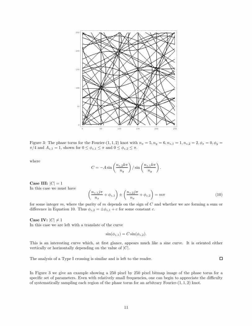
Figure 3: The phase torus for the Fourier-(1, 1, 2) knot with nx = 5, ny = 6, nz,1 = 1, nz,2 = 2, φx = 0, φy =π/4 and Az,1 = 1, shown for 0 ≤ φz,1 ≤ π and 0 ≤ φz,2 ≤ π.

where

C = −A sin

(

nz,2kπ

ny

)

/ sin

(

nz,1kπ

ny

)

.

Case III: |C| = 1In this case we must have

(

nz,1jπ

nx+ φz,1

)

±(

nz,2jπ

nx+ φz,2

)

= mπ (10)

for some integer m, where the parity of m depends on the sign of C and whether we are forming a sum ordifference in Equation 10. Thus φz,2 = ±φz,1 + c for some constant c.

Case IV: |C| 6= 1In this case we are left with a translate of the curve

sin(φz,1) = C sin(φz,2).

This is an interesting curve which, at first glance, appears much like a sine curve. It is oriented eithervertically or horizontally depending on the value of |C|.

The analysis of a Type I crossing is similar and is left to the reader.

In Figure 3 we give an example showing a 250 pixel by 250 pixel bitmap image of the phase torus for aspecific set of parameters. Even with relatively small frequencies, one can begin to appreciate the difficultyof systematically sampling each region of the phase torus for an arbitrary Fourier-(1, 1, 2) knot.

11

4 2-Bridge Knots

Every 2-bridge knot can be classified by a pair of relatively prime integers (p, q) such that p is odd and0 < q < p. We will often write the pair (p, q) as the fraction p/q. If Kp/q and Kp′/q′ are two 2-bridgeknots with corresponding fractions p/q and p′/q′ then they are equivalent knots if and only if p = p′ and±q′q±1 ≡ 1 mod p. The reader is referred to [2] for details.

If K is a Fourier (1, 1, 2) knot with nx = 2 then K is a 2-bridge knot. We may recover the fraction p/q fromthe Lissajous projection in the xy-plane as follows. This projection is a 4-plat diagram. As we move in thex-direction from left to right we see a single Type I crossings on the x-axis, then a pair of Type II crossingswhich are symmetric with respect to the x-axis, then another Type I crossing on the x-axis, and so on. Letη1, η2, . . . be the signs of the Type I crossings from left to right along the x-axis. Let {ε11, ε21}, {ε12, ε22}, . . .be the signs of the pairs of Type II crossings from left to right. Proceeding in a fashion similar to that givenon pages 300–303 in [14], we obtain that p/q is given by the continued fraction

p/q = [η1, ε11 + ε21, η2, ε

12 + ε22, . . . , ηny

] = η1 +1

ε11 + ε21 +1

η2 + · · ·+1

ηny

(11)

Note that if K is Lissajous then it is rotationally symmetric with respect to the x-axis and each pair of TypeII crossings has the same sign. In this case each ε1i + ε2i can be replaced with 2ε1i . Using this formula, it iseasy to determine the 2-bridge knot given by a Fourier-(1, 1, 2) representation with nx = 2. Hence, when wesample Lissajous and Fourier-(1, 1, 2) knots with nx = 2, even if we obtain knots with hundreds of crossings,it is a simple matter to distinguish them.

Since every Lissajous knot with nx = 2 is 2-bridge, a good question is: What 2-bridge knots are Lissajouswith nx = 2? As mentioned in the Introduction, every Lissajous knot is either strongly plus amphicheiral,or 2-periodic and linking its axis of rotation once. It is known that a 2-bridge knot cannot be strongly plusamphicheiral [4]. It is also known (and will be shown below) that every 2-bridge knot is 2-periodic, but mayor may not link its axis of rotation once. The following theorem makes it easy to identify which 2-bridgeknots might be Lissajous.

Theorem 10. Let K be a 2-bridge knot. Then the following are equivalent.

1) K has a symmetry of period 2 with axis A such that A is disjoint from K and |lk(A,K)| = 1

2) ∆K(t) is a square mod 2

3) ∆K(t) ≡ 1 mod 2.

Proof. As already mentioned in the introduction, it follows from a result of Murasugi (see [12]) that 1)implies 2) and clearly 3) implies 2). We must show that 2) implies both 1) and 3).

Suppose K is a 2-bridge knot given by the pair of relatively prime integers (p, q) with p odd and 0 < q < p.There is a unique continued fraction expansion

p/q = [2a1,−2a2, . . . , (−1)n+12an]

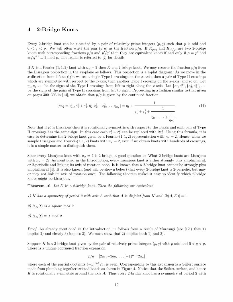
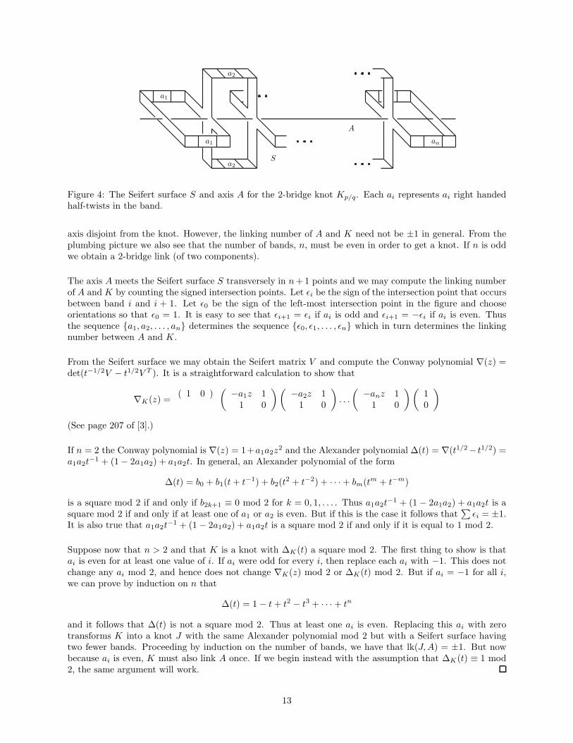
where each of the partial quotients (−1)i+12ai is even. Corresponding to this expansion is a Seifert surfacemade from plumbing together twisted bands as shown in Figure 4. Notice that the Seifert surface, and henceK is rotationally symmetric around the axis A. Thus every 2-bridge knot has a symmetry of period 2 with

12

PSfrag replacements

a1

a1

a2

a2S

A

an

Figure 4: The Seifert surface S and axis A for the 2-bridge knot Kp/q. Each ai represents ai right handedhalf-twists in the band.

axis disjoint from the knot. However, the linking number of A and K need not be ±1 in general. From theplumbing picture we also see that the number of bands, n, must be even in order to get a knot. If n is oddwe obtain a 2-bridge link (of two components).

The axis A meets the Seifert surface S transversely in n+1 points and we may compute the linking numberof A and K by counting the signed intersection points. Let ǫi be the sign of the intersection point that occursbetween band i and i + 1. Let ǫ0 be the sign of the left-most intersection point in the figure and chooseorientations so that ǫ0 = 1. It is easy to see that ǫi+1 = ǫi if ai is odd and ǫi+1 = −ǫi if ai is even. Thusthe sequence {a1, a2, . . . , an} determines the sequence {ǫ0, ǫ1, . . . , ǫn} which in turn determines the linkingnumber between A and K.

From the Seifert surface we may obtain the Seifert matrix V and compute the Conway polynomial ∇(z) =det(t−1/2V − t1/2V T ). It is a straightforward calculation to show that

∇K(z) =( 1 0 )

(

−a1z 11 0

)(

−a2z 11 0

)

. . .

(

−anz 11 0

)(

10

)

(See page 207 of [3].)

If n = 2 the Conway polynomial is ∇(z) = 1+a1a2z2 and the Alexander polynomial ∆(t) = ∇(t1/2− t1/2) =

a1a2t−1 + (1− 2a1a2) + a1a2t. In general, an Alexander polynomial of the form

∆(t) = b0 + b1(t+ t−1) + b2(t2 + t−2) + · · ·+ bm(tm + t−m)

is a square mod 2 if and only if b2k+1 ≡ 0 mod 2 for k = 0, 1, . . . . Thus a1a2t−1 + (1 − 2a1a2) + a1a2t is a

square mod 2 if and only if at least one of a1 or a2 is even. But if this is the case it follows that∑

ǫi = ±1.It is also true that a1a2t

−1 + (1− 2a1a2) + a1a2t is a square mod 2 if and only if it is equal to 1 mod 2.

Suppose now that n > 2 and that K is a knot with ∆K(t) a square mod 2. The first thing to show is thatai is even for at least one value of i. If ai were odd for every i, then replace each ai with −1. This does notchange any ai mod 2, and hence does not change ∇K(z) mod 2 or ∆K(t) mod 2. But if ai = −1 for all i,we can prove by induction on n that

∆(t) = 1− t+ t2 − t3 + · · ·+ tn

and it follows that ∆(t) is not a square mod 2. Thus at least one ai is even. Replacing this ai with zerotransforms K into a knot J with the same Alexander polynomial mod 2 but with a Seifert surface havingtwo fewer bands. Proceeding by induction on the number of bands, we have that lk(J,A) = ±1. But nowbecause ai is even, K must also link A once. If we begin instead with the assumption that ∆K(t) ≡ 1 mod2, the same argument will work.

13

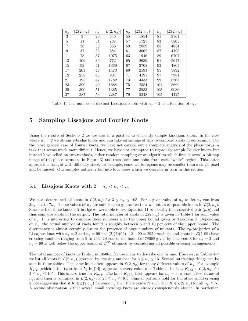
ny |L(2, ny)| ny |L(2, ny)| ny |L(2, ny)| ny |L(2, ny)|3 3 29 645 55 1854 81 37615 11 31 737 57 1727 83 58057 28 33 533 59 2859 85 46549 37 35 684 61 3062 87 419511 78 37 1075 63 1946 89 670713 109 39 772 65 2639 91 564715 93 41 1339 67 3708 93 480517 203 43 1473 69 2593 95 589219 258 45 904 71 4191 97 798421 195 47 1782 73 4433 99 520823 390 49 1688 75 2584 101 869925 390 51 1365 77 3933 103 903627 387 53 2287 79 5248 105 4425

Table 1: The number of distinct Lissajous knots with nx = 2 as a function of ny.

5 Sampling Lissajous and Fourier Knots

Using the results of Sections 2 we are now in a position to efficiently sample Lissajous knots. In the casewhere nx = 2 we obtain 2-bridge knots and can take advantage of this to compare knots in our sample. Forthe more general case of Fourier knots, we have not carried out a complete analysis of the phase torus, atask that seems much more difficult. Hence, we have not attempted to rigorously sample Fourier knots, butinstead have relied on two methods, either random sampling or an algorithm which first “draws” a bitmapimage of the phase torus (as in Figure 3) and then picks one point from each “white” region. This latterapproach is fraught with difficulty since, for example, some white regions may be smaller than a single pixeland be missed. Our samples naturally fall into four cases which we describe in turn in this section.

5.1 Lissajous Knots with 2 = nx < ny < nz

We have determined all knots in L(2, ny) for 3 ≤ ny ≤ 105. For a given value of ny we let nz run from3ny + 2 to 7ny. These values of nz are sufficient to guarantee that we obtain all possible knots in L(2, ny).Since each of these knots is 2-bridge we were able to use Equation 11 to identify the associated pair (p, q) andthus compare knots in the output. The total number of knots in L(2, ny) is given in Table 1 for each valueof ny. It is interesting to compare these numbers with the upper bound given by Theorem 8. Dependingon ny, the actual number of knots found is roughly between 5 and 10 per cent of the upper bound. Thediscrepancy is almost certainly due to the presence of huge numbers of unknots. The xy-projection of aLissajous knot with nx = 2 and ny = 99 has (2)(2)(99)− 2− 99 = 295 crossings, and knots in L(2, 99) havecrossing numbers ranging from 5 to 293. Of course the bound of 78008 given by Theorem 8 for nx = 2 andny = 99 is well below the upper bound of 2295 obtained by considering all possible crossing arrangements!

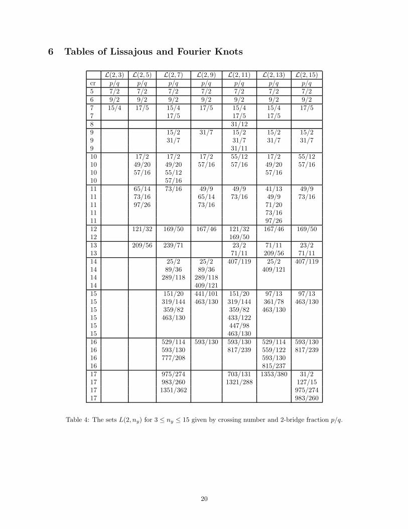
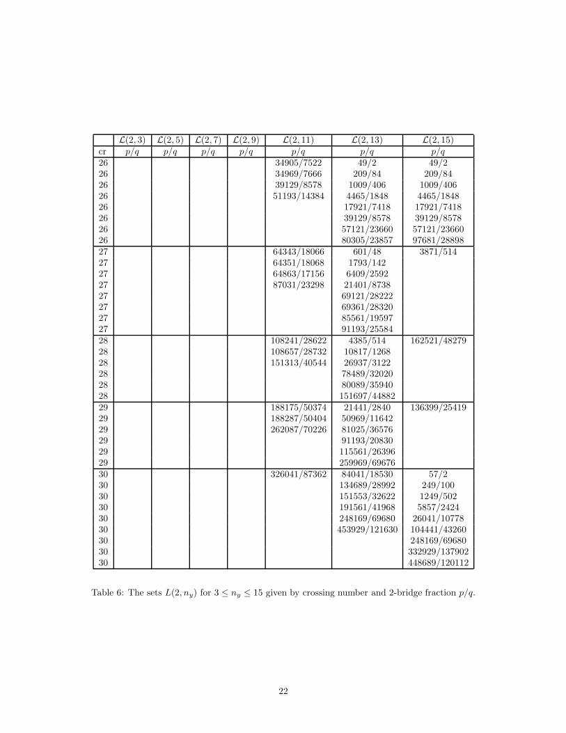
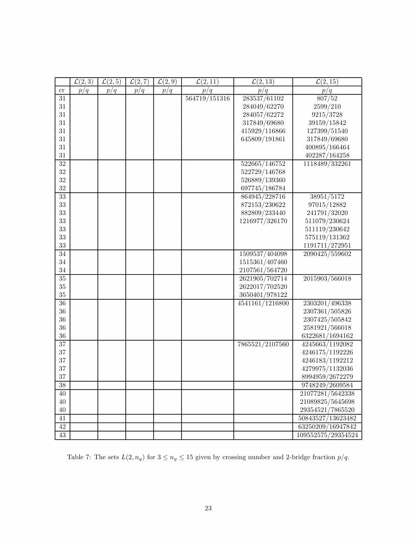
The total number of knots in Table 1 is 135061, far too many to describe one by one. However, in Tables 4–7we list all knots in L(2, ny), grouped by crossing number, for 3 ≤ ny ≤ 15. Several interesting things can beseen in these tables. The same knot often appears in L(2, ny) for many different values of ny. For exampleK7/2 (which is the twist knot 52 in [14]) appears in every column of Table 4. In fact, K7/2 ∈ L(2, ny) for3 ≤ ny ≤ 105. This is also true for K9/2. The knot K15/4 first appears for ny = 3, misses a few values ofny, and then is contained in L(2, ny) for 23 ≤ ny ≤ 105. Similar patterns hold for the other small-crossingknots suggesting that if K ∈ L(2, ny) for some ny then there exists N such that K ∈ L(2, ny) for all ny ≥ N .A second observation is that several small crossings knots are already conspicuously absent. In particular,

14

there are exactly four 8-crossings knots with Alexander polynomial congruent to 1 mod 2 (and hence possiblyLissajous). These are K17/4,K23/7,K25/9 and K31/12, only one of which, K31/12, appears to be Lissajous.While Tables 4–7 display only a small fraction of our total sample, it is in fact true that the other three8-crossing knots do not appear for any ny up to 105.

Question 1. Does there exist a 2-bridge knot K with ∆K(t) ≡ 1 mod 2 that is not Lissajous (with orwithout one frequency equal to 2)? In particular, are any of the 8-crossing 2-bridge knots K17/4,K23/7 orK25/9 Lissajous?

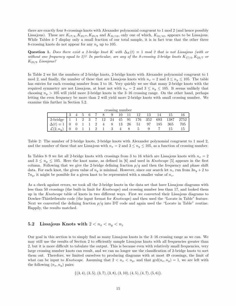
In Table 2 we list the numbers of 2-bridge knots, 2-bridge knots with Alexander polynomial congruent to 1mod 2, and finally, the number of these that are Lissajous knots with nx = 2 and 3 ≤ ny ≤ 105. The tablehas entries for each crossing number from 3 to 16. Very quickly we see that many 2-bridge knots with therequired symmetry are not Lissajous, at least not with nx = 2 and 3 ≤ ny ≤ 105. It seems unlikely thatchoosing ny > 105 will yield more 2-bridge knots in the 3–16 crossing range. On the other hand, perhapsletting the even frequency be more than 2 will yield more 2-bridge knots with small crossing number. Weexamine this further in Section 5.2.

crossing number3 4 5 6 7 8 9 10 11 12 13 14 15 16

2-bridge 1 1 2 3 7 12 24 45 91 176 352 693 1387 2752∆(t) ≡ 1 0 0 1 1 2 4 8 13 26 51 97 185 365 705L(2, ny) 0 0 1 1 2 1 3 4 8 5 9 7 15 15

Table 2: The number of 2-bridge knots, 2-bridge knots with Alexander polynomial congruent to 1 mod 2,and the number of these that are Lissajous with nx = 2 and 3 ≤ ny ≤ 105, as a function of crossing number.

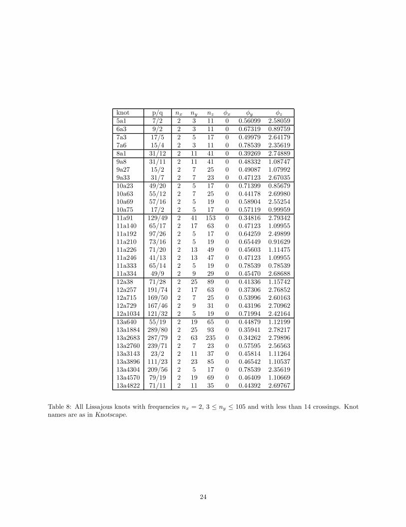
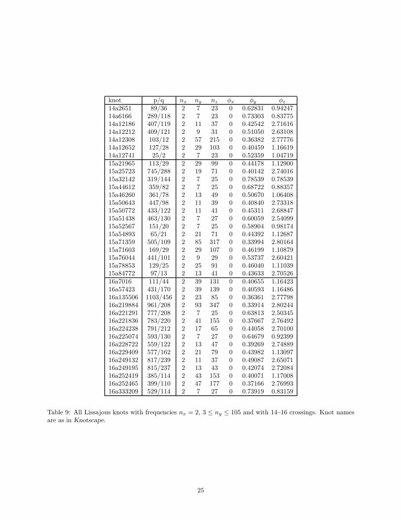
In Tables 8–9 we list all 2-bridge knots with crossings from 3 to 16 which are Lissajous knots with nx = 2and 3 ≤ ny ≤ 105. Here the knot name, as defined in [6] and used in Knotscape [5] appears in the firstcolumn. Following that we give the 2-bridge defining fraction p/q and then the frequency and phase shiftdata. For each knot, the given value of ny is minimal. However, since our search let nz run from 3ny + 2 to7ny, it might be possible for a given knot to be represented with a smaller value of nz.

As a check against errors, we took all the 2-bridge knots in the data set that have Lissajous diagrams withless than 50 crossings (the built-in limit for Knotscape) and crossing number less than 17, and looked themup in the Knotscape table of knots in two different ways. First we converted their Lissajous diagrams toDowker-Thistlethwaite code (the input format for Knotscape) and then used the “Locate in Table” feature.Next we converted the defining fraction p/q into DT code and again used the “Locate in Table” routine.Happily, the results matched.

5.2 Lissajous Knots with 2 < nx < ny < nz

Our goal in this section is to simply find as many Lissajous knots in the 3–16 crossing range as we can. Wemay still use the results of Section 2 to efficiently sample Lissajous knots with all frequencies greater than2, but it is more difficult to tabulate the output. This is because even with relatively small frequencies, verylarge crossing number knots can result, and we can no longer use the classification of 2-bridge knots to sortthem out. Therefore, we limited ourselves to producing diagrams with at most 49 crossings, the limit ofwhat can be input to Knotscape. Assuming that 2 < nx < ny, and that gcd(nx, ny) = 1, we are left withthe following (nx, ny) pairs:

{(3, 4), (3, 5), (3, 7), (3, 8), (3, 10), (4, 5), (4, 7), (5, 6)}.

15

For each of these pairs we let nz run from 2nxny − nx − ny to 4nxny − nx − ny − 1, a range sufficient toproduce all possible Lissajous knots. We obtained a total of 6352 knots of which Knotscape identified 1428as unknots. The remaining 4924 knots fell into four categories:

1. knots identified as composites by Knotscape,

2. knots which Knotscape located in the Hoste-Thistlethwaite-Weeks table,

3. knots which Knotscape simplified to alternating projections with more than 16 crossings, and

4. knots which Knotscape simplified to nonalternating projections with more than 16 crossings.

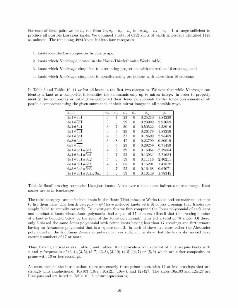
In Table 3 and Tables 10–11 we list all knots in the first two categories. We note that while Knotscape canidentify a knot as a composite, it identifies the summands only up to mirror image. In order to properlyidentify the composites in Table 3 we compared their Jones polynomials to the Jones polynomials of allpossible composites using the given summands or their mirror images in all possible ways.

knot nx ny nz φx φy φz

3a1#3a1 3 4 23 0 0.25210 1.842293a1#3a1 3 5 29 0 0.23099 2.910595a1#5a1 3 7 50 0 0.50522 1.589165a1#5a1 3 5 29 0 0.26179 1.832596a1#6a1 4 5 37 0 0.18699 2.954596a3#6a3 3 8 47 0 0.23799 0.809196a3#6a3 3 5 29 0 0.29259 0.754593a1#3a1#5a1 4 5 39 0 0.16064 2.195543a1#3a1#5a1 4 7 55 0 0.13934 2.216843a1#3a1#8a2 5 6 59 0 0.11116 2.402115a1#5a1#5a1 4 7 55 0 0.15201 1.418786a3#6a3#6a3 4 7 55 0 0.16468 0.620713a1#3a1#3a1#3a1 5 6 59 0 0.10149 1.78345

Table 3: Small-crossing composite Lissajous knots. A bar over a knot name indicates mirror image. Knotnames are as in Knotscape.

The third category cannot include knots in the Hoste-Thistlethwaite-Weeks table and we make no attemptto list them here. The fourth category might have included knots with 16 or less crossings that Knotscape

simply failed to simplify correctly. To investigate this we first computed the Jones polynomial of each knotand eliminated knots whose Jones polynomial had a span of 17 or more. (Recall that the crossing numberof a knot is bounded below by the span of the Jones polynomial.) This left a total of 78 knots. Of these,only 5 shared the same Jones polynomial with prime knots having less than 17 crossings and furthermorehaving an Alexander polynomial that is a square mod 2. In each of these five cases either the Alexanderpolynomial or the Kauffman 2-variable polynomial was sufficient to show that the knots did indeed havecrossing numbers of 17 or more.

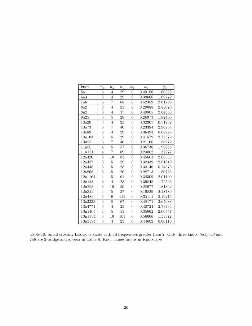
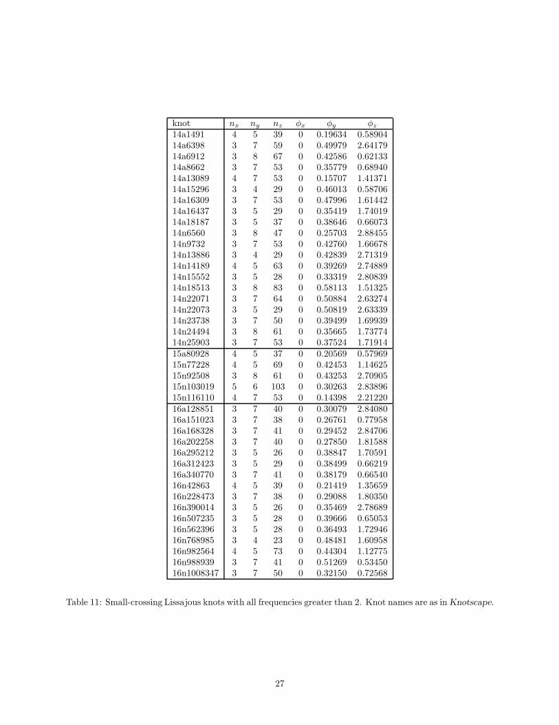
Thus, barring clerical errors, Table 3 and Tables 10–11 provide a complete list of all Lissajous knots withx and y frequencies of (3, 4), (3, 5), (3, 7), (3, 8), (3, 10), (4, 5), (4, 7) or (5, 6) which are either composite, orprime with 16 or less crossings.

As mentioned in the introduction, there are exactly three prime knots with 12 or less crossings that arestrongly plus amphicheiral: 10a103 (1099), 10a121 (10123), and 12a427. The knots 10a103 and 12a427 areLissajous and are listed in Table 10. A natural question is,

16

Question 2. Is the strongly plus amphicheiral knot 10a121 Lissajous?

The knot 10a121 is one member of a family of knots known as Turks Head knots. These knots are conjecturedto not be Lissajous by Przytycki. See [13].

It is easy to see that every composite knot of the form K#K is strongly plus amphicheiral while compositesof the form K#K are 2-periodic and link their axis of rotation once. Several knots of this form appear inTable 3. Thus another good question is,

Question 3. Is every composite knot of the form K#K or K#K Lissajous?

5.3 Fourier-(1, 1, 2) Knots with 2 = nx < ny

Rather than trying to algorithmically choose one point in each region of the phase torus for a Fourier-(1, 1, 2)knot, we chose instead to randomly sample points from the phase torus. Fixing nx = 2, φx = 0 and Az,1 = 1,we then let ny take on odd values from 3 to 99. For each value of ny the remaining parameters were thenchosen at random such that:

φy = k7π, k ∈ {1, 2, 3, 4, 5, 6}

0 < nz,1 < nz,2 < 3010 ≤ φz,1 ≤ π0 ≤ φz,2 ≤ 2π0 ≤ Az,2 ≤ 2

For each value of ny, random sampling in batches of 10000 took place until no new knots were found. If a knotwas produced that had already been found, the one with the lexicographically smallest set {nx, ny, nz,1, nz,2}was kept. This tended to produce knots with fairly small values of {nx, ny, nz,1 but with nz,2 often in thehundreds. Furthermore, only knots with less than 17 crossings were kept in the sample.

After a modest amount of searching, we turned up all 2-bridge knots with 14 or less crossings, and nearlyall 15 and 16-crossing ones as well. (We found 1386 out of 1387 15-crossing knots and 2731 out of 275216-crossing knots.) We believe the following conjecture is reasonable.

Conjecture 11. Every 2-bridge knot can be expressed as a Fourier-(1, 1, k) knot with nx = 2 and k ≤ 2.

Additional evidence for this conjecture is provided by the twist knots. The twist knot Tm, which is the2-bridge knot K 2m+1

2

, is shown in Figure 5. The mirror image of Tm is the twist knot T−1−m. Thus it

suffices to consider m > 1. It is shown in [7] that Tm is Lissajous if and only if m ≡ 0 mod 4 or m ≡ 3mod 4. If this is not the case, the knot does not have the required symmetry to be Lissajous. However,in these cases, the following examples show that Km is a Fourier-(1, 1, 2) knot. Thus all twist knots areFourier-(1, 1, k) knots with k ≤ 2.

Theorem 12. Twist knots which are not Lissajous may be expressed as Fourier knots as follows.

1. The twist knot T4n+1 can be expressed as the Fourier-(1, 1, 2) knot with nx = 2, φx = 0, ny = 8n+3, φy =

1/2, nz,1 = 2, φz,1 = π/4, nz,2 = 8n+ 1, φz,2 = 8n+1+(8n+5)π2(8n+3) and Az,2 = 1 for all n ≥ 1.

2. The twist knot T2n can be expressed as the Fourier-(1, 1, 2) knot with nx = 2, φx = 0, ny = 2n+1, φy =1/2, nz,1 = 2, φz,1 = π/4, nz,2 = 2n+ 3, φz,2 = 2n+3−3π

2(2n+1) and Az,2 = 1 for all n ≥ 1.

17

The proof is similar to the proof of Theorem 4 given in [7] and relies on very carefully determining the signof each crossing in the diagram. The details are quite long and not particularly insightful. We leave this asa rather complicated exercise for the reader.

Figure 5: The twist knot Tm.

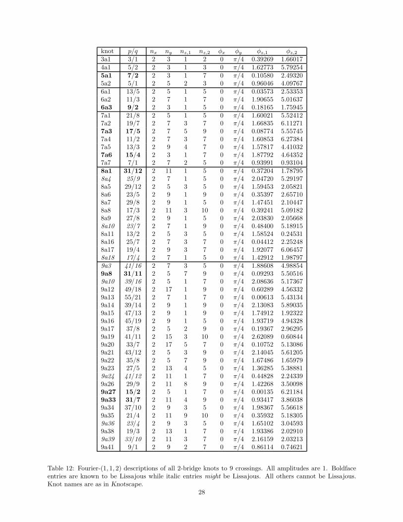
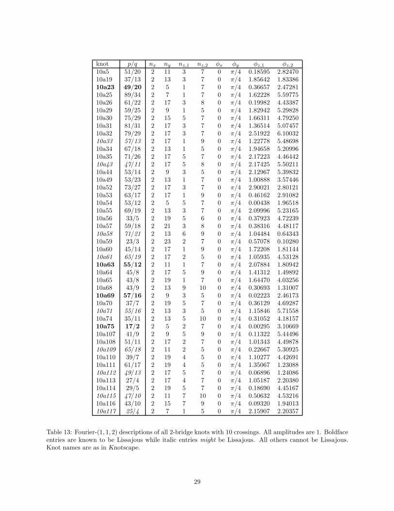
Our sample of all 2-bridge knots to 16 crossings expressed as Fourier-(1, 1, 2) knots is too large to reproducehere. Instead, in Tables 12–13 we list all 2-bridge knots to 10 crossings with associated Fourier data. Togenerate this table we again undertook a random sample but this time sharply reduced the range of theparameters. In particular, we kept all amplitudes equal to one, set φy = π/4, and only allowed z-frequenciesas large as 10. An interesting variation on Conjecture 11 would be to require that all amplitudes are 1.Knots appearing in Tables 12–13 which are known to be Lissajous are shown in boldface, while those thathave Alexander polynomials congruent to 1 mod 2, and hence might be Lissajous, are shown in italics.

5.4 Fourier-(1, 1, 2) Knots with 2 < nx < ny

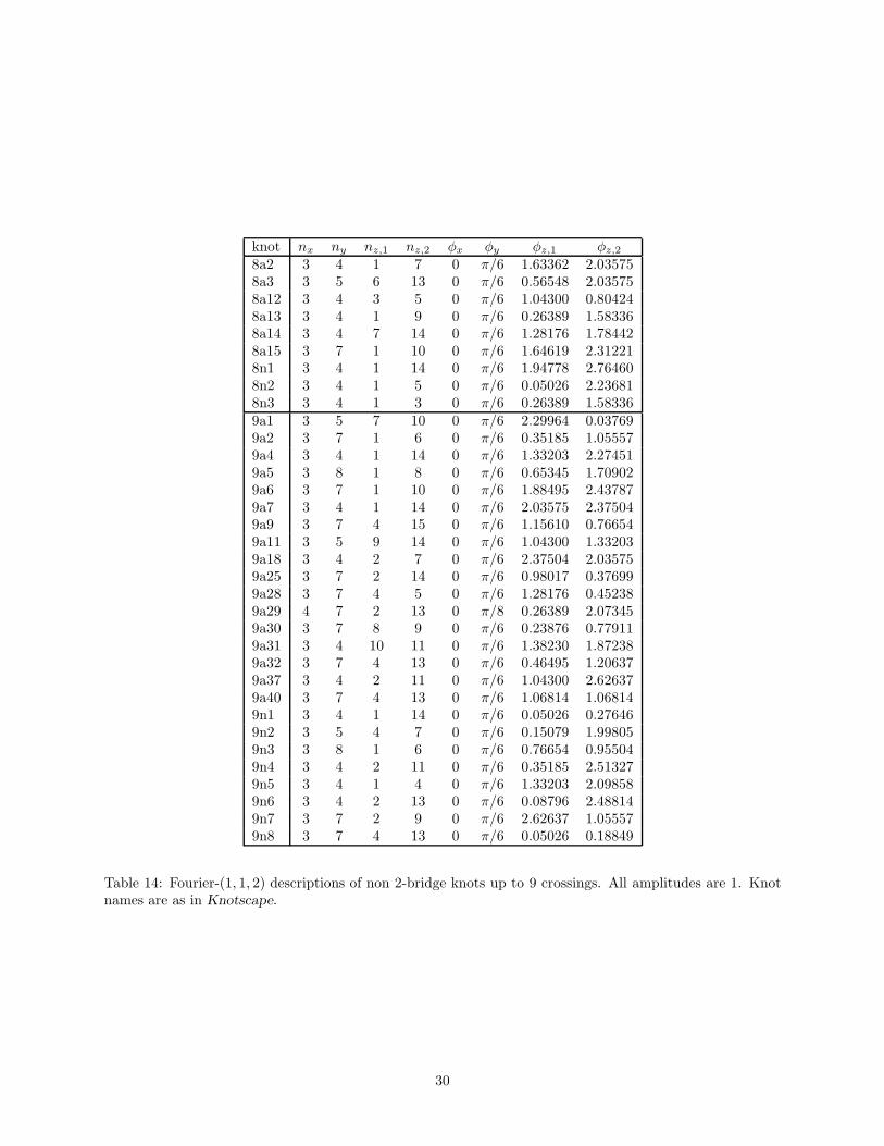
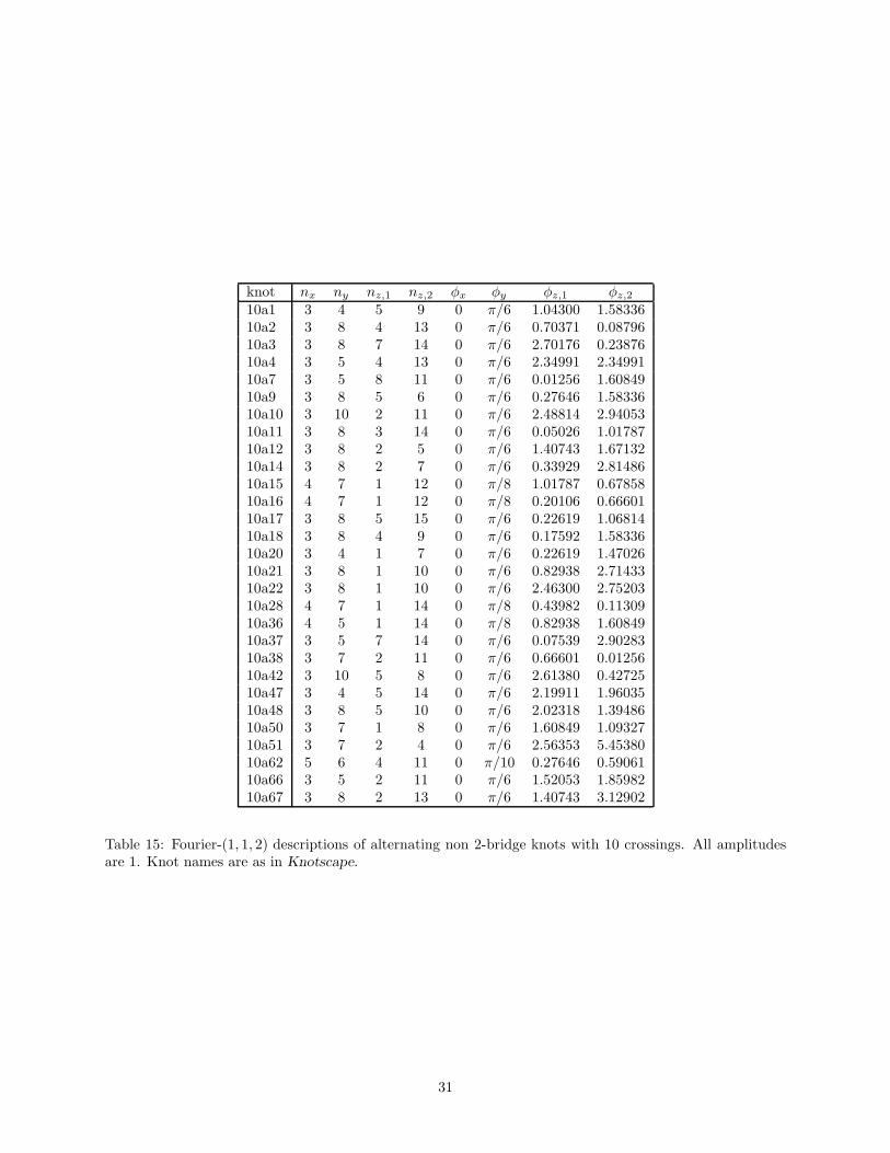
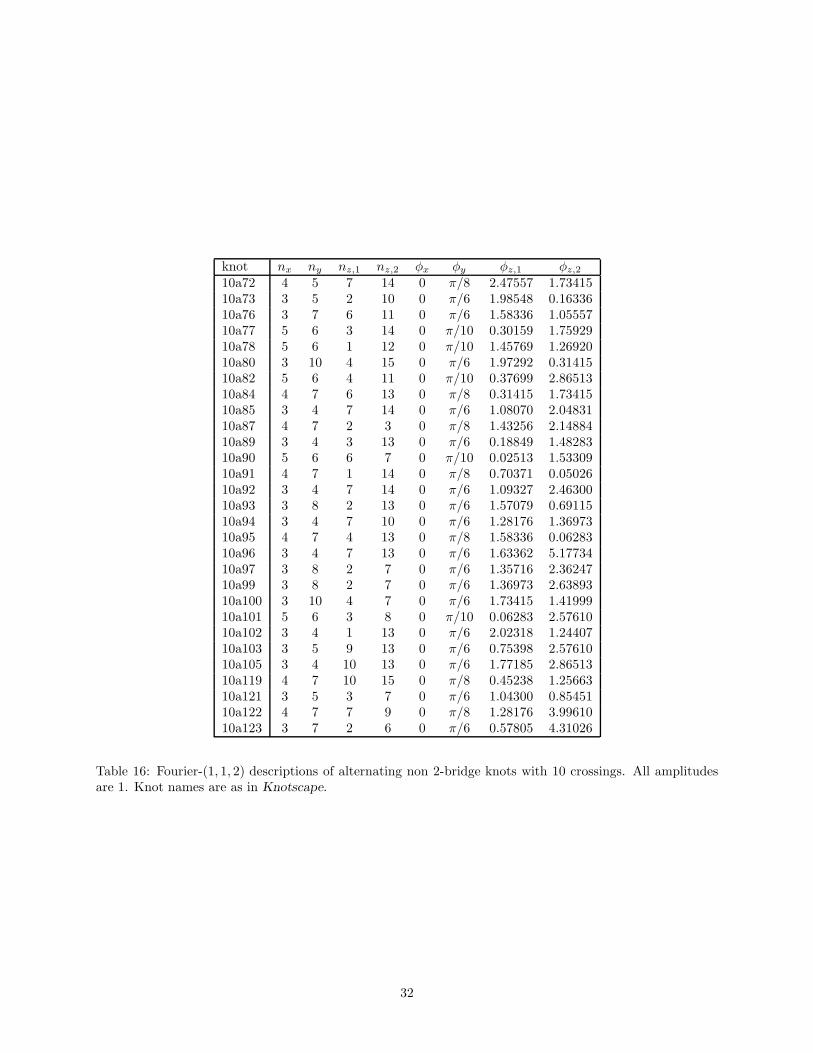
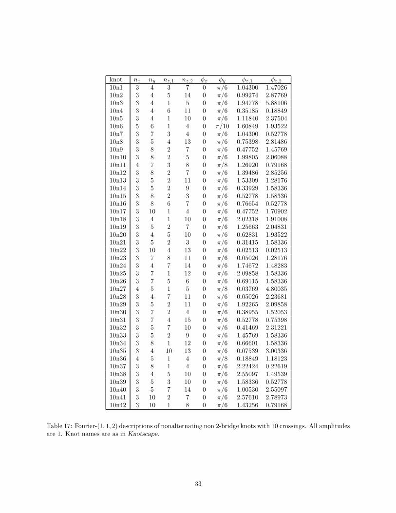
We made only a modest attempt to sample Fourier-(1, 1, 2) knots with x and y frequencies greater than two.Rather than sampling at random as in Section 5.3, we now chose one sampling point from each region of thephase torus by first creating a bitmap image as in Figure 3 and then taking the centroid of each white region.Sometimes the centroid fell outside of the region and in this case an arbitrary point of the region was selected.Because of the large crossing numbers that result, and the consequent difficulty in identifying these knots,we again restricted our sample to x and y frequencies of (3, 4), (3, 5), (3, 7), (3, 8), (3, 10), (4, 5), (4, 7) or (5, 6).We further restricted the z-frequencies to be less than 15 and somewhat arbitrarily fixed all amplitudes at1. Using Knotscape to identify the resulting knots, and keeping only knots with 16 or less crossings, wefound several thousand prime knots. In Tables 14–16 we list all of these with 10 or less crossings whichare not 2-bridge and thus listed in Tables 12–13. All knots through 9 crossings were found, and all but 20alternating 10-crossings knots were found. We suspect that limiting the z-frequencies to less than 15 is asevere restriction.

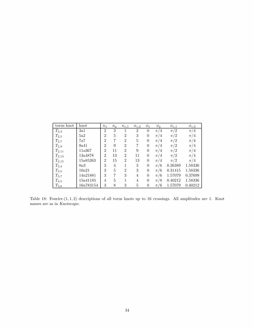
We did however, find all torus knots up to 16 crossings. It is shown by Kauffman in [9] that every torusknot is a Fourier-(1, 3, 3) knot. Interestingly, we found that, up to 16 crossings, the torus knot Tp,q canbe represented by a Fourier-(1, 1, 2) knot with nx = p and ny = q. Table 18 lists these results. The datasuggests the following conjectures (which we have verified for a large number of (p, q) pairs, and hope toprove in a later paper).

Conjecture 13. The torus knot T2,q can be represented as a Fourier-(1, 1, 2) knot with frequencies nx =2, ny = q, nz,1 = 2 and nz,2 = q − 2 and phase shifts φx = 0, φy = π/4, φz,1 = π/2 and φz,2 = π/4.

18

Conjecture 14. The torus knot Tp,q, with 0 < p < q, can be represented as a Fourier-(1, 1, 2) knot withfrequencies nx = p, ny = q, nz,1 = p and nz,2 = q − p.

It would be interesting to undertake a large-scale sampling of Fourier-(1, 1, 2) knots with x and y frequenciesgreater than two to see if every knot with 16 or less crossings turns up. Such a study might shed light onthe following question,

Question 4. Is there a knot which cannot be expressed as a Fourier-(1, 1, k) knot for k ≤ 2?

References

[1] M. G. V. Bogle, J. E. Hearst, V. F. R. Jones, and L. Stoilov. Lissajous knots. J. Knot TheoryRamifications, 3(2):121–140, 1994.

[2] Gerhard Burde and Heiner Zieschang. Knots, volume 5 of de Gruyter Studies in Mathematics. Walterde Gruyter & Co., Berlin, 2003.

[3] Peter Cromwell. Knots and Links. Cambridge University Press, 2004.

[4] Richard Hartley and Akio Kawauchi. Polynomials of amphicheiral knots. Math. Ann., 243(1):63–70,1979.

[5] Jim Hoste and Morwen Thistlethwaite. Knotscape. http://www.math.utk.edu/∼morwen, 1998.

[6] Jim Hoste, Morwen Thistlethwaite, and Jeff Weeks. The first 1,701,936 knots. Math. Intelligencer,20(4):33–48, 1998.

[7] Jim Hoste and Laura Zirbel. Lissajous knots with lissajous projections. arXiv: math.GT/0605632,2006.

[8] Vaughan F. R. Jones and Jozef H. Przytycki. Lissajous knots and and billiard knots. Banach CenterPublications, (42):145–163, 1998.

[9] Louis H. Kauffman. Fourier Knots. arXiv: q-alg/9711013

[10] Christoph Lamm. Fourier knots. Preprint.

[11] Christoph Lamm. There are infinitely many lissajous knots. Manuscripta Math., 93:29–37, 1996.

[12] Kunio Murasugi. On periodic knots. Comment. Math. Helv., 46:162–174, 1971.

[13] Jozef Przytycki. Symmetric knots and billiard knots. arXiv: math.GT/0405151

[14] Dale Rolfsen. Knots and links, volume 7 of Mathematics Lecture Series. Publish or Perish Inc., Houston,TX, 1990. Corrected reprint of the 1976 original.

19

6 Tables of Lissajous and Fourier Knots

L(2, 3) L(2, 5) L(2, 7) L(2, 9) L(2, 11) L(2, 13) L(2, 15)cr p/q p/q p/q p/q p/q p/q p/q5 7/2 7/2 7/2 7/2 7/2 7/2 7/26 9/2 9/2 9/2 9/2 9/2 9/2 9/27 15/4 17/5 15/4 17/5 15/4 15/4 17/57 17/5 17/5 17/58 31/129 15/2 31/7 15/2 15/2 15/29 31/7 31/7 31/7 31/79 31/1110 17/2 17/2 17/2 55/12 17/2 55/1210 49/20 49/20 57/16 57/16 49/20 57/1610 57/16 55/12 57/1610 57/1611 65/14 73/16 49/9 49/9 41/13 49/911 73/16 65/14 73/16 49/9 73/1611 97/26 73/16 71/2011 73/1611 97/2612 121/32 169/50 167/46 121/32 167/46 169/5012 169/5013 209/56 239/71 23/2 71/11 23/213 71/11 209/56 71/1114 25/2 25/2 407/119 25/2 407/11914 89/36 89/36 409/12114 289/118 289/11814 409/12115 151/20 441/101 151/20 97/13 97/1315 319/144 463/130 319/144 361/78 463/13015 359/82 359/82 463/13015 463/130 433/12215 447/9815 463/13016 529/114 593/130 593/130 529/114 593/13016 593/130 817/239 559/122 817/23916 777/208 593/13016 815/23717 975/274 703/131 1353/380 31/217 983/260 1321/288 127/1517 1351/362 975/27417 983/260

Table 4: The sets L(2, ny) for 3 ≤ ny ≤ 15 given by crossing number and 2-bridge fraction p/q.

20

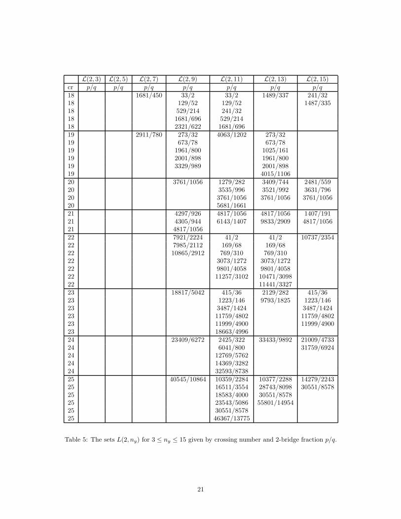
L(2, 3) L(2, 5) L(2, 7) L(2, 9) L(2, 11) L(2, 13) L(2, 15)cr p/q p/q p/q p/q p/q p/q p/q18 1681/450 33/2 33/2 1489/337 241/3218 129/52 129/52 1487/33518 529/214 241/3218 1681/696 529/21418 2321/622 1681/69619 2911/780 273/32 4063/1202 273/3219 673/78 673/7819 1961/800 1025/16119 2001/898 1961/80019 3329/989 2001/89819 4015/110620 3761/1056 1279/282 3409/744 2481/55920 3535/996 3521/992 3631/79620 3761/1056 3761/1056 3761/105620 5681/166121 4297/926 4817/1056 4817/1056 1407/19121 4305/944 6143/1407 9833/2909 4817/105621 4817/105622 7921/2224 41/2 41/2 10737/235422 7985/2112 169/68 169/6822 10865/2912 769/310 769/31022 3073/1272 3073/127222 9801/4058 9801/405822 11257/3102 10471/309822 11441/332723 18817/5042 415/36 2129/282 415/3623 1223/146 9793/1825 1223/14623 3487/1424 3487/142423 11759/4802 11759/480223 11999/4900 11999/490023 18663/499624 23409/6272 2425/322 33433/9892 21009/473324 6041/800 31759/692424 12769/576224 14369/328224 32593/873825 40545/10864 10359/2284 10377/2288 14279/224325 16511/3554 28743/8098 30551/857825 18583/4000 30551/857825 23543/5086 55801/1495425 30551/857825 46367/13775

Table 5: The sets L(2, ny) for 3 ≤ ny ≤ 15 given by crossing number and 2-bridge fraction p/q.

21

L(2, 3) L(2, 5) L(2, 7) L(2, 9) L(2, 11) L(2, 13) L(2, 15)cr p/q p/q p/q p/q p/q p/q p/q26 34905/7522 49/2 49/226 34969/7666 209/84 209/8426 39129/8578 1009/406 1009/40626 51193/14384 4465/1848 4465/184826 17921/7418 17921/741826 39129/8578 39129/857826 57121/23660 57121/2366026 80305/23857 97681/2889827 64343/18066 601/48 3871/51427 64351/18068 1793/14227 64863/17156 6409/259227 87031/23298 21401/873827 69121/2822227 69361/2832027 85561/1959727 91193/2558428 108241/28622 4385/514 162521/4827928 108657/28732 10817/126828 151313/40544 26937/312228 78489/3202028 80089/3594028 151697/4488229 188175/50374 21441/2840 136399/2541929 188287/50404 50969/1164229 262087/70226 81025/3657629 91193/2083029 115561/2639629 259969/6967630 326041/87362 84041/18530 57/230 134689/28992 249/10030 151553/32622 1249/50230 191561/41968 5857/242430 248169/69680 26041/1077830 453929/121630 104441/4326030 248169/6968030 332929/13790230 448689/120112

Table 6: The sets L(2, ny) for 3 ≤ ny ≤ 15 given by crossing number and 2-bridge fraction p/q.

22

L(2, 3) L(2, 5) L(2, 7) L(2, 9) L(2, 11) L(2, 13) L(2, 15)cr p/q p/q p/q p/q p/q p/q p/q31 564719/151316 283537/61102 807/5231 284049/62270 2599/21031 284057/62272 9215/372831 317849/69680 39159/1584231 415929/116866 127399/5154031 645809/191861 317849/6968031 400895/16646431 402287/16425832 522665/146752 1118489/33226132 522729/14676832 526889/13936032 697745/18678433 864945/228716 38951/517233 872153/230622 97015/1288233 882809/233440 241791/3202033 1216977/326170 511079/23062433 511119/23064233 575119/13136233 1191711/27295134 1509537/404098 2090425/55960234 1515361/40746034 2107561/56472035 2621905/702714 2015903/56601835 2622017/70252035 3650401/97812236 4541161/1216800 2303201/49633836 2307361/50582636 2307425/50584236 2581921/56601836 6322681/169416237 7865521/2107560 4245663/119208237 4246175/119222637 4246183/119221237 4279975/113203637 8994959/267227938 9748249/260958440 21077281/564233840 21089825/564569840 29354521/786552041 50843527/1362348242 63250209/1694784243 109552575/29354524

Table 7: The sets L(2, ny) for 3 ≤ ny ≤ 15 given by crossing number and 2-bridge fraction p/q.

23

knot p/q nx ny nz φx φy φz

5a1 7/2 2 3 11 0 0.56099 2.580596a3 9/2 2 3 11 0 0.67319 0.897597a3 17/5 2 5 17 0 0.49979 2.641797a6 15/4 2 3 11 0 0.78539 2.356198a1 31/12 2 11 41 0 0.39269 2.748899a8 31/11 2 11 41 0 0.48332 1.087479a27 15/2 2 7 25 0 0.49087 1.079929a33 31/7 2 7 23 0 0.47123 2.6703510a23 49/20 2 5 17 0 0.71399 0.8567910a63 55/12 2 7 25 0 0.44178 2.6998010a69 57/16 2 5 19 0 0.58904 2.5525410a75 17/2 2 5 17 0 0.57119 0.9995911a91 129/49 2 41 153 0 0.34816 2.7934211a140 65/17 2 17 63 0 0.47123 1.0995511a192 97/26 2 5 17 0 0.64259 2.4989911a210 73/16 2 5 19 0 0.65449 0.9162911a226 71/20 2 13 49 0 0.45603 1.1147511a246 41/13 2 13 47 0 0.47123 1.0995511a333 65/14 2 5 19 0 0.78539 0.7853911a334 49/9 2 9 29 0 0.45470 2.6868812a38 71/28 2 25 89 0 0.41336 1.1574212a257 191/74 2 17 63 0 0.37306 2.7685212a715 169/50 2 7 25 0 0.53996 2.6016312a729 167/46 2 9 31 0 0.43196 2.7096212a1034 121/32 2 5 19 0 0.71994 2.4216413a640 55/19 2 19 65 0 0.44879 1.1219913a1884 289/80 2 25 93 0 0.35941 2.7821713a2683 287/79 2 63 235 0 0.34262 2.7989613a2760 239/71 2 7 23 0 0.57595 2.5656313a3143 23/2 2 11 37 0 0.45814 1.1126413a3896 111/23 2 23 85 0 0.46542 1.1053713a4304 209/56 2 5 17 0 0.78539 2.3561913a4570 79/19 2 19 69 0 0.46409 1.1066913a4822 71/11 2 11 35 0 0.44392 2.69767

Table 8: All Lissajous knots with frequencies nx = 2, 3 ≤ ny ≤ 105 and with less than 14 crossings. Knotnames are as in Knotscape.

24

knot p/q nx ny nz φx φy φz

14a2651 89/36 2 7 23 0 0.62831 0.9424714a6166 289/118 2 7 23 0 0.73303 0.8377514a12186 407/119 2 11 37 0 0.42542 2.7161614a12212 409/121 2 9 31 0 0.51050 2.6310814a12308 103/12 2 57 215 0 0.36382 2.7777614a12652 127/28 2 29 103 0 0.40459 1.1661914a12741 25/2 2 7 23 0 0.52359 1.0471915a21965 113/29 2 29 99 0 0.44178 1.1290015a25723 745/288 2 19 71 0 0.40142 2.7401615a32142 319/144 2 7 25 0 0.78539 0.7853915a44612 359/82 2 7 25 0 0.68722 0.8835715a46260 361/78 2 13 49 0 0.50670 1.0640815a50643 447/98 2 11 39 0 0.40840 2.7331815a50772 433/122 2 11 41 0 0.45311 2.6884715a51438 463/130 2 7 27 0 0.60059 2.5409915a52567 151/20 2 7 25 0 0.58904 0.9817415a54893 65/21 2 21 71 0 0.44392 1.1268715a71359 505/109 2 85 317 0 0.33994 2.8016415a71603 169/29 2 29 107 0 0.46199 1.1087915a76044 441/101 2 9 29 0 0.53737 2.6042115a78853 129/25 2 25 91 0 0.46040 1.1103915a84772 97/13 2 13 41 0 0.43633 2.7052616a7016 111/44 2 39 131 0 0.40655 1.1642316a57423 431/170 2 39 139 0 0.40593 1.1648616a135506 1103/456 2 23 85 0 0.36361 2.7779816a219884 961/208 2 93 347 0 0.33914 2.8024416a221291 777/208 2 7 25 0 0.63813 2.5034516a221836 783/220 2 41 155 0 0.37667 2.7649216a224238 791/212 2 17 65 0 0.44058 2.7010016a225074 593/130 2 7 27 0 0.64679 0.9239916a228722 559/122 2 13 47 0 0.39269 2.7488916a229409 577/162 2 21 79 0 0.43982 1.1309716a249132 817/239 2 11 37 0 0.49087 2.6507116a249195 815/237 2 13 43 0 0.42074 2.7208416a252419 385/114 2 43 153 0 0.40071 1.1700816a252465 399/110 2 47 177 0 0.37166 2.7699316a333209 529/114 2 7 27 0 0.73919 0.83159

Table 9: All Lissajous knots with frequencies nx = 2, 3 ≤ ny ≤ 105 and with 14–16 crossings. Knot namesare as in Knotscape.

25

knot nx ny nz φx φy φz

5a1 3 4 29 0 0.49186 1.602526a3 3 4 29 0 0.39666 1.697727a6 3 7 68 0 0.52359 2.617998a2 3 4 23 0 0.29088 2.850708n2 3 4 37 0 0.49805 2.643539a25 3 5 28 0 0.26973 1.8246610a20 3 4 23 0 0.32967 0.7175210a73 3 7 40 0 0.23394 2.9076410a89 3 4 29 0 0.36493 0.6822610a103 3 5 29 0 0.41579 2.7257910n28 3 7 40 0 0.21166 1.8827211n50 4 5 57 0 0.36736 1.9888311n151 4 7 69 0 0.24802 1.3227712a426 3 10 83 0 0.45603 2.6855512a427 3 5 29 0 0.32339 2.8181912a448 3 5 28 0 0.30146 0.7457312a868 3 5 26 0 0.28713 1.8072612a1164 4 5 61 0 0.34509 2.0110912n133 3 4 23 0 0.36845 1.7259312n293 3 10 59 0 0.28077 1.8136212n322 4 5 37 0 0.16829 2.1878912n483 5 6 113 0 0.35111 2.1621513a2233 3 8 67 0 0.48171 2.6598813a4774 3 4 23 0 0.40724 2.7343413n1405 4 5 51 0 0.35062 2.0055713n1734 3 10 103 0 0.56066 1.5337213n3594 3 4 23 0 0.44602 0.60116

Table 10: Small-crossing Lissajous knots with all frequencies greater than 2. Only three knots, 5a1, 6a3 and7a6 are 2-bridge and appear in Table 8. Knot names are as in Knotscape.

26

knot nx ny nz φx φy φz

14a1491 4 5 39 0 0.19634 0.5890414a6398 3 7 59 0 0.49979 2.6417914a6912 3 8 67 0 0.42586 0.6213314a8662 3 7 53 0 0.35779 0.6894014a13089 4 7 53 0 0.15707 1.4137114a15296 3 4 29 0 0.46013 0.5870614a16309 3 7 53 0 0.47996 1.6144214a16437 3 5 29 0 0.35419 1.7401914a18187 3 5 37 0 0.38646 0.6607314n6560 3 8 47 0 0.25703 2.8845514n9732 3 7 53 0 0.42760 1.6667814n13886 3 4 29 0 0.42839 2.7131914n14189 4 5 63 0 0.39269 2.7488914n15552 3 5 28 0 0.33319 2.8083914n18513 3 8 83 0 0.58113 1.5132514n22071 3 7 64 0 0.50884 2.6327414n22073 3 5 29 0 0.50819 2.6333914n23738 3 7 50 0 0.39499 1.6993914n24494 3 8 61 0 0.35665 1.7377414n25903 3 7 53 0 0.37524 1.7191415a80928 4 5 37 0 0.20569 0.5796915n77228 4 5 69 0 0.42453 1.1462515n92508 3 8 61 0 0.43253 2.7090515n103019 5 6 103 0 0.30263 2.8389615n116110 4 7 53 0 0.14398 2.2122016a128851 3 7 40 0 0.30079 2.8408016a151023 3 7 38 0 0.26761 0.7795816a168328 3 7 41 0 0.29452 2.8470616a202258 3 7 40 0 0.27850 1.8158816a295212 3 5 26 0 0.38847 1.7059116a312423 3 5 29 0 0.38499 0.6621916a340770 3 7 41 0 0.38179 0.6654016n42863 4 5 39 0 0.21419 1.3565916n228473 3 7 38 0 0.29088 1.8035016n390014 3 5 26 0 0.35469 2.7868916n507235 3 5 28 0 0.39666 0.6505316n562396 3 5 28 0 0.36493 1.7294616n768985 3 4 23 0 0.48481 1.6095816n982564 4 5 73 0 0.44304 1.1277516n988939 3 7 41 0 0.51269 0.5345016n1008347 3 7 50 0 0.32150 0.72568

Table 11: Small-crossing Lissajous knots with all frequencies greater than 2. Knot names are as in Knotscape.

27

knot p/q nx ny nz,1 nz,2 φx φy φz,1 φz,2

3a1 3/1 2 3 1 2 0 π/4 0.39269 1.660174a1 5/2 2 3 1 3 0 π/4 1.62773 5.792545a1 7/2 2 3 1 7 0 π/4 0.10580 2.493205a2 5/1 2 5 2 3 0 π/4 0.96046 4.097676a1 13/5 2 5 1 5 0 π/4 0.03573 2.533536a2 11/3 2 7 1 7 0 π/4 1.90655 5.016376a3 9/2 2 3 1 5 0 π/4 0.18165 1.759457a1 21/8 2 5 1 5 0 π/4 1.60021 5.524127a2 19/7 2 7 3 7 0 π/4 1.66835 6.112717a3 17/5 2 7 5 9 0 π/4 0.08774 5.557457a4 11/2 2 7 3 7 0 π/4 1.60853 6.273847a5 13/3 2 9 4 7 0 π/4 1.57817 4.410327a6 15/4 2 3 1 7 0 π/4 1.87792 4.643527a7 7/1 2 7 2 5 0 π/4 0.93991 0.931048a1 31/12 2 11 1 5 0 π/4 0.37204 1.787958a4 25/9 2 7 1 5 0 π/4 2.04720 5.291978a5 29/12 2 5 3 5 0 π/4 1.59453 2.058218a6 23/5 2 9 1 9 0 π/4 0.35397 2.657108a7 29/8 2 9 1 5 0 π/4 1.47451 2.104478a8 17/3 2 11 3 10 0 π/4 0.39241 5.091828a9 27/8 2 9 1 5 0 π/4 2.03830 2.056688a10 23/7 2 7 1 9 0 π/4 0.48400 5.189158a11 13/2 2 5 3 5 0 π/4 1.58524 0.245318a16 25/7 2 7 3 7 0 π/4 0.04412 2.252488a17 19/4 2 9 3 7 0 π/4 1.92077 6.064578a18 17/4 2 7 1 5 0 π/4 1.42912 1.987979a3 41/16 2 7 3 5 0 π/4 1.88608 4.988549a8 31/11 2 5 7 9 0 π/4 0.09293 5.505169a10 39/16 2 5 1 7 0 π/4 2.08636 5.173679a12 49/18 2 17 1 9 0 π/4 0.60289 4.563329a13 55/21 2 7 1 7 0 π/4 0.00613 5.431349a14 39/14 2 9 1 9 0 π/4 2.13083 5.890359a15 47/13 2 9 1 9 0 π/4 1.74912 1.923229a16 45/19 2 9 1 5 0 π/4 1.93719 4.943289a17 37/8 2 5 2 9 0 π/4 0.19367 2.962959a19 41/11 2 15 3 10 0 π/4 2.62089 0.608449a20 33/7 2 17 5 7 0 π/4 0.10752 5.130869a21 43/12 2 5 3 9 0 π/4 2.14045 5.612059a22 35/8 2 5 7 9 0 π/4 1.67486 1.659799a23 27/5 2 13 4 5 0 π/4 1.36285 5.388819a24 41/12 2 11 1 7 0 π/4 0.44828 2.243399a26 29/9 2 11 8 9 0 π/4 1.42268 3.500989a27 15/2 2 5 1 7 0 π/4 0.00135 6.211849a33 31/7 2 11 4 9 0 π/4 0.93417 3.860389a34 37/10 2 9 3 5 0 π/4 1.98367 5.566189a35 21/4 2 11 9 10 0 π/4 0.35932 5.183059a36 23/4 2 9 3 5 0 π/4 1.65102 3.045939a38 19/3 2 13 1 7 0 π/4 1.93386 2.029109a39 33/10 2 11 3 7 0 π/4 2.16159 2.032139a41 9/1 2 9 2 7 0 π/4 0.86114 0.74621

Table 12: Fourier-(1, 1, 2) descriptions of all 2-bridge knots to 9 crossings. All amplitudes are 1. Boldfaceentries are known to be Lissajous while italic entries might be Lissajous. All others cannot be Lissajous.Knot names are as in Knotscape.

28

knot p/q nx ny nz,1 nz,2 φx φy φz,1 φz,2

10a5 51/20 2 11 3 7 0 π/4 0.18595 2.8247010a19 37/13 2 13 3 7 0 π/4 1.85642 1.8338610a23 49/20 2 5 1 7 0 π/4 0.36657 2.4728110a25 89/34 2 7 1 7 0 π/4 1.62228 5.5977510a26 61/22 2 17 3 8 0 π/4 0.19982 4.4338710a29 59/25 2 9 1 5 0 π/4 1.82942 5.2982810a30 75/29 2 15 5 7 0 π/4 1.66311 4.7925010a31 81/31 2 17 3 7 0 π/4 1.36514 5.0745710a32 79/29 2 17 3 7 0 π/4 2.51922 6.1003210a33 57/13 2 17 1 9 0 π/4 1.22778 5.4869810a34 67/18 2 13 1 5 0 π/4 1.94658 5.2099610a35 71/26 2 17 5 7 0 π/4 2.17223 4.4644210a43 47/11 2 17 5 8 0 π/4 2.17425 5.5021110a44 53/14 2 9 3 5 0 π/4 2.12967 5.3983210a49 53/23 2 13 1 7 0 π/4 1.00888 3.5744610a52 73/27 2 17 3 7 0 π/4 2.90021 2.8012110a53 63/17 2 17 1 9 0 π/4 0.46162 2.9108210a54 53/12 2 5 5 7 0 π/4 0.00438 1.9651810a55 69/19 2 13 3 7 0 π/4 2.09996 5.2316510a56 33/5 2 19 5 6 0 π/4 0.37923 4.7223910a57 59/18 2 21 3 8 0 π/4 0.38316 4.4811710a58 71/21 2 13 6 9 0 π/4 1.04484 0.6434310a59 23/3 2 23 2 7 0 π/4 0.57078 0.1028010a60 45/14 2 17 1 9 0 π/4 1.72208 1.8114410a61 65/19 2 17 2 5 0 π/4 1.05935 4.5312810a63 55/12 2 11 1 7 0 π/4 2.07884 1.8094210a64 45/8 2 17 5 9 0 π/4 1.41312 1.4989210a65 43/8 2 19 1 7 0 π/4 1.64470 4.0325610a68 43/9 2 13 9 10 0 π/4 0.30693 1.3100710a69 57/16 2 9 3 5 0 π/4 0.02223 2.4617310a70 37/7 2 19 5 7 0 π/4 0.36129 4.6928710a71 55/16 2 13 3 5 0 π/4 1.15846 5.7155810a74 35/11 2 13 5 10 0 π/4 0.31052 4.1815710a75 17/2 2 5 2 7 0 π/4 0.00295 3.1066910a107 41/9 2 9 5 9 0 π/4 0.11322 5.4449610a108 51/11 2 17 2 7 0 π/4 1.01343 4.4987810a109 65/18 2 11 2 5 0 π/4 0.22667 5.3092510a110 39/7 2 19 4 5 0 π/4 1.10277 4.4269110a111 61/17 2 19 4 5 0 π/4 1.35067 1.2308810a112 49/13 2 17 5 7 0 π/4 0.06896 1.2408610a113 27/4 2 17 4 7 0 π/4 1.05187 2.2038010a114 29/5 2 19 5 7 0 π/4 0.18690 4.4516710a115 47/10 2 11 7 10 0 π/4 0.50632 4.5321610a116 43/10 2 15 7 9 0 π/4 0.09320 1.9401310a117 25/4 2 7 1 5 0 π/4 2.15907 2.20357

Table 13: Fourier-(1, 1, 2) descriptions of all 2-bridge knots with 10 crossings. All amplitudes are 1. Boldfaceentries are known to be Lissajous while italic entries might be Lissajous. All others cannot be Lissajous.Knot names are as in Knotscape.

29

knot nx ny nz,1 nz,2 φx φy φz,1 φz,2

8a2 3 4 1 7 0 π/6 1.63362 2.035758a3 3 5 6 13 0 π/6 0.56548 2.035758a12 3 4 3 5 0 π/6 1.04300 0.804248a13 3 4 1 9 0 π/6 0.26389 1.583368a14 3 4 7 14 0 π/6 1.28176 1.784428a15 3 7 1 10 0 π/6 1.64619 2.312218n1 3 4 1 14 0 π/6 1.94778 2.764608n2 3 4 1 5 0 π/6 0.05026 2.236818n3 3 4 1 3 0 π/6 0.26389 1.583369a1 3 5 7 10 0 π/6 2.29964 0.037699a2 3 7 1 6 0 π/6 0.35185 1.055579a4 3 4 1 14 0 π/6 1.33203 2.274519a5 3 8 1 8 0 π/6 0.65345 1.709029a6 3 7 1 10 0 π/6 1.88495 2.437879a7 3 4 1 14 0 π/6 2.03575 2.375049a9 3 7 4 15 0 π/6 1.15610 0.766549a11 3 5 9 14 0 π/6 1.04300 1.332039a18 3 4 2 7 0 π/6 2.37504 2.035759a25 3 7 2 14 0 π/6 0.98017 0.376999a28 3 7 4 5 0 π/6 1.28176 0.452389a29 4 7 2 13 0 π/8 0.26389 2.073459a30 3 7 8 9 0 π/6 0.23876 0.779119a31 3 4 10 11 0 π/6 1.38230 1.872389a32 3 7 4 13 0 π/6 0.46495 1.206379a37 3 4 2 11 0 π/6 1.04300 2.626379a40 3 7 4 13 0 π/6 1.06814 1.068149n1 3 4 1 14 0 π/6 0.05026 0.276469n2 3 5 4 7 0 π/6 0.15079 1.998059n3 3 8 1 6 0 π/6 0.76654 0.955049n4 3 4 2 11 0 π/6 0.35185 2.513279n5 3 4 1 4 0 π/6 1.33203 2.098589n6 3 4 2 13 0 π/6 0.08796 2.488149n7 3 7 2 9 0 π/6 2.62637 1.055579n8 3 7 4 13 0 π/6 0.05026 0.18849

Table 14: Fourier-(1, 1, 2) descriptions of non 2-bridge knots up to 9 crossings. All amplitudes are 1. Knotnames are as in Knotscape.

30

knot nx ny nz,1 nz,2 φx φy φz,1 φz,2

10a1 3 4 5 9 0 π/6 1.04300 1.5833610a2 3 8 4 13 0 π/6 0.70371 0.0879610a3 3 8 7 14 0 π/6 2.70176 0.2387610a4 3 5 4 13 0 π/6 2.34991 2.3499110a7 3 5 8 11 0 π/6 0.01256 1.6084910a9 3 8 5 6 0 π/6 0.27646 1.5833610a10 3 10 2 11 0 π/6 2.48814 2.9405310a11 3 8 3 14 0 π/6 0.05026 1.0178710a12 3 8 2 5 0 π/6 1.40743 1.6713210a14 3 8 2 7 0 π/6 0.33929 2.8148610a15 4 7 1 12 0 π/8 1.01787 0.6785810a16 4 7 1 12 0 π/8 0.20106 0.6660110a17 3 8 5 15 0 π/6 0.22619 1.0681410a18 3 8 4 9 0 π/6 0.17592 1.5833610a20 3 4 1 7 0 π/6 0.22619 1.4702610a21 3 8 1 10 0 π/6 0.82938 2.7143310a22 3 8 1 10 0 π/6 2.46300 2.7520310a28 4 7 1 14 0 π/8 0.43982 0.1130910a36 4 5 1 14 0 π/8 0.82938 1.6084910a37 3 5 7 14 0 π/6 0.07539 2.9028310a38 3 7 2 11 0 π/6 0.66601 0.0125610a42 3 10 5 8 0 π/6 2.61380 0.4272510a47 3 4 5 14 0 π/6 2.19911 1.9603510a48 3 8 5 10 0 π/6 2.02318 1.3948610a50 3 7 1 8 0 π/6 1.60849 1.0932710a51 3 7 2 4 0 π/6 2.56353 5.4538010a62 5 6 4 11 0 π/10 0.27646 0.5906110a66 3 5 2 11 0 π/6 1.52053 1.8598210a67 3 8 2 13 0 π/6 1.40743 3.12902

Table 15: Fourier-(1, 1, 2) descriptions of alternating non 2-bridge knots with 10 crossings. All amplitudesare 1. Knot names are as in Knotscape.

31

knot nx ny nz,1 nz,2 φx φy φz,1 φz,2

10a72 4 5 7 14 0 π/8 2.47557 1.7341510a73 3 5 2 10 0 π/6 1.98548 0.1633610a76 3 7 6 11 0 π/6 1.58336 1.0555710a77 5 6 3 14 0 π/10 0.30159 1.7592910a78 5 6 1 12 0 π/10 1.45769 1.2692010a80 3 10 4 15 0 π/6 1.97292 0.3141510a82 5 6 4 11 0 π/10 0.37699 2.8651310a84 4 7 6 13 0 π/8 0.31415 1.7341510a85 3 4 7 14 0 π/6 1.08070 2.0483110a87 4 7 2 3 0 π/8 1.43256 2.1488410a89 3 4 3 13 0 π/6 0.18849 1.4828310a90 5 6 6 7 0 π/10 0.02513 1.5330910a91 4 7 1 14 0 π/8 0.70371 0.0502610a92 3 4 7 14 0 π/6 1.09327 2.4630010a93 3 8 2 13 0 π/6 1.57079 0.6911510a94 3 4 7 10 0 π/6 1.28176 1.3697310a95 4 7 4 13 0 π/8 1.58336 0.0628310a96 3 4 7 13 0 π/6 1.63362 5.1773410a97 3 8 2 7 0 π/6 1.35716 2.3624710a99 3 8 2 7 0 π/6 1.36973 2.6389310a100 3 10 4 7 0 π/6 1.73415 1.4199910a101 5 6 3 8 0 π/10 0.06283 2.5761010a102 3 4 1 13 0 π/6 2.02318 1.2440710a103 3 5 9 13 0 π/6 0.75398 2.5761010a105 3 4 10 13 0 π/6 1.77185 2.8651310a119 4 7 10 15 0 π/8 0.45238 1.2566310a121 3 5 3 7 0 π/6 1.04300 0.8545110a122 4 7 7 9 0 π/8 1.28176 3.9961010a123 3 7 2 6 0 π/6 0.57805 4.31026

Table 16: Fourier-(1, 1, 2) descriptions of alternating non 2-bridge knots with 10 crossings. All amplitudesare 1. Knot names are as in Knotscape.

32

knot nx ny nz,1 nz,2 φx φy φz,1 φz,2

10n1 3 4 3 7 0 π/6 1.04300 1.4702610n2 3 4 5 14 0 π/6 0.99274 2.8776910n3 3 4 1 5 0 π/6 1.94778 5.8810610n4 3 4 6 11 0 π/6 0.35185 0.1884910n5 3 4 1 10 0 π/6 1.11840 2.3750410n6 5 6 1 4 0 π/10 1.60849 1.9352210n7 3 7 3 4 0 π/6 1.04300 0.5277810n8 3 5 4 13 0 π/6 0.75398 2.8148610n9 3 8 2 7 0 π/6 0.47752 1.4576910n10 3 8 2 5 0 π/6 1.99805 2.0608810n11 4 7 3 8 0 π/8 1.26920 0.7916810n12 3 8 2 7 0 π/6 1.39486 2.8525610n13 3 5 2 11 0 π/6 1.53309 1.2817610n14 3 5 2 9 0 π/6 0.33929 1.5833610n15 3 8 2 3 0 π/6 0.52778 1.5833610n16 3 8 6 7 0 π/6 0.76654 0.5277810n17 3 10 1 4 0 π/6 0.47752 1.7090210n18 3 4 1 10 0 π/6 2.02318 1.9100810n19 3 5 2 7 0 π/6 1.25663 2.0483110n20 3 4 5 10 0 π/6 0.62831 1.9352210n21 3 5 2 3 0 π/6 0.31415 1.5833610n22 3 10 4 13 0 π/6 0.02513 0.0251310n23 3 7 8 11 0 π/6 0.05026 1.2817610n24 3 4 7 14 0 π/6 1.74672 1.4828310n25 3 7 1 12 0 π/6 2.09858 1.5833610n26 3 7 5 6 0 π/6 0.69115 1.5833610n27 4 5 1 5 0 π/8 0.03769 4.8003510n28 3 4 7 11 0 π/6 0.05026 2.2368110n29 3 5 2 11 0 π/6 1.92265 2.0985810n30 3 7 2 4 0 π/6 0.38955 1.5205310n31 3 7 4 15 0 π/6 0.52778 0.7539810n32 3 5 7 10 0 π/6 0.41469 2.3122110n33 3 5 2 9 0 π/6 1.45769 1.5833610n34 3 8 1 12 0 π/6 0.66601 1.5833610n35 3 4 10 13 0 π/6 0.07539 3.0033610n36 4 5 1 4 0 π/8 0.18849 1.1812310n37 3 8 1 4 0 π/6 2.22424 0.2261910n38 3 4 5 10 0 π/6 2.55097 1.4953910n39 3 5 3 10 0 π/6 1.58336 0.5277810n40 3 5 7 14 0 π/6 1.00530 2.5509710n41 3 10 2 7 0 π/6 2.57610 2.7897310n42 3 10 1 8 0 π/6 1.43256 0.79168

Table 17: Fourier-(1, 1, 2) descriptions of nonalternating non 2-bridge knots with 10 crossings. All amplitudesare 1. Knot names are as in Knotscape.

33

torus knot knot nx ny nz,1 nz,2 φx φy φz,1 φz,2

T2,3 3a1 2 3 1 2 0 π/4 π/2 π/4T2,5 5a2 2 5 2 3 0 π/4 π/2 π/4T2,7 7a7 2 7 2 5 0 π/4 π/2 π/4T2,9 9a41 2 9 2 7 0 π/4 π/2 π/4T2,11 11a367 2 11 2 9 0 π/4 π/2 π/4T2,13 13a4878 2 13 2 11 0 π/4 π/2 π/4T2,15 15a85263 2 15 2 13 0 π/4 π/2 π/4T3,4 8n3 3 4 1 3 0 π/6 0.26389 1.58336T3,5 10n21 3 5 2 3 0 π/6 0.31415 1.58336T3,7 14n21881 3 7 3 4 0 π/6 1.57079 0.37699T4,5 15n41185 4 5 1 4 0 π/8 0.40212 1.58336T3,8 16n783154 3 8 3 5 0 π/6 1.57079 0.40212

Table 18: Fourier-(1, 1, 2) descriptions of all torus knots up to 16 crossings. All amplitudes are 1. Knotnames are as in Knotscape.

34