Rigid Body Dynamics (I)

COMP259 March 28, 2006Nico Galoppo von Borries

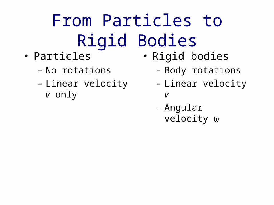
From Particles to Rigid Bodies

• Particles– No rotations– Linear velocity v

only

• Rigid bodies– Body rotations– Linear velocity v– Angular velocity ω

Outline

• Rigid Body Preliminaries– Coordinate system, velocity,

acceleration, and inertia• State and Evolution• Quaternions• Collision Detection and Contact

Determination• Colliding Contact Response

Coordinate Systems

• Body Space (Local Coordinate System)– bodies are specified relative to this

system– center of mass is the origin (for

convenience)•We will specify body-related physical

properties (inertia, …) in this frame

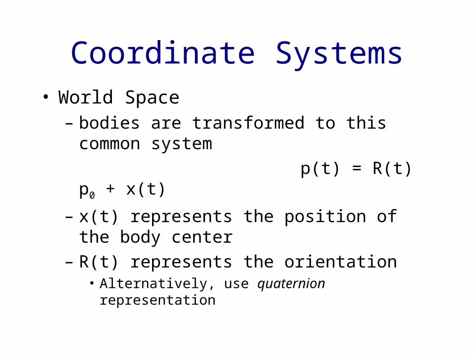
Coordinate Systems• World Space

– bodies are transformed to this common system

p(t) = R(t) p0 + x(t)

– x(t) represents the position of the body center

– R(t) represents the orientation• Alternatively, use quaternion representation

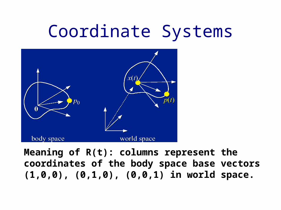
Coordinate Systems

Meaning of R(t): columns represent the coordinates of the body space base vectors (1,0,0), (0,1,0), (0,0,1) in world space.

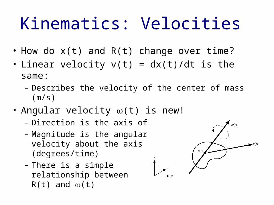
Kinematics: Velocities

• How do x(t) and R(t) change over time?• Linear velocity v(t) = dx(t)/dt is the same:

– Describes the velocity of the center of mass (m/s)

• Angular velocity (t) is new!– Direction is the axis of rotation– Magnitude is the angular

velocity about the axis (degrees/time)

– There is a simple relationship between R(t) and (t)

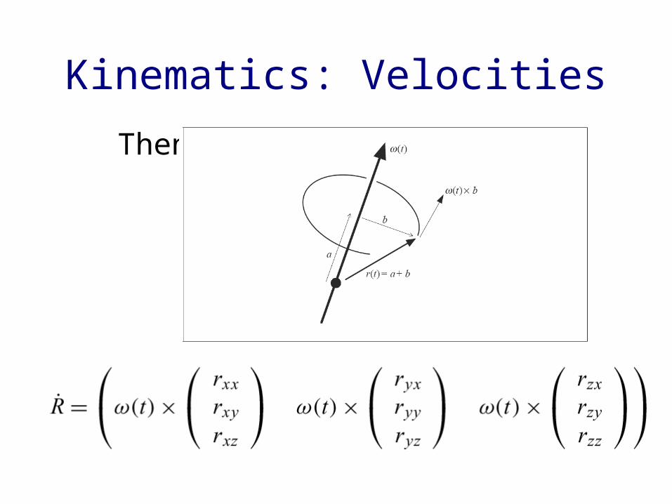
Kinematics: Velocities

Then

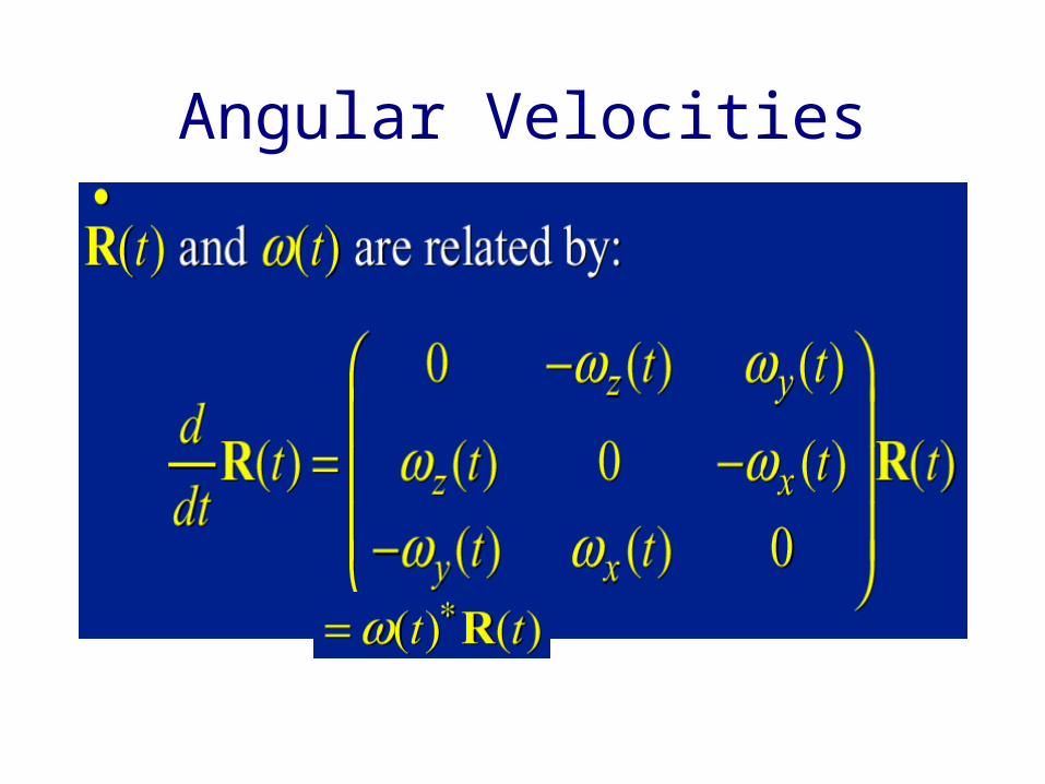
Angular Velocities

Dynamics: Accelerations

• How do v(t) and dR(t)/dt change over time?• First we need some more machinery

– Forces and Torques– Momentums– Inertia Tensor

• Simplify equations by formulating accelerations terms of momentum derivatives instead of velocity derivatives

Forces and Torques• External forces Fi(t) act on particles

– Total external force F= Fi(t)

• Torques depend on distance from the center of mass: i (t) = (ri(t) – x(t)) £ Fi(t)– Total external torque

= ((ri(t)-x(t)) £ Fi(t)

• F(t) doesn’t convey any information about where the various forces act

• (t) does tell us about the distribution of forces

Linear Momentum• Linear momentum P(t) lets us express the

effect of total force F(t) on body (simple, because of conservation of energy):

F(t) = dP(t)/dt• Linear momentum is the product of mass and

linear velocity– P(t) = midri(t)/dt

= miv(t) + (t) £ mi(ri(t)-x(t))• But, we work in body space:

– P(t)= miv(t)= Mv(t) (linear relationship)– Just as if body were a particle with mass M and

velocity v(t)– Derive v(t) to express acceleration:

dv(t)/dt = M-1 dP(t)/dt• Use P(t) instead of v(t) in state vectors

• Same thing, angular momentum L(t) allows us to express the effect of total torque (t) on the body:

• Similarily, there is a linear relationship between momentum and velocity:

– I(t) is inertia tensor, plays the role of

mass• Use L(t) instead of (t) in state vectors

Angular momentum

Inertia Tensor

• 3x3 matrix describing how the shape and mass distribution of the body affects the relationship between the angular velocity and the angular momentum I(t)

• Analogous to mass – rotational mass• We actually want the inverse I-1(t) for

computing (t)=I-1(t)L(t)

Inertia Tensor

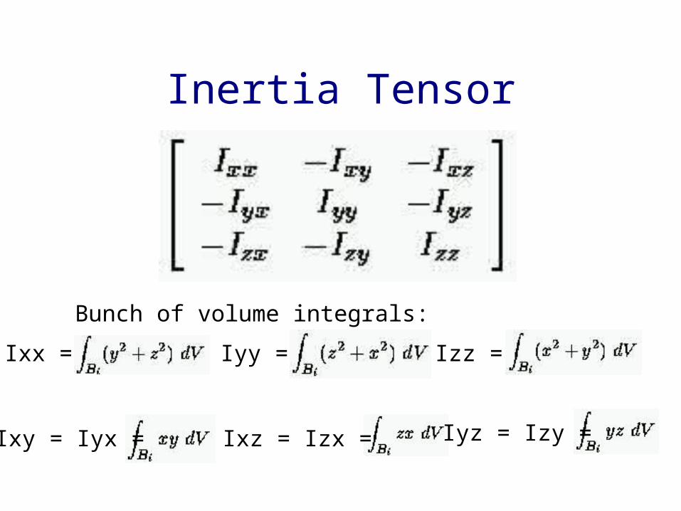
Ixx =

Ixy = Iyx =

Iyy = Izz =

Iyz = Izy =Ixz = Izx =

Bunch of volume integrals:

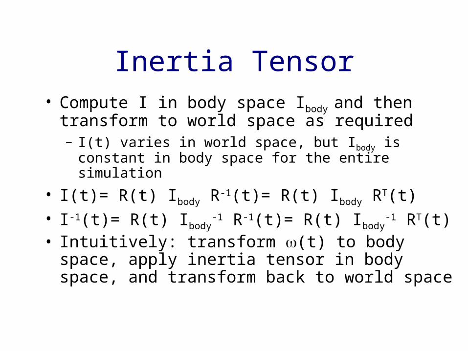
Inertia Tensor• Compute I in body space Ibody and then

transform to world space as required– I(t) varies in world space, but Ibody is constant in

body space for the entire simulation

• I(t)= R(t) Ibody R-1(t)= R(t) Ibody RT(t)• I-1(t)= R(t) Ibody

-1 R-1(t)= R(t) Ibody-1 RT(t)

• Intuitively: transform (t) to body space, apply inertia tensor in body space, and transform back to world space

Computing Ibody-1

• There exists an orientation in body space which causes Ixy, Ixz, Iyz to all vanish– Diagonalize tensor matrix, define the eigenvectors

to be the local body axes– Increases efficiency and trivial inverse

• Point sampling within the bounding box• Projection and evaluation of Greene’s thm.

– Code implementing this method exists– Refer to Mirtich’s paper at http://www.acm.org/jgt/papers/Mirtich96

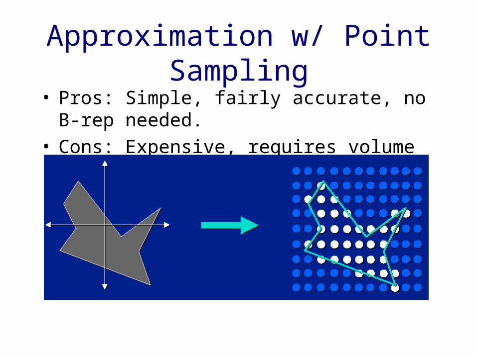
Approximation w/ Point Sampling

• Pros: Simple, fairly accurate, no B-rep needed.

• Cons: Expensive, requires volume test.

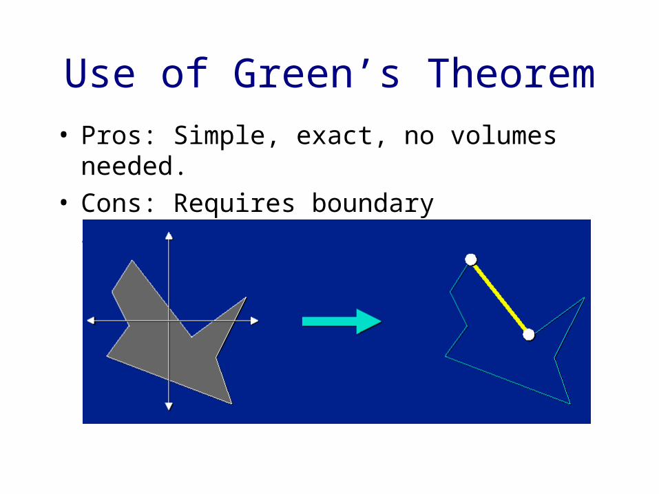
Use of Green’s Theorem• Pros: Simple, exact, no volumes

needed.• Cons: Requires boundary

representation.

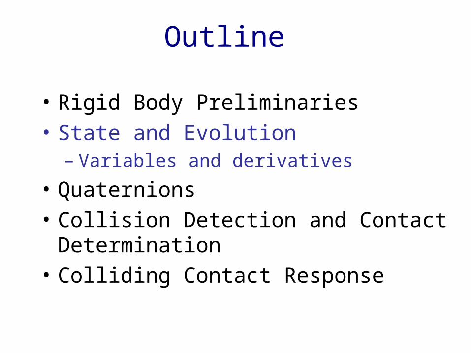
Outline

• Rigid Body Preliminaries• State and Evolution

– Variables and derivatives

• Quaternions• Collision Detection and Contact

Determination• Colliding Contact Response

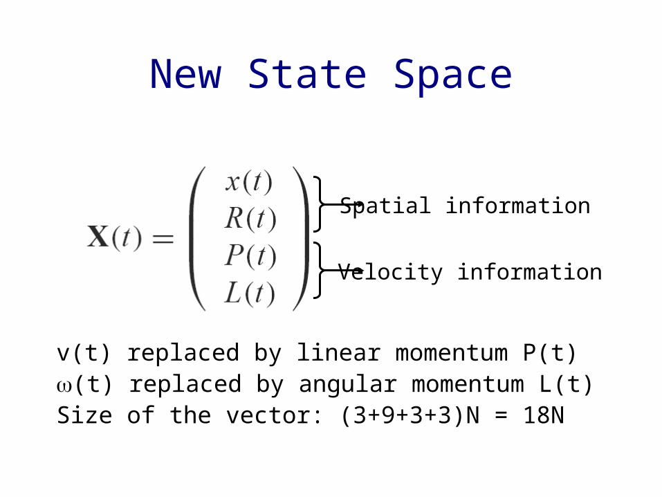
New State Space

v(t) replaced by linear momentum P(t)(t) replaced by angular momentum L(t)Size of the vector: (3+9+3+3)N = 18N

Spatial information

Velocity information

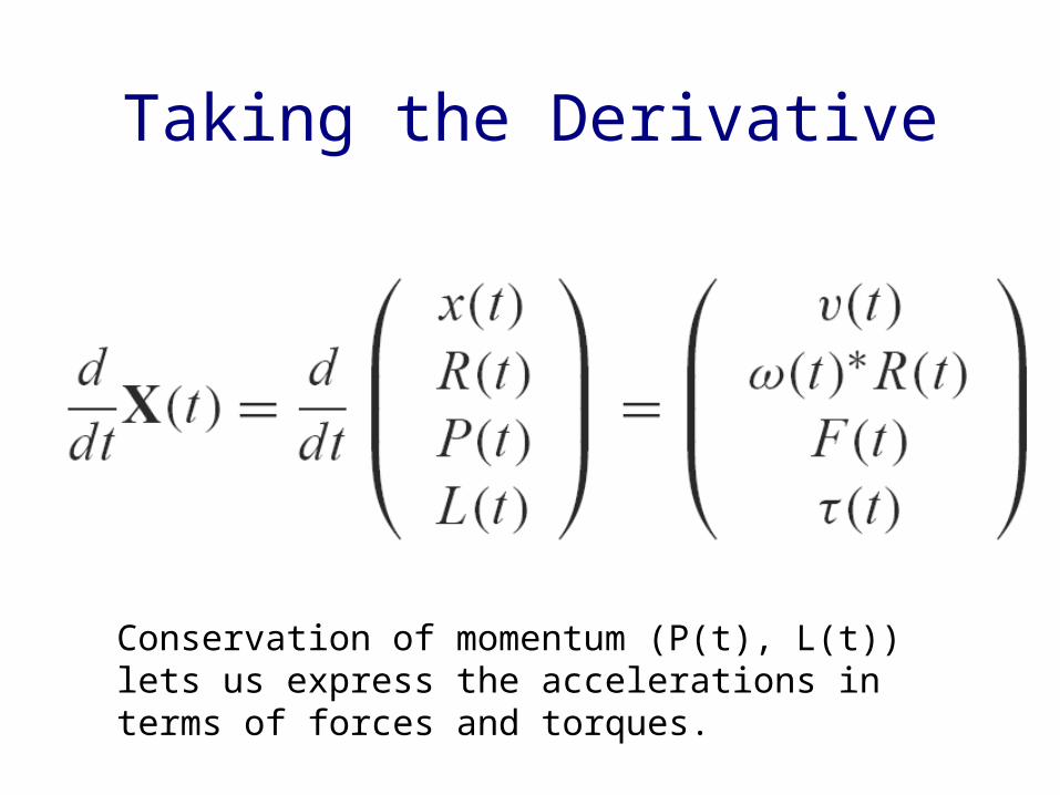
Taking the Derivative

Conservation of momentum (P(t), L(t)) lets us express the accelerations in terms of forces and torques.

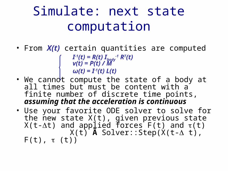
Simulate: next state computation

• From X(t) certain quantities are computedI-1(t) = R(t) Ibody

-1 RT(t) v(t) = P(t) / Mω(t) = I-1(t) L(t)

• We cannot compute the state of a body at all times but must be content with a finite number of discrete time points, assuming that the acceleration is continuous

• Use your favorite ODE solver to solve for the new state X(t), given previous state X(t-t) and applied forces F(t) and (t)

X(t) Ã Solver::Step(X(t- t), F(t), (t))

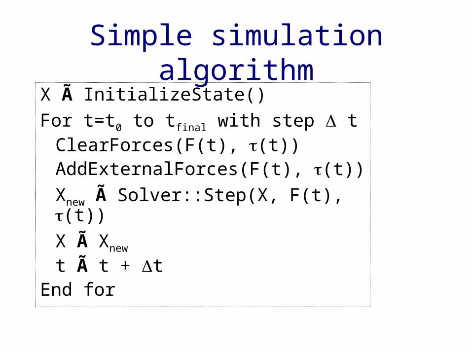
Simple simulation algorithm

X Ã InitializeState()For t=t0 to tfinal with step t

ClearForces(F(t), (t))AddExternalForces(F(t), (t))Xnew à Solver::Step(X, F(t), (t))X à Xnew

t à t + tEnd for

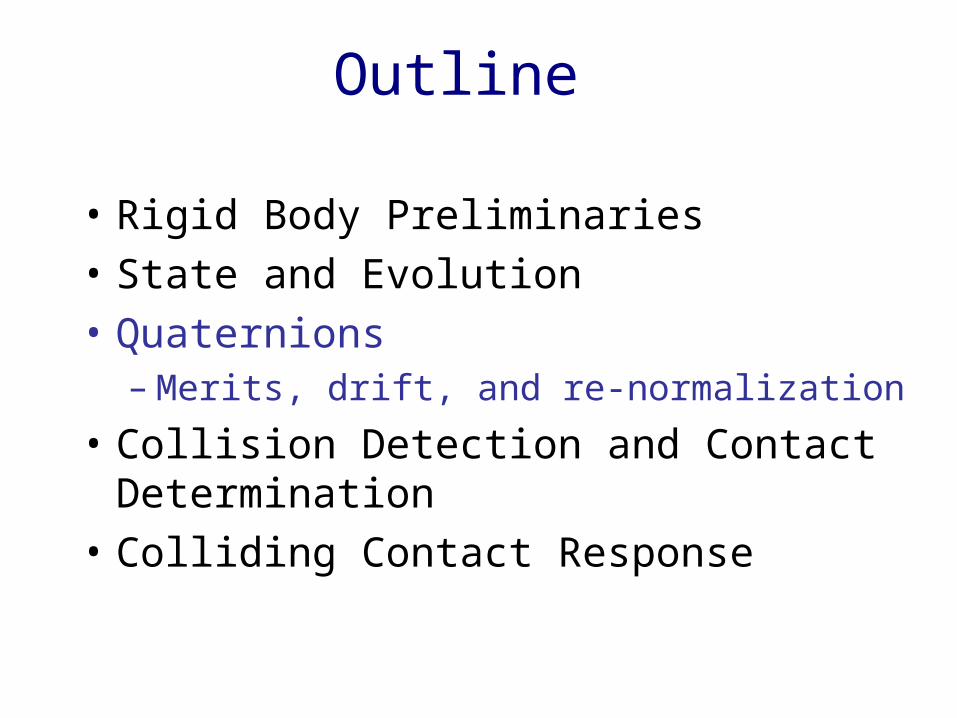
Outline

• Rigid Body Preliminaries• State and Evolution• Quaternions

– Merits, drift, and re-normalization

• Collision Detection and Contact Determination

• Colliding Contact Response

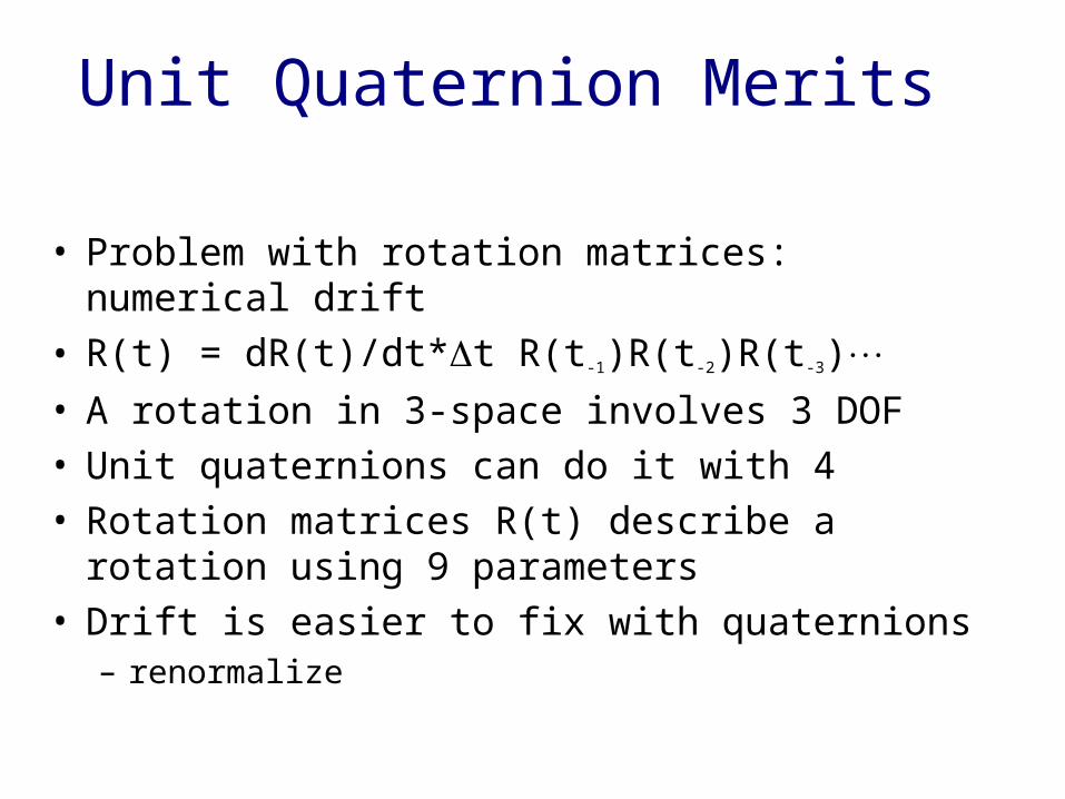
Unit Quaternion Merits

• Problem with rotation matrices: numerical drift

• R(t) = dR(t)/dt*t R(t-1)R(t-2)R(t-3)• A rotation in 3-space involves 3 DOF• Unit quaternions can do it with 4• Rotation matrices R(t) describe a rotation

using 9 parameters• Drift is easier to fix with quaternions

– renormalize

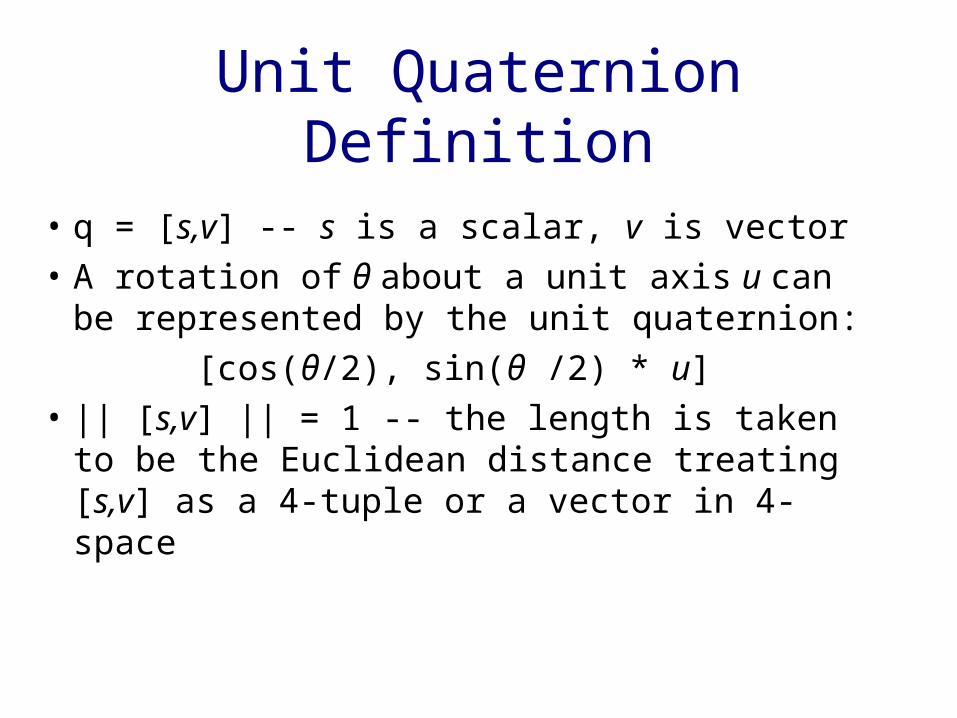
Unit Quaternion Definition

• q = [s,v] -- s is a scalar, v is vector• A rotation of θ about a unit axis u can

be represented by the unit quaternion:[cos(θ/2), sin(θ /2) * u]

• || [s,v] || = 1 -- the length is taken to be the Euclidean distance treating [s,v] as a 4-tuple or a vector in 4-space

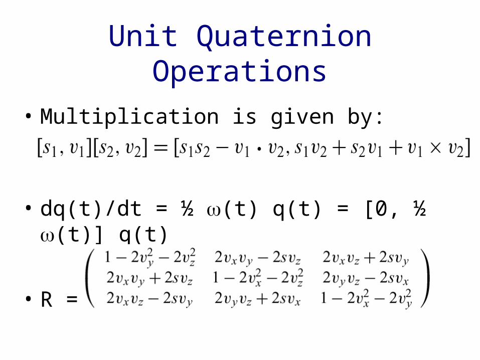
Unit Quaternion Operations

• Multiplication is given by:

• dq(t)/dt = ½ (t) q(t) = [0, ½ (t)] q(t)

• R =

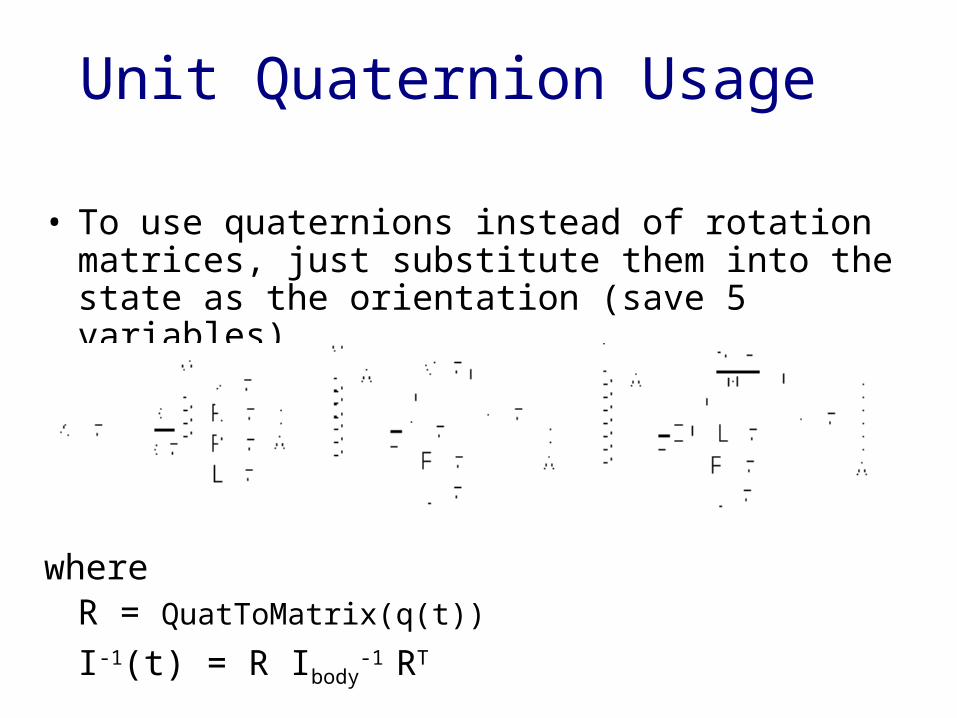
Unit Quaternion Usage

• To use quaternions instead of rotation matrices, just substitute them into the state as the orientation (save 5 variables)

where R = QuatToMatrix(q(t))

I-1(t) = R Ibody-1 RT

Outline

• Rigid Body Preliminaries• State and Evolution• Quaternions• Collision Detection and Contact

Determination– Contact classification– Intersection testing, bisection, and nearest

features

• Colliding Contact Response

What happens when bodies collide?

• Colliding– Bodies bounce off each other– Elasticity governs ‘bounciness’– Motion of bodies changes discontinuously

within a discrete time step– ‘Before’ and ‘After’ states need to be

computed

• In contact– Resting– Sliding– Friction

Detecting collisions and response

• Several choices– Collision detection: which algorithm?– Response: Backtrack or allow

penetration?

• Two primitives to find out if response is necessary:– Distance(A,B): cheap, no contact

information ! fast intersection query– Contact(A,B): expensive, with contact

information

Distance(A,B)

• Returns a value which is the minimum distance between two bodies

• Approximate may be ok• Negative if the bodies intersect• Convex polyhedra

– Lin-Canny and GJK -- 2 classes of algorithms

• Non-convex polyhedra– much more useful but hard to get distance fast– PQP/RAPID/SWIFT++

• Remark: most of these algorithms give inaccurate information if bodies intersect, except for DEEP

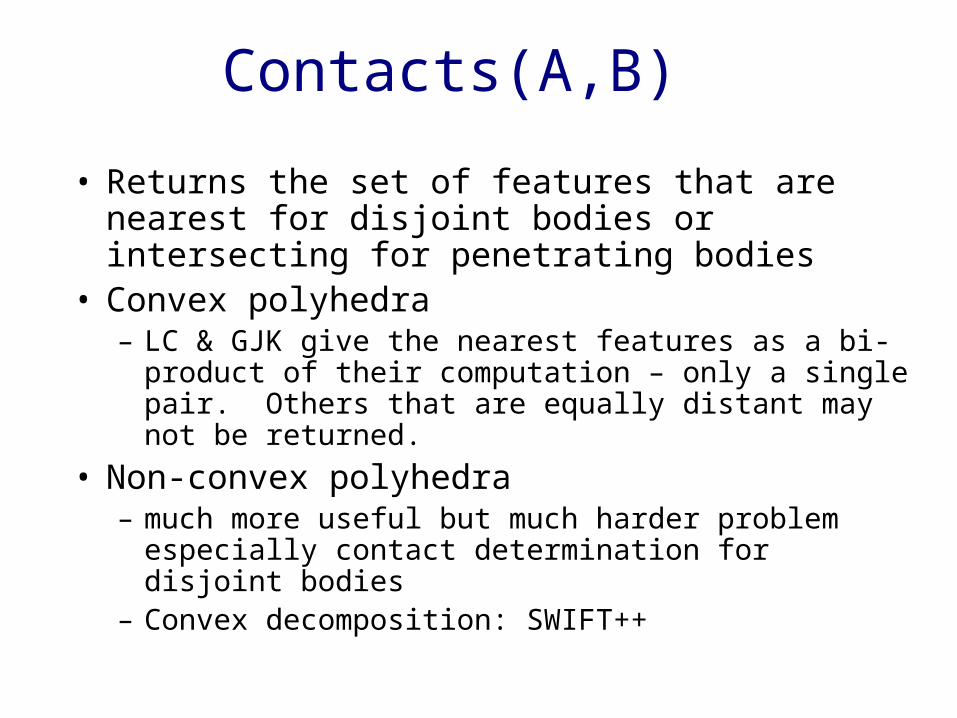
Contacts(A,B)

• Returns the set of features that are nearest for disjoint bodies or intersecting for penetrating bodies

• Convex polyhedra– LC & GJK give the nearest features as a bi-product

of their computation – only a single pair. Others that are equally distant may not be returned.

• Non-convex polyhedra– much more useful but much harder problem

especially contact determination for disjoint bodies

– Convex decomposition: SWIFT++

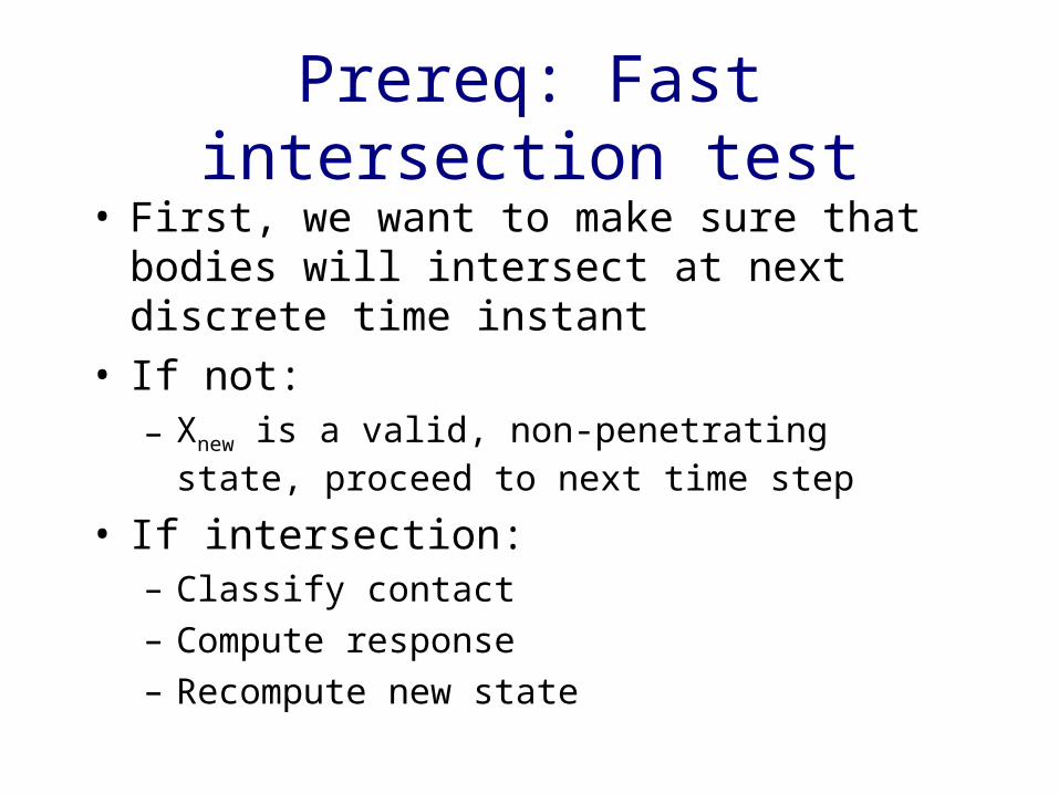
Prereq: Fast intersection test

• First, we want to make sure that bodies will intersect at next discrete time instant

• If not:– Xnew is a valid, non-penetrating state,

proceed to next time step

• If intersection:– Classify contact– Compute response– Recompute new state

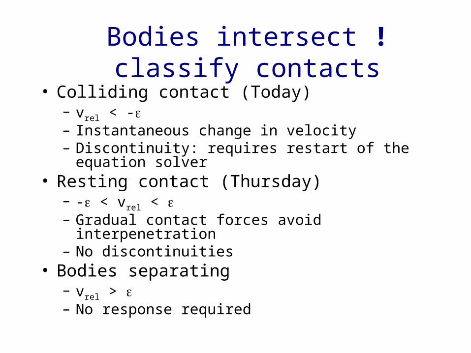
Bodies intersect ! classify contacts

• Colliding contact (Today)– vrel < -– Instantaneous change in velocity – Discontinuity: requires restart of the equation

solver• Resting contact (Thursday)

– - < vrel < – Gradual contact forces avoid interpenetration– No discontinuities

• Bodies separating– vrel > – No response required

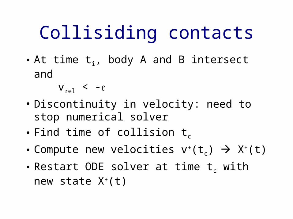
Collisiding contacts

• At time ti, body A and B intersect andvrel < -

• Discontinuity in velocity: need to stop numerical solver

• Find time of collision tc

• Compute new velocities v+(tc) X+(t)

• Restart ODE solver at time tc with new state X+(t)

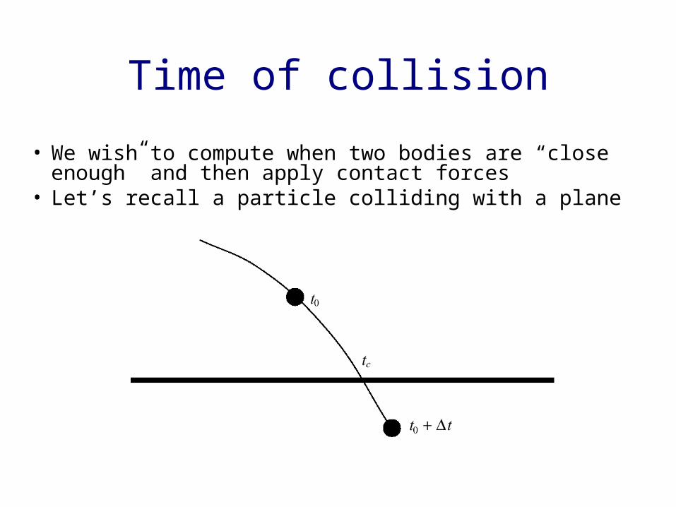
Time of collision

• We wish to compute when two bodies are “close enough” and then apply contact forces

• Let’s recall a particle colliding with a plane

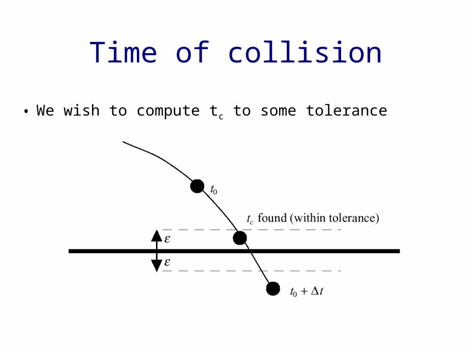
Time of collision

• We wish to compute tc to some tolerance

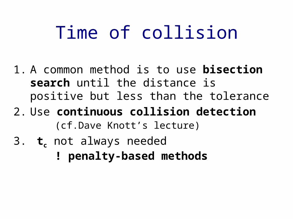
Time of collision

1. A common method is to use bisection search until the distance is positive but less than the tolerance

2. Use continuous collision detection (cf.Dave Knott’s

lecture)

3. tc not always needed ! penalty-based methods

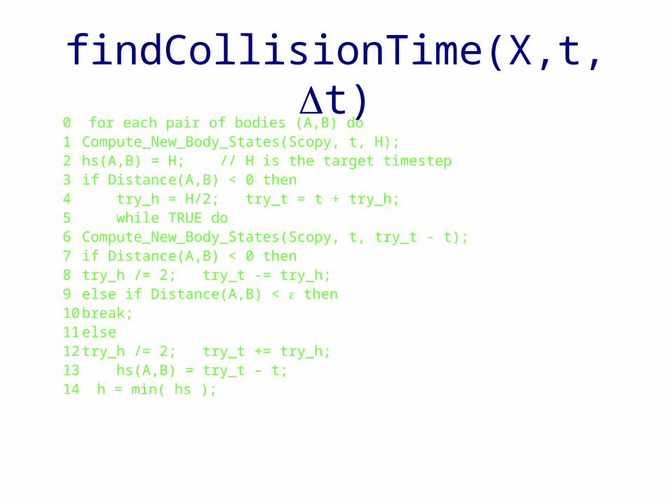
findCollisionTime(X,t,t)0 for each pair of bodies (A,B) do1 Compute_New_Body_States(Scopy, t, H);2 hs(A,B) = H; // H is the target timestep3 if Distance(A,B) < 0 then4 try_h = H/2; try_t = t + try_h;5 while TRUE do6 Compute_New_Body_States(Scopy, t, try_t - t);7 if Distance(A,B) < 0 then8 try_h /= 2; try_t -= try_h;9 else if Distance(A,B) < then10 break;11 else12 try_h /= 2; try_t += try_h;13 hs(A,B) = try_t – t;14 h = min( hs );

Outline

• Rigid Body Preliminaries• State and Evolution• Quaternions• Collision Detection and Contact

Determination• Colliding Contact Response

– Normal vector, restitution, and force application

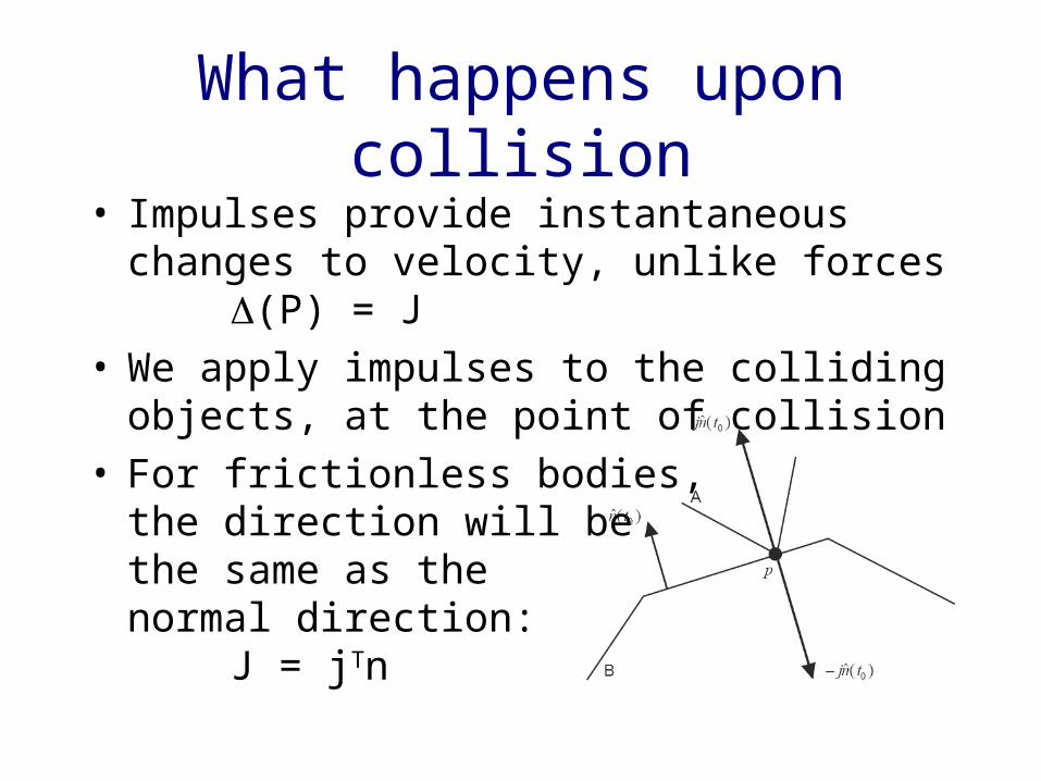
What happens upon collision

• Impulses provide instantaneous changes to velocity, unlike forces

(P) = J• We apply impulses to the colliding

objects, at the point of collision• For frictionless bodies,

the direction will be the same as the normal direction:

J = jTn

Colliding Contact Response

• Assumptions:– Convex bodies– Non-penetrating– Non-degenerate configuration

• edge-edge or vertex-face• appropriate set of rules can handle the others

• Need a contact unit normal vector– Face-vertex case: use the normal of the face– Edge-edge case: use the cross-product of the

direction vectors of the two edges

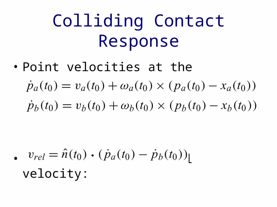
Colliding Contact Response

• Point velocities at the nearest points:

• Relative contact normal velocity:

Colliding Contact Response

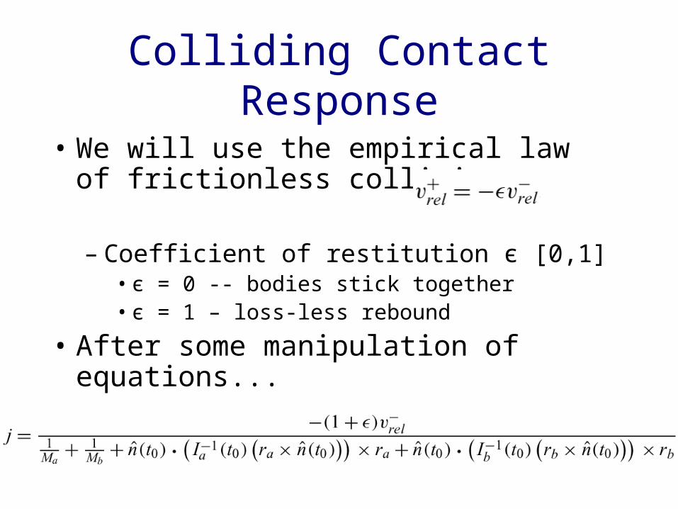
• We will use the empirical law of frictionless collisions:

– Coefficient of restitution є [0,1]• є = 0 -- bodies stick together• є = 1 – loss-less rebound

• After some manipulation of equations...

Apply_BB_Forces()

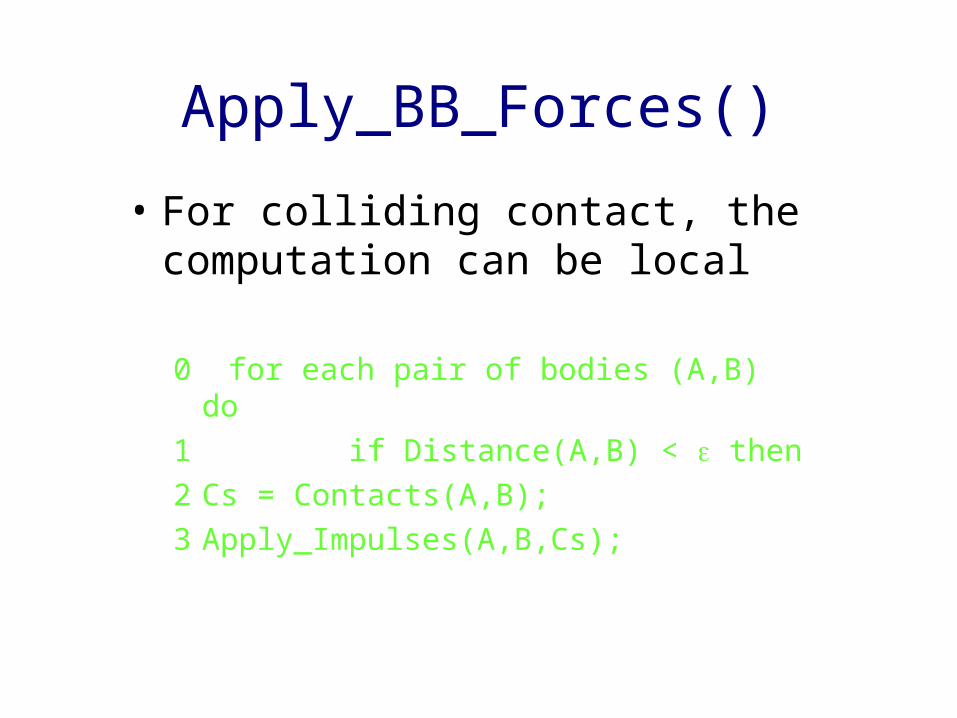
• For colliding contact, the computation can be local

0 for each pair of bodies (A,B) do1 if Distance(A,B) < then2 Cs = Contacts(A,B);3 Apply_Impulses(A,B,Cs);

Apply_Impulses(A,B,Cs)

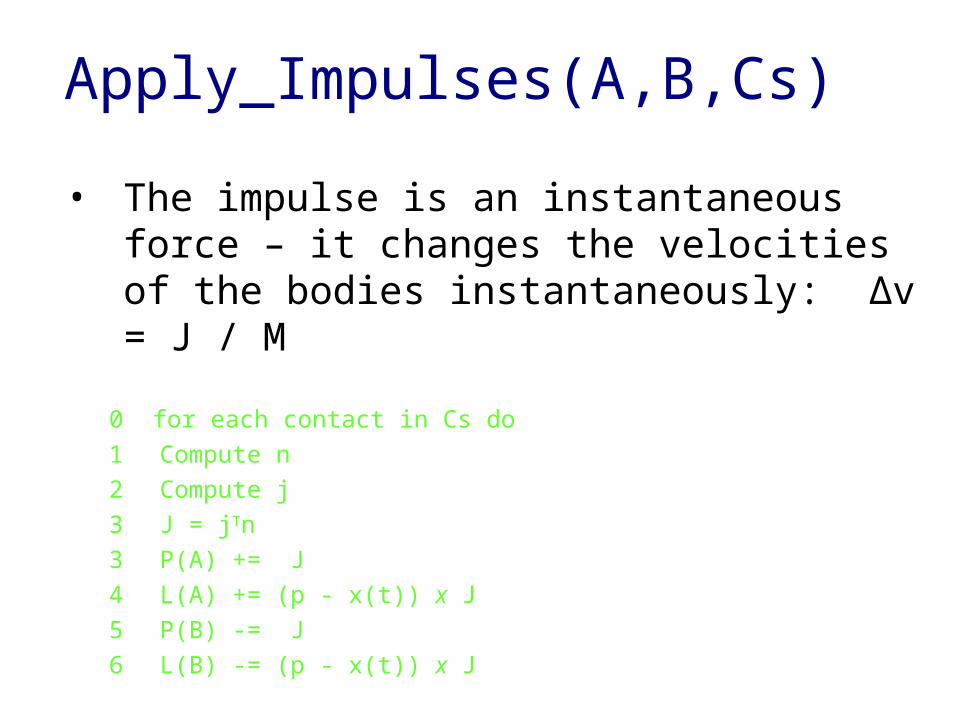
• The impulse is an instantaneous force – it changes the velocities of the bodies instantaneously: Δv = J / M

0 for each contact in Cs do1 Compute n2 Compute j3 J = jTn3 P(A) += J4 L(A) += (p - x(t)) x J5 P(B) -= J6 L(B) -= (p - x(t)) x J

Simulation algorithm with Collisions

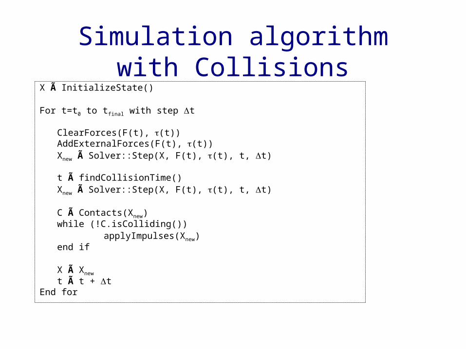
X Ã InitializeState()

For t=t0 to tfinal with step t

ClearForces(F(t), (t))AddExternalForces(F(t), (t))Xnew à Solver::Step(X, F(t), (t), t, t)

t à findCollisionTime()Xnew à Solver::Step(X, F(t), (t), t, t)

C Ã Contacts(Xnew)while (!C.isColliding())

applyImpulses(Xnew)end if

X Ã Xnew

t à t + tEnd for

Penalty Methods

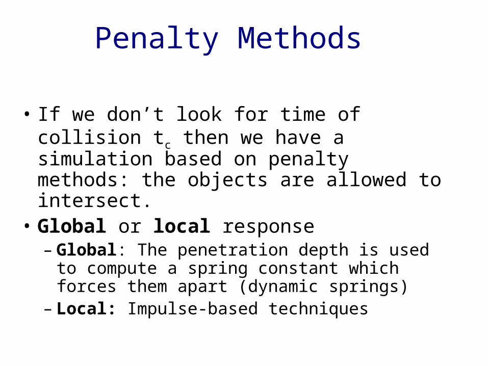
• If we don’t look for time of collision tc then we have a simulation based on penalty methods: the objects are allowed to intersect.

• Global or local response– Global: The penetration depth is used

to compute a spring constant which forces them apart (dynamic springs)

– Local: Impulse-based techniques

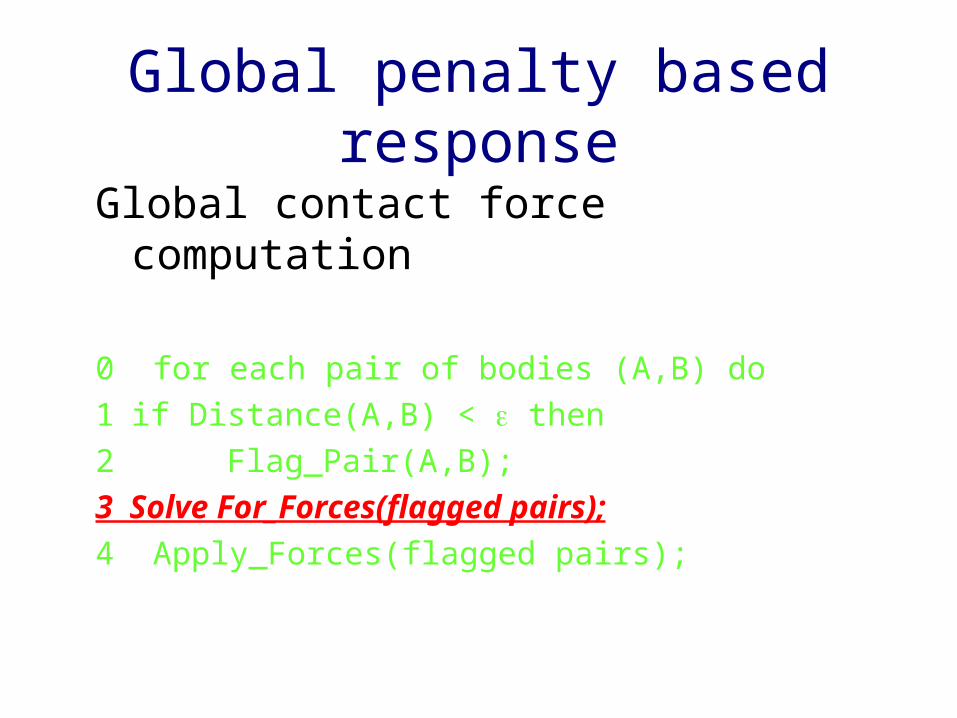
Global penalty based response

Global contact force computation

0 for each pair of bodies (A,B) do1 if Distance(A,B) < then2 Flag_Pair(A,B);3 Solve For_Forces(flagged pairs);4 Apply_Forces(flagged pairs);

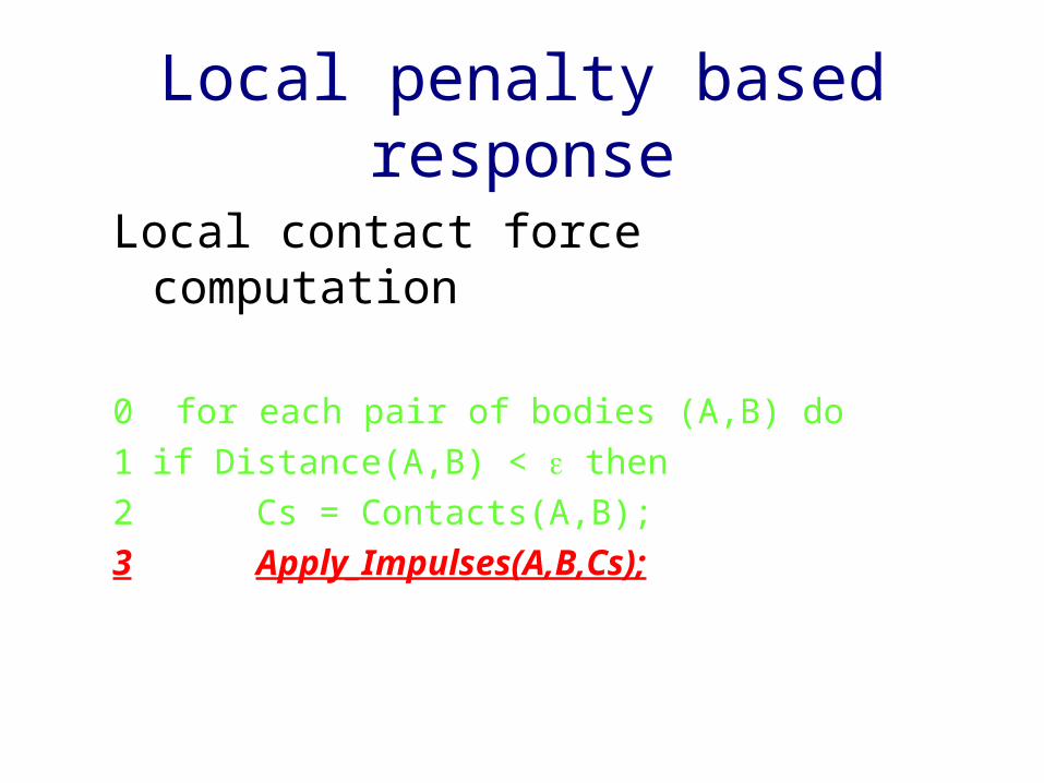
Local penalty based response

Local contact force computation

0 for each pair of bodies (A,B) do1 if Distance(A,B) < then2 Cs = Contacts(A,B); 3 Apply_Impulses(A,B,Cs);

References

• D. Baraff and A. Witkin, “Physically Based Modeling: Principles and Practice,” Course Notes, SIGGRAPH 2001.

• B. Mirtich, “Fast and Accurate Computation of Polyhedral Mass Properties,” Journal of Graphics Tools, volume 1, number 2, 1996.

• D. Baraff, “Dynamic Simulation of Non-Penetrating Rigid Bodies”, Ph.D. thesis, Cornell University, 1992.

• B. Mirtich and J. Canny, “Impulse-based Simulation of Rigid Bodies,” in Proceedings of 1995 Symposium on Interactive 3D Graphics, April 1995.

• B. Mirtich, “Impulse-based Dynamic Simulation of Rigid Body Systems,” Ph.D. thesis, University of California, Berkeley, December, 1996.

• B. Mirtich, “Hybrid Simulation: Combining Constraints and Impulses,” in Proceedings of First Workshop on Simulation and Interaction in Virtual Environments, July 1995.

• COMP259 Rigid Body Simulation Slides, Chris Vanderknyff 2004