Rigid Body Dynamics 2

CSE169: Computer Animation

Instructor: Steve Rotenberg

UCSD, Winter 2017

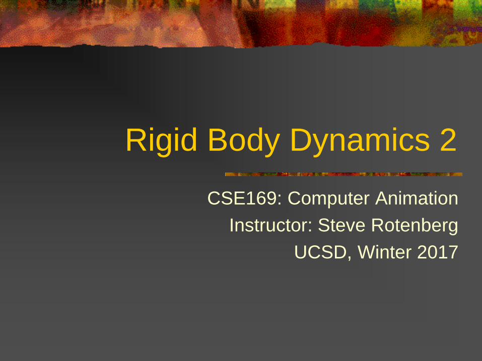
Cross Product & Hat Operator

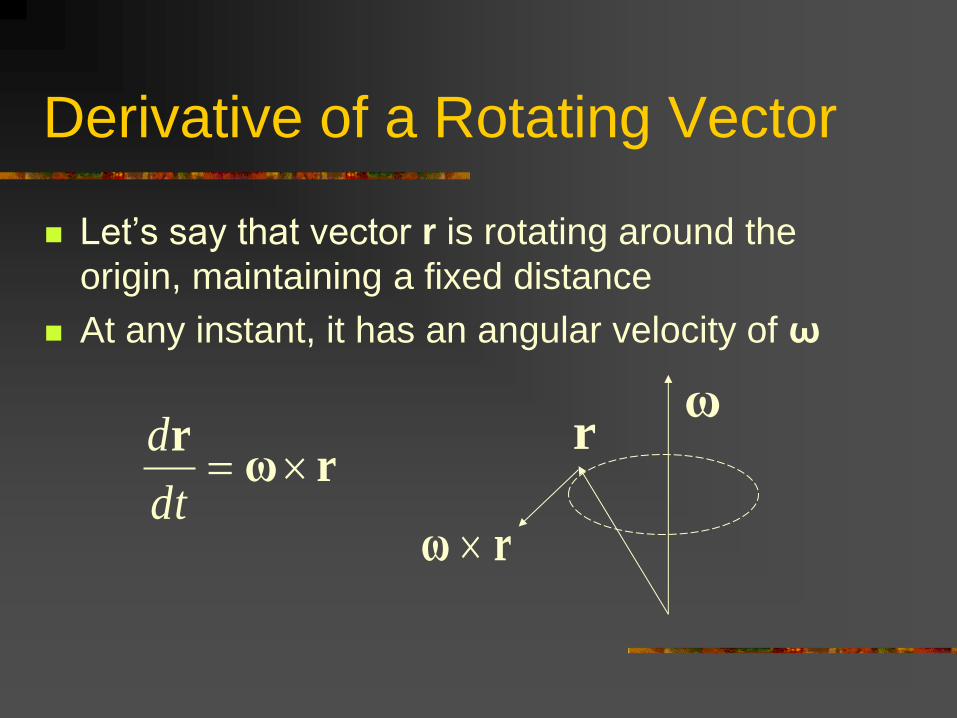
Derivative of a Rotating Vector

Let’s say that vector r is rotating around the

origin, maintaining a fixed distance

At any instant, it has an angular velocity of ω

rωr

dt

d

rω

rω

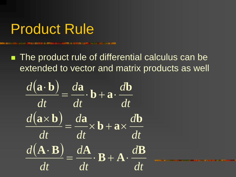
Product Rule

The product rule of differential calculus can be

extended to vector and matrix products as well

dt

d

dt

d

dt

d

dt

d

dt

d

dt

d

dt

d

dt

d

dt

d

BAB

ABA

bab

aba

bab

aba

Rigid Bodies

We treat a rigid body as a system of particles, where the distance between any two particles is fixed

We will assume that internal forces are generated to hold the relative positions fixed. These internal forces are all balanced out with Newton’s third law, so that they all cancel out and have no effect on the total momentum or angular momentum

The rigid body can actually have an infinite number of particles, spread out over a finite volume

Instead of mass being concentrated at discrete points, we will consider the density as being variable over the volume

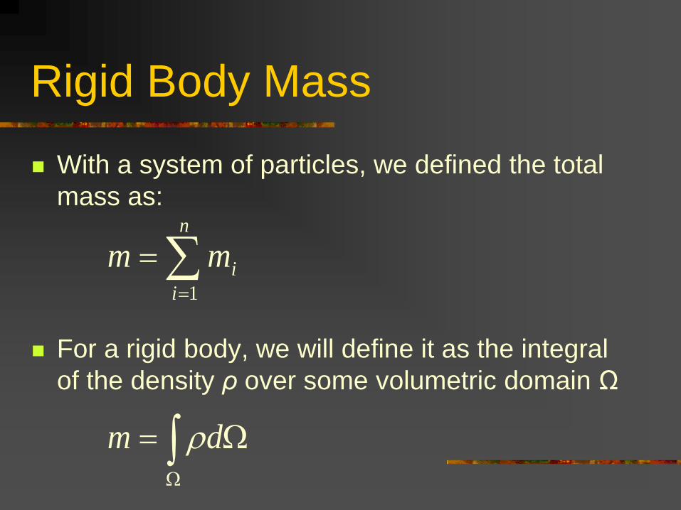
Rigid Body Mass

With a system of particles, we defined the total

mass as:

For a rigid body, we will define it as the integral

of the density ρ over some volumetric domain Ω

dm

n

i

imm1

Angular Momentum

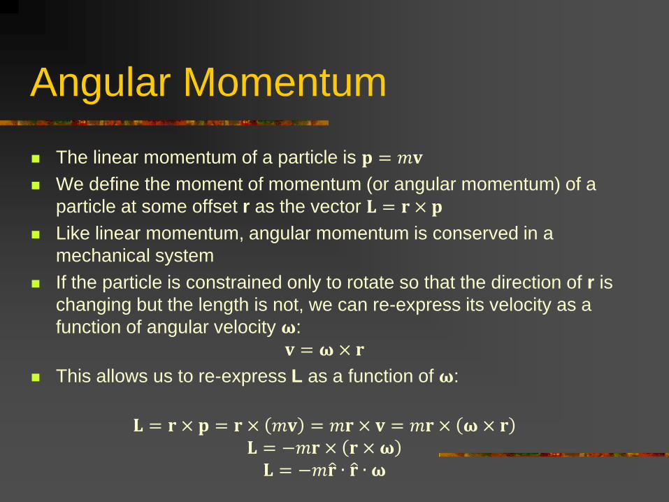
The linear momentum of a particle is 𝐩 = 𝑚𝐯

We define the moment of momentum (or angular momentum) of a

particle at some offset r as the vector 𝐋 = 𝐫 × 𝐩

Like linear momentum, angular momentum is conserved in a

mechanical system

If the particle is constrained only to rotate so that the direction of r is

changing but the length is not, we can re-express its velocity as a

function of angular velocity 𝛚:

𝐯 = 𝛚 × 𝐫

This allows us to re-express L as a function of 𝛚:

𝐋 = 𝐫 × 𝐩 = 𝐫 × 𝑚𝐯 = 𝑚𝐫 × 𝐯 = 𝑚𝐫 × 𝛚 × 𝐫

𝐋 = −𝑚𝐫 × 𝐫 × 𝛚

𝐋 = −𝑚𝐫 ∙ 𝐫 ∙ 𝛚

Rotational Inertia

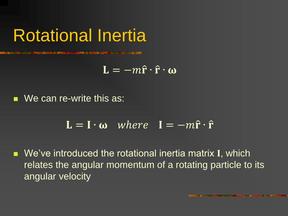
𝐋 = −𝑚𝐫 ∙ 𝐫 ∙ 𝛚

We can re-write this as:

𝐋 = 𝐈 ∙ 𝛚 𝑤ℎ𝑒𝑟𝑒 𝐈 = −𝑚𝐫 ∙ 𝐫

We’ve introduced the rotational inertia matrix 𝐈, which

relates the angular momentum of a rotating particle to its

angular velocity

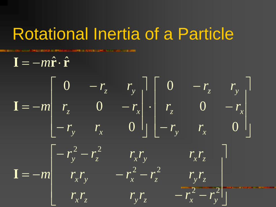
Rotational Inertia of a Particle

22

22

22

0

0

0

0

0

0

ˆˆ

yxzyzx

zyzxyx

zxyxzy

xy

xz

yz

xy

xz

yz

rrrrrr

rrrrrr

rrrrrr

m

rr

rr

rr

rr

rr

rr

m

m

I

I

rrI

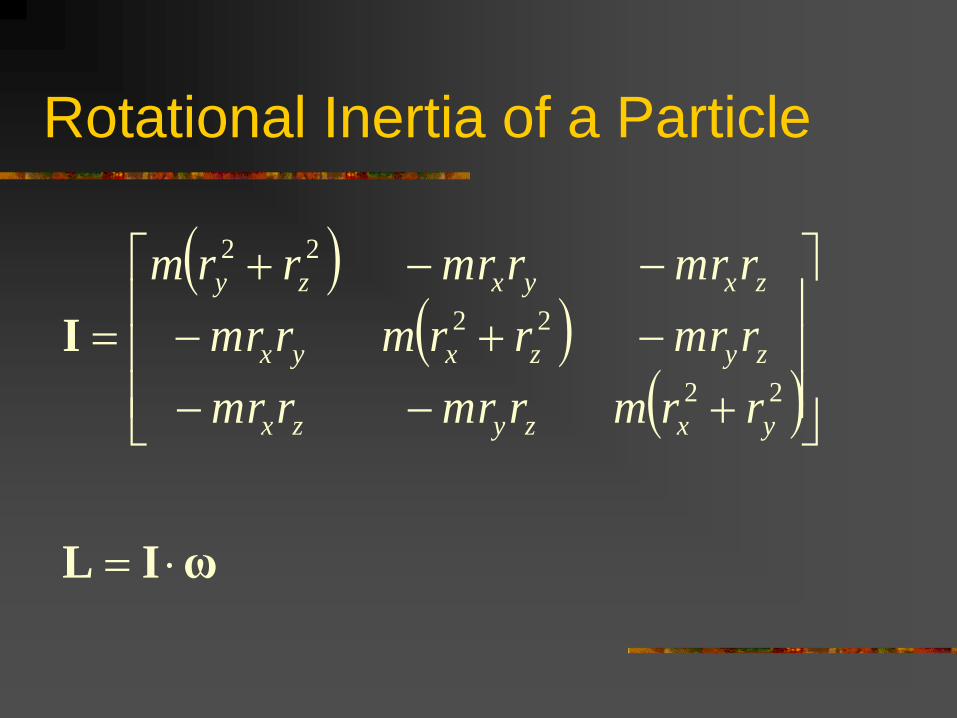
Rotational Inertia of a Particle

ωIL

I

22

22

22

yxzyzx

zyzxyx

zxyxzy

rrmrmrrmr

rmrrrmrmr

rmrrmrrrm

Rotational Inertia of a Rigid Body

For a rigid body, we replace the single

mass and position of the particle with an

integration over all of the points of the rigid

body times the density at that point

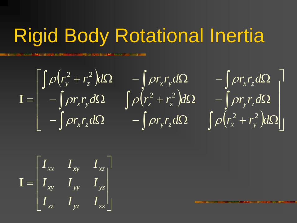
Rigid Body Rotational Inertia

zzyzxz

yzyyxy

xzxyxx

yxzyzx

zyzxyx

zxyxzy

III

III

III

drrdrrdrr

drrdrrdrr

drrdrrdrr

I

I

22

22

22

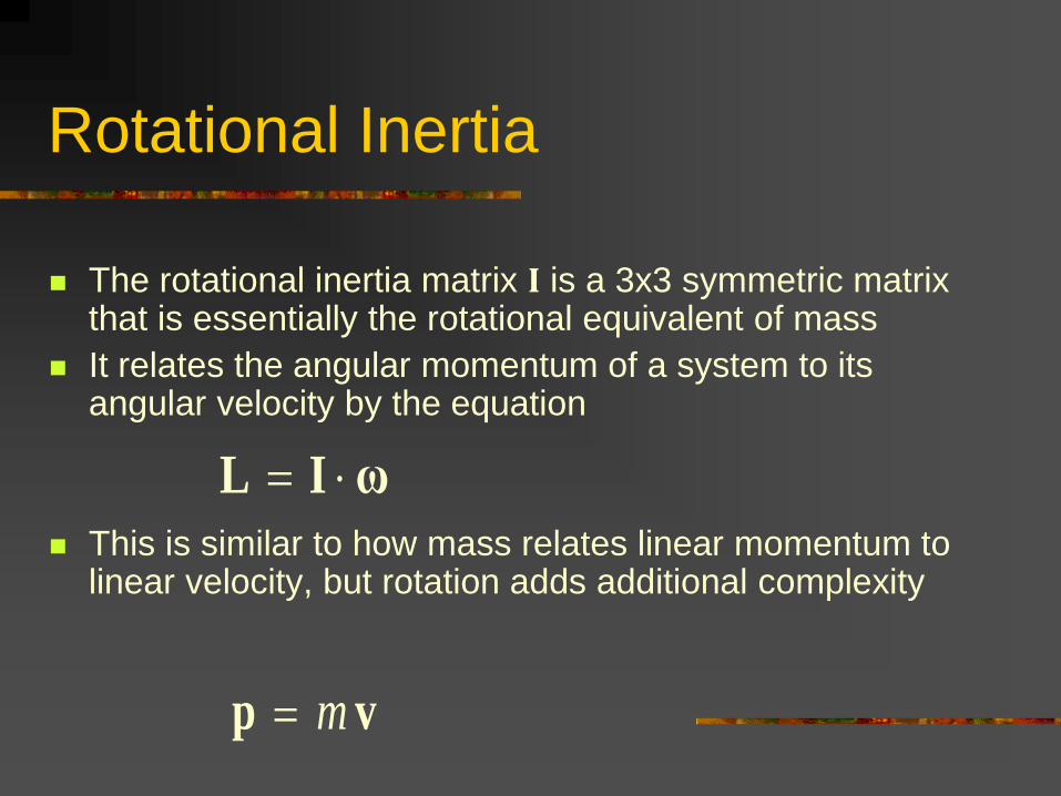
Rotational Inertia

The rotational inertia matrix 𝐈 is a 3x3 symmetric matrix that is essentially the rotational equivalent of mass

It relates the angular momentum of a system to its angular velocity by the equation

This is similar to how mass relates linear momentum to linear velocity, but rotation adds additional complexity

ωIL

vp m

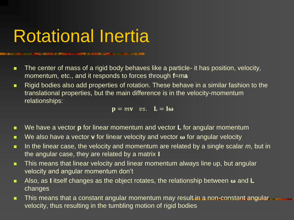
Rotational Inertia

The center of mass of a rigid body behaves like a particle- it has position, velocity,

momentum, etc., and it responds to forces through f=ma

Rigid bodies also add properties of rotation. These behave in a similar fashion to the

translational properties, but the main difference is in the velocity-momentum

relationships:

𝐩 = 𝑚𝐯 𝑣𝑠. 𝐋 = 𝐈𝛚

We have a vector p for linear momentum and vector L for angular momentum

We also have a vector v for linear velocity and vector 𝛚 for angular velocity

In the linear case, the velocity and momentum are related by a single scalar m, but in

the angular case, they are related by a matrix 𝐈

This means that linear velocity and linear momentum always line up, but angular

velocity and angular momentum don’t

Also, as 𝐈 itself changes as the object rotates, the relationship between 𝛚 and L

changes

This means that a constant angular momentum may result in a non-constant angular

velocity, thus resulting in the tumbling motion of rigid bodies

Rotational Inertia

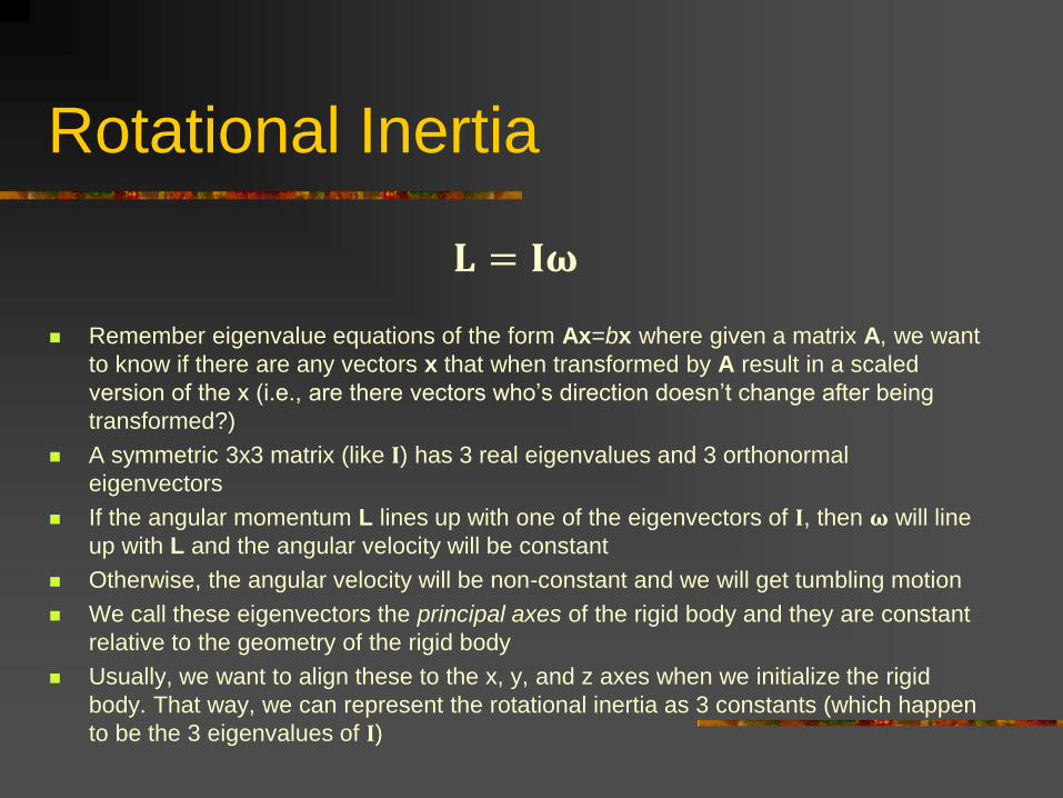
𝐋 = 𝐈𝛚

Remember eigenvalue equations of the form Ax=bx where given a matrix A, we want

to know if there are any vectors x that when transformed by A result in a scaled

version of the x (i.e., are there vectors who’s direction doesn’t change after being

transformed?)

A symmetric 3x3 matrix (like 𝐈) has 3 real eigenvalues and 3 orthonormal

eigenvectors

If the angular momentum L lines up with one of the eigenvectors of 𝐈, then 𝛚 will line

up with L and the angular velocity will be constant

Otherwise, the angular velocity will be non-constant and we will get tumbling motion

We call these eigenvectors the principal axes of the rigid body and they are constant

relative to the geometry of the rigid body

Usually, we want to align these to the x, y, and z axes when we initialize the rigid

body. That way, we can represent the rotational inertia as 3 constants (which happen

to be the 3 eigenvalues of 𝐈)

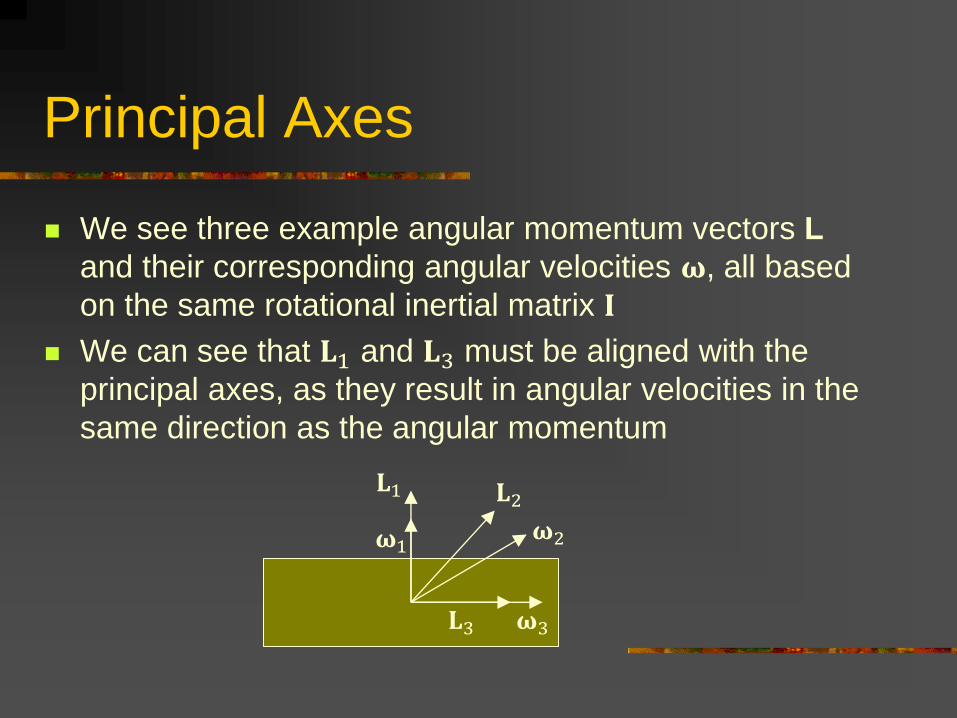
We see three example angular momentum vectors L

and their corresponding angular velocities 𝛚, all based

on the same rotational inertial matrix 𝐈

We can see that 𝐋1 and 𝐋3 must be aligned with the

principal axes, as they result in angular velocities in the

same direction as the angular momentum

Principal Axes

𝛚1

𝐋1

𝐋3 𝛚3

𝐋2

𝛚2

Principal Axes & Inertias

If we diagonalize the I matrix, we get an orientation

matrix A and a constant diagonal matrix Io

The matrix A rotates the object from an orientation

where the principal axes line up with the x, y, and z axes

The three values in Io, (namely Ix, Iy, and Iz) are the

principal inertias. They represent the resistance to

torque around the corresponding principal axis (in a

similar way that mass represents the resistance to force)

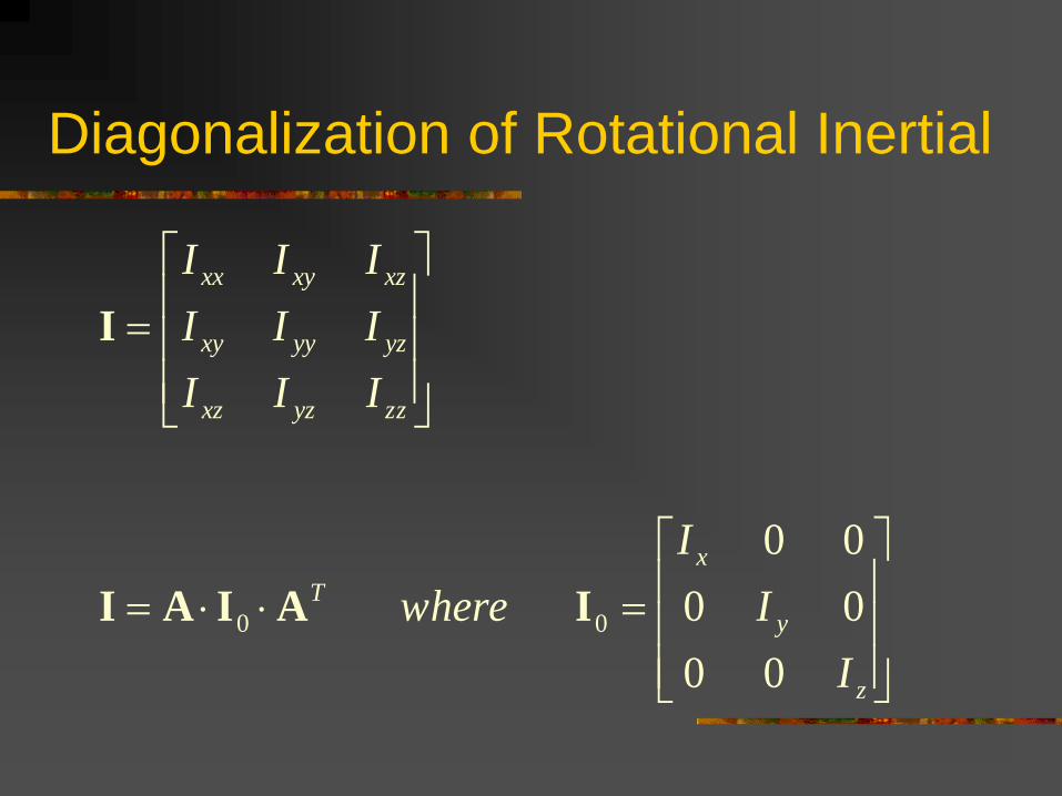
Diagonalization of Rotational Inertial

z

y

x

T

zzyzxz

yzyyxy

xzxyxx

I

I

I

where

III

III

III

00

00

00

00 IAIAI

I

Particle Dynamics

Position

Velocity

Acceleration

Mass

Momentum

Force

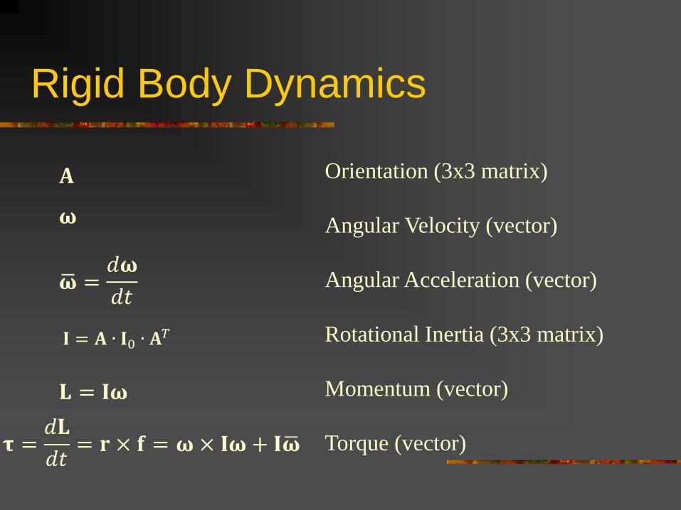
Rigid Body Dynamics

Orientation (3x3 matrix)

Angular Velocity (vector)

Angular Acceleration (vector)

Rotational Inertia (3x3 matrix)

Momentum (vector)

Torque (vector)

𝐈 = 𝐀 ∙ 𝐈0 ∙ 𝐀𝑇

Newton-Euler Equations

ωIωIωτ

af

m

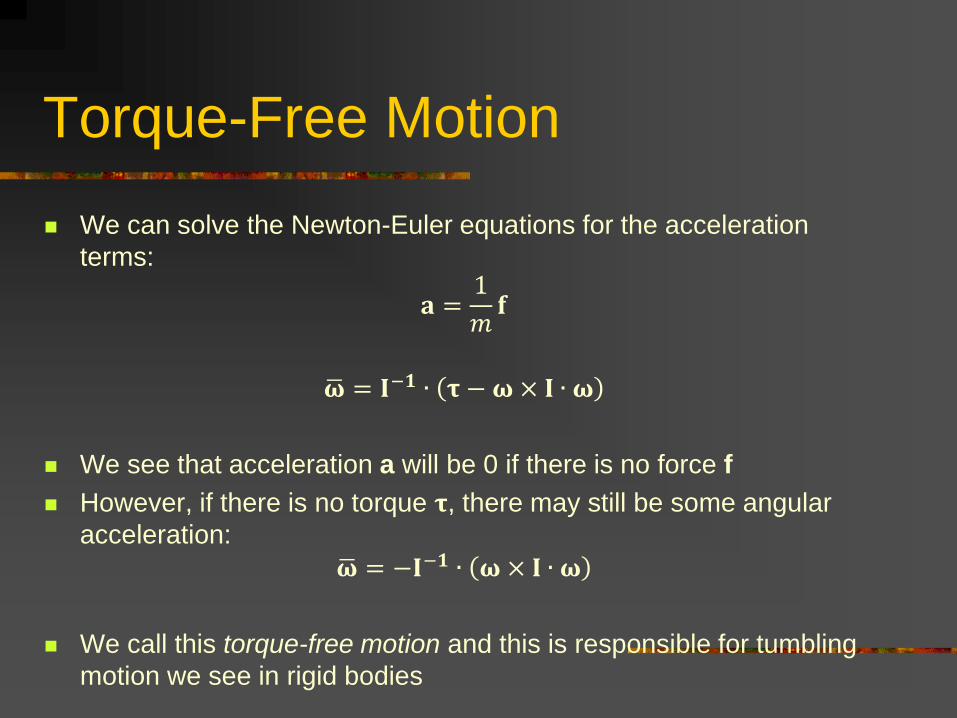
Torque-Free Motion

We can solve the Newton-Euler equations for the acceleration

terms:

𝐚 =1

𝑚𝐟

𝛚 = 𝐈−𝟏 ∙ 𝛕 − 𝛚 × 𝐈 ∙ 𝛚

We see that acceleration a will be 0 if there is no force f

However, if there is no torque 𝛕, there may still be some angular

acceleration:

𝛚 = −𝐈−𝟏 ∙ 𝛚 × 𝐈 ∙ 𝛚

We call this torque-free motion and this is responsible for tumbling

motion we see in rigid bodies

Rigid Body Simulation

Each frame, we can apply several forces to the rigid body, that sum up to one total

force and one total torque

𝐟 = 𝐟𝑖 𝛕 = 𝐫𝑖 × 𝐟𝑖

We can then integrate the force and torque over the time step to get the new linear

and angular momenta

𝐩′ = 𝐩 + 𝐟∆𝑡 𝐋′ = 𝐋 + 𝛕∆𝑡

We can then compute the linear and angular velocities from those:

𝐯 =1

𝑚𝐩′ 𝛚 = 𝐈−1𝐋′

We can now integrate the new position and orientation:

𝐱′ = 𝐱 + 𝐯∆𝑡 𝐀′ = 𝐀 ∙ 𝑅𝑜𝑡𝑎𝑡𝑒(𝛚∆𝑡)

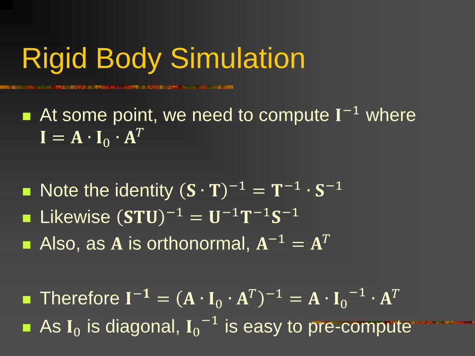
Rigid Body Simulation

At some point, we need to compute 𝐈−1 where

𝐈 = 𝐀 ∙ 𝐈0 ∙ 𝐀𝑇

Note the identity 𝐒 ∙ 𝐓 −1 = 𝐓−1 ∙ 𝐒−1

Likewise 𝐒𝐓𝐔 −1 = 𝐔−1𝐓−1𝐒−1

Also, as 𝐀 is orthonormal, 𝐀−1 = 𝐀𝑇

Therefore 𝐈−𝟏 = 𝐀 ∙ 𝐈0 ∙ 𝐀𝑇 −1 = 𝐀 ∙ 𝐈0−1 ∙ 𝐀𝑇

As 𝐈0 is diagonal, 𝐈0−1 is easy to pre-compute

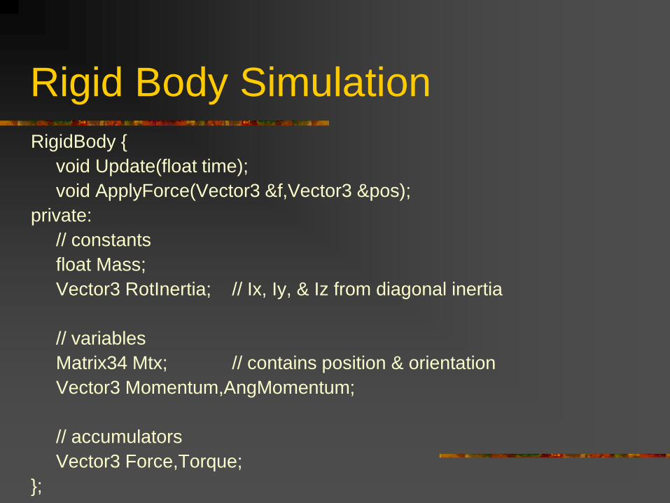
Rigid Body Simulation

RigidBody {

void Update(float time);

void ApplyForce(Vector3 &f,Vector3 &pos);

private:

// constants

float Mass;

Vector3 RotInertia; // Ix, Iy, & Iz from diagonal inertia

// variables

Matrix34 Mtx; // contains position & orientation

Vector3 Momentum,AngMomentum;

// accumulators

Vector3 Force,Torque;

};

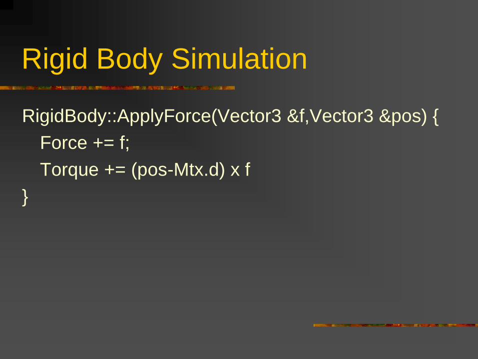
Rigid Body Simulation

RigidBody::ApplyForce(Vector3 &f,Vector3 &pos) {

Force += f;

Torque += (pos-Mtx.d) x f

}

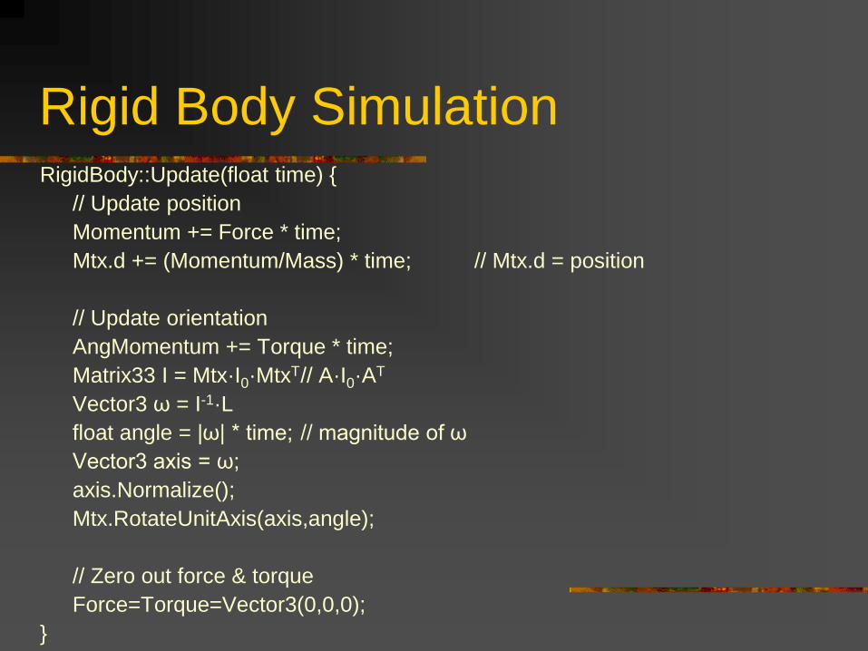
Rigid Body Simulation RigidBody::Update(float time) {

// Update position

Momentum += Force * time;

Mtx.d += (Momentum/Mass) * time; // Mtx.d = position

// Update orientation

AngMomentum += Torque * time;

Matrix33 I = Mtx·I0·MtxT // A·I0·AT

Vector3 ω = I-1·L

float angle = |ω| * time; // magnitude of ω

Vector3 axis = ω;

axis.Normalize();

Mtx.RotateUnitAxis(axis,angle);

// Zero out force & torque

Force=Torque=Vector3(0,0,0);

}

Rigid Body Set-Up

To define a rigid body from a physics point of view, we need only 4

constants: its mass m, and its principal rotational inertias 𝐼𝑥, 𝐼𝑦, and

𝐼𝑧

For collision detection and rendering, we will also want some type of

geometry- and we can calculate the inertia properties from this

We expect that the geometry for the rigid body is positioned such

that the center of mass lies at the origin and that the principal axes

line up with x, y, and z

One way to do this is to use simple shapes like spheres and boxes.

We can use simple formulas to calculate m, 𝐼𝑥, 𝐼𝑦, and 𝐼𝑧 from the

dimensions and density (see last lecture for some of these)

Alternately, we can use a triangle mesh as input and calculate the

inertia properties from that

Mirtich-Eberly Algorithm

In 1996, Brian Mirtich published an algorithm for analytically

calculating the inertia properties of a polygonal mesh and in 2002,

David Eberly streamlined the algorithm specifically for triangle

meshes

The resulting algorithm loops through each triangle, makes several

relatively simple calculations per triangle, and ultimately ends up

with exact values for the total volume, center of mass, and all 6

rotational inertia integrals

We could conceivably input any mesh, calculate the properties, and

then re-center the mesh to move the center of mass to the origin,

and then diagonalize the rotational inertia matrix and re-rotate the

mesh by the resulting rotation to align the principal axes with x, y,

and z

Kinematics of Offset Points

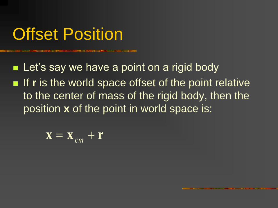
Offset Position

Let’s say we have a point on a rigid body

If r is the world space offset of the point relative

to the center of mass of the rigid body, then the

position x of the point in world space is:

rxx cm

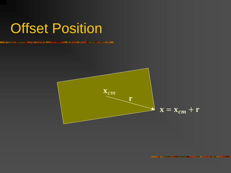
Offset Position

𝐱𝑐𝑚 𝐫

𝐱 = 𝐱𝒄𝒎 + 𝐫

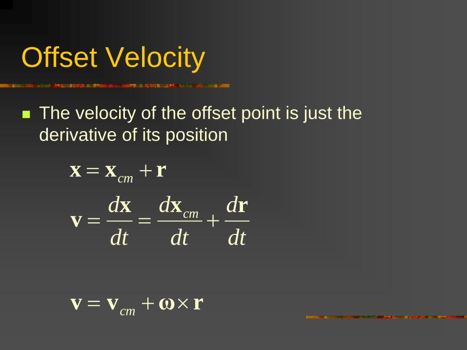
Offset Velocity

The velocity of the offset point is just the

derivative of its position

rωvv

rxxv

rxx

cm

cm

cm

dt

d

dt

d

dt

d

Offset Acceleration

The offset acceleration is the derivative of the

offset velocity

rωωrωaa

rωr

ωvva

rωvv

cm

cm

cm

dt

d

dt

d

dt

d

dt

d

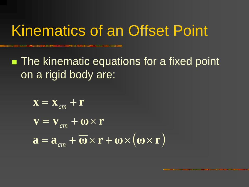
Kinematics of an Offset Point

The kinematic equations for a fixed point

on a rigid body are:

rωωrωaa

rωvv

rxx

cm

cm

cm

Inverse Mass Matrix

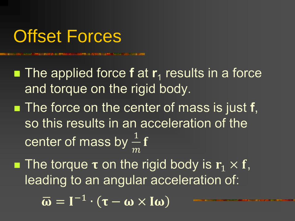
Offset Forces

Suppose we have a particle

If we apply a force to it, what is the

resulting acceleration?

Easy:

Offset Forces

With rigid bodies, the same holds true for

the acceleration of the center of mass

However, what if we’re interested in the

acceleration of some offset point?

If we apply a force f to a rigid body at

offset r1, what is the resulting acceleration

at a (possibly) different offset r2?

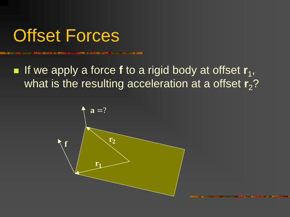
Offset Forces

𝐟

𝐚 =?

𝐫𝟏

𝐫𝟐

If we apply a force f to a rigid body at offset r1,

what is the resulting acceleration at a offset r2?

Offset Forces

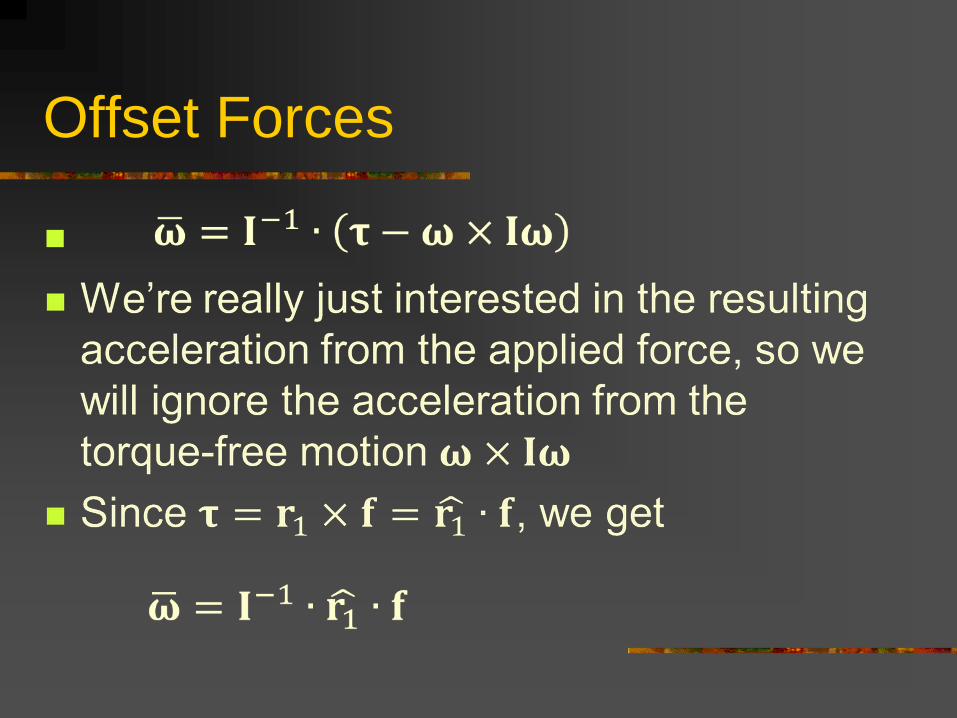
Offset Forces

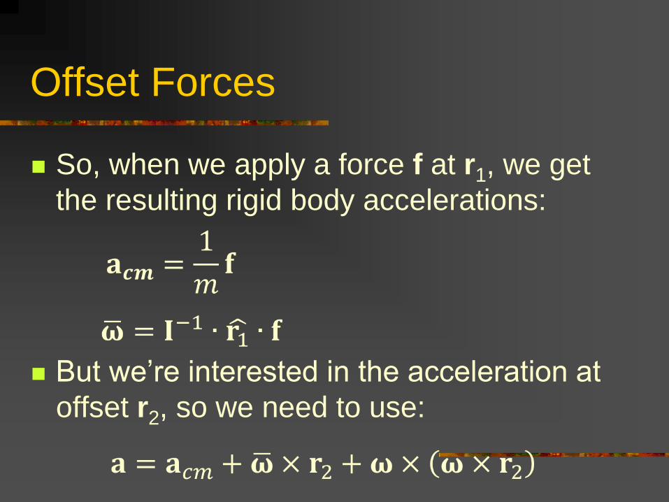
Offset Forces

So, when we apply a force f at r1, we get

the resulting rigid body accelerations:

But we’re interested in the acceleration at

offset r2, so we need to use:

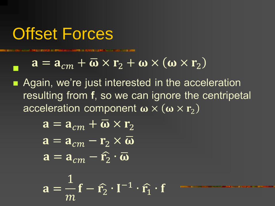
Offset Forces

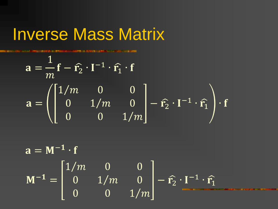
Inverse Mass Matrix

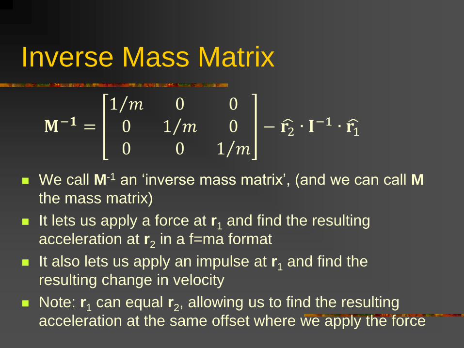
Inverse Mass Matrix

We call M-1 an ‘inverse mass matrix’, (and we can call M

the mass matrix)

It lets us apply a force at r1 and find the resulting

acceleration at r2 in a f=ma format

It also lets us apply an impulse at r1 and find the

resulting change in velocity

Note: r1 can equal r2, allowing us to find the resulting

acceleration at the same offset where we apply the force

Inverse Mass Matrix

Why do we care?

Well, this lets us do all kinds of useful things

such as collisions and constraints

For a collision, for example, we can use it to

solve what impulse will prevent the velocity of a

colliding point to go through another object

For a constraint, we can solve the constraint

force the holds an offset point still (zero

acceleration)

Collisions & Constraints

Collisions

Lets say we have a rigid body that hits the ground at

offset point r

We will assume the collision has zero elasticity and high

enough friction to zero out any tangential velocity

The velocity at the collision point is

The collision will result in an impulse that causes the

offset velocity v to go to zero immediately after the

collision

Therefore, we want to solve for impulse j:

Collisions

There’s a lot more to say about collisions

For starters, that example was of one rigid body colliding

with an infinite mass and we’ll need to have rigid bodies

colliding with other rigid bodies

Also, we want to handle non-zero elasticity, and a

realistic friction model

Then comes issues of multiple simultaneous collisions

Then static contact situations…

Then rolling and sliding…

Then stacking…

Constraints

It is common to add constraints to a rigid body system that allows us

to create articulated figures with various joint types

For example, we could constrain an offset position of one rigid body

to match a different offset position on another rigid body, thus

creating a ball-and-socket type joint

The constraint would apply some force to the first rigid body and an

equal an opposite force to the second. The constraint force would

be whatever force is necessary to keep the two points from

separating

We can use the inverse mass matrix technique to formulate an

equation that lets us solve for the unknown constraint force

If multiple objects are constrained together in a large group, then we

must simultaneously solve for all of these constraint forces in one

big system of equations

Constraints & Collisions

It turns out that constraints and collisions can be formulated in very

similar ways although there are some important differences

(namely, constraints form equality equations and collisions form

inequality equations)

They can all be included in one big system and then solved by a

special inequality solver called an LCP solver (LCP stands for linear

complementarity problem) or by other techniques

This lets us combine rigid body motion, constraints, and collisions

into one single process

The details are outside the scope of this class, but I’ve included a

pdf on the web page that gives an overview of the state of the art in

rigid body simulation