1

PHY 564 Fall 2015 Lecture 3

PHY 564 Advanced Accelerator Physics

Lecture 6

Vladimir N. Litvinenko Yichao Jing Gang Wang

Department of Physics & Astronomy, Stony Brook University

Collider-Accelerator Department, Brookhaven National Laboratory

2

Recap of previous lecture

3

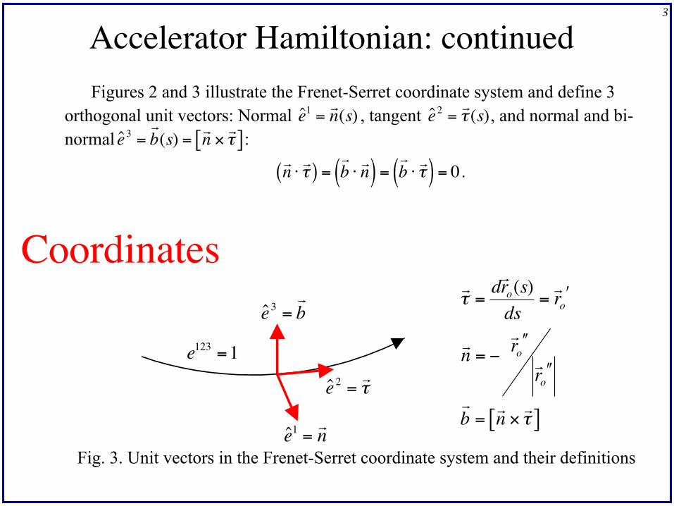
Accelerator Hamiltonian: continuedFigures 2 and 3 illustrate the Frenet-Serret coordinate system and define 3

orthogonal unit vectors: Normal

€

ˆ e 1 =! n (s) , tangent

€

ˆ e 2 =! τ (s), and normal and bi-

normal

€

ˆ e 3 =! b (s) =

! n × ! τ [ ] :

€

! n ⋅ ! τ ( ) =! b ⋅ ! n ( ) =

! b ⋅ ! τ ( ) = 0 .

€

ˆ e 3 = b

€

ˆ e 2 = τ

€

ˆ e 1 = n

€

τ =

d r o(s)ds

= r o#

n = −

r o## r o##

b = n × τ [ ]€

e123 =1

Fig. 3. Unit vectors in the Frenet-Serret coordinate system and their definitions

Coordinates

4

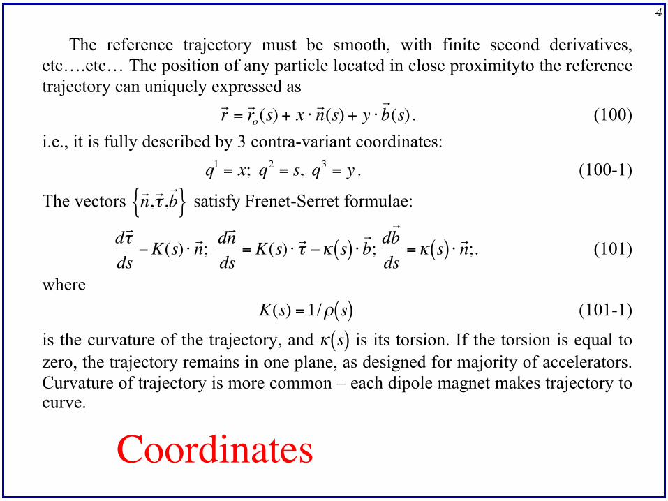
The reference trajectory must be smooth, with finite second derivatives, etc….etc… The position of any particle located in close proximityto the reference trajectory can uniquely expressed as

€

! r =! r o(s) + x ⋅

! n (s) + y ⋅

! b (s) . (100)

i.e., it is fully described by 3 contra-variant coordinates:

€

q1 = x; q2 = s, q3 = y . (100-1)

The vectors

€

! n , ! τ ,! b { } satisfy Frenet-Serret formulae:

€

d! τ ds

−K(s) ⋅ ! n ; d! n ds

= K(s) ⋅ ! τ −κ s( ) ⋅! b ; d! b

ds=κ s( ) ⋅

! n ;. (101)

where

€

K(s) =1/ρ s( ) (101-1)

is the curvature of the trajectory, and

€

κ s( ) is its torsion. If the torsion is equal to zero, the trajectory remains in one plane, as designed for majority of accelerators. Curvature of trajectory is more common – each dipole magnet makes trajectory to curve.

Coordinates

5

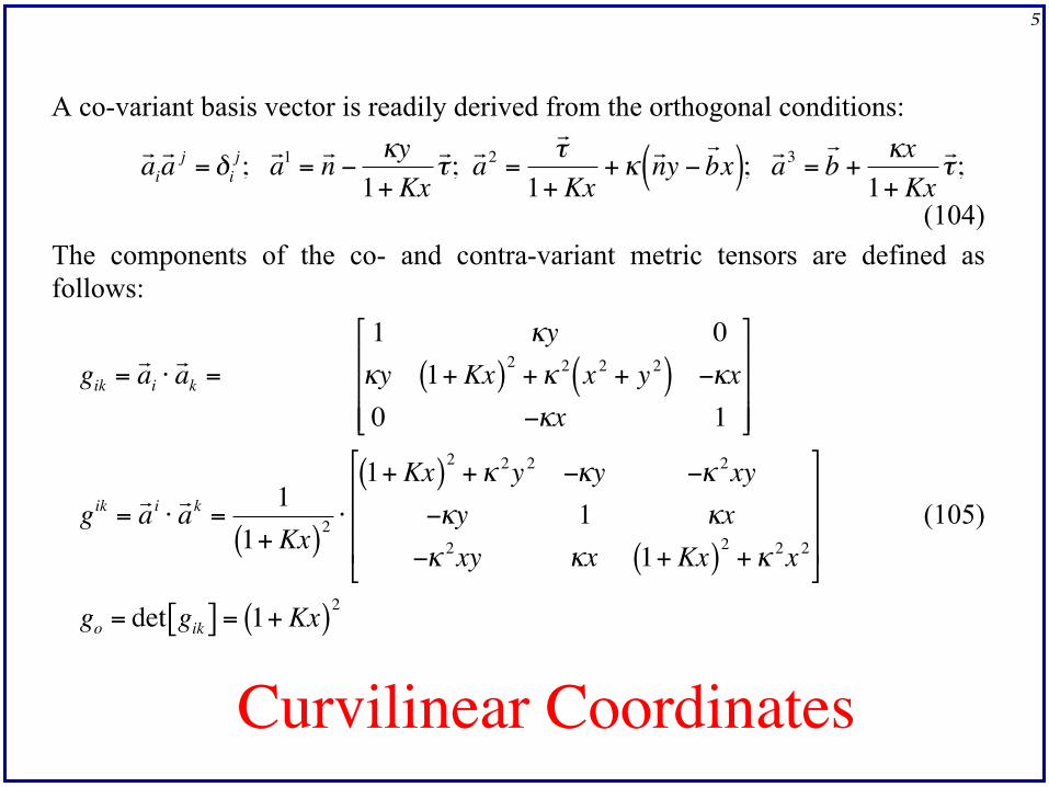
A co-variant basis vector is readily derived from the orthogonal conditions:

€

! a i! a j = δi

j; ! a 1 =! n − κy

1+ Kx! τ ; ! a 2 =

! τ

1+ Kx+κ! n y −! b x( ); ! a 3 =

! b + κx

1+ Kx! τ ;

(104) The components of the co- and contra-variant metric tensors are defined as follows:

€

gik =! a i ⋅! a k =

1 κy 0κy 1+ Kx( )2

+κ 2 x 2 + y 2( ) −κx0 −κx 1

%

&

' ' '

(

)

* * *

gik =! a i ⋅! a k =

11+ Kx( )2 ⋅

1+ Kx( )2+κ 2y 2 −κy −κ 2xy

−κy 1 κx−κ 2xy κx 1+ Kx( )2

+κ 2x 2

%

&

' ' '

(

)

* * *

go = det gik[ ] = 1+ Kx( )2

(105)

Curvilinear Coordinates

6

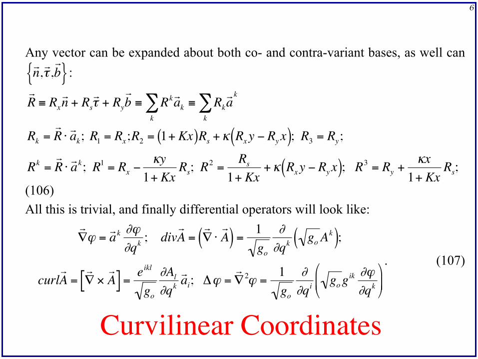
Any vector can be expanded about both co- and contra-variant bases, as well can

€

! n , ! τ ,! b { } :

€

! R ≡ Rx

! n + Rs

! τ + Ry

! b ≡ Rk ! a k

k∑ ≡ Rk

! a

k∑

k

Rk =! R ⋅! a k; R1 = Rx;R2 = 1+ Kx( )Rs +κ Rx y − Ry x( ); R3 = Ry;

Rk =! R ⋅! a k; R1 = Rx −

κy1+ Kx

Rs; R2 =Rs

1+ Kx+κ Rx y − Ry x( ); R3 = Ry +

κx1+ Kx

Rs;

(106) All this is trivial, and finally differential operators will look like:

€

! ∇ ϕ =

! a k ∂ϕ∂qk ; div

! A =

! ∇ ⋅! A ( ) =

1go

∂∂qk go Ak( );

curl! A =

! ∇ ×! A [ ] =

eikl

go

∂Al

∂qk

! a i; Δϕ =

! ∇ 2ϕ =

1go

∂∂qi go gik ∂ϕ

∂qk

(

) *

+

, -

. (107)

Curvilinear Coordinates

7

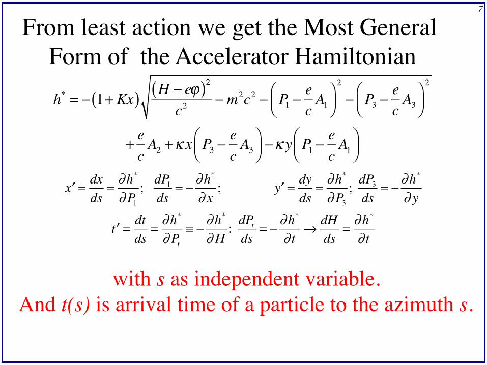
h* = − 1+ Kx( ) H − eϕ( )2c2

−m2c2 − P1 −ecA1

⎛⎝⎜

⎞⎠⎟2

− P3 −ecA3

⎛⎝⎜

⎞⎠⎟2

+ ecA2 +κ x P3 −

ecA3

⎛⎝⎜

⎞⎠⎟ −κ y P1 −

ecA1

⎛⎝⎜

⎞⎠⎟

′x = dxds

= ∂h*

∂P1

; dP1

ds= − ∂h

*

∂ x; ′y = dy

ds= ∂h*

∂P3

; dP3

ds= − ∂h

*

∂ y

′t = dtds

= ∂h*

∂Pt≡ − ∂h

*

∂H; dPtds

= − ∂h*

∂ t→ dH

ds= ∂h*

∂ t

From least action we get the Most General Form of the Accelerator Hamiltonian

with s as independent variable.And t(s) is arrival time of a particle to the azimuth s.

8

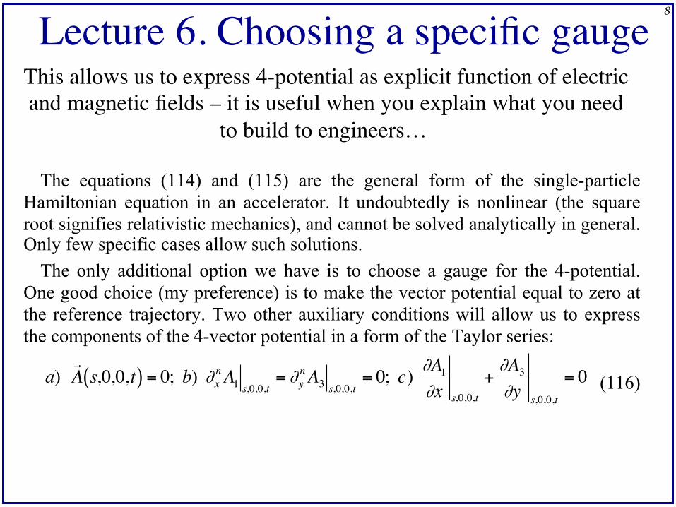
Lecture 6. Choosing a specific gaugeThis allows us to express 4-potential as explicit function of electric and magnetic fields – it is useful when you explain what you need

to build to engineers…

The equations (114) and (115) are the general form of the single-particle Hamiltonian equation in an accelerator. It undoubtedly is nonlinear (the square root signifies relativistic mechanics), and cannot be solved analytically in general. Only few specific cases allow such solutions.

The only additional option we have is to choose a gauge for the 4-potential. One good choice (my preference) is to make the vector potential equal to zero at the reference trajectory. Two other auxiliary conditions will allow us to express the components of the 4-vector potential in a form of the Taylor series:

€

a) ! A s,0,0,t( ) = 0; b) ∂x

n A1 s,0,0,t= ∂y

n A3 s,0,0,t= 0; c) ∂A1

∂x s,0,0,t

+∂A3

∂y s,0,0,t

= 0 (116)

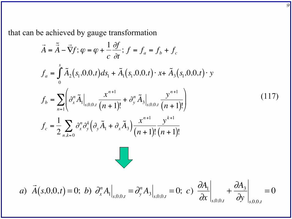
9

that can be achieved by gauge transformation

€

! A =! ˜ A −! ∇ f ;ϕ =ϕ +

1c∂f∂t

; f = fa = fb + fc

fa = ˜ A 2 s1,0,0,t( )ds10

s

∫ + ˜ A 1 s1,0,0,t( ) ⋅ x+ ˜ A 3 s1,0,0,t( ) ⋅ y

fb = ∂xn ˜ A 1 s,0,0,t

x n +1

n +1( )!+ ∂y

n ˜ A 3 s,0,0,t

y n +1

n +1( )!(

) *

+

, -

n=1∑

fc =12

∂xn∂y

k ∂y˜ A 1 + ∂x

˜ A 3( ) xn +1

n +1( )!yk +1

n +1( )!n,k= 0∑

(117)

�

a) ! A s,0,0,t( ) = 0; b) ∂x

n A1 s,0,0,t= ∂y

n A3 s,0,0,t= 0; c) ∂A1

∂x s,0,0,t

+ ∂A3

∂y s,0,0,t

= 0

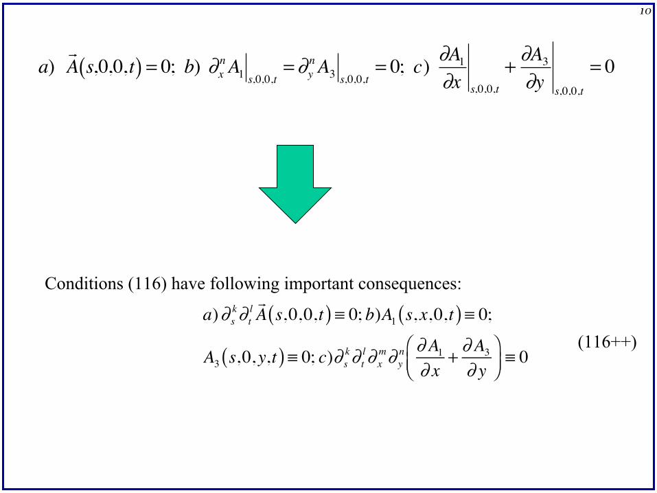
10

Conditions (116) have following important consequences:

a) ∂sk∂t

l!A s,0,0,t( ) ≡ 0; b)A1 s, x,0,t( ) ≡ 0;

A3 s,0, y,t( ) ≡ 0; c)∂sk∂t

l∂xm∂y

n ∂A1

∂ x+ ∂A3

∂ y⎛⎝⎜

⎞⎠⎟≡ 0

(116++)

�

a) ! A s,0,0,t( ) = 0; b) ∂x

n A1 s,0,0,t= ∂y

n A3 s,0,0,t= 0; c) ∂A1

∂x s,0,0,t

+ ∂A3

∂y s,0,0,t

= 0

11

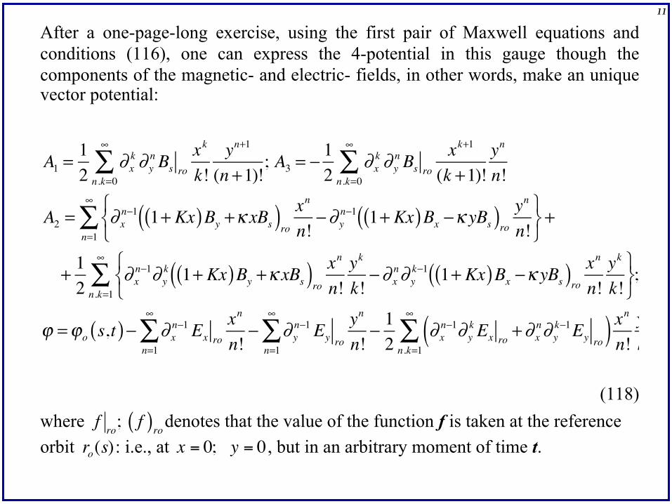
After a one-page-long exercise, using the first pair of Maxwell equations and conditions (116), one can express the 4-potential in this gauge though the components of the magnetic- and electric- fields, in other words, make an unique vector potential:

A1 =12

∂xk

n.k=0

∞

∑ ∂yn Bs ro

xk

k!yn+1

(n +1)!; A3 = − 1

2∂xk

n.k=0

∞

∑ ∂yn Bs ro

xk+1

(k +1)!yn

n!

A2 = ∂xn−1 1+ Kx( )By +κ xBs( )ro

xn

n!−∂y

n−1 1+ Kx( )Bx −κ yBs( )royn

n!⎧⎨⎩

⎫⎬⎭n=1

∞

∑ +

+ 12

∂xn−1∂y

k 1+ Kx( )By +κ xBs( )roxn

n!yk

k!−∂x

n∂yk−1 1+ Kx( )Bx −κ yBs( )ro

xn

n!yk

k!⎧⎨⎩

⎫⎬⎭n.k=1

∞

∑ ;

ϕ =ϕo s,t( )− ∂xn−1

n=1

∞

∑ Ex ro

xn

n!− ∂y

n−1

n=1

∞

∑ Ey ro

yn

n!− 1

2∂xn−1∂y

k Ex ro+ ∂x

n∂yk−1Ey ro( )

n.k=1

∞

∑ xn

n!yk

k!;

(118) where

€

f ro; f( )rodenotes that the value of the function f is taken at the reference orbit

€

ro(s): i.e., at

€

x = 0; y = 0 , but in an arbitrary moment of time t.

12

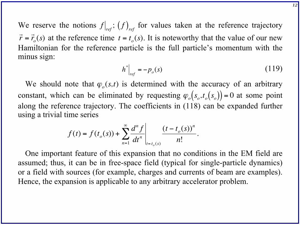
We reserve the notions

€

f ref ; f( )ref for values taken at the reference trajectory

€

! r =! r o(s) at the reference time

€

t = to(s). It is noteworthy that the value of our new Hamiltonian for the reference particle is the full particle’s momentum with the minus sign:

€

h*ref

= −po(s) (119)

We should note that

€

ϕo(s,t) is determined with the accuracy of an arbitrary constant, which can be eliminated by requesting

€

ϕo so,to so( )( ) = 0 at some point along the reference trajectory. The coefficients in (118) can be expanded further using a trivial time series

€

f (t) = f (to(s)) +dn fdt n t= to (s)

(t − to(s))n

n!n=1

∞

∑ .

One important feature of this expansion that no conditions in the EM field are assumed; thus, it can be in free-space field (typical for single-particle dynamics) or a field with sources (for example, charges and currents of beam are examples). Hence, the expansion is applicable to any arbitrary accelerator problem.

13

An equilibrium particle and a reference trajectory.

A particle that follows the reference trajectory is called an equilibrium (or reference) one:

�

! r =! r o(s); t = to(s); H = Ho(s) = Eo(s) + ϕo(s,to(s)) , (120)

with

�

x ≡ 0; y ≡ 0; px ≡ 0;py ≡ 0. This is where condition (L2.20a)

�

! A

ref= 0 is

useful, i.e., for

�

x ref = 0; y ref = 0; P1ref

= px ref + ecA1 ref ≡ 0; P3 ref = py ref

+ ecA3 ref ≡ 0. (121)

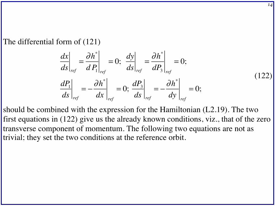
14

The differential form of (121)

dxds ref

= ∂h*

d P1 ref

= 0; dyds ref

= ∂h*

dP3 ref

= 0;

dP1

ds ref

= − ∂h*

dx ref

= 0; dP3

ds ref

= − ∂h*

dy ref

= 0; (122)

should be combined with the expression for the Hamiltonian (L2.19). The two first equations in (122) give us the already known conditions, viz., that of the zero transverse component of momentum. The following two equations are not as trivial; they set the two conditions at the reference orbit.

15

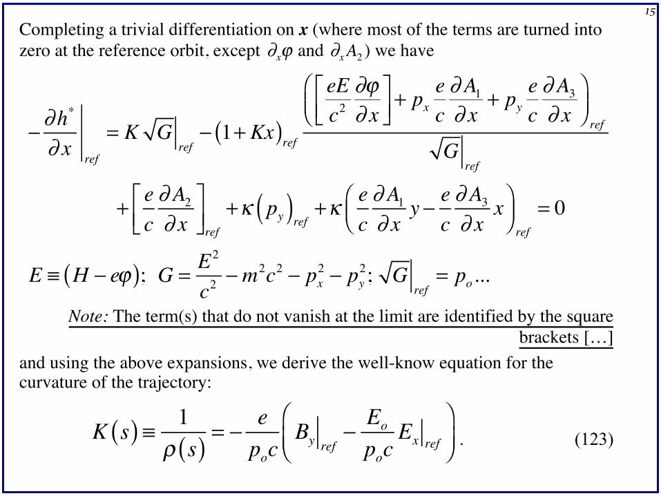
Completing a trivial differentiation on x (where most of the terms are turned into zero at the reference orbit, except

�

∂xϕ and

�

∂xA2 ) we have

− ∂h*

∂ x ref

= K Gref− 1+ Kx( )ref

eEc2

∂ϕ∂ x

⎡⎣⎢

⎤⎦⎥+ px

ec∂A1∂ x

+ pyec∂A3∂ x

⎛⎝⎜

⎞⎠⎟ ref

Gref

+ ec∂A2∂ x

⎡⎣⎢

⎤⎦⎥ref

+κ py( )ref +κec∂A1∂ x

y − ec∂A3∂ x

x⎛⎝⎜

⎞⎠⎟ ref

= 0

E ≡ H − eϕ( ); G = E2

c2−m2c2 − px

2 − py2; G

ref= po...

Note: The term(s) that do not vanish at the limit are identified by the square brackets […]

and using the above expansions, we derive the well-know equation for the curvature of the trajectory:

K s( ) ≡ 1ρ s( ) = − e

pocBy ref

− Eo

pocEx ref

⎛⎝⎜

⎞⎠⎟ . (123)

16

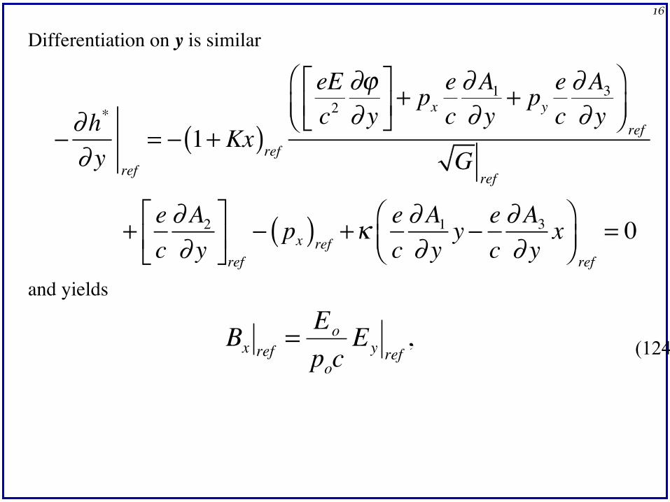
Differentiation on y is similar

− ∂h*

∂ y ref

= − 1+ Kx( )ref

eEc2

∂ϕ∂ y

⎡⎣⎢

⎤⎦⎥+ px

ec∂A1∂ y

+ pyec∂A3∂ y

⎛⎝⎜

⎞⎠⎟ ref

Gref

+ ec∂A2∂ y

⎡⎣⎢

⎤⎦⎥ref

− px( )ref +κec∂A1∂ y

y − ec∂A3∂ y

x⎛⎝⎜

⎞⎠⎟ ref

= 0

and yields

�

Bx ref = Eo

pocEy ref

, (124)

17

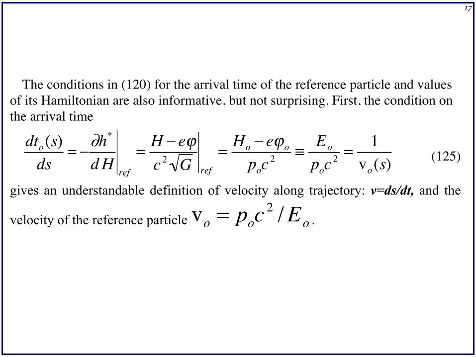
The conditions in (120) for the arrival time of the reference particle and values of its Hamiltonian are also informative, but not surprising. First, the condition on the arrival time

�

dto(s)ds

= −∂h*

dH ref

= H − eϕc 2 G ref

= Ho − eϕo

poc2 ≡ Eo

poc2 = 1

vo(s) (125)

gives an understandable definition of velocity along trajectory: v=ds/dt, and the

velocity of the reference particle

�

vo = poc2 /Eo .

18

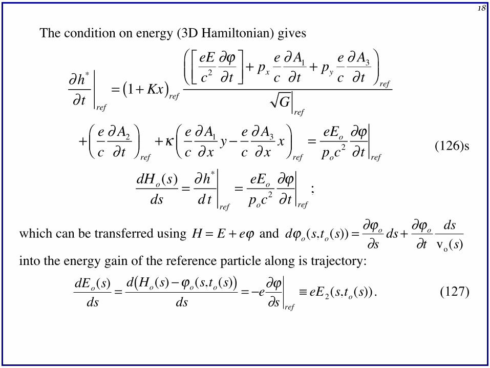
The condition on energy (3D Hamiltonian) gives

∂h*

∂ t ref

= 1+ Kx( )ref

eEc2

∂ϕ∂ t

⎡⎣⎢

⎤⎦⎥+ px

ec∂A1

∂ t+ py

ec∂A3

∂ t⎛⎝⎜

⎞⎠⎟ ref

Gref

+ ec∂A2

∂ t⎛⎝⎜

⎞⎠⎟ ref

+κ ec∂A1

∂ xy − e

c∂A3

∂ xx⎛

⎝⎜⎞⎠⎟ ref

= eEo

poc2∂ϕ∂ t ref

dHo(s)ds

= ∂h*

d tref

= eEo

poc2∂ϕ∂ t ref

;

(126)s

which can be transferred using

�

H = E + eϕ and

�

dϕo(s,to(s)) = ∂ϕo

∂sds+ ∂ϕo

∂tdsvo(s)

into the energy gain of the reference particle along is trajectory:

�

dEo(s)ds

=d Ho(s) −ϕo(s,to(s)( )

ds= −e∂ϕ

∂s ref

≡ eE2(s,to(s)) . (127)

19

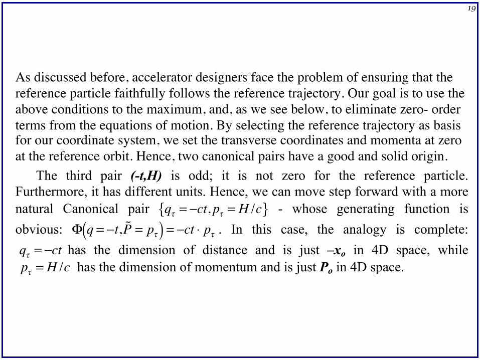
As discussed before, accelerator designers face the problem of ensuring that the reference particle faithfully follows the reference trajectory. Our goal is to use the above conditions to the maximum, and, as we see below, to eliminate zero- order terms from the equations of motion. By selecting the reference trajectory as basis for our coordinate system, we set the transverse coordinates and momenta at zero at the reference orbit. Hence, two canonical pairs have a good and solid origin.

The third pair (-t,H) is odd; it is not zero for the reference particle. Furthermore, it has different units. Hence, we can move step forward with a more natural Canonical pair

�

qτ = −ct, pτ = H /c{ } - whose generating function is obvious:

�

Φ q = −t, ˜ P = pτ( ) = −ct ⋅ pτ . In this case, the analogy is complete:

�

qτ = −ct has the dimension of distance and is just –xo in 4D space, while

�

pτ = H /c has the dimension of momentum and is just Po in 4D space.

20

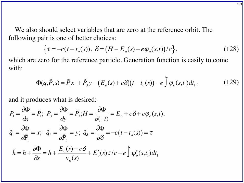
We also should select variables that are zero at the reference orbit. The following pair is one of better choices:

�

τ = −c(t − to(s)), δ = H − Eo(s) − eϕo(s,t)( ) /c{ }, (128) which are zero for the reference particle. Generation function is easily to come with:

�

Φ(q, ˜ P ,s) = ˜ P 1x + ˜ P 3y − Eo(s) + cδ( ) t − to(s)( ) − e ϕo(s,t1)dt1t

∫ , (129)

and it produces what is desired:

�

P1 = ∂Φ∂x

= ˜ P 1; P3 = ∂Φ∂y

= ˜ P 3;H = ∂Φ∂(−t)

= Eo + cδ + eϕo(s,t);

˜ q 1 = ∂Φ∂ ˜ P 1

= x; ˜ q 3 = ∂Φ∂ ˜ P 3

= y; ˜ q δ = ∂Φ∂δ

= −c t − to(s)( ) = τ

˜ h = h + ∂Φ∂s

= h + Eo(s) + cδvo(s)

+ ′ E o(s)τ /c − e ′ ϕ o(s,t1)dt1t

∫

21

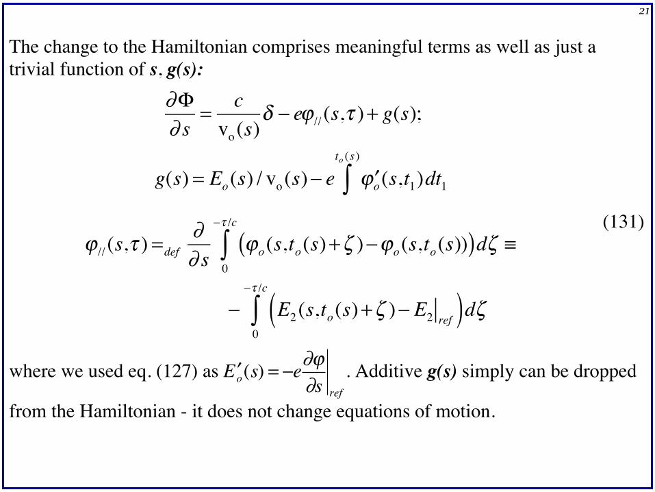
The change to the Hamiltonian comprises meaningful terms as well as just a trivial function of s, g(s):

∂Φ∂ s

= cvo(s)

δ − eϕ // (s,τ )+ g(s);

g(s) = Eo(s) / vo(s)− e ′ϕo(s,t1)dt1to (s )

∫

ϕ // (s,τ ) =def∂∂ s

ϕo(s,to(s)+ζ )−ϕo(s,to(s))( )dζ0

−τ /c

∫ ≡

− E2 (s,to(s)+ζ )− E2 ref( )dζ0

−τ /c

∫

(131)

where we used eq. (127) as

�

′ E o(s) = −e∂ϕ∂s ref

. Additive g(s) simply can be dropped

from the Hamiltonian - it does not change equations of motion.

22

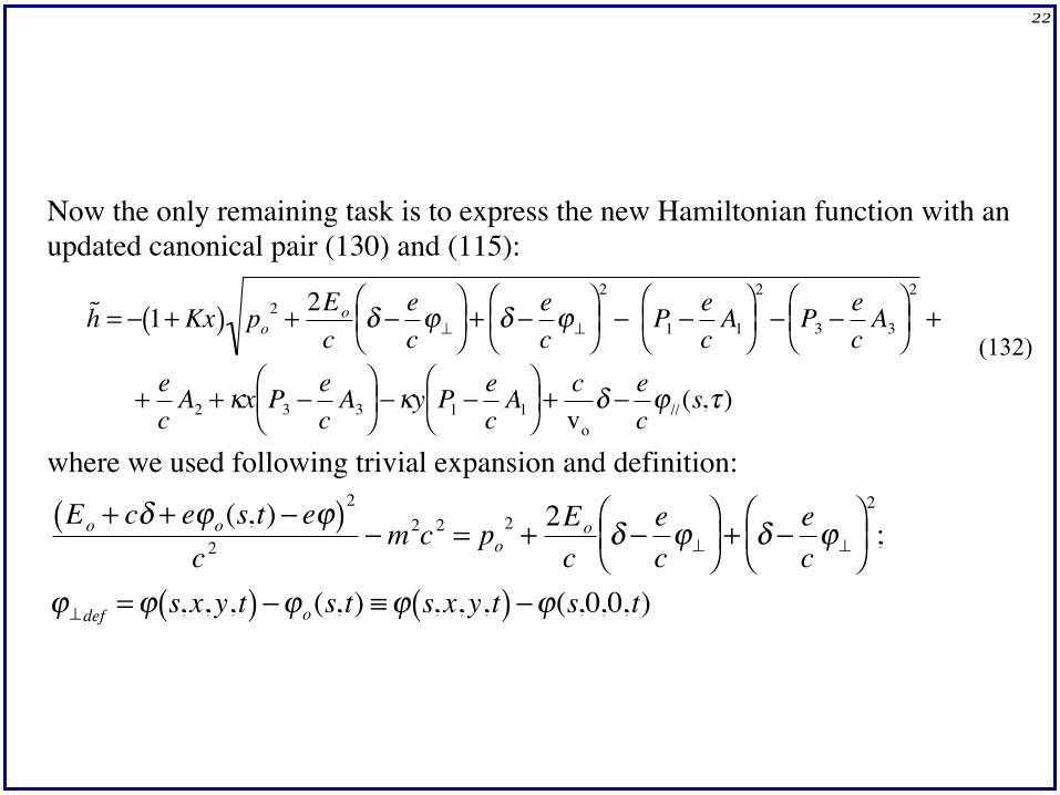
Now the only remaining task is to express the new Hamiltonian function with an updated canonical pair (130) and (115):

�

˜ h = − 1+ Kx( ) po2 + 2Eo

cδ − e

cϕ⊥

⎛ ⎝ ⎜

⎞ ⎠ ⎟ + δ − e

cϕ⊥

⎛ ⎝ ⎜

⎞ ⎠ ⎟

2

− P1 −ec

A1⎛ ⎝ ⎜

⎞ ⎠ ⎟

2

− P3 −ec

A3⎛ ⎝ ⎜

⎞ ⎠ ⎟

2

+

+ ec

A2 + κx P3 −ec

A3⎛ ⎝ ⎜

⎞ ⎠ ⎟ −κy P1 −

ec

A1⎛ ⎝ ⎜

⎞ ⎠ ⎟ +

cvo

δ − ecϕ // (s,τ )

(132)

where we used following trivial expansion and definition:

�

Eo + cδ + eϕo(s,t) − eϕ( )2c 2

−m2c 2 = po2 + 2Eo

cδ − e

cϕ⊥

⎛ ⎝ ⎜

⎞ ⎠ ⎟ + δ − e

cϕ⊥

⎛ ⎝ ⎜

⎞ ⎠ ⎟ 2

;

ϕ⊥def = ϕ s,x,y,t( ) −ϕo(s,t) ≡ϕ s,x,y,t( ) −ϕ(s,0,0,t)

23

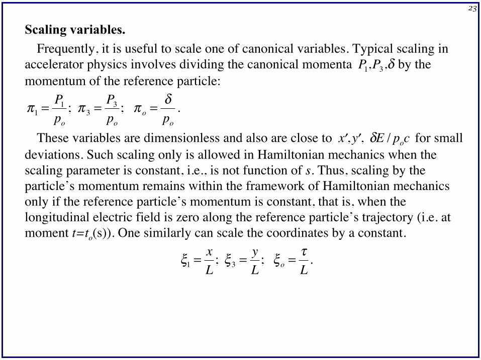
Scaling variables. Frequently, it is useful to scale one of canonical variables. Typical scaling in

accelerator physics involves dividing the canonical momenta

�

P1,P3,δ by the momentum of the reference particle:

�

π1 = P1

po; π 3 = P3

po; π o = δ

po. (134)

These variables are dimensionless and also are close to

�

′ x , ′ y , δE / poc for small deviations. Such scaling only is allowed in Hamiltonian mechanics when the scaling parameter is constant, i.e., is not function of s. Thus, scaling by the particle’s momentum remains within the framework of Hamiltonian mechanics only if the reference particle’s momentum is constant, that is, when the longitudinal electric field is zero along the reference particle’s trajectory (i.e. at moment t=to(s)). One similarly can scale the coordinates by a constant.

�

ξ1 = xL

; ξ3 = yL

; ξo = τL

.

24

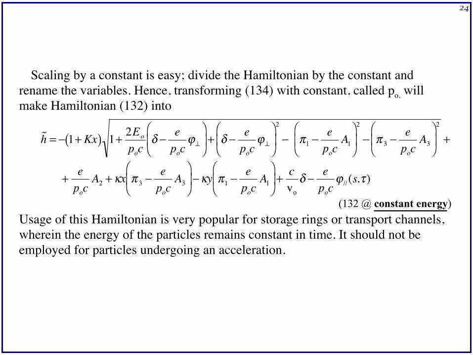
Scaling by a constant is easy; divide the Hamiltonian by the constant and rename the variables. Hence, transforming (134) with constant, called po, will make Hamiltonian (132) into

�

˜ h = − 1+ Kx( ) 1+ 2Eo

pocδ − e

pocϕ⊥

⎛

⎝ ⎜

⎞

⎠ ⎟ + δ − e

pocϕ⊥

⎛

⎝ ⎜

⎞

⎠ ⎟

2

− π1 −e

pocA1

⎛

⎝ ⎜

⎞

⎠ ⎟

2

− π 3 −e

pocA3

⎛

⎝ ⎜

⎞

⎠ ⎟

2

+

+ epoc

A2 + κx π 3 −e

pocA3

⎛

⎝ ⎜

⎞

⎠ ⎟ −κy π1 −

epoc

A1

⎛

⎝ ⎜

⎞

⎠ ⎟ +

cvo

δ − epoc

ϕ // (s,τ )

(132 @ constant energy) Usage of this Hamiltonian is very popular for storage rings or transport channels, wherein the energy of the particles remains constant in time. It should not be employed for particles undergoing an acceleration.

25

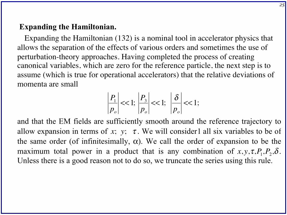
Expanding the Hamiltonian. Expanding the Hamiltonian (132) is a nominal tool in accelerator physics that

allows the separation of the effects of various orders and sometimes the use of perturbation-theory approaches. Having completed the process of creating canonical variables, which are zero for the reference particle, the next step is to assume (which is true for operational accelerators) that the relative deviations of momenta are small

�

P1

po<< 1; P3

po<< 1; δ

po<< 1;

and that the EM fields are sufficiently smooth around the reference trajectory to allow expansion in terms of

�

x; y; τ . We will consider1 all six variables to be of the same order (of infinitesimally, α). We call the order of expansion to be the maximum total power in a product that is any combination of

�

x,y,τ,P1,P2,δ . Unless there is a good reason not to do so, we truncate the series using this rule.

1 Sometimes, one can keep explicit the time dependence of fields and expand only the rest of the variables. One such case is an approximate, and useful, description of synchrotron oscillation.

26

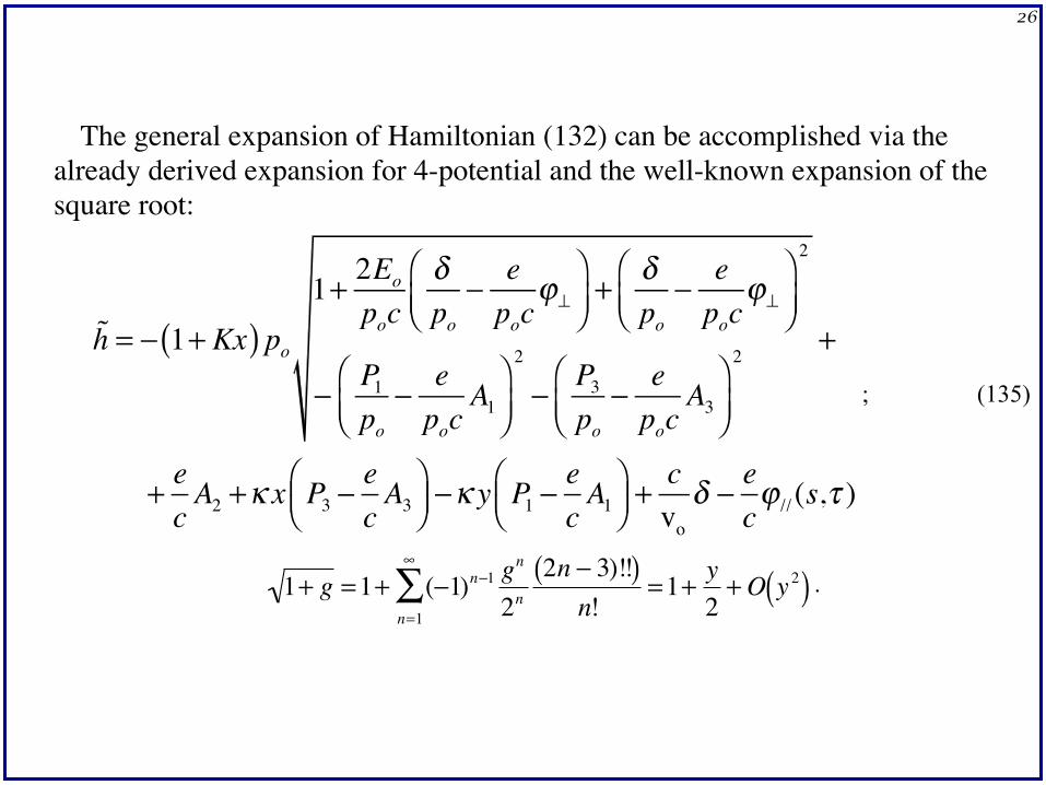
The general expansion of Hamiltonian (132) can be accomplished via the already derived expansion for 4-potential and the well-known expansion of the square root:

!h = − 1+ Kx( ) po1+ 2Eo

pocδpo

− epoc

ϕ⊥⎛⎝⎜

⎞⎠⎟+ δ

po− epoc

ϕ⊥⎛⎝⎜

⎞⎠⎟

2

− P1

po− epoc

A1⎛⎝⎜

⎞⎠⎟

2

− P3

po− epoc

A3⎛⎝⎜

⎞⎠⎟

2+

+ ecA2 +κ x P3 −

ecA3

⎛⎝⎜

⎞⎠⎟ −κ y P1 −

ecA1

⎛⎝⎜

⎞⎠⎟ +

cvo

δ − ecϕ // (s,τ )

; (135)

�

1+ g =1+ (−1)n−1 gn

2nn=1

∞

∑ 2n − 3)!!( )n!

=1+ y2

+ O y 2( ) .

27

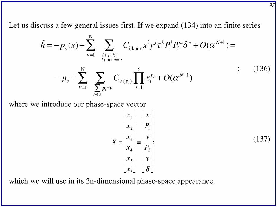
Let us discuss a few general issues first. If we expand (134) into an finite series

!h = − po(s)+ Cijklnmi+ j+k+l+m+n=ν

∑ν=1

Ν

∑ xiy jτ kP1lP3

mδ n +O(α N+1) =

− po + Cν { pi }pi

i=1,6∑ =ν∑

ν=1

Ν

∑ xipi

i=1

6

∏ +O(α N+1); (136)

where we introduce our phase-space vector

�

X =

x1x2x3x4x5x6

⎡

⎣

⎢ ⎢ ⎢ ⎢ ⎢ ⎢ ⎢

⎤

⎦

⎥ ⎥ ⎥ ⎥ ⎥ ⎥ ⎥

≡

xP1yP2τδ

⎡

⎣

⎢ ⎢ ⎢ ⎢ ⎢ ⎢ ⎢

⎤

⎦

⎥ ⎥ ⎥ ⎥ ⎥ ⎥ ⎥

; (137)

which we will use in its 2n-dimensional phase-space appearance.

28

�

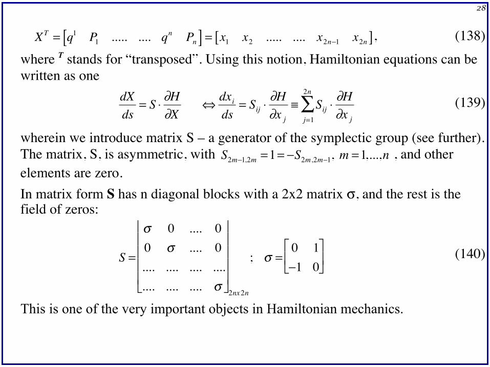
XT = q1 P1 ..... .... qn Pn[ ] = x1 x2 ..... .... x2n−1 x2n[ ], (138)

where T stands for “transposed”. Using this notion, Hamiltonian equations can be written as one

�

dXds

= S ⋅ ∂H∂X

⇔ dxids

= Sij ⋅∂H∂x j

≡ Sij ⋅∂H∂x jj=1

2n

∑ (139)

wherein we introduce matrix S – a generator of the symplectic group (see further). The matrix, S, is asymmetric, with

�

S2m−1,2m =1= −S2m,2m−1, m =1,...,n , and other elements are zero. In matrix form S has n diagonal blocks with a 2x2 matrix σ, and the rest is the field of zeros:

�

S =

σ 0 .... 00 σ .... 0.... .... .... ........ .... .... σ

⎡

⎣

⎢ ⎢ ⎢ ⎢

⎤

⎦

⎥ ⎥ ⎥ ⎥ 2nx2n

; σ =0 1−1 0⎡

⎣ ⎢

⎤

⎦ ⎥ (140)

This is one of the very important objects in Hamiltonian mechanics.

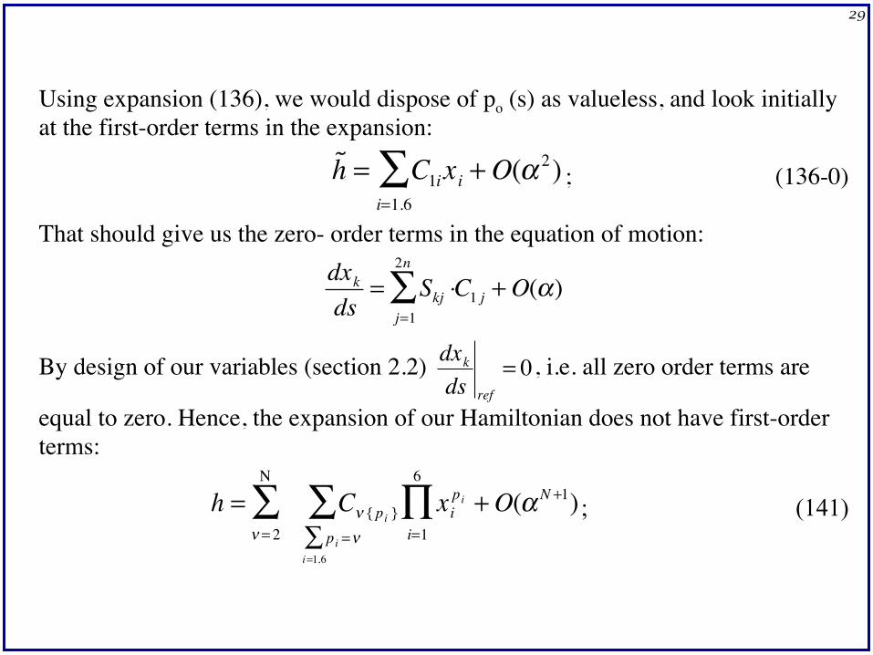
29

Using expansion (136), we would dispose of po (s) as valueless, and look initially at the first-order terms in the expansion:

�

˜ h = C1ii=1.6∑ xi + O(α 2) ; (136-0)

That should give us the zero- order terms in the equation of motion:

�

dxkds

= Skj ⋅j=1

2n

∑ C1 j + O(α)

By design of our variables (section 2.2)

�

dxkds ref

= 0, i.e. all zero order terms are

equal to zero. Hence, the expansion of our Hamiltonian does not have first-order terms:

�

h = Cν {pi }pi

i=1,6∑ =ν

∑ν = 2

Ν

∑ xipi

i=1

6

∏ + O(α N +1) ; (141)

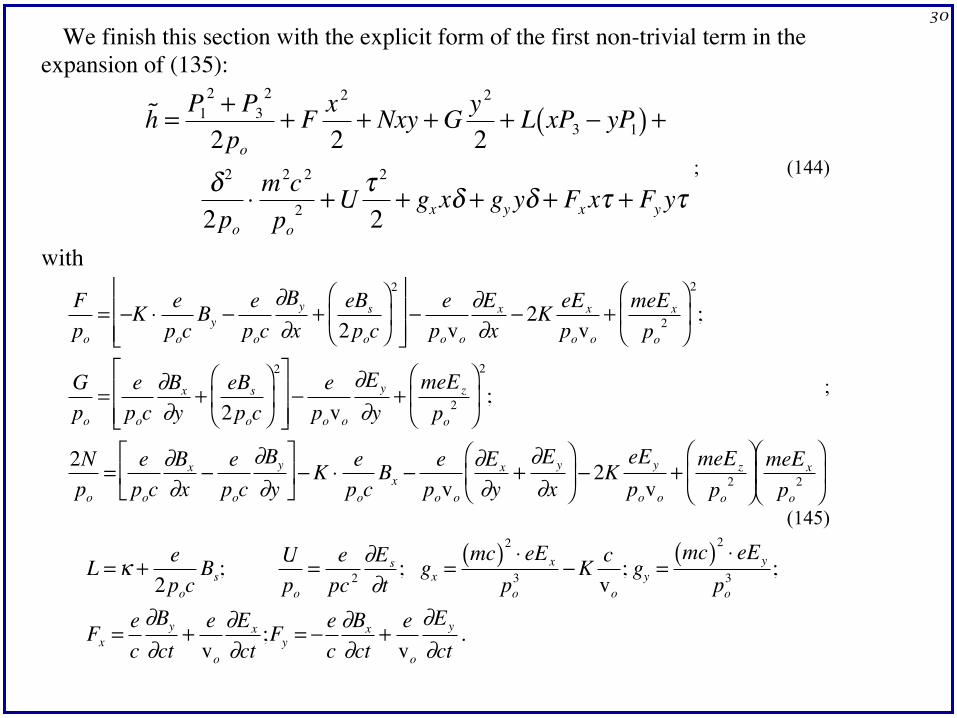
30 We finish this section with the explicit form of the first non-trivial term in the

expansion of (135):

�

˜ h = P12 + P3

2

2po

+ F x 2

2+ Nxy + G y 2

2+ L xP3 − yP1( ) +

δ 2

2po

⋅ m2c 2

po2 + U τ 2

2+ gx xδ + gy yδ + Fx xτ + Fy yτ

; (144)

with

�

Fpo

= −K ⋅ epoc

By −epoc

∂By

∂x+ eBs2poc⎛

⎝ ⎜

⎞

⎠ ⎟ 2⎡

⎣ ⎢ ⎢

⎤

⎦ ⎥ ⎥ − epovo

∂Ex

∂x− 2K eEx

povo+ meEx

po2

⎛

⎝ ⎜

⎞

⎠ ⎟ 2

;

Gpo

= epoc

∂Bx

∂y+ eBs

2poc⎛

⎝ ⎜

⎞

⎠ ⎟ 2⎡

⎣ ⎢ ⎢

⎤

⎦ ⎥ ⎥ − epovo

∂Ey

∂y+ meEz

po2

⎛

⎝ ⎜

⎞

⎠ ⎟ 2

;

2Npo

= epoc

∂Bx

∂x− epoc

∂By

∂y⎡

⎣ ⎢

⎤

⎦ ⎥ −K ⋅ e

pocBx −

epovo

∂Ex

∂y+∂Ey

∂x⎛

⎝ ⎜

⎞

⎠ ⎟ − 2K

eEy

povo+ meEz

po2

⎛

⎝ ⎜

⎞

⎠ ⎟ meEx

po2

⎛

⎝ ⎜

⎞

⎠ ⎟

;

(145)

�

L = κ + e2poc

Bs; Upo

= epc 2

∂Es

∂t; gx =

mc( )2 ⋅ eEx

po3 −K c

vo

; gy =mc( )2 ⋅ eEy

po3 ;

Fx = ec∂By

∂ct+ e

vo

∂Ex

∂ct;Fy = − e

c∂Bx

∂ct+ e

vo

∂Ey

∂ct.

31 We finish this section with the explicit form of the first non-trivial term in the

expansion of (135):

�

˜ h = P12 + P3

2

2po

+ F x 2

2+ Nxy + G y 2

2+ L xP3 − yP1( ) +

δ 2

2po

⋅ m2c 2

po2 + U τ 2

2+ gx xδ + gy yδ + Fx xτ + Fy yτ

; (143)

with

�

Fpo

= −K ⋅ epoc

By −epoc

∂By

∂x+ eBs2poc⎛

⎝ ⎜

⎞

⎠ ⎟ 2⎡

⎣ ⎢ ⎢

⎤

⎦ ⎥ ⎥ − epovo

∂Ex

∂x− 2K eEx

povo+ meEx

po2

⎛

⎝ ⎜

⎞

⎠ ⎟ 2

;

Gpo

= epoc

∂Bx

∂y+ eBs

2poc⎛

⎝ ⎜

⎞

⎠ ⎟ 2⎡

⎣ ⎢ ⎢

⎤

⎦ ⎥ ⎥ − epovo

∂Ey

∂y+ meEz

po2

⎛

⎝ ⎜

⎞

⎠ ⎟ 2

;

2Npo

= epoc

∂Bx

∂x− epoc

∂By

∂y⎡

⎣ ⎢

⎤

⎦ ⎥ −K ⋅ e

pocBx −

epovo

∂Ex

∂y+∂Ey

∂x⎛

⎝ ⎜

⎞

⎠ ⎟ − 2K

eEy

povo+ meEz

po2

⎛

⎝ ⎜

⎞

⎠ ⎟ meEx

po2

⎛

⎝ ⎜

⎞

⎠ ⎟

;

(144)

�

L = κ + e2poc

Bs; Upo

= epc 2

∂Es

∂t; gx =

mc( )2 ⋅ eEx

po3 −K c

vo

; gy =mc( )2 ⋅ eEy

po3 ;

Fx = ec∂By

∂ct+ e

vo

∂Ex

∂ct;Fy = − e

c∂Bx

∂ct+ e

vo

∂Ey

∂ct.

32

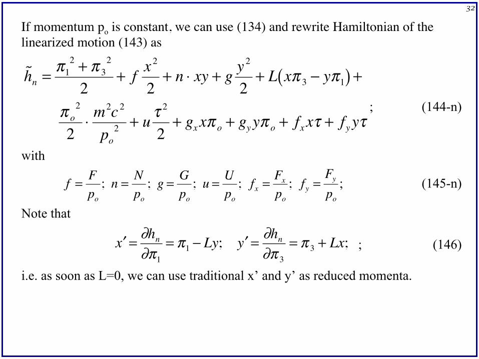
If momentum po is constant, we can use (134) and rewrite Hamiltonian of the linearized motion (143) as

�

˜ h n = π12 + π 3

2

2+ f x 2

2+ n ⋅ xy + g y 2

2+ L xπ 3 − yπ1( ) +

π o2

2⋅ m2c 2

po2 + u τ

2

2+ gx xπ o + gy yπ o + fx xτ + fy yτ

; (144-n)

with

�

f = Fpo

; n = Npo

; g = Gpo

; u = Upo

; fx = Fxpo

; fy =Fypo

; (145-n)

Note that

�

′ x = ∂hn

∂π1

= π1 − Ly; ′ y = ∂hn

∂π 3

= π 3 + Lx; ; (146)

i.e. as soon as L=0, we can use traditional x’ and y’ as reduced momenta.

33

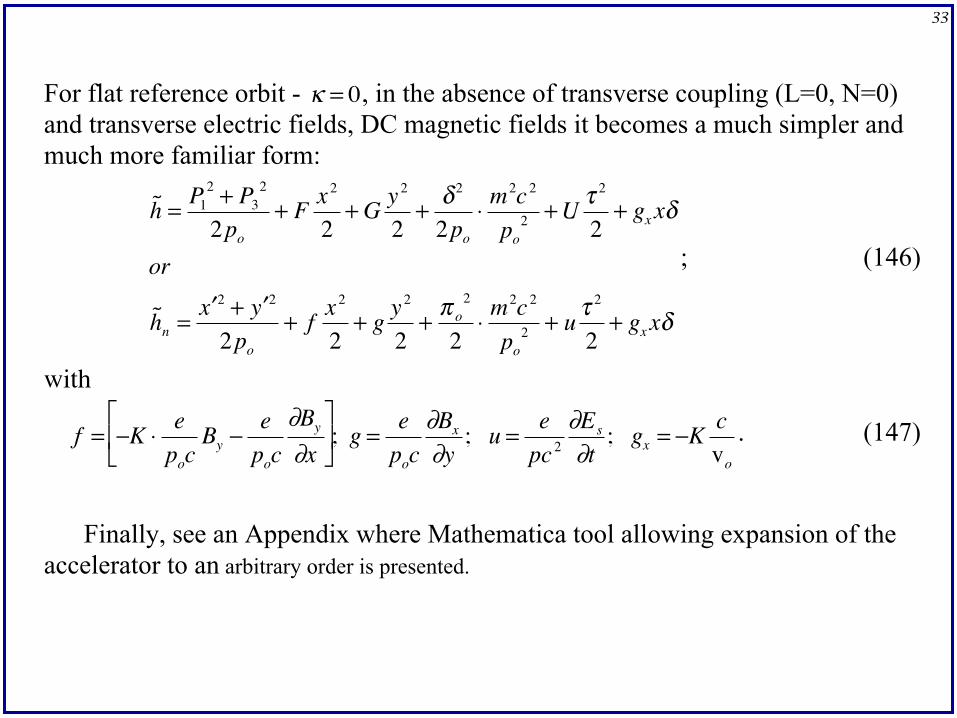
For flat reference orbit -

�

κ = 0, in the absence of transverse coupling (L=0, N=0) and transverse electric fields, DC magnetic fields it becomes a much simpler and much more familiar form:

�

˜ h = P12 + P3

2

2po

+ F x 2

2+ G y 2

2+ δ 2

2po

⋅ m2c 2

po2 + U τ 2

2+ gx xδ

or

˜ h n =′ x 2 + ′ y 2

2po

+ f x 2

2+ g y 2

2+ π o

2

2⋅ m2c 2

po2 + u τ

2

2+ gx xδ

; (146)

with

�

f = −K ⋅ epoc

By −epoc

∂By

∂x⎡

⎣ ⎢

⎤

⎦ ⎥ ; g = e

poc∂Bx

∂y; u = e

pc 2∂Es

∂t; gx = −K c

vo

. (147)

Finally, see an Appendix where Mathematica tool allowing expansion of the

accelerator to an arbitrary order is presented.