Lecture 4 - USPAS | U.S. Particle Accelerator School

Lecture 4:

Synchrotron Radiation

Yunhai Cai SLAC National Accelerator Laboratory

June 13, 2017

USPAS June 2017, Lisle, IL, USA

!"

#"

$"

%

ρ

&"

θ

% '"("

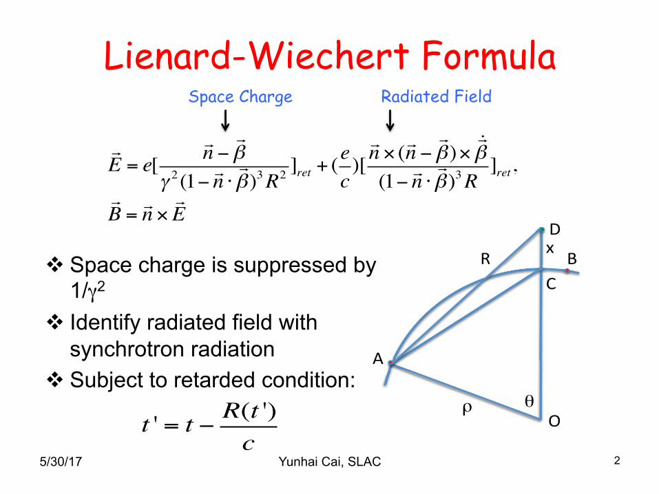
Lienard-Wiechert Formula

!E = e[

!n −!β

γ 2 (1− !n ⋅!β)3R2

]ret + (ec)[!n × (!n −

!β)×!"β

(1− !n ⋅!β)3R

]ret,!B = !n ×

!E

v Space charge is suppressed by 1/γ2

v  Identify radiated field with synchrotron radiation

v Subject to retarded condition:

2

Space Charge Radiated Field

t ' = t − R(t ')c

5/30/17 Yunhai Cai, SLAC

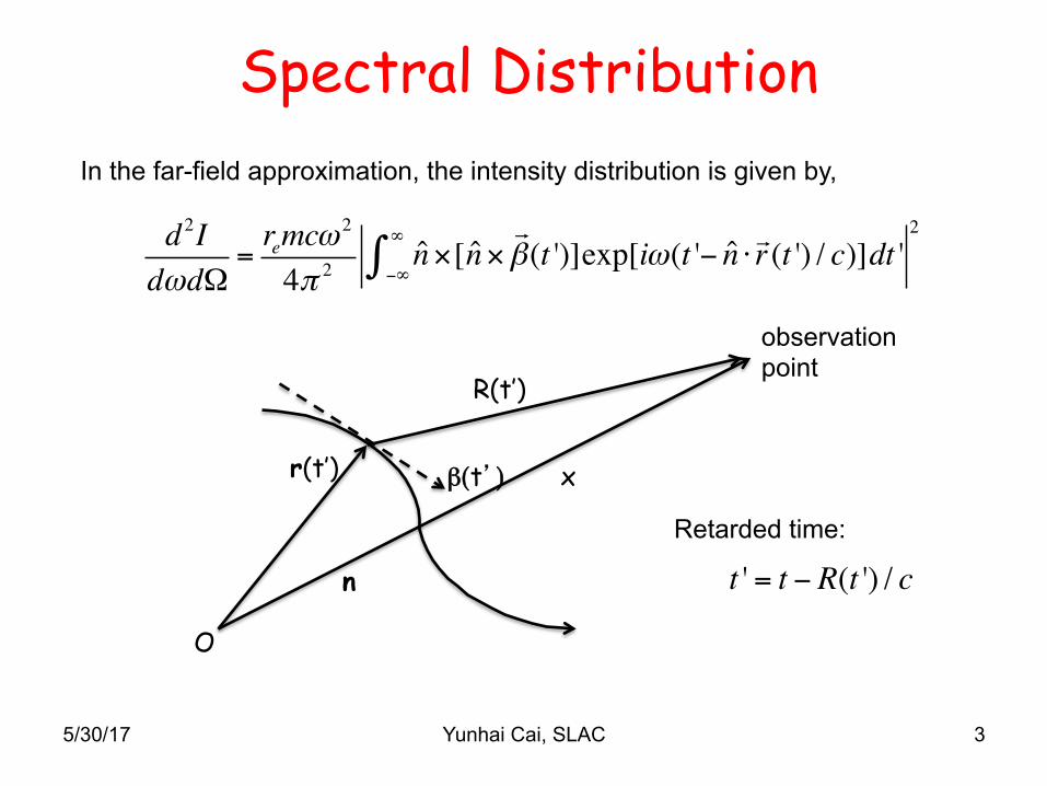
Spectral Distribution

5/30/17 Yunhai Cai, SLAC 3

d 2IdωdΩ

=remcω

2

4π 2 n×[n×!β(t ')]exp[iω(t '− n ⋅ !r (t ') / c)]dt '

−∞

∞

∫2

In the far-field approximation, the intensity distribution is given by,

O

n

β(t’)r(t’) x

observation point

t ' = t − R(t ') / cRetarded time:

R(t’)

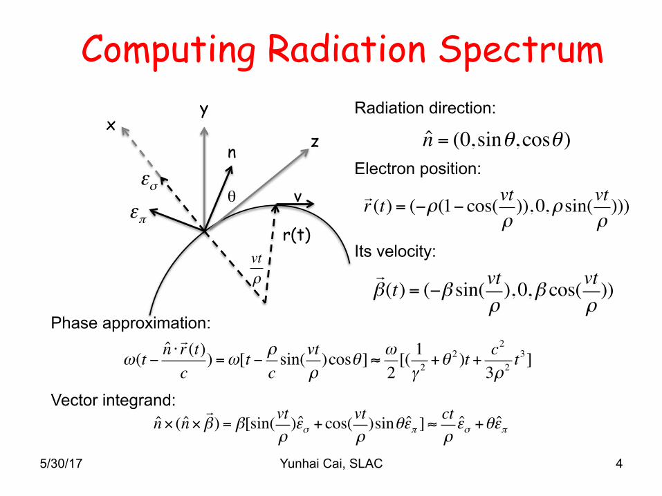
Computing Radiation Spectrum


x y

z

θ

n

v

n = (0,sinθ, cosθ )Radiation direction:

r(t)

Electron position: !r (t) = (−ρ(1− cos(vt

ρ)), 0,ρ sin(vt

ρ)))

Its velocity: !β(t) = (−β sin(vt

ρ), 0,β cos(vt

ρ))

εσεπ

vtρ

ω(t − n ⋅!r (t)c

) =ω[t − ρcsin(vt

ρ)cosθ ] ≈ ω

2[( 1γ 2+θ 2 )t + c2

3ρ2t3]

Phase approximation:

Vector integrand: n× (n×

!β) = β[sin(vt

ρ)εσ + cos(

vtρ)sinθεπ ] ≈

ctρεσ +θεπ

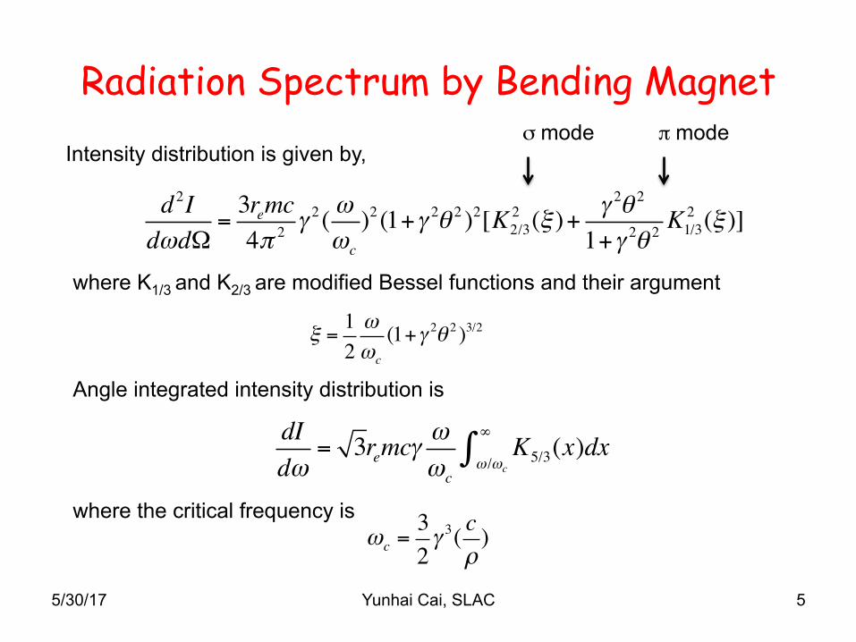
Radiation Spectrum by Bending Magnet


ξ =12ωωc

(1+γ 2θ 2 )3/2

d 2IdωdΩ

=3remc4π 2 γ

2 (ωωc

)2 (1+γ 2θ 2 )2[K2/32 (ξ )+ γ 2θ 2

1+γ 2θ 2K1/32 (ξ )]

Intensity distribution is given by,

where K1/3 and K2/3 are modified Bessel functions and their argument

dIdω

= 3remcγωωc

K5/3ω /ωc

∞

∫ (x)dx

Angle integrated intensity distribution is

ωc =32γ 3( c

ρ)

where the critical frequency is

σ mode π mode

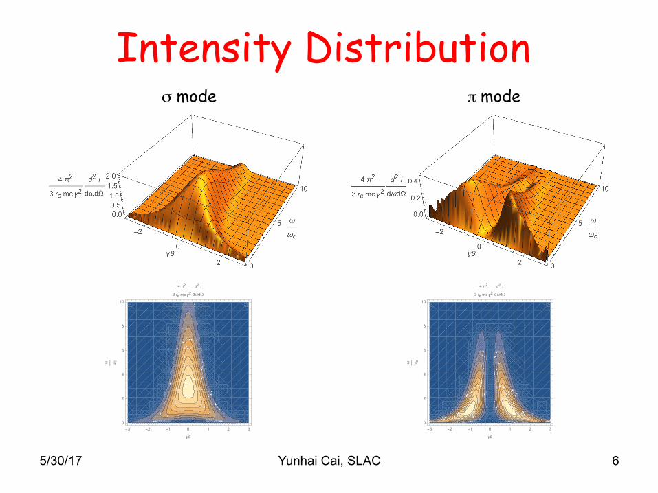
Intensity Distribution

-3 -2 -1 0 1 2 30

2

4

6

8

10

γθ

ω ωc

4 π2

3 re mcγ2d2 I

dωdΩ

-3 -2 -1 0 1 2 30

2

4

6

8

10

γθ

ω ωc

4 π2

3 re mcγ2d2 I

dωdΩ


σ mode π mode

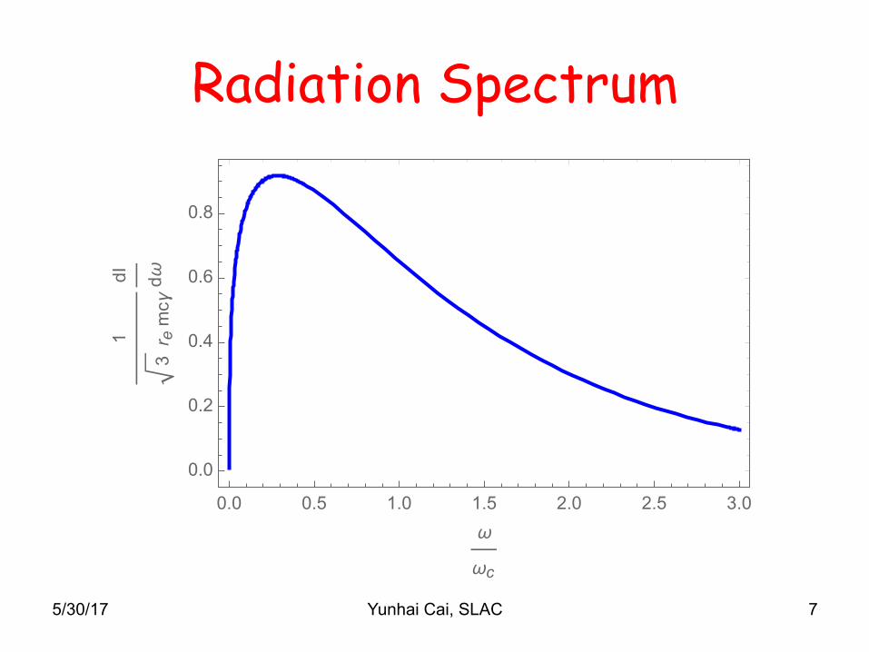
Radiation Spectrum


0.0 0.5 1.0 1.5 2.0 2.5 3.0

0.0

0.2

0.4

0.6

0.8

ω

ωc

1

3r emcγ

dI dω

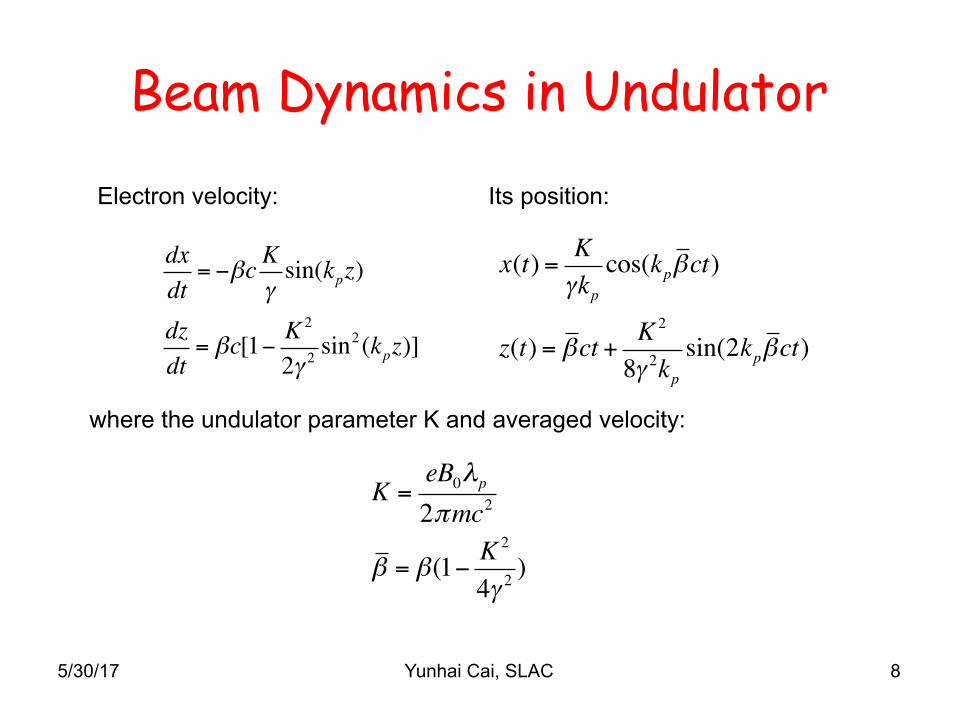
Beam Dynamics in Undulator


dxdt= −βc K

γsin(kpz)

dzdt= βc[1− K

2

2γ 2sin2(kpz)]

Electron velocity:

where the undulator parameter K and averaged velocity:

K =eB0λp

2πmc2

β = β(1− K2

4γ 2)

Its position:

x(t) = Kγkp

cos(kpβct)

z(t) = βct + K 2

8γ 2kpsin(2kpβct)

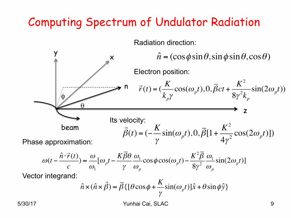
Computing Spectrum of Undulator Radiation


y x

z

φθ

n

beam

n = (cosφ sinθ, sinφ sinθ, cosθ )Radiation direction:

Electron position: !r (t) = ( K

kpγcos(ω pt), 0,βct +

K 2

8γ 2kpsin(2ω pt))

Its velocity: !β(t) = (−K

γsin(ω pt), 0,β[1+

K 2

4γ 2cos(2ω pt)])

ω(t − n ⋅!r (t)c

) ≈ ωω1

[ω pt −Kβθγ

ω1

ω p

cosφ cos(ω pt)−K 2β8γ 2

ω1

ω p

sin(2ω pt)]

Phase approximation:

Vector integrand: n× (n×

!β) ≈ β{[θ cosφ + K

γsin(ω pt)]x +θ sinφ y}

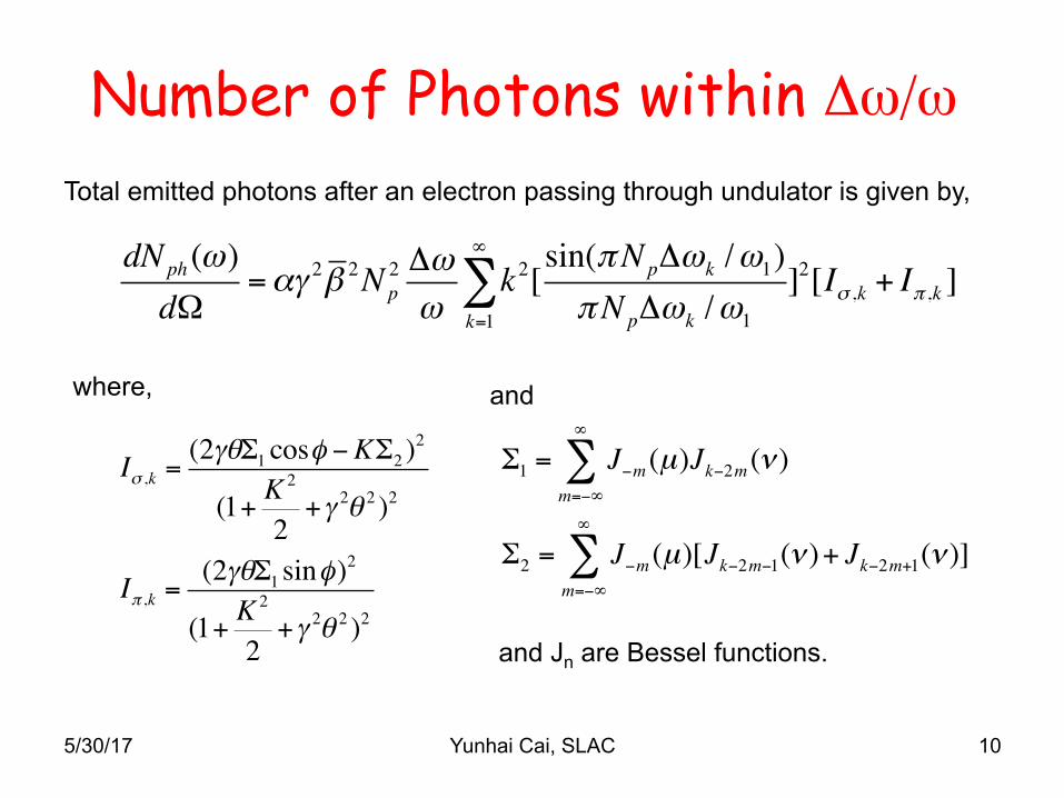
Number of Photons within Δω/ω


dNph (ω)dΩ

=αγ 2β 2Np2 Δωω

k2k=1

∞

∑ [sin(πNpΔωk /ω1)πNpΔωk /ω1

]2[Iσ ,k + Iπ ,k ]

Total emitted photons after an electron passing through undulator is given by,

where,

Iσ ,k =(2γθΣ1 cosφ −KΣ2 )

2

(1+ K2

2+γ 2θ 2 )2

Iπ ,k =(2γθΣ1 sinφ)

2

(1+ K2

2+γ 2θ 2 )2

and

Σ1 = J−m (µ)Jk−2m (ν )m=−∞

∞

∑

Σ2 = J−m (µ)[Jk−2m−1(ν )m=−∞

∞

∑ + Jk−2m+1(ν )]

and Jn are Bessel functions.

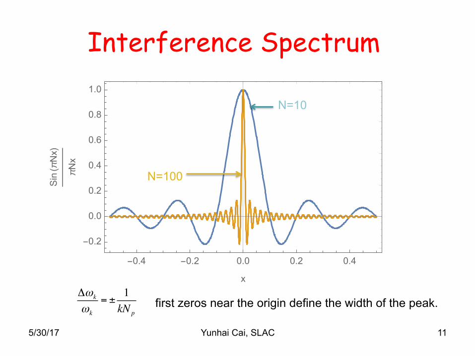
Interference Spectrum

-0.4 -0.2 0.0 0.2 0.4

-0.2

0.0

0.2

0.4

0.6

0.8

1.0

x

Sin(πNx)

πNx


N=10

N=100

Δωk

ωk

= ±1kNp

first zeros near the origin define the width of the peak.

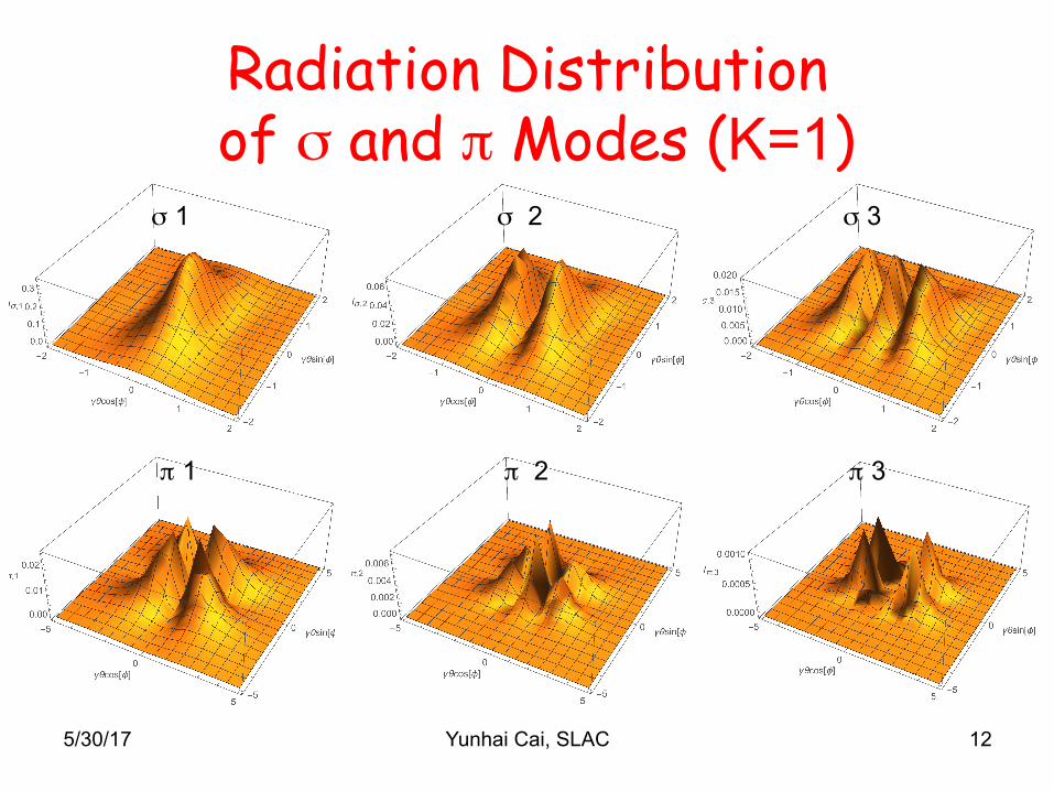
Radiation Distribution of σ and π Modes (K=1)


σ 1 σ 2 σ 3

π 1 π 2 π 3

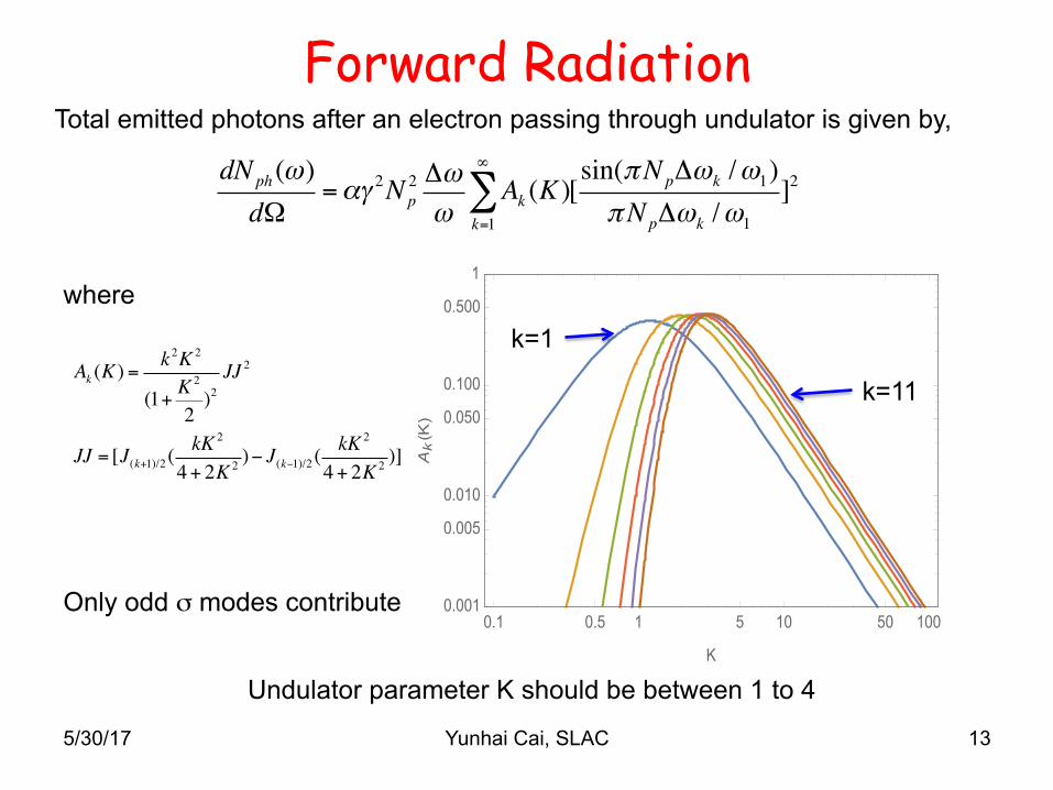
Forward Radiation

0.1 0.5 1 5 10 50 1000.001

0.005

0.010

0.050

0.100

0.500

1

K

Ak(K)


dNph (ω)dΩ

=αγ 2Np2 Δωω

Ak (K )k=1

∞

∑ [sin(πNpΔωk /ω1)πNpΔωk /ω1

]2

Total emitted photons after an electron passing through undulator is given by,

Ak (K ) =k2K 2

(1+ K2

2)2JJ 2

JJ = [J(k+1)/2 (kK 2

4+ 2K 2 )− J(k−1)/2 (kK 2

4+ 2K 2 )]

where

Only odd σ modes contribute

k=1

k=11

Undulator parameter K should be between 1 to 4

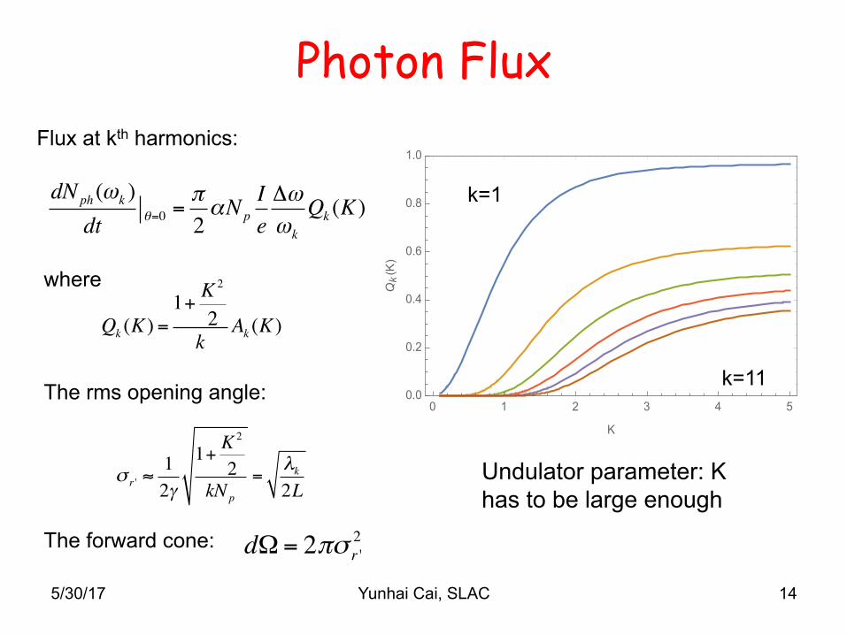
Photon Flux

0 1 2 3 4 50.0

0.2

0.4

0.6

0.8

1.0

K

Qk(K)


dNph (ωk )dt θ=0 =

π2αNp

IeΔωωk

Qk (K )k=1

where

Flux at kth harmonics:

Qk (K ) =1+ K

2

2k

Ak (K )

Undulator parameter: K has to be large enough

k=11 The rms opening angle:

σ r ' ≈12γ

1+ K2

2kNp

=λk2L

The forward cone: dΩ = 2πσ r '2

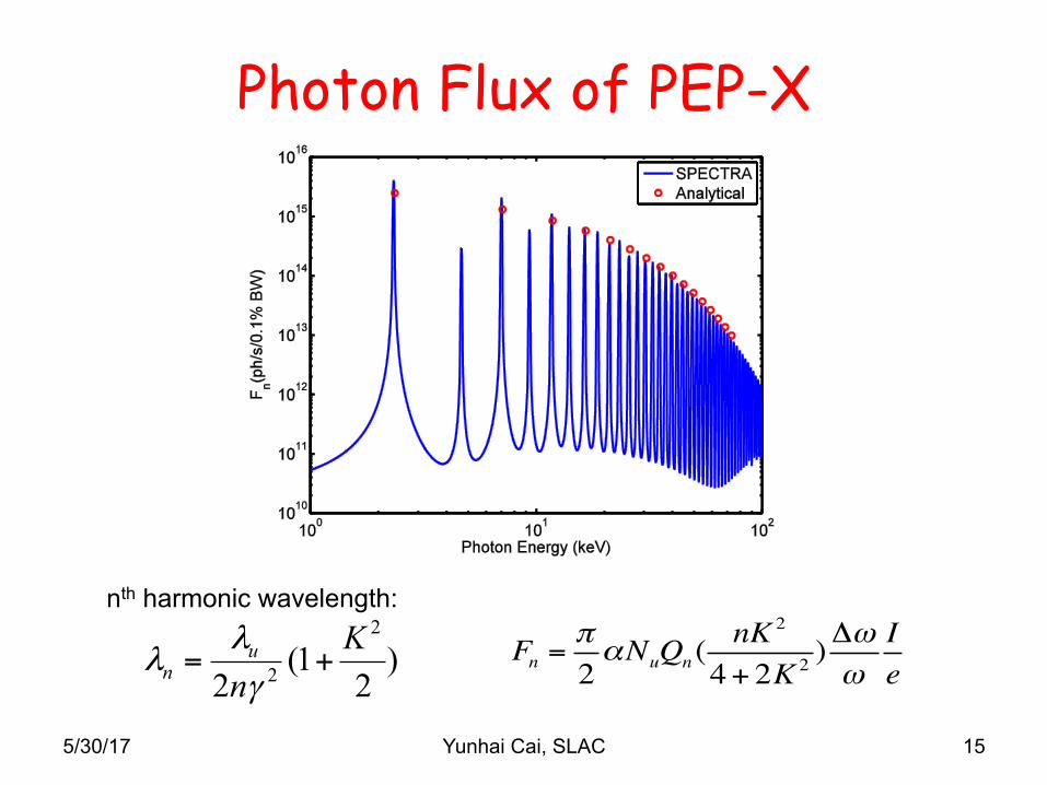
Photon Flux of PEP-X

)2

1(2

2

2

Knu

n +=γλ

λ

nth harmonic wavelength:

Fn =π2αNuQn (

nK 2

4+ 2K 2 )Δωω

Ie


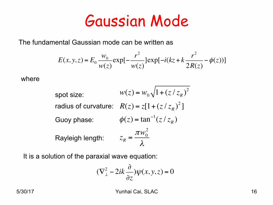
Gaussian Mode


E(x, y, z) = E0w0w(z)

exp[− r2

w(z)]exp[−i(kz+ k r2

2R(z)−φ(z))]

The fundamental Gaussian mode can be written as

w(z) = w0 1+ (z / zR )2

R(z) = z[1+ (z / zR )2 ]

φ(z) = tan−1(z / zR )

zR =πw0

2

λ

where

spot size:

radius of curvature:

Guoy phase:

Rayleigh length:

(∇⊥2 − 2ik ∂

∂z)ψ(x, y, z) = 0

It is a solution of the paraxial wave equation:

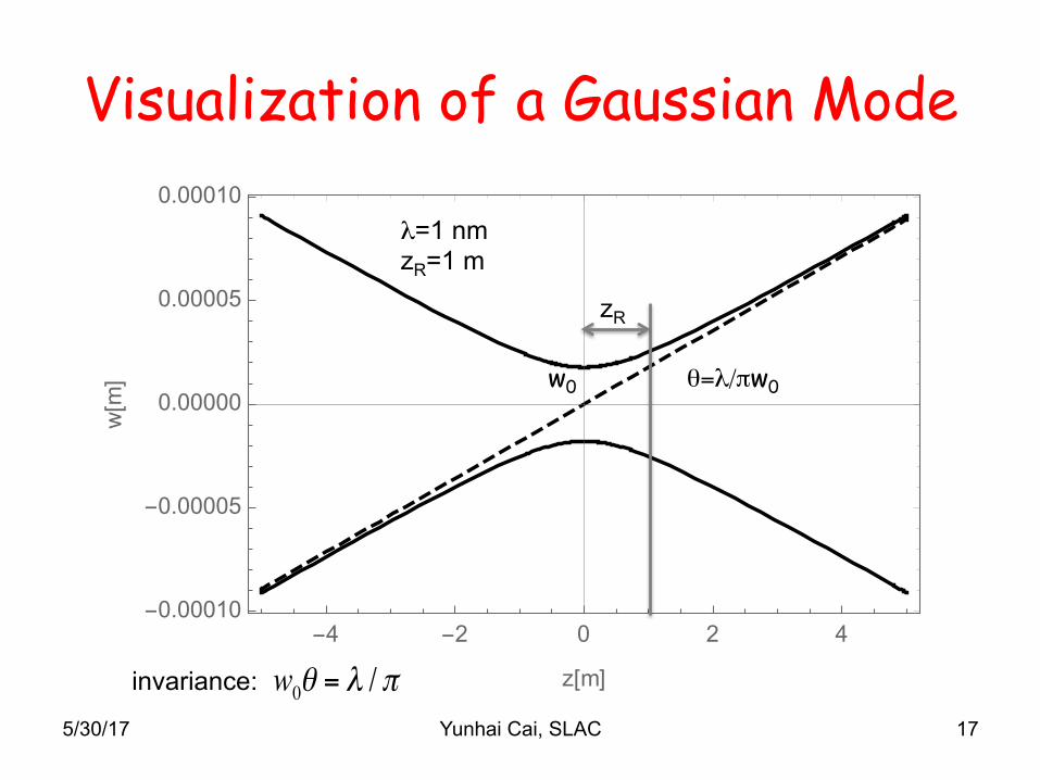
Visualization of a Gaussian Mode

-4 -2 0 2 4-0.00010

-0.00005

0.00000

0.00005

0.00010

z[m]

w[m

]


θ=λ/πw0 w0

zR

λ=1 nm zR=1 m

w0θ = λ /πinvariance:

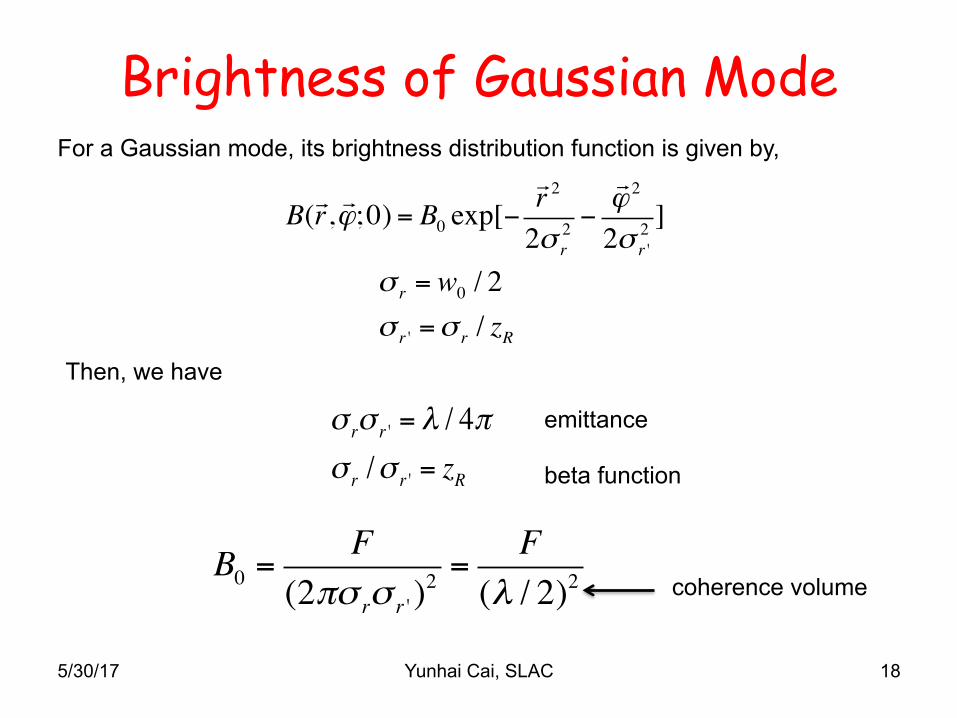
Brightness of Gaussian Mode


σ r = w0 / 2σ r ' =σ r / zR

For a Gaussian mode, its brightness distribution function is given by,

Then, we have

B0 =F

(2πσ rσ r ' )2 =

F(λ / 2)2

B(!r, !ϕ;0) = B0 exp[−!r 2

2σ r2 −!ϕ 2

2σ r '2 ]

σ rσ r ' = λ / 4πσ r /σ r ' = zR

emittance

beta function

coherence volume

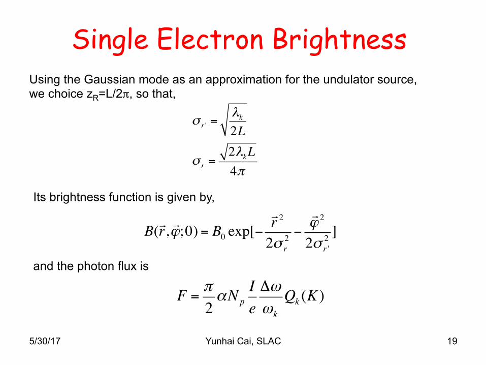
Single Electron Brightness


σ r ' =λk2L

σ r =2λkL4π

Using the Gaussian mode as an approximation for the undulator source, we choice zR=L/2π, so that,

F = π2αNp

IeΔωωk

Qk (K )

and the photon flux is

B(!r, !ϕ;0) = B0 exp[−!r 2

2σ r2 −!ϕ 2

2σ r '2 ]

Its brightness function is given by,

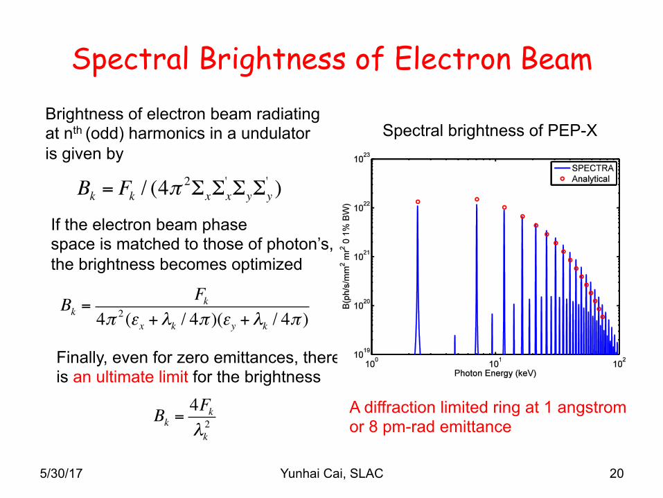
Spectral Brightness of Electron Beam Brightness of electron beam radiating at nth (odd) harmonics in a undulator is given by

Bk = Fk / (4π2ΣxΣx

' ΣyΣy' )

Bk =Fk

4π 2 (εx +λk / 4π )(εy +λk / 4π )

If the electron beam phase space is matched to those of photon’s, the brightness becomes optimized

Finally, even for zero emittances, there is an ultimate limit for the brightness

Bk =4Fkλk2

Spectral brightness of PEP-X

A diffraction limited ring at 1 angstrom or 8 pm-rad emittance

20 Yunhai Cai, SLAC 5/30/17

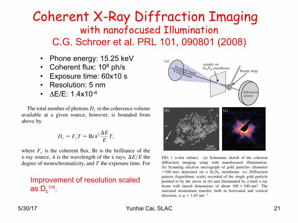
Coherent X-Ray Diffraction Imaging with nanofocused Illumination

C.G. Schroer et al. PRL 101, 090801 (2008)

Coherent X-Ray Diffraction Imaging with Nanofocused Illumination

C.G. Schroer,1 P. Boye,1 J.M. Feldkamp,1 J. Patommel,1 A. Schropp,1,3 A. Schwab,1 S. Stephan,1 M. Burghammer,2

S. Schoder,2 and C. Riekel2

1Institute of Structural Physics, Technische Universitat Dresden, D-01062 Dresden, Germany2ESRF, B. P. 220, F-38043 Grenoble, France

3HASYLAB at DESY, Notkestr. 85, D-22607 Hamburg, Germany(Received 26 April 2008; published 29 August 2008)

Coherent x-ray diffraction imaging is an x-ray microscopy technique with the potential of reaching

spatial resolutions well beyond the diffraction limits of x-ray microscopes based on optics. However, the

available coherent dose at modern x-ray sources is limited, setting practical bounds on the spatial

resolution of the technique. By focusing the available coherent flux onto the sample, the spatial resolution

can be improved for radiation-hard specimens. A small gold particle (size<100 nm) was illuminated with

a hard x-ray nanobeam (E ¼ 15:25 keV, beam dimensions " 100# 100 nm2) and is reconstructed from

its coherent diffraction pattern. A resolution of about 5 nm is achieved in 600 s exposure time.

DOI: 10.1103/PhysRevLett.101.090801 PACS numbers: 07.85.Tt, 42.30.Rx, 78.70.Ck

Determining the structure of nanoscale objects, such as,for example, biomolecules in their cellular environment,small particles for industrial catalysis, and nanoelectronicdevices, is crucial to understand their function and to pushstructural biology, chemistry, and nanotechnology to newfrontiers. X-ray microscopy is well suited to investigatesuch systems [1], as it allows one to image them with highspatial resolution, with minimal sample preparation (e.g.,shock-freezing), and inside environments for in situ stud-ies, e.g., catalytic reactors or high magnetic fields. Cur-rently, all direct x-ray microscopy techniques are limited inspatial resolution to a few 10 nm, due to aberrations and thelimited numerical aperture of today’s x-ray optics [2].Coherent x-ray diffraction imaging (CXDI) does not relyon x-ray optics and, therefore, has the potential to push thespatial resolution limit to well beyond that of direct imag-ing techniques. In addition, x-ray free-electron lasers(XFELs) will provide ultra short and highly brilliantx-ray pulses, potentially making time resolved CXDI stud-ies of molecular dynamics possible [3–7].

In CXDI, the object is illuminated with coherent x raysand its far-field diffraction pattern is recorded without anyoptic [3,8–10]. From this diffraction pattern, the wave fieldbehind the object is reconstructed by iteratively solving thephase problem [8,11–14]. Three-dimensional imaging ispossible by recording a (tomographic) series of diffractionpatterns [9,15–18]. Coherent illumination of the object iscrucial to this technique, and the coherent dose on thesample determines the spatial resolution. As the coherentflux at modern synchrotron radiation sources is limited,CXDI experiments require long exposure times, and thespatial resolutions obtained so far have been similar tothose of direct imaging techniques, lying in the range ofa few 10 nm.

In this Letter, we report on a CXDI experiment withnanofocused illumination, from which the small gold par-

ticle under investigation was reconstructed with 5 nmspatial resolution. As a result of the nanofocusing, thecoherent flux on the sample was efficiently increased,reducing considerably the exposure time at high spatialresolution. This opens the way to combine scanning mi-croscopy and CXDI to obtain a spatial resolution wellbeyond that of each technique taken by itself [19–22] and

1µm

(b) (c)

focused hardx-ray beambeam stop

sample onSi3N4 membrane

(a)

diffractioncamera

FIG. 1 (color online). (a) Schematic sketch of the coherentdiffraction imaging setup with nanofocused illumination.(b) Scanning electron micrograph of gold particles (diameter"100 nm) deposited on a Si3N4 membrane. (c) Diffractionpattern (logarithmic scale) recorded of the single gold particlepointed to by the arrow in (b) and illuminated by a hard x-raybeam with lateral dimensions of about 100# 100 nm2. Themaximal momentum transfer, both in horizontal and verticaldirection, is q ¼ 1:65 nm$1.

PRL 101, 090801 (2008) P HY S I CA L R EV I EW LE T T E R Sweek ending

29 AUGUST 2008

0031-9007=08=101(9)=090801(4) 090801-1 ! 2008 The American Physical Society5/30/17 Yunhai Cai, SLAC 21

is crucial to single particle diffraction experiments at futurefree-electron laser sources [4].

The nano-CXDI experiment was realized with our hardx-ray microscope set up at beam line ID13 of the EuropeanSynchrotron Radiation Facility (ESRF). A schematicsketch of the experimental setup is shown in Fig. 1(a):The sample is fully illuminated by a diffraction limited,nanofocused hard x-ray beam. The directly transmittedbeam is blocked by a beam stop, and the diffraction patternof the object is recorded in forward scattering geometry ona diffraction camera [cf. Fig. 1(a)]. This diffraction patternis then used to reconstruct the projected electron density ofthe object by iterative schemes.

The x rays from an in-vacuum undulator source weremonochromatized with a channel-cut Si (111) monochro-

mator at an energy of E ¼ 15:25 keV (wavelength ! ¼0:813 !A). Two crossed refractive nanofocusing lenses(NFLs) [23,24] were used in the scanning microscopethat was set up at a distance of L1 ¼ 44 m from the source.In the focus, a beam size slightly larger than 100"100 nm2 was measured using a knife-edge technique.The flux in this beam exceeded 108 ph=s yielding a gainin intensity of g ¼ 104.

The sample, a single gold nanoparticle supported by aSi3N4 membrane, was placed in the nanofocus. Figure 1(b)shows a cluster of such particles on a Si3N4 membrane of50 nm thickness. The white arrow in Fig. 1(b) points to thegold particle investigated here. It was located by fluores-cence mapping. In this first proof-of-principle nano-CXDIexperiment, we chose a gold particle because of its com-parably large scattering cross section and its relative radia-tion hardness.

A diffraction pattern of the sample was recorded with 10one-minute exposures on a diffraction camera (FReLoN4M, 50 "m pixel size) located at a distance of 1250 mmbehind the sample. As the beam stop was too large to coverthe central diffraction maximum, alone, it was moved upand down to record the inner parts of the diffraction patternin several steps. In Fig. 1(c), the combined diffractionpattern is shown. It is oversampled by about a factor of20 in both directions and has inversion symmetry exceptfor a reduction in intensity in the upper right quadrant dueto the support of the beam stop.

The diffraction pattern in Fig. 1(c) was used to recon-struct the gold particle using the hybrid input-output (HIO)method [11,25] together with the so-called shrink-wrapalgorithm [26]. We performed 200 independent reconstruc-tions out of which 191 converged to similar enantiomorphs[27] of the gold particle [cf. Fig. 2(a)]. These were com-bined to an average reconstruction shown in Fig. 2(b).From the root mean square variation of the reconstructions,the relative error of the electron density can be estimated.A horizontal section through the center of the particle isshown in Fig. 2(c). The reconstruction error is nearlyconstant over the whole object, and its border has a fuzzi-ness of one to two pixels, corresponding to a spatial

resolution of 3.8 to 7.6 nm, respectively. Evaluating thephase retrieval transfer function [9,10] by determining thehighest momentum transfer for which the phase correlationin the reconstruction is above 10%, a corresponding halfperiod of 4.3 nm is obtained, in agreement with the realspace estimate for the spatial resolution given above.The spatial resolution of CXDI is effectively limited by

the strong decay of the diffraction intensity with increasingscattering vector ~q. For a generic object, the diffractionintensity decays with a power law q## (# $ 4) [28]. Thus,an increase in resolution by 1 order of magnitude for agiven experimental setup requires an increase in dose byabout 4 orders of magnitude.The total number of photonsDc in the coherence volume

available at a given source, however, is bounded fromabove by

Dc ¼ FcT ¼ Br!2 "E

ET;

where Fc is the coherent flux, Br is the brilliance of thex-ray source, ! is the wavelength of the x rays, "E=E thedegree of monochromaticity, and T the exposure time. Forstorage ring based x-ray sources, the brilliance Br can notbe significantly increased much further. In addition, toapproach nanometer resolution and below, the require-ments on the wavelength ! and the monochromaticity"E=E become more and more stringent, reducing themaximal coherent flux. One way to increase the dose onthe sample and thus the spatial resolution is to increase theexposure time T. This scheme has been followed in mosthigh resolution experiments, so far. However, the gain in

FIG. 2. (a) Two individual reconstructions of the gold particleusing the HIO algorithm, a left- and a right-handed one. Toobtain the average particle shape from a series of reconstructionswith random initial phases, the right-handed reconstructionswere inverted and averaged together with the left-handed ones.(b) Reconstructed projected electron density of the gold nano-particle shown in Fig. 1(b) after averaging the series of recon-structions. (c) Horizontal section through the center of theparticle shown in (b). The error bars indicate rms variations inthe density for the series of independent reconstructions.

PRL 101, 090801 (2008) P HY S I CA L R EV I EW LE T T E R Sweek ending

29 AUGUST 2008

090801-2

•  Phone energy: 15.25 keV •  Coherent flux: 108 ph/s •  Exposure time: 60x10 s •  Resolution: 5 nm •  ΔE/E: 1.4x10-4

Improvement of resolution scaled as Dc

1/4.

ESRF Lecture Series on Coherent X-rays and their Applications, Lecture 1, Malcolm Howells

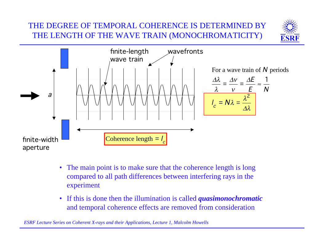
THE DEGREE OF TEMPORAL COHERENCE IS DETERMINED BYTHE LENGTH OF THE WAVE TRAIN (MONOCHROMATICITY)

For a wave train of N periods!"

"=!#

#=!E

E$

1

N

lc

= N" ="

2

!"

wavefronts

a

finite-widthaperture

finite-lengthwave train

Coherence length = l

c

• The main point is to make sure that the coherence length is longcompared to all path differences between interfering rays in theexperiment

• If this is done then the illumination is called quasimonochromaticand temporal coherence effects are removed from consideration


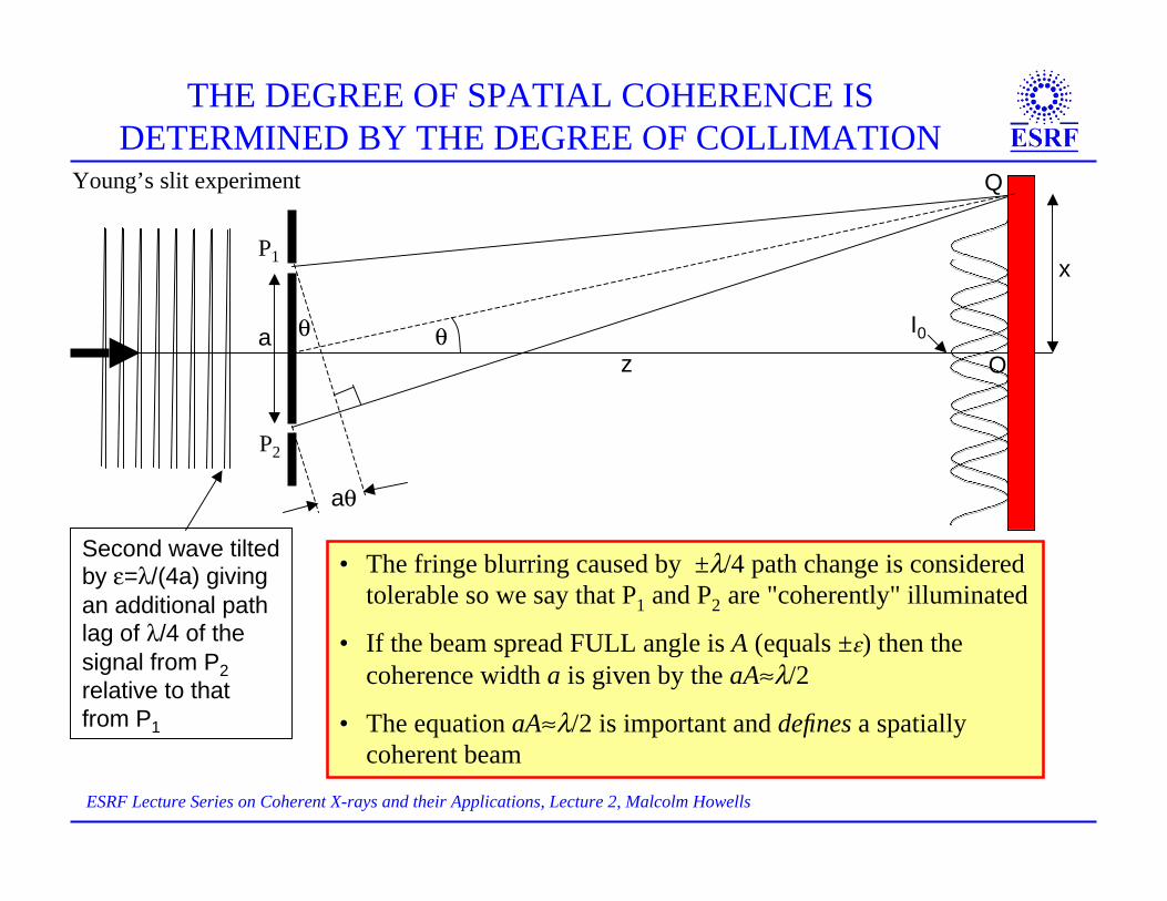
THE DEGREE OF SPATIAL COHERENCE ISDETERMINED BY THE DEGREE OF COLLIMATION

P2

P1

az

θθ

aθ

x

O

Q

Second wave tiltedby ε=λ/(4a) givingan additional pathlag of λ/4 of thesignal from P2relative to thatfrom P1

I0

• The fringe blurring caused by ±λ/4 path change is consideredtolerable so we say that P1 and P2 are "coherently" illuminated

• If the beam spread FULL angle is A (equals ±ε) then thecoherence width a is given by the aA≈λ/2

• The equation aA≈λ/2 is important and defines a spatiallycoherent beam

Young’s slit experiment


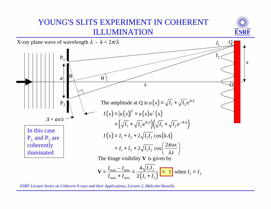
YOUNG'S SLITS EXPERIMENT IN COHERENTILLUMINATION

P2

P1

az

θθ

Δ = ax/z

x

O

Q

I x( ) = u x( )2

= u x( )u! x( )

= I1 + I2 eik"( ) I1 + I2 e#ik"

( )

X-ray plane wave of wavelength λ - k = 2π/λ

I2

I1

The fringe visibility V is given by

V =Imax ! Imin

Imax + Imin=

4 I1I2

2 I1 + I2( )= 1 when I1 = I2

The amplitude at Q is u x( ) = I1 + I2 eik!

In this caseP1 and P2 arecoherentlyiluminated

I x( ) = I1 + I2 + 2 I1I2 cos k!( )

= I1 + I2 + 2 I1I2 cos 2"ax#z

$%&

'()


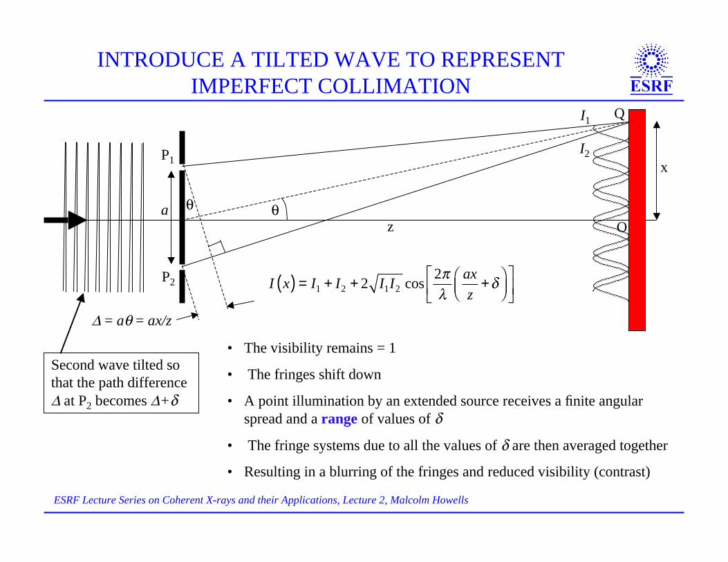
INTRODUCE A TILTED WAVE TO REPRESENTIMPERFECT COLLIMATION

P2

P1

az

θθ

Δ = aθ = ax/z

x

O

Q

I2

I1

Second wave tilted sothat the path differenceΔ at P2 becomes Δ+δ

I x( ) = I1 + I2 + 2 I1I2 cos 2!"

axz

+#$%&

'()

*

+,-

./

• The visibility remains = 1

• The fringes shift down

• A point illumination by an extended source receives a finite angularspread and a range of values of δ

• The fringe systems due to all the values of δ are then averaged together

• Resulting in a blurring of the fringes and reduced visibility (contrast)


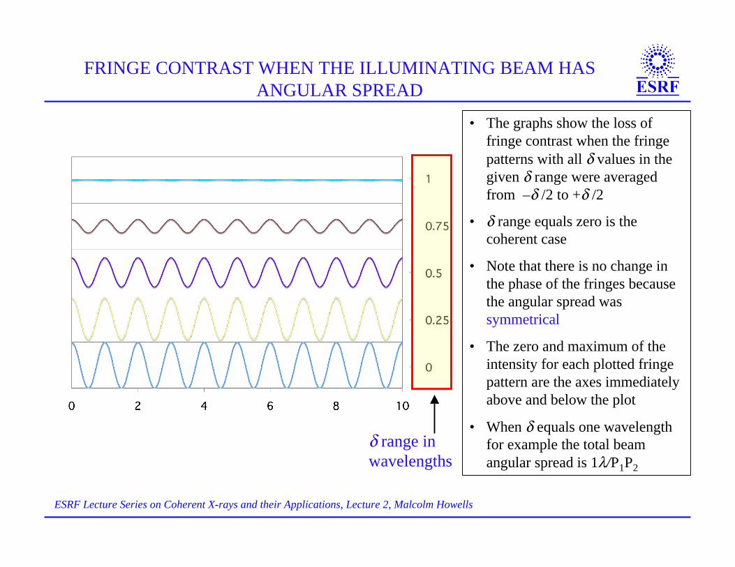
• The graphs show the loss offringe contrast when the fringepatterns with all δ values in thegiven δ range were averagedfrom –δ /2 to +δ /2

• δ range equals zero is thecoherent case

• Note that there is no change inthe phase of the fringes becausethe angular spread wassymmetrical

• The zero and maximum of theintensity for each plotted fringepattern are the axes immediatelyabove and below the plot

• When δ equals one wavelengthfor example the total beamangular spread is 1λ/P1P2

FRINGE CONTRAST WHEN THE ILLUMINATING BEAM HASANGULAR SPREAD

δ range inwavelengths

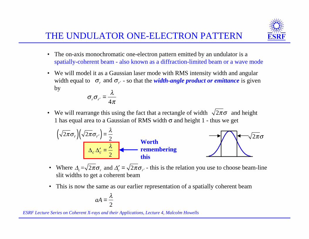
• The on-axis monochromatic one-electron pattern emitted by an undulator is aspatially-coherent beam - also known as a diffraction-limited beam or a wave mode

• We will model it as a Gaussian laser mode with RMS intensity width and angularwidth equal to - so that the width-angle product or emittance is givenby


THE UNDULATOR ONE-ELECTRON PATTERN

• We will rearrange this using the fact that a rectangle of width and height1 has equal area to a Gaussian of RMS width σ and height 1 - thus we get

! r and !"r

! r! "r =#

4$

2!"

2!" r( ) 2!" #r( ) =$

2

%c #%c =$

2

• Where - this is the relation you use to choose beam-lineslit widths to get a coherent beam

• This is now the same as our earlier representation of a spatially coherent beam

!c = 2"# r and $!c = 2"#$r

aA =!

2

Worthrememberingthis

2!"

References

1)  J.D. Jackson, Classical Electrodynamics, Third Edition, John Wiley & Son, Inc. 1999

2)  H. Wiedemann, Synchrotron Radiation, Springer-Verlag Berlin Heidelberg 2003

3)  Kwang-Je Kim, “Characteristics of Synchrotron Radiation,” AIP Proc. No. 184 (AIP, New York, 1989), pp. 565–632

4)  Malcolm Howells, ESRF lecture series of coherent X-ray and their applications

5/30/17 Yunhai Cai SLAC 22

Lecture 4 - USPAS | U.S. Particle Accelerator School

Documents

Transcript of Lecture 4 - USPAS | U.S. Particle Accelerator School