OSKAR TILL - Chalmers Publication Library (CPL):...

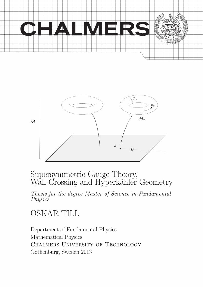
B

M

a

Ma

θe

θm

Supersymmetric Gauge Theory,Wall-Crossing and Hyperkahler Geometry

Thesis for the degree Master of Science in FundamentalPhysics

OSKAR TILL

Department of Fundamental Physics

Mathematical Physics

Chalmers University of Technology

Gothenburg, Sweden 2013

Abstract

In this thesis we study moduli spaces of four-dimensional N = 2 supersymmetricgauge theories. We focus on the vector multiplet moduli space and describe howthe rigid special geometry of the Coulomb branch determines the couplings in theeffective Lagrangian. Compactification to three dimensions gives rise to an N = 4theory whose moduli space is hyperkahler. The twistor space construction of thishyperkahler metric is presented and put in the context of Gaiotto, Moore andNeitzke’s physical interpretation of the solution by Kontsevich and Soibelman ofthe wall-crossing problem.

Acknowledgements

I want to thank my supervisor Daniel Persson for all help and valuable discussionswhile introducing me to the subjects of this thesis. I’m also grateful to all thefaculty members and students of the Department of Fundamental Physics for agood and friendly environment during my thesis work. I especially mention BengtE W Nilsson for good advise and taking time for any questions. Thank you HenrikGustafsson for proof-reading and giving comments before presentation of my work.Last and not the least, thank you Denis Karateev, Fredrik Strannerdahl, JoakimEdlund and Tobias Wenger for the help, the discussions and the nice company.

Oskar Till, Goteborg 2013-01-17

CONTENTS

Contents

1 Introduction 2

2 N = 2 Gauge Theories in Four Dimensions 3

2.1 The Field Theory . . . . . . . . . . . . . . . . . . . . . . . . . . . . 4

2.2 The Moduli Space . . . . . . . . . . . . . . . . . . . . . . . . . . . . 5

2.2.1 The Coulomb Branch and Supersymmetric Constraints . . . 6

2.3 Electric and Magnetic Charges . . . . . . . . . . . . . . . . . . . . . 10

2.4 Rigid Special Kahler Geometry . . . . . . . . . . . . . . . . . . . . 11

2.5 The Central Charge . . . . . . . . . . . . . . . . . . . . . . . . . . . 13

3 BPS-states 14

3.1 The Supersymmetry Algebra . . . . . . . . . . . . . . . . . . . . . . 14

3.2 Representations . . . . . . . . . . . . . . . . . . . . . . . . . . . . . 15

3.2.1 Long Representations . . . . . . . . . . . . . . . . . . . . . . 18

3.2.2 BPS Representations . . . . . . . . . . . . . . . . . . . . . . 19

4 Wall-Crossing 20

4.1 The BPS Index . . . . . . . . . . . . . . . . . . . . . . . . . . . . . 21

4.2 The Wall-Crossing Formula . . . . . . . . . . . . . . . . . . . . . . 22

5 Compactification to Three Dimensions 27

5.1 The Bosonic Field Content . . . . . . . . . . . . . . . . . . . . . . . 27

5.2 Dimensional Reduction of the Supercharges . . . . . . . . . . . . . 29

1

CONTENTS

5.3 Describing the Hyperkahler Geometry . . . . . . . . . . . . . . . . . 31

5.3.1 The Semiflat Metric . . . . . . . . . . . . . . . . . . . . . . 31

5.3.2 The Ooguri-Vafa Metric . . . . . . . . . . . . . . . . . . . . 33

5.3.3 Twistor Space Description . . . . . . . . . . . . . . . . . . . 36

6 Wall-Crossing in Twistor Space 41

Appendices 46

A Hyperkahler Geometry 46

A.1 Foundations . . . . . . . . . . . . . . . . . . . . . . . . . . . . . . . 46

A.2 Twistor Space Construction of a Hyperkahler Metric . . . . . . . . 48

B Special Geometry and Riemann Surfaces 49

2

1 INTRODUCTION

1 Introduction

The study of supersymmetric gauge theories has been intimately related to com-plex geometry since the birth of the first models in the seventies. There are amultitude of complex manifolds parametrised by the scalar fields. Together the di-mensionality, the amount of supersymmetry and the gauge symmetry restricts thescalar geometries. The possibilities ranges from Riemannian manifolds to highlyrestricted complex manifolds with very specific geometric structures. Starting froma theory in high space-time dimension many of these may be obtained by com-pactification on compact spaces preserving different amounts of supersymmetry.

In this thesis we present the Kahler geometry of the vector multiplet moduli spaceof an N = 2 gauge theory in four dimensions. At generic points of this spacethe gauge group is broken to a maximal Abelian symmetry making the modulispace a rigid special Kahler manifold. When compactifying to three dimensionsan effective N = 4 theory is obtained whose moduli space is hyperkahler.

The representation theory of the N = 2 superalgebra contains representationswhich in a precise sense are ’smaller’ than a generic representation. These arecalled BPS representations or short representations. In general the spectrum of thetheory changes over the moduli space but the BPS spectrum is generically stable.However, at certain loci splitting or fusion of BPS states may occur, dividing themoduli space into subregions of constant spectrum. There is an index, the secondhelicity supertrace, that count (with signs) BPS state degeneracies and hence it islocally constant. The wall-crossing problem is about relating this index betweendifferent regions of the moduli space, defining a global invariant.

The solution of the wall-crossing problem by Kontsevich and Soibelman (KS) in[18] was physically interpreted by Gaiotto, Moore and Neitzke in [13]. They makeuse of the twistor space description of a hyperkahler manifold in terms of Darbouxcoordinates. The main idea of their paper is that the metric is only continuousglobally if the BPS-index satisifies the KS wall-crossing formula.

The BPS states in four dimensions may wrap the compactified direction and in thecompactification limit these field excitations occur as instantons in three dimen-sions. The tower of wrapped states contributes to the moduli space metric and theinstanton corrected geometry may be explicitly constructed in terms of Darbouxcoordinate functions over the twistor space. It is in terms of these functions thewall-crossing problem was adressed.

This thesis is organised as follows. In section 2 the N = 2 field theory in four

3

2 N = 2 GAUGE THEORIES IN FOUR DIMENSIONS

dimensions is introduced, aiming at the scalar geometry. Moduli spaces are thenintroduced in general terms and the constraints from supersymmetry and gaugesymmetry are analysed. The implication of magnetic-electric duality on the geom-etry is presented, leading to the definition of rigid special geometry.

Section 3 is concerned with the representation theory of the N = 2 superalgebra.The BPS bound is derived and the form of the general BPS representations areobtained. We aim the presentation towards the hypermultiplet and the vectormultiplet since they contain the scalars that constitute the moduli space.

In section 4 the BPS index is introduced to separate the BPS representations fromthe non-BPS ones. We analyse under which conditions the spectrum may jumpgiving discontinuities to the BPS-index. Here the KS solution is introduced andthe wall-crossing formula is presented and its interpretation with respect to theBPS spectrum is discussed.

Compactification to three dimensions are performed in section 5. We derive explic-itly how the bosonic field content changes and how the hyperkahler moduli spaceis described as a torus fibration over the Coulomb branch. We introduce and verifythe Darboux coordinate ansatz for the metric in the semi-flat case, when no instan-ton contributions are present. Then the instanton corrected metric is constructedin the case when only electric charges are present. This is the Ooguri-Vafa metric.Finally we describe how the general wall-crossing problem is formulated and howthe KS formula in the BPS-index is necessary for the continuity of the modulispace metric.

In appendix A some background on hyperkahler manifolds and their twistor spacesare presented. Appendix B contains a brief discussion on rigid special Kahlermanifolds in the context of Riemann surface moduli spaces.

2 N = 2 Gauge Theories in Four Dimensions

In this section we review some features of global N = 2 supersymmetric gaugetheories in d = 4. The discussion is inclined towards the scalar field geometryand how it is encoded in the Lagrangian. We restrict to color gauge symmetriesand omit any possible flavour symmetry. The field theory has a large parameterspace of vacua and we see how gauge invariance and supersymmetry puts restric-tions on what theories may be constructed. We will see that these two conceptsbecome closely intertwined and result in a fascinating piece of geometry. The mod-

4


uli space metric determines all couplings in the effective Lagrangian and may beexpressed solely by the prepotential, a holomorphic function of the scalar fields.In [23] Seiberg and Witten solved the SU(2) N = 2 gauge theory by giving theprepotential explicitly.

2.1 The Field Theory

In this section we discuss the bosonic degrees of freedom of the theory and some ofits implications. The notation we set here will come back throughout the followingchapters and some of the objects which are briefly introduced here will be clarifiedlater on. The treatment in this section and the following is close to the one in [3].

The theory we are interested in is the low energy limit of a theory with gaugegroup G. The bosonic fields are complex scalar fields ai, i = 1, . . . , r and gaugefields AI , all in the adjoint representation. We assume that all scalars have a non-zero vacuum expectation value, breaking the rank r gauge group to U(1)r at lowenergies. The general form of the bosonic Lagrangian in two derivatives is

L = −1

2gij(a)Dai ∧ ∗Daj − 1

8π=[τIJ(a)F I ∧ ∗FJ

]+ V (a) (2.1)

where V (a) is some gauge invariant real potential in the scalar fields. g is areal, symmetric and positive definite tensor field. Under an infinitesimal U(1)transformation of the scalars ai → ai + ξiI(a) we introduce Dµ as the covariantderivative with respect to the U(1) gauge field 1-forms AI = AIµdxµ. The covariantexterior derivative acts on the scalars as

Dai = dai + AIξiI (2.2)

treating the generators of the gauge transformation as Killing vectors of isometriesof the parameter space. The field strength F = dA build up a generalised complexfield strength

F I = F I − i ∗ F I (2.3)

where ∗ is the Hodge operator in the Minkowski metric on R1,3. The matrix τ isa complex symmetric function of the scalars which is conventionally splitted as

τIJ =θIJ2π

+ i4π

(e2)IJ(2.4)

5


and if we write out the gauge field part of (2.1) we have

LU(1)r = − 1

(e2)IJF I ∧ ∗F J +

θIJ8π2

F I ∧ F J (2.5)

=1

4π

[−= τIJF I ∧ ∗F J + < τIJF I ∧ F J

],

motivating the generalised field strength (2.3). The kinetic term coefficient func-tion = τ(a) must be positive definite for unitarity and we may identify (e2)IJ(a)as the electromagnetic couplings and θIJ(a) as the theta angles of the topologicalterm F ∧ F . For the path integral to be well defined this angle has to be peri-odic since a topological term can only contribute an integer multiple of 2π to theaction. Physically the θ-term counts the instanton number of the quantised fieldconfiguration which is an integer, giving the θ-angles the periodicity θ = θ + 2π.This is equivalent to

τ = τ + 1 . (2.6)

2.2 The Moduli Space

The vacuum of the field theory is obtained as the low energy limit where all fieldexcitations tends to zero leaving only the vacuum expectation value of the field.The set of all possible such values parametrize the Riemannian manifoldM0 withmetric g. For notational simplicity we denote the coordinates (vevs) of M0 asthe corresponding fields i.e ai. The potential function V may be defined suchthat its minimum is V = 0. Assuming that V attains its minima we see that thescalar contribution is diffeomorphism invariant under field redefinitions ai → ai(a),which is consistent with the picture ofM0 being a manifold when g transforms asa metric tensor [2].

Generically V 6= 0, potentially destroying the diffeomorphism invariance of M0.The quotient space

MV =M0/V = 0 (2.7)

gives however the manifold of vacua of the theory. The set V = 0 might definevarieties in M0 of different dimension at different loci. Hence the total manifoldneed not to be a manifold but may have discontinuities where such varieties meet.

Including the U(1) gauge fields in the picture we need to identify points of MV

that are related by a gauge transformation. The moduli space is then

M =MV /U(1)r (2.8)

6


which leads to the definition of the metric g′ of M by

g′ijdai ∧ ∗daj = gijDa

i ∧ ∗Daj (2.9)

which is gauge covariant by construction. The 1-forms dai and AI are valuedin the cotangent space of M0. The moduli space coordinates must correspondto neutral scalar fields. To see this suppose the contrary i.e a scalar chargedunder U(1). If this scalar gets a non-vanishing vacuum expectation value it willeffectively give a mass term to the gauge field which breaks the gauge invarianceand introduces a scalar potential. By changing the vev one leaves the moduli spacesince diffeomorphism invariance breaks with the introduction of a potential. Fromthis consideration the Lagrangian simplifies to

L = −1

2gij(a)dai ∧ ∗daj − 1

8π=[τIJ(a)F I ∧ ∗FJ

](2.10)

since the covariant exterior derivative D is just d on neutral scalars.

2.2.1 The Coulomb Branch and Supersymmetric Constraints

So far we have treated the field theory and the parameter space in general. Inthis section we specialise to the moduli space of the N = 2 gauge theory in fourdimensions. We describe the splitting of the moduli space with respect to therepresentations of the algebra and the restrictions emerging from invariance undersupersymmetry [3] [11].

As will be treated in more detail in section 3 there are two representations of theN = 2 superalgebra that contain scalars, called the hypermultiplet and the vec-tor multiplet. The supersymmetry transformations for these two representationsimplies that no invariant Lagrangian containing kinetic cross terms of the hyper-multiplet and vector multiplet scalars may be constructed. This implies that themetric is block diagonal and that the moduli space decomposes as

M =MH ×MV . (2.11)

If the vector multiplet parameter space is trivial we have M = MH , called theHiggs branch and the other case; M = MV is called the Coulomb branch. Thisspace is the object of study in this thesis and is denoted B. Recall that at allpoints of B the gauge group is broken down to its maximal torus of U(1)r gaugesymmetry. The vector multiplet contains one complex scalar for each gauge vectorand hence we may now enumerate all bosonic fields in (2.10) by the same set ofindices I = 1, . . . , r.

7


The invariance under supersymmetry transformations of the Lagrangian put re-strictions on the moduli space geometry. These are mild for few supersymmetrygenerators and more severe as the number of generators increase. As an exampleany σ-model in two dimensions with a Riemannian target space metric allows forone supersymmetry. Considering the group of holonomy transformations on Mit is shown that the set of matrices that commute with the holonomy group is adivision algebra over R [1]. In the superalgebra this corresponds to having thecenter equal to the reals, the complex numbers or the quaternions correspondingto Riemann, Kahler and hyperkahler geometry respectively (the octonions are notpresent due to Bott periodicity) [21].

In four dimensions already N = 1 supersymmetry restricts the metric to be a Kah-lerian one. We argue for this by considering the simplest case in four dimensionswith minimal supersymmetry. This is the so called chiral multiplet, of one com-plex scalar φ and one (1

2,0) Weyl spinor χ. All extensions of this model, both in

terms of field content and number of supersymmetry generators, inherits the basicgeometric structure from this example. For the scalar kinetic term to be invariantunder complex conjugation of the fields i.e g(X, Y ) = g(X, Y ) the metric is to behermitian which ensures the positive definiteness [20].

We consider the schematic Lagrangian

L = gαβ(− ∂µφα∂µφβ −

1

2χα /∇χβ − 1

2χβ /∇χα

)+

1

4Rαγβδχ

αχβχγχδ (2.12)

up to two bosonic dimensions where the left- and right projectors are omitted forsimplicity, see e.g [11]. The covariant derivatives act on the spinors as

∇µχα = ∂µχ

α + Γαβγχγ∂µφ

β (2.13)

∇µχα = ∂µχ

α + Γαβγχγ∂µφ

β .

As an ansatz R(φ) and Γ(φ) are taken as any functions of the scalar field. Theindex symmetry of R coincide with that of the Riemann curvature tensor to matchthe anticommuting spinors. The supersymmetry of the chiral multiplet is realisedthrough the action

Qφ = χ Qφ = 0 (2.14)

Qχ = 0 Qχ = /∂φ

of the supercharges, along with their complex conjugate counterparts. The invari-ance under supersymmetry requires QL = 0 up to a total derivative. The actionof Q on the quartic term is

QLχ4 ∼ Rαγβδχαχγ /∂φ(βχδ) + . . . (2.15)

8


which may only be cancelled by the last term of the variation of the covariantderivative

QLφχ2 ∼ Q[

Γαγδχαχγ /∂φδ

]= Γαγδ /∂φ

αχγ /∂φδ +∂

∂φεΓαγδχ

αχγχε/∂φδ . (2.16)

This cancelling requires the imposing of index symmetry Γαγδ = Γαδγ. It is deriv-able from the Lagrangian that R and and Γ actually is the Riemann tensor and theChristoffel symbol, a derivation which we leave out of this treatment focusing onthe metric. The corresponding expression of (2.16) for the conjugated superchargeQ contains the term

Γαγδχγ /∂φα/∂φδ (2.17)

and by the same reasoning as above we find that the only possible term to cancelthis one is the one from the scalar kinetic term

Q[gαβ /∂φ

α/∂φβ]

=∂

∂φγgαβχ

γ /∂φα/∂φβ + · · · ≡ ∂γgαβχγ /∂φα/∂φβ + . . . (2.18)

The symmetry of the Γ-indicies then gives the condition (and its conjugate)

∂γgαβ = ∂βgαγ ∂γgαβ = ∂βgαγ (2.19)

which locally has the Kahler potential solution

gαβ = ∂α∂βK(φ, φ) . (2.20)

A manifold equipped with a hermitian metric and a Kahler potential is a Kahlermanifold, which implies the existence of an integrable almost complex structurecompatible with the metric. Thus there is a complex structure I in which φ is acomplex coordinate for a chart on M. Adding more multiplets gives higher even-dimensional manifolds. The U(1) gauge field may also be incorporated in the gaugemultiplet (λ,F) of a Weyl spinor and the 2-form field strength defined in section2.1. The supercharge action on the gauge term of the Lagrangian, schematicallywritten as proportional to = τ(φ, φ)F2, necessarily gives the contribution

Q[= (τ)F2] = ∂φ τ χF2 + . . . (2.21)

This term has no counterpart in any other term, and hence it is required to vanish,making τ(φ) holomorphic.

Passing on to more supersymmetry there is even more structure to the scalar fieldgeometry. In the case of a N = 2 sigma model in four dimensions the second gener-ator of supersymmetry gives rise to another covariantly constant complex structure

9


J . This is the case for the hypermultiplet scalars parametrising MH of (2.11). Itturns out that the matrix product K = IJ also constitutes a complex structureand that I, J and K satisfy a quaternion algebra giving a hyperkahler structure tothe target space [5]. The hypermultiplet has a complex scalar doublet, making themanifold 4n-dimensional. Hyperkahler geometry is introduced in appendix A andwill be the center of attention when compactifying to three dimensions in section5.

The geometry of the vector multiplet moduli space MV is not a hyperkahlermanifold but a rigid special Kahler manifold, one in a class of geometries aris-ing from extended supersymmetry and supergravity theories. The N = 1 chiraland gauge multiplets are combined to the N = 2 vector multiplet (a, χn,F) whereχn = (χ, λ). In the schematic notation the action is

Qna = χn Qn = 0

Qnχm = εnmF Qnχm = δmn/∂a (2.22)

QnF = εnm/∂χm QnF = −εnm/∂χmof the supercharges on the multiplet fields. Now, for supersymmetry invariance ofthe gauge field kinetic term τIJF I · F I there must be a cancelling of the variation

τIJF I ·Q(F I) ∼ τIJF I · /∂χJ (2.23)

which implies that there has to be a kinetic fermion term proportional to τIJχI /∂χJ .

The conjugate variation of this term gives

Q(τIJχI /∂χJ) ∼ τIJ /∂a

I /∂χJ + . . . (2.24)

and to finally cancel this contribution requires a scalar kinetic term

τIJ /∂aI /∂aJ = τIJ∂µa

I∂µaJ . (2.25)

Considering also the complex conjugate term one conclude that the supersymmetrytransformation of the gauge field kinetic term τF ∧ ∗F may only be cancelled ifthe metric is

g(a) = = τ(a) (2.26)

This is striking - the full theory is encoded in the electro-magnetic couplings andinstanton numbers. In the following sections we will see that this is not the endand that the full matrix τIJ is obtained from a single holomorphic function. TheLagrangian may now be brought to the form

L =1

4π

[−= τIJ(daI ∧ ∗daJ + F I ∧ ∗F J) + < τIJF I ∧ F J

](2.27)

with the normalisation of the scalar fields chosen consistently with [13]. In thefollowing the special geometry arising from electromagnetic duality is presented indetail.

10


2.3 Electric and Magnetic Charges

The Maxwell equations of motion with a field source of magnetic charge qm, electriccharge qe and electric coupling e are

1

ed ∗ F = eqeδ

(3) 1

edF =

4π

eqmδ

(3) (2.28)

which are invariant under redefinitions of what we call magnetic and electric quan-tities. Transforming

F → ∗F qm → qe e→ 4π

e(2.29)

leaves the content of the equations unchanged. If the transformation is appliedtwice we get additional minus signs in the first two transformations since ∗∗ = −1on two-forms in four dimensional Minkowski space. With no sources we have theBianchi identity dF = 0 as the second case in (2.28). This may be used in aconstraint term Scon =

∫AI ∧ dF I in the path integral. Performing the integral

over F I transforms the gauge term of (2.1) into a new one in the gauge field AI

with the corresponding field strength F = dA. The generalised field strength isF = F + i ∗ F as above and the gauge field Lagrangian takes the form

LU(1) = − 1

8π=[(−τ IJ(a))FI ∧ ∗FJ

](2.30)

where τ IJτJK = δIK . We are thus left with an equivalent theory in a redefinedone-form gauge field A and the couplings −τ−1. The shift invariance T : τ 7→ τ +1in (2.6) and the ’duality’ map S : τ 7→ −τ−1 generates together the transformation

τ → (Aτ +B)(Cτ +D)−1 (2.31)

with the matrices A,B,C and D are such that the block matrix

M =

(A B

C D

)(2.32)

is an element of Sp(2r,Z). In this context this is referred to as the magnetic-electric duality group. Note that for rank one Sp(2,Z) ≈ SL(2,Z) and the τparameter may be interpreted as the complex structure of a torus. This will beimportant when compactifying the theory on a circle. Arranging the charges in a2r-dimensional vector (qIm, qe,I) they transform as

(qIm, qe,I)→ (qIm, qe,I)M−1 (2.33)

11


The magnetic and electric charges of matter fields satisfy the Dirac-Zwanzigerquantisation condition. In other words, the electric and magnetic charges takesvalue in a lattice Γ which for a given theory is isomorphic to Z2r. The quantisationcondition equip the lattice with the pairing

〈 , 〉 : Γ→ Z (2.34)

which is a nondegenerate symplectic form. A basis αI , βI, I = 1 . . . r for asymplectic lattice is called a Darboux basis, or a duality frame. In the case wherethe lattice originates from an Abelian gauge theory the basis elements are referredto as magnetic and electric respectively and they obey

〈αI , αJ〉 = 0 (2.35)

〈βI , βJ〉 = 0

〈αI , βJ〉 = −〈βJ ,αI〉 = δJI .

An element γ of the lattice, here collectively called a ’charge’, is a linear combina-tion

γ = qImαI + qe,IβI (2.36)

of magnetic and electric charges which in the case r = 1 also is written as a vectorγ = (qm, qe). The quantisation condition expressed in the symplectic form is

〈γ, γ′〉 = qImq′e,I − q′

Imqe,I ∈ Z (2.37)

which for rank one takes the usual form of Dirac and Zwanziger.

2.4 Rigid Special Kahler Geometry

Extending the construction in the previous section to any point in the Coulombbranch we find a particular charge lattice Γa for each gauge theory, as τ variesover B . For each lattice fiber Γa we may construct the symplectic vector spaceΓa ⊗ C∗. Together they form a fibration Γa ⊗ C∗ → E

π−→ B over the Coulombbranch i.e a symplectic vector bundle of rank 2r. As was realised in [26] this makesthe geometry of the configuration space rigid special Kahler. The case of localspecial Kahler manifolds is related to local supersymmetry i.e the correspondingsupergravity model which we do not treat here. This work is reviewed in [28].

We describe here the mathematical construction of such geometries. Take L aflat line bundle over the r-dimensional Kahler manifold B and let E → B be a

12


flat, holomorphic symplectic vector bundle. The holomorphicity of E refers to theholomorphic projection π : E → B. The symplectic form on the vector space fiberof E is denoted 〈 , 〉. The manifold B is rigid special Kahler if there is a sectionZ ∈ Γ(E ⊗ L,B) such that the pairing of its differentials vanish

〈dZ, dZ〉 = 0 . (2.38)

Note that the wedge product of the one-forms together with the symplectic formgives a symmetric condition, and is thus not by default zero. This will be seenwhen we expand this condition in equation (2.41). The Kahler form on B is givenby

ω =i

2π∂∂〈Z, Z〉 (2.39)

defining the Kahler potential as K(a, a) = 〈Z(a), Z(a)〉. By expanding the sectionin the symplectic basis as

Z = XIαI − FIβI (2.40)

we see that the coordinates are extracted as XI = 〈Z, βI〉. The Kahler form (2.39)is non-degenerate which implies that locally the XI , I = 1, . . . , r is a set of complexcoordinates on B. These are called special coordinates and will henceforth bedenoted aI in accordance with the notation for the scalar fields. These are, by thesymplectic pairing, dual to the coordinates aI = FI , which depend holomorphicallyon aI .

Applying the condition (2.38) to the expanded form of Z gives

0 = −2dXI ∧ dFI = −2∂FI∂XJ

dXI ∧ dXJ ⇒ ∂IFJ − ∂JFI = 0 (2.41)

as an integrability condition. From this it follows that the dual coordinates FI =〈Z, αI〉 locally may be expressed as

FI =∂F(X)

∂XI(2.42)

for some holomorphic function F(aI) called the prepotential. Knowing this functionlocally specifies the coordinates of B. Since the prepotential determines the Kahlerpotential it also determines the couplings of the Lagrangian (2.27). The gaugecoupling matrix τ is given in terms of the prepotential as

τIJ ≡∂2F

∂aI∂aJ(2.43)

and is named the period matrix in this context, see e.g appendix B. This is sym-metric by construction and all gauge theory data for a given choice of specialcoordinates is encoded in the prepotential.

13


The occurrence of the line bundle L is due to the redundancy in definition of theKahler potential. The metric does not change under the Kahler transformation

K → K + f + f (2.44)

under which the section transforms as Z → efZ for a holomorphic function f .This invariance under holomorphic scaling states that Z besides being a sectionof E it is also a section of L. Furthermore it can be shown that the line bundleis determined by the Kahler form as c1(L) = [ω] i.e the first Chern class is thecohomology class of which the Kahler form is a representative [7]. This makes themanifold B a Hodge-Kahler manifold. An equivalent statement is that the Kahlerclass is an integer cohomology class [14].

The Coulomb branch of d = 4, N = 2 gauge theory is not the only case whererigid special Kahler manifolds are encountered. The same structure arises in theanalysis of Calabi-Yau and Riemann surface moduli spaces. The latter case isbriefly presented in appendix B.

2.5 The Central Charge

The central charge of an N = 2 supersymmetric theory is an operator whoseeigenvalues are complex scalars. It is in the center of the superalgebra which willbe encountered again in section 3. Hence the bracket

[Z, g = 0 (2.45)

for all field operators in the superalgebra. Seen from the moduli space one may viewthe contiuum of eigenvalues of Z as defining a complex function Z(a), holomorphicin a over B. This is however not the full story. The magnetic-electric charge γ isto be specified for a complete description of the theory in question. Hence thereis a fibration of charge lattices Γa over the Coulomb branch. γ is a section of thisfibration and for each point a ∈ B the fiber Γa is isomorphic to Z2r. The physicalcharge that we denote γ is thus the value of this section at a particular fiber. Fromthe previous section we know that for a chosen duality frame, the geometry andcoordinates of B is obtained from the prepotential F , which in turn determinesthe section Z of the symplectic vector bundle.

Given a charge γ ∈ Γa we get a complex scalar, holomorphic over B, by thesymplectic pairing. This is the central charge

Zγ(a) = 〈Z(a), γ〉 (2.46)

14

3 BPS-STATES

which by the bilinearity of the symplectic form ensures that the map is linear overΓ i.e

Zγ1(a) + Zγ2(a) = Zγ1+γ2(a) . (2.47)

Z(a) is a vector of the fiber Γa for each fixed a. Via the symplectic pairing thisvector defines a map

Z : Γa → C (2.48)

γ 7→ Zγ(a) , γ ∈ Γa

and for γ = qImαI + qe,IβI we have

Zγ = qImFI + qe,IXI = qIm∂aIF(a) + qe,Ia

I . (2.49)

The central charge is thus an intertwined object constructed out of the dyonicelectromagnetic charges and expressed in the chosen coordinate frame of the specialgeometry.

3 BPS-states

In this section we focus on the N = 2 superalgebra and its representations. Wewill derive the short representations, and in particular the vector multiplet whosemoduli space is our main interest. The treatment follows roughly the one in [19]and [12].

3.1 The Supersymmetry Algebra

The N = 2 extended Poincare algebra

s = s0 ⊕ s1 (3.1)

is a graded algebra with an even part s0 and an odd part s1. The transformationsgenerated by the supercharges transforms even elements to odd and vice versa.Hence they belong to the same representation and by taking the odd part of thealgebra s0⊕ s1 to be a representation of the even part we get a superalgebra. Theeven algebra

s0 = poin(1,3)⊕ su(2)R ⊕ u(1)R ⊕C (3.2)

15

3 BPS-STATES

is composed of the Poincare algebra, the R-symmetry algebra and the center re-spectively. The R-symmetry algebra su(2)R ⊕ u(1)R reflects the ambiguity in ro-tating the supercharges into each other, and in addition, the phase-shift symmetrygiving the Q’s electrical charge. The central charge Z is the representation of thecenter C of the superalgebra and is identified with Zγ(a) by the eigenvalue relation

Z |a, γ〉 = Zγ(a)|a, γ〉 (3.3)

for an eigenstate of charge γ in the one particle Hilbert space Ha,γ at the pointa ∈ B.

The Poincare algebra is composed of space-time translations and Lorentz trans-formations in R1,3. By algebra isomorphism one may view the Lorentz algebraso(1,3) as su(2)⊕ su(2) and then write the odd part as a representation of s0

s1 = (2,1; 2)+ ⊕ (1,2; 2)− . (3.4)

The first two representations in the parantheses refers to a singlet or a fundamentalof the Lorentz su(2)’s, the third entry refers to the fundamental of the R-symmetrysu(2)R and the sign to the u(1)R.

The two conserved supercharges QAα , A = 1,2 are two-component Weyl spinors

with chiral spinor component indices denoted α and α. The condition

QAα

†= QαA ≡ εABQ

Bα (3.5)

is a reality condition and the lowering of indicies by the Levi-Civita symbol isintroduced here. The anticommutators of the odd generators are

QAα ,QβB = 2σµ

αβPµδ

AB

QAα ,Q

Bβ = 2εABεαβZ

QαA,QβB = −2εABεαβZ

(3.6)

where µ is the spacetime index, P the energy-momentum Lorentz vector and εABZthe central charge matrix which do only occur in N > 1 theories due to its anti-symmetry [6]. We will refer to just Z as the central charge.

3.2 Representations

We restrict ourselves to massive representations of the superalgebra. We may thenconsider the particle in its rest frame and describe the representations of the little

16

3 BPS-STATES

superalgebra. At the end one may get the full representations by Lorentz boostingto an arbitrary frame. For a particle at rest we have

P µ|ψ〉 = Mδµ0 |ψ〉 (3.7)

and the Casimir of the representation is the quadratic form P 2 = −M2. Thebosonic part of the little superalgebra is

s0l = so(3)⊕ su(2)R ⊕ u(1)R (3.8)

where the so(3) is the little algebra of the Lorentz algebra so(1,3) and correspondsto rotations of the particle at rest. A particle in its restframe is invariant underspatial parity and we denote this operator by P . The parity transformation of thesupercharges are

P [QAα ] = σ0

αβQβA (3.9)

P [QβA] = σ0 βαQαA .

In addition we are free to use the u(1)R-symmetry to multiply the superchargesby some complex phase ζ, this operation we denote U with

UQ = ζQ UQ = ζ−1Q . (3.10)

We may then define the linear combinations

RAα = ζ1/2QA

α + ζ−1/2σ0αγQ

γA

T Aα = ζ1/2QAα − ζ−1/2σ0

αγQγA

(3.11)

with eigenvalue +1 and −1 respectively under the combined transformation U P .

The reason for these supercharge combinations is to make a splitting of the algebrain two mutually invariant parts. This will make the representations easy to find andis used in the subsequent sections. The commutation relation of the R-spinors arederived by using σ0 = −I2×2 and spinor indices are raised/lowered by the Levi-Civita symbol ε21 = ε12 = 1. The restframe energy-momentum operator is as

17

3 BPS-STATES

above P µ = Mδµ0 and the R-anticommutator becomes

RAα ,RB

β = ζ1/2QAα + ζ−1/2σ0

αγQγA, ζ1/2QB

β + ζ−1/2σ0βδQδB

= ζQAα ,Q

Bβ + ζ−1σ0

αγσ0βδQγA, QδB+ σ0

αγQBβ , Q

γA+ σ0βδQA

α , QδB

= 2ζZεαβεAB + ζ−1σ0

αγσ0βδεAEεBF εγιεδκQιE,QκF

+ σ0αγε

γιεAEQBβ , QιE+ σ0

βδεδκεBFQA

α , QκF

= 2ζZεαβεAB − 2ζ−1Zσ0

αγσ0βδεAEεBF εγιεδκεικεEF

+ 2Mσ0αγε

γιεAEσ0βιδ

BE + 2Mσ0

βδεδκεBFσ0

ακδAF

=(2ζZ+2ζ−1Z + 4M

)εαβε

AB = 4(M + <(Z/ζ))

where we in the last equality use that ζ = ζ−1. Likewise the T commutationrelations is derived and in total we have that

RAα ,RB

β = 4(M + <(Z/ζ))

T Aα ,T Bβ = 4(−M + <(Z/ζ)) (3.12)

RAα ,T Bβ = 0

splitting the odd algebra into blocks s1 = s1+⊕ s1

−. In the following sections we usethis block diagonalisation to find the representations one at the time.

By investigating the Hermitian properties of R we will be able to derive an im-portant bound on the particle mass. The conjugated operator is derived as

R11 = ζ1/2Q1

1 + ζ−1/2σ011Q11 = ζ1/2Q1

1 − ζ−1/2Q11 ⇒(R1

1)† = ζ−1/2(Q11)† − ζ1/2(ε12ε12Q22)† = ζ−1/2Q11 − ζ1/2Q2

2

= −ζ1/2Q22 − ζ−1/2σ0

22ε12ε12Q

22 = −R22

where we remember that σ0 = −I2×2.

By construction the operator R11 + (R1

1)† is Hermitian and since a Hermitian op-erator squared is positive semidefinite we have

R11 + (R1

1)†,R11 + (R1

1)† = −2R11,R2

2 = 8(M + <(Z/ζ)) ≥ 0 . (3.13)

By decomposition of the central charge as Z = eiα|Z| for some real phase α we seethat the strongest bound

M ≥ |Z| (3.14)

18

3 BPS-STATES

is obtained by choosing the u(1)R gauge ζ = −eiα. This bound is called the BPSbound. Under this particular choice of phase the algebra simplifies to

RAα ,RB

β = 4 εαβεAB(M − |Z|)

T Aα , T Bβ = −4 εαβεAB(M + |Z|)

RAα , T Bβ = 0

(3.15)

which defines a representation of the subalgebra s0newl = so(3)⊕ su(2)R where the

u(1)R-part is absent due to the gauge fixing.

3.2.1 Long Representations

In the case that M > |Z| we have two disjoint, nontrivial algebras, and we canlook for the representations separately and then combine them to get the full restframe representation. We present the R-case here and the treatment of the othercase is completely analogous. Written out explicitly equation (3.15) is

R11,R1

1 = R22,R2

2 = 0 R11,R2

2 = 4 (M − |Z|)R2

1,R21 = R1

2,R12 = 0 R2

1,R12 = −4 (M − |Z|) .

(3.16)

Each of the two lines above takes the form of a Clifford algebra of creation andannihilation operators. One may choose the RA

1 to be the annihilation operators

RA1 |Ω〉 = 0 (3.17)

which definines the vacuum state |Ω〉. A basis for the Hilbert space of the R-algebra is then

|Ω〉, R12|Ω〉, R2

2|Ω〉, R12R2

2|Ω〉 (3.18)

which is denoted ρhh (for half-hypermultiplet). As mentioned in section 3.1 wewant the fermionic part as a representation of the bosonic algebra. Moreover the(little) superalgebra is a direct sum, meaning that the odd part is invariant underthe bosonic part. ρhh must then occur as a representation of

s0newl = so(3)⊕ su(2)R . (3.19)

The basis (3.18) is four dimensional and thus we need a four dimensional repre-sentation. This is accomplished by letting the Clifford vacuum |Ω〉 be the highestweight state of the (1

2; 0) of (3.19) and identifying |Ω〉,R1

2R22|Ω〉 as the two states

of the 2 of so(3).

19

3 BPS-STATES

The two other states R12|Ω〉, R2

2|Ω〉 are spin zero, or singlets under so(3) andare identified with the 2 of su(2)R. Together they give a four dimensional repre-sentation and the half-hypermultiplet is thus

ρhh = (0;1

2)⊕ (

1

2; 0) (3.20)

as a representation of s0newl . These two blocks are representations of the bosonic

parts left of the superalgebra. The fermionic generators R of s1+ are the links

between these two blocks of s0l . By a result in [27] a general representation of

s0newl ⊕ s1

even isρhh ⊗ h (3.21)

where h is an arbitrary representation of s0newl = so(3) ⊕ su(2)R. Including the

T -generator Clifford algebra as well gives the long representation

tL = ρhh ⊗ ρhh ⊗ h (3.22)

of the full superalgebra with the first two contributions from the parity odd andeven algebras. Recall that this is the rest frame representation and that a generalrepresentation is obtained by a Lorentz boost.

3.2.2 BPS Representations

If the BPS bound is saturated, M = |Z|, we see from (3.15) that the R-part ofthe algebra becomes trivial, and hence that the representation is the trivial one.Hence there is only one contribution from the fermionic generators to the fullrepresentation

tBPS = ρhh ⊗ h (3.23)

which is named either a short representation or a BPS representation. As the mod-uli space geometry is central in this thesis we are interested in the representationswhich contains scalar fields, whose vevs parametrize the moduli space. The twocases are called the hypermultiplet and the vector multiplet.

The hypermultiplet are obtained by taking h to be the trivial representation (0; 0)which leaves just ρhh. It contains a spinor that is a singlet under su(2)R and ascalar in the 2-dimensional representation of su(2)R, hence a doublet of complexscalars.

20

4 WALL-CROSSING

By taking h = (12; 0) the vector multiplet is obtained as

ρhh ⊗ (1

2; 0) =

[(1

2; 0)⊗ (

1

2; 0)]⊕[(0;

1

2)⊗ (

1

2; 0)]

= (1

2;1

2)⊕ (1; 0)⊕ (0; 0)

(3.24)

and consists of a spinor doublet of su(2)R, a vector and a complex scalar. It ispossible to get more specific representations containing scalars by choosing othersu(2)R-representations in h, as

h = (1

2,1

2) ⇒

ρhh ⊗ (1

2,1

2) =

[(1

2; 0)⊕ (0;

1

2)]⊗ (

1

2,1

2) = (

1

2; 0)⊕ (

1

2; 1)⊕ (1;

1

2)⊕ (0;

1

2)

finding the scalar doublet as the last term but this refinement is not interesting forour purposes. BPS-representations are specified by the mass and are hence definedby the little algebra which make the choice of representation of the R-symmetryalgebra redundant. This will be treated again in section 4.1.

The space of BPS states

HBPS =|ψ〉 ∈ H : H|ψ〉 = |Z||ψ〉

(3.25)

is the subspace of the one-particle Hilbert state space H for which the total energyof the state equals the central charge. The single particle Hilbert space H for anystate is graded by the magnetic-electric charge lattice

H =⊕γ∈Γ

Hγ . (3.26)

A BPS state may be supported by any charge γ and therefore the BPS Hilbertspace inherits the grading by the charge lattice so that for some point a ∈ B wehave

HBPSa =

⊕γ∈Γ

HBPSa,γ (3.27)

HBPSa,γ =

|ψ〉 ∈ Ha,γ : H|ψ〉 = |Zγ(a)||ψ〉

4 Wall-Crossing

In this section we introduce the BPS index that ’count’ BPS representations anddiscuss its global properties. In general the spectrum of the supersymmetric gauge

21

4 WALL-CROSSING

theory will vary over the moduli space. Considering only the BPS representationsone expect them to be stable over B since there are no ’smaller’ representations towhich they can decay. We will see that this is not true in general and that thereare loci in the Coulomb branch where fusing and decay of BPS states do occur.These loci form real codimensional one hypersurfaces in the moduli space namedwalls of marginal stability. The wall-crossing problem is about determining thechange of the BPS spectrum, or the BPS index, when crossing such a wall.

4.1 The BPS Index

The subject of wall-crossing, as treated in [13], is about determining the BPSspectrum of a theory at different loci in the moduli space. Hence one need somemeasure, a way to count the number of BPS states. The ’counting’ of BPS statesis realised through an index which maps a representation to an integer. It shouldbe zero for any representation that is not BPS and non-zero for the BPS rep-resentations. This distinction contains a difficulty, namely that some non-BPSrepresentations might, as sums of BPS states, ’look like’ BPS states. In the fol-lowing we omit the su(2)R-part of the bosonic algebra since we will distinguish therepresentations exclusively through data from the Poincare algebra. In this case,the half-hypermultiplet is rewritten as

ρhh = (1

2; 0)⊕ (0;

1

2) −→ ρhh = 2[0]⊕ [

1

2] (4.1)

highlighting the field content; two scalars and one spinor. As an example we takeone BPS representation Sj and one long representation Lj ;

Lj = (2[0]⊕ [1

2])⊗ (2[0]⊕ [

1

2])⊗ [j] = ([1]⊕ 4[

1

2]⊕ 5[0])⊗ [j]

Sj = (2[0]⊕ [1

2])⊗ [j]

(4.2)

with [j] an arbitrary representation of the little algebra so(3) and j the eigenvalueof the generator J3 of the little algebra. In this case we may form the sum

L0 = 2S0 ⊕ S 12

(4.3)

and it is in this sense L0 ’looks like’ a BPS state and is called a fake-BPS state.The index should distinguish between fake and true representations.

The second helicity supertrace, here called the BPS-index, is defined as

Ω(a, γ) ≡ −TrHBPSa,γ(−1)2J3(2J3)2 (4.4)

22

4 WALL-CROSSING

for a state of charge γ. This type of index was introduced for N = 2 theories in [8]and is unique up to a normalisation factor. By diagonalisation the trace reducesto the sum of its eigenvalues over the space of BPS states. Computing the BPSindex of the long representation L0 and the short representations S0 and S 1

2(the

hypermultiplet and the vector multiplet) gives

−TrL0(−1)2J3(2J3)2 = −

(−1)2 · 22 + 4 · (−1)1 · 12 + 5 · (−1)0 · 0

= 0

−TrS0(−1)2J3(2J3)2 = −

2((−1)0 · 0) + (−1)1 · 1

= 1

−TrS 12

(−1)2J3(2J3)2 = −

(−1)2 · 22 + 2 · (−1)1 · 12 + 0

= −2 . (4.5)

This illustrates the fact that the index takes nonzero values for BPS representationsand otherwise zero. Note that the indices sum up as ΩL0 = 2ΩS0+Ω 1

2in accordance

with the construction of the long representation L0.

4.2 The Wall-Crossing Formula

The BPS index is, as we will see, a piecewise constant function over B. On themoduli space the index will then locally be an invariant. A full description of thespectrum for any point in B require a method of determining the spectrum in anyregion of the moduli space. This may contain regions of strong coupling wheremethods of finding the spectrum is either very hard or non-existing. This problemmay also be adressed in finding the exact BPS-index discontinuities when passingthe walls of marginal stability. Then the knowledge of the spectrum at some regionof the moduli space may be used to determine the global spectrum. This is thewall-crossing problem and the main issue of the paper [13].

A corresponding problem is solved in algebraic geometry where an analogous phe-nomenon occur for generalised Donaldson-Thomas invariants, a topological invari-ant related to Calabi-Yau geometries. The solution by Kontsevich and Soibelman(KS) [18] make use of a Lie algebra of operators Kγ acting on a torus. By formingoperator products, with the Donaldson-Thomas invariants as exponents, they man-aged to account for the discontinuities by setting equal different orderings of theproducts on the two sides of the wall of marginal stability. The discontinuities areaccounted for as contributions from the commutation relations when rearrangingthe operator product.

In the following we describe under what circumstances the BPS spectrum maychange and how this splits the moduli space in regions separated by codimensionone walls. Then we present the Lie algebra used by KS to formulate the wall-crossing formula. Note that we present the KS transformations and wall-crossing

23

4 WALL-CROSSING

formula in terms of the BPS-index, not in the context of the Donaldson-Thomasinvariants. In section 6 the connection between the particle spectrum and the mod-uli space will be unraveled, and the formulation of this relation will be expressedin the BPS-index.

The BPS spectrum is defined by the central charge. At some locus a0 ∈ B thecentral charges for two or more BPS-states may align, sharing the same complexargument and then the triangle inequality

|Zγ1(a0)|+ |Zγ2(a0)| ≥ |Zγ1+γ2(a0)| (4.6)

saturates. The binding energy E of a bound BPS-state is generically negative

E = |Zγ1+γ2(a0)| − |Zγ1(a0)| − |Zγ2(a0)| ≤ 0 (4.7)

and a splitting of the bound state is only possible when equality holds. Thesaturated case is a complex argument condition and hence the points a0 for whichthis holds constitutes a codimR = 1 loci Ξ ⊂ B. At these loci BPS-states maysplit or fuse in agreement with (4.6). In a neighbourhood of a generic point in theCoulomb branch this possibility does not exist and hence a BPS-state is locallystable. The moduli space may therefore be divided by one ore more codimensionone walls of marginal stability, away from which the BPS-spectrum is fixed or’constant’. The wall-crossing phenomenon is thus the jump in the BPS-spectrumwhen passing such a wall in the parameter space.

Consider the symplectic vector space Γa ⊗ C∗ at some point a on the Coulombbranch. This space is a complexified torus Ta for each a ∈ B. Let Xγ be functionson this torus obeying XγXη = Xγ+η. Moreover we chose these functions suchthat if the set γi is a basis for Γa the corresponding set of functions Xγi is acoordinate basis for Ta. If we take the rank one case as an example there are twocharges spanning the charge lattice, and they correspond to two coordinates forthe torus T 2.

Since the space is symplectic any function serves as a Hamiltonian function and wewill construct a Lie algebra of the transformations generated by Xγ as Hamiltonianfunctions. The symplectic 2-form on Ta is defined by

ϑTa =1

2〈γi, γj〉−1d logXγi ∧ d logXγi (4.8)

and is closed by construction. Let the operator fγ be the infinitesimal symplecto-morphism of the torus generated by the Hamiltonian Xγ. The Poisson bracket isdefined through the Poisson structure which is the inverse of the symplectic form.

24

4 WALL-CROSSING

For two functions f and g we have

f, g = ϑ−1Ta

(df, dg) (4.9)

and thus the action of the Lie algebra generators is

fγXη = Xγ, Xη = ϑ−1Ta

(dXγ, dXη) = 〈γ, η〉XγXη = 〈γ, η〉Xγ+η . (4.10)

In the following we motivate how to arrive at the KS Lie algebra by studying thefγ operators. The bracket acting on the torus functions is by the Poisson bracketJacobi identity

[fγ, fη]Xρ = Xγ, Xη, Xρ (4.11)

and thus by acting with the bracket on Xρ one gets a multiple of the generatorfγ+η as

[fγ1 , fγ2 ] = 〈γ1, γ2〉fγ1+γ2 (4.12)

with the proportionality factor given by the symplectic pairing. This defines thealgebra used in [18] up to a sign, which may be picked up by introducing a mapσ : Γ→ Z2. Letting the multiplication rule for σ be

σ(γ1)σ(γ2) = (−1)〈γ1,γ2〉σ(γ1 + γ2) (4.13)

and defining eγ as the symplectomorphisms generated by σ(γ)Xγ the bracket (4.12)modifies just by a sign. One realisation of the σ-map is given by σ(γ) = (−1)pq

for γ = (p,q). The action on Xη and the commutation relation is

eγXη = 〈γ, η〉σ(γ)Xγ+η (4.14)

[eγ1 , eγ2 ] = (−1)〈γ1,γ2〉〈γ1, γ2〉eγ1+γ2

for eγ. The Lie algebra of this bracket is the foundation for the mathematicianssolution of the wall crossing problem. The symplectomorphisms

Kγ ≡ exp∞∑n=1

1

n2enγ (4.15)

are the ones used by KS in the operator products in the vicinity of the wall.

For each BPS-state of charge γ there is a ray lγ in the complex ζ-plane. For a ∈ B

lγ = ζ : Zγ(a)/ζ ∈ R− (4.16)

and these rays rotate in their plane as Zγ(a) varies over the Coulomb branch.The ordering of the rays are constant in the vicinity of generic points of B and so

25

4 WALL-CROSSING

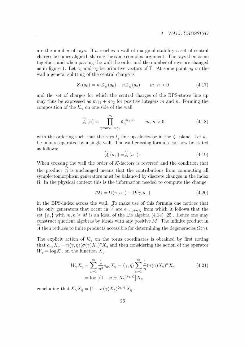
are the number of rays. If a reaches a wall of marginal stability a set of centralcharges becomes aligned, sharing the same complex argument. The rays then cometogether, and when passing the wall the order and the number of rays are changedas in figure 1. Let γ1 and γ2 be primitive vectors of Γ. At some point a0 on thewall a general splitting of the central charge is

Zγ(a0) = mZγ1(a0) + nZγ2(a0) m, n > 0 (4.17)

and the set of charges for which the central charges of the BPS-states line upmay thus be expressed as mγ1 + nγ2 for positive integers m and n. Forming thecomposition of the Kγ on one side of the wall

yA (u) ≡

y∏γ=mγ1+nγ2

KΩ(γ,a)γ m, n > 0 (4.18)

with the ordering such that the rays lγ line up clockwise in the ζ−plane. Let a±be points separated by a single wall. The wall-crossing formula can now be statedas follows: y

A (a+) =xA (a−) . (4.19)

When crossing the wall the order of K-factors is reversed and the condition that

the productyA is unchanged means that the contributions from commuting all

symplectomorphism generators must be balanced by discrete changes in the indexΩ. In the physical context this is the information needed to compute the change

∆Ω = Ω(γ, a+)− Ω(γ, a−) (4.20)

in the BPS-index across the wall. To make use of this formula one notices thatthe only generators that occur in

yA are emγ1+nγ2 from which it follows that the

set eγ with m,n ≥ M is an ideal of the Lie algebra (4.14) [25]. Hence one mayconstruct quotient algebras by ideals with any positive M . The infinite product inyA then reduces to finite products accessible for determining the degeneracies Ω(γ).

The explicit action of Kγ on the torus coordinates is obtained by first notingthat enγXη = n〈γ, η〉(σ(γ)Xγ)

nXη and then considering the action of the operatorWγ = logKγ on the function Xη

WγXη =∞∑n=1

1

n2enγXη = 〈γ, η〉

∞∑n=1

1

n(σ(γ)Xγ)

nXη (4.21)

= log[(1− σ(γ)Xγ)

〈η,γ〉]Xη

concluding that KγXη = (1− σ(γ)Xγ)〈η,γ〉Xη .

26

4 WALL-CROSSING

A few examples are in order to see how wall-crossing formulae behave and theinterpretation of them. Since the Xη are multiplicative it suffices to investigatethe transformation of the unit magnetic and electric functions respectively. Bydenoting X(1,0) = x and X(0,1) = y the KS symplectomorphism is

Kγ : (x, y) 7→(

(1− (−1)pqxpyq)q x, (1− (−1)pqxpyq)−p y)

(4.22)

for any charge γ = (p,q). By straightforward algebra one verifies the operatorequality

K(1,0)K(0,1) = K(0,1)K(1,1)K(1,0) (4.23)

which realises the general formula (4.19) when quoting the algebra by the ideal

P lγ1

lγ2

lγ1 = lγ1+γ2 = lγ2 lγ2

lγ1

lγ1+γ2

a = a+ a = a−a = aw

Figure 1: When a ∈ B crosses the wall the rays lγi corresponding to BPS states ofcharge γi rotate towards each other and their mutual ordering is eventually reverted.aw belongs to the wall of marginal stability and at this locus all rays coalesce to asingle ray. This example illustrates the behaviour of equation (4.23) where a boundstate of charge γ1 + γ2 is formed when a ∈ B follows a path a+ → a− that crossesthe wall.

given by m,n > 1. This is illustrated in figure 1. The physical interpretation ofthis formula is two BPS particles of unit magnetic and electric charge respectivelycoming together at a wall. When passing the wall one new dyonic charged particleis created. This is in accordance with results from supergravity investigations [10]where this extra bound state is found. A simililar result for the N = 2 theory withgauge group SU(3) was analysed in [4]. For the wall-crossing formula (4.23) theBPS index discontinuities ∆Ω(γ) = Ω(a+, γ)− Ω(a−, γ) are

∆Ω(1,0) = 0

∆Ω(1,1) = −1 (4.24)

∆Ω(0,1) = 0 .

27

5 COMPACTIFICATION TO THREE DIMENSIONS

In SU(2) Seiberg-Witten theory there is one wall of marginal stability separatingthe parameter space in a strong coupling and a weak coupling region. The wall-crossing phenomena is captured in the formula

K(2,−1)K(0,1) = (K(0,1)K(2,1)K(4,1) . . . )K−2(2,0)(. . .K(6,−1)K(4,−1)K(2,−1)) (4.25)

where the left hand side reflects the strong coupling spectrum - one monopole andone dyonic state. The exponents of both KS factors are 1 and hence these belongto the hypermultiplet. The right hand side represents the weak coupling side ofthe wall, where an infinite sequence of hypermultiplet states of dyonic chargesreside. The ’middle’ factor K−2

(2,0) corresponds to a state in the vector multiplet

since Ω = −2, recall equation (4.5). This state has charge (2,0) and is thus avector boson since the vector multiplet scalars are all neutral.

5 Compactification to Three Dimensions

In this section we compactify one direction of the four dimensional theory on acircle, keeping the circle radius as a parameter. An effective three dimensionaltheory is obtained in the small radius limit. We describe how the dimensionalreduction is performed reaching a N = 4 sigma model for the scalars. The vectorfield is dualised to two scalars in three dimensions and the moduli space geometry isrestricted to be a hyperkahler manifoldM. The rest of this section is devoted to theexplicit description of the geometry, starting from the Gibbons-Hawking ansatz.With a compactified direction there is a tower of field excitations on the circlewhich contributes to the metric. It is described how these instanton correctionsare accounted for in a twistor space construction of the metric. This approachis the one used in [13] to formulate a Riemann-Hilbert problem for the Darbouxcoordinates onM. The continous solution for this problem is then shown to be inone-to-one correspondence with a KS wall-crossing formula for the BPS-index.

5.1 The Bosonic Field Content

Compactifying the theory on S1 will give an effective theory in three dimensionswith the circle radius R as a parameter. The gauge field AI splits to a threedimensional 1-form AI(3) and a scalar AI4 upon compactification. The two-formfield strength in three dimensions is Hodge dual to a 1-form field strength of a realscalar field. Thus each gauge field will give rise to two real scalar fields and since

28


there are one gauge field to each complex scalar aI in the vector multiplet thisdoubles the dimension of the moduli space.

By imposing that the fields of (2.27) not depend on the fourth coordinate x4 weget the splitting

d4aI → daI(xi) AI → AI(3) + AI4(xi)dx4 F I → F I

(3) + dAI4 ∧ dx4 (5.1)

where all exterior derivatives on the right hand side are three dimensional, a con-vention which is used from now on. The metric on R1,2 × S1 is g = dxi ⊗ dxi +R2dx4 ⊗ dx4 with Lorentzian signature and i = 0,1,2. Under the splitting (5.1)the kinetic terms become

daI ∧ ∗daJ → Rdx4 ∧ daI ∧ ∗daJ (5.2)

F I ∧ ∗F J → Rdx4 ∧ F I(3) ∧ ∗F J

(3) +1

Rdx4 ∧ dAI4 ∧ ∗dAJ4

and all quantities on the right hand side are three dimensional. We also note herethat ∗∗ = −1 on two-forms in three dimensional Minkowski space which will beused in the following calculations.

Inserting the splitted fields in the Lagrangian (2.27) and integrating out the S1

direction gives

L(3) = − 1

4π

∫S1

[dx4 ∧ = τIJ(R daI ∧ ∗daJ +

1

RdAI4 ∧ ∗dAJ4 (5.3)

+RF I(3) ∧ ∗F J

(3)) + 2dx4 ∧ < τIJF I(3) ∧ dAJ4

]= −1

2

[= τIJ(R daI ∧ ∗daJ +

1

RdAI4 ∧ ∗dAJ4

+RF I(3) ∧ ∗F J

(3)) + 2< τIJF I(3) ∧ dAJ4

]since the x4 periodicity is 2π. The gauge field A(3) is dualised to a magnetic scalarΛI by adding a Lagrange multiplier term F I

(3) ∧ dΛI . This term is exact and willnot change the equations of motion. Then the Euler-Lagrange equations

0 = δFL = δF I(3) ∧

(−R=τIJ ∗ F J

(3) −< τIJdAJ4 + dΛI

)(5.4)

⇒ ∗F J(3) =

1

R(= τ)−1,IJ (dΛI −< τIJdAJ4 )

allow us to rephrase the Lagrangian in terms of Λ instead of A(3). By replacing allfield strengths F I

(3) = − ∗ (∗F I(3)) in (5.3) eliminates the field strength in favor of

the introduced scalar field.

29


To be consistent with the notation of [13] we introduce the magnetic and electriccoordinates θm,I = ΛI/2π and θIe = AI4/2π of periodicity 1. These are the ’electric’and ’magnetic’ Wilson lines over the circle dimension

θIe =

∫S1

AI4 dx4 θm,I =

∫S1

(A∗(3))Idx4 (5.5)

where (A∗(3))I are the scalars dual to the three-dimensional gauge fields. This is not

the scalars ΛI , which are obtained after truncating the dependence on x4. Aftersome simplification the Lagrangian takes the form

L(3) = −1

2

R= τIJdaI ∧ ∗daJ (5.6)

+1

4π2R(= τ−1)IJ(dθm,I − τIKdθKe ) ∧ ∗(dθm,J − τJLdθLe )

.

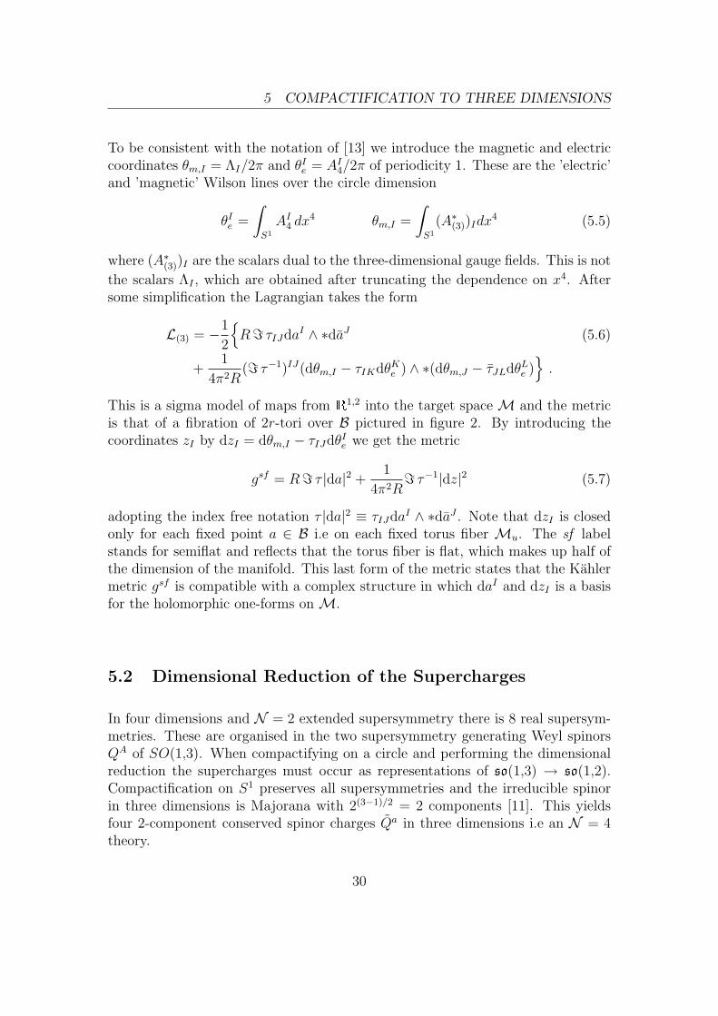
This is a sigma model of maps from R1,2 into the target space M and the metric

is that of a fibration of 2r-tori over B pictured in figure 2. By introducing thecoordinates zI by dzI = dθm,I − τIJdθIe we get the metric

gsf = R= τ |da|2 +1

4π2R= τ−1|dz|2 (5.7)

adopting the index free notation τ |da|2 ≡ τIJdaI ∧ ∗daJ . Note that dzI is closedonly for each fixed point a ∈ B i.e on each fixed torus fiber Mu. The sf labelstands for semiflat and reflects that the torus fiber is flat, which makes up half ofthe dimension of the manifold. This last form of the metric states that the Kahlermetric gsf is compatible with a complex structure in which daI and dzI is a basisfor the holomorphic one-forms on M.

5.2 Dimensional Reduction of the Supercharges

In four dimensions and N = 2 extended supersymmetry there is 8 real supersym-metries. These are organised in the two supersymmetry generating Weyl spinorsQA of SO(1,3). When compactifying on a circle and performing the dimensionalreduction the supercharges must occur as representations of so(1,3) → so(1,2).Compactification on S1 preserves all supersymmetries and the irreducible spinorin three dimensions is Majorana with 2(3−1)/2 = 2 components [11]. This yieldsfour 2-component conserved spinor charges Qa in three dimensions i.e an N = 4theory.

30


B

M

a

Ma

θe

θm

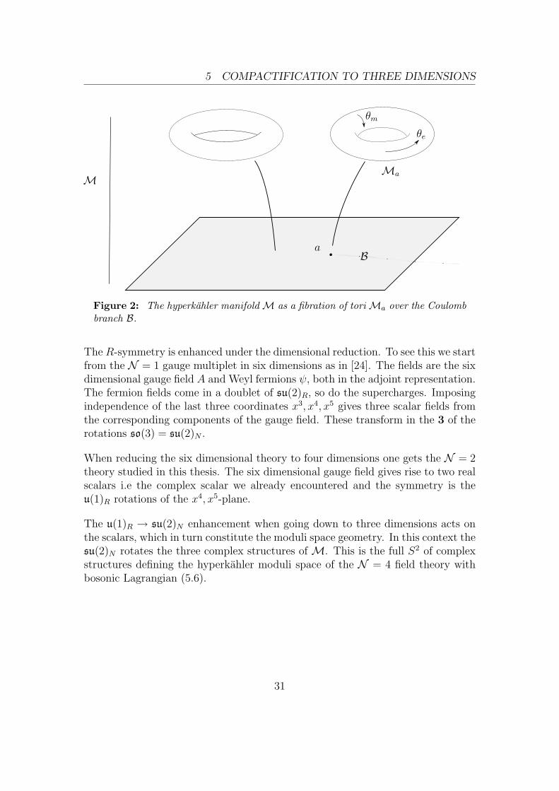
Figure 2: The hyperkahler manifoldM as a fibration of toriMa over the Coulombbranch B.

The R-symmetry is enhanced under the dimensional reduction. To see this we startfrom the N = 1 gauge multiplet in six dimensions as in [24]. The fields are the sixdimensional gauge field A and Weyl fermions ψ, both in the adjoint representation.The fermion fields come in a doublet of su(2)R, so do the supercharges. Imposingindependence of the last three coordinates x3, x4, x5 gives three scalar fields fromthe corresponding components of the gauge field. These transform in the 3 of therotations so(3) = su(2)N .

When reducing the six dimensional theory to four dimensions one gets the N = 2theory studied in this thesis. The six dimensional gauge field gives rise to two realscalars i.e the complex scalar we already encountered and the symmetry is theu(1)R rotations of the x4, x5-plane.

The u(1)R → su(2)N enhancement when going down to three dimensions acts onthe scalars, which in turn constitute the moduli space geometry. In this context thesu(2)N rotates the three complex structures of M. This is the full S2 of complexstructures defining the hyperkahler moduli space of the N = 4 field theory withbosonic Lagrangian (5.6).

31


5.3 Describing the Hyperkahler Geometry

The following subsections are devoted to reproducing the metric (5.7) from a hy-perkahler metric ansatz. First we consider the classical, or semi-flat, metric validin the large radius limit. Then we describe how corrections to this metric dueto instantonic excitations along the compact direction is accounted for. Somebackground on hyperkahler geometry is reviewed in appendix A.

5.3.1 The Semiflat Metric

We now describe how the semiflat hyperkahler geometry with metric gsf may beobtained using the twistor space construction which is introduced in appendixA. The twistor space Z = M × P is topologically the trivial fibration of thehyperkahler manifold M over the complex projective line P. The projection π :Z → P is the map π(u, ζ) = ζ for u ∈M and ζ ∈ P is the twistor parameter.

In the twistor approach Darboux coordinates ξ on the twistor space Z are searchedfor, such that

ϑ =1

4π2Rdξm ∧ dξe (5.8)

is a section of Ω2Mζ⊗OP(2). The prefactor (4π2R)−1 is due to the chosen notation.

This ϑ(ζ) is a holomorphic symplectic form for each fiber Mζ = π−1(ζ), that is,ϑ(ζ) is a (2,0)-form in the complex structure Jζ for each fixed ζ ∈ P. As a sectionof the line bundle OP(2) ϑ is a section defined as a second degree polynomial in ζ(with the proper transition functions between the patches of P). The three Kahlerforms onM are ω± = ω1 ± iω2 and ω3 and the symplectic form on Z is expressedas

ϑ(ζ) = − i

2ζω+ + ω3 −

iζ

2ω− . (5.9)

At ζ = 0 and ζ =∞ this form is to be multiplied with the OP transition functionsζ and ζ−1 respectively.

The semiflat Darboux coordinates have a neat realisation in terms of the centralcharge Z and the gauge field Wilson lines θ. When no instanton contributions areconsidered they are given by

ξγ = πRζ−1Zγ + iθγ + πRζZγ (5.10)

and in the following we will see that they reproduce the semiflat hyperkahlergeometry (5.7). In the work of [13] the concept of ’Darboux functions’ X are

32


introduced as the exponentiations

Xγ = exp(ξγ) (5.11)

of the Darboux coordinates which turns out to be convenient in the wall-crossingcontext, treated in section 6. The holomorphicity of ξ, X or ϑ for each fixed ζ maybe phrased in terms of the Cauchy-Riemann equations overM [13]. In appendix Athe holomorphicity of ϑ over M in complex structure Jζ is shown explicitly. Thesemiflat moduli space metric of the compactified theory has a simple realisation interms of the Darboux functions. Collecting the magnetic and electric coordinatesas θ = θIeαI − θm,IβI the Darboux functions

X sfγ (ζ) = exp[πRζ−1Zγ + iθγ + πRζZγ] (5.12)

are defined. Computing the holomorphic symplectic form using the special Kahlercondition (2.38) gives

ϑsf (ζ) =1

8π2R〈γi, γj〉−1d logX sf

γi(ζ) ∧ d logX sf

γj(ζ) (5.13)

=1

4π

[iζ−1〈dZ, dθ〉+

(πR〈dZ, dZ〉 − 1

2πR〈dθ, dθ〉

)+ iζ〈dZ, dθ〉

].

Comparing this expression with (5.9) the Kahler form ω+ is extracted as

ω+ = − 1

2π〈dZ, dθ〉 = − 1

2π〈dXIαI − dFIβ

I , dθJe αJ − dθm,JβJ〉 (5.14)

=1

2π(daI ∧ dθm,I −

∂2F(a)

∂aI∂aJdaI ∧ dθJe ) =

1

2πdaI ∧ dzI

by choosing a duality frame. In appendix A it is shown how the complex structureJsf3 may be calculated from this Kahler form. The terms independent of ζ in (5.13)constitute the Kahler form

ωsf3 =R

4〈dZ, dZ〉 − 1

8π2R〈dθ, dθ〉 (5.15)

in the third complex structure. Again, by choosing a duality frame this Kahlerform is rewritten in the coordinates aI , zI as

ωsf3 =i

2

(R(= τ)IJdaI ∧ daJ +

1

4π2R(= τ)−1,IJdzI ∧ dzJ

), (5.16)

which states that in Jsf3 the metric gsf is Kahler with the Kahler form given above.It follows that this is the hyperkahler metric as obtained from the compactificationon S1 (5.6).

33


5.3.2 The Ooguri-Vafa Metric

When compactifying on a circle one introduces the possibility for field excitationsaround the compact direction which are referred to as instanton contributions.BPS states of mass M = |Z| wrapping a circle of radius R are exponentiallysupressed by e−|Z|R as the radius goes to infinity. Their action is ∼ |Z|R andhence the partition function gets the exponential supression. In this limit thereare no contribution from winding states and the semiflat metric is the classical one.The opposite limit, when R→ 0 was identified as the Atiyah-Hitchin manifold inthe case of a SU(2) theory [24].

In the following we are interested in the region where R is not small. In this casethe contributions from all the BPS states in the four-dimensional theory must beaccounted for and this will lead to the wall-crossing phenomenon. For arbitraryfinite R one may expect contributions from the wrapped excitations to the metric.In the following we describe how to take this into account in a simplified case.Given a number of charged particles that are all mutually local it is possible tochoose a duality frame where all particles are electrically charged [22]. To start withwe restrict the treatment to the case of one particle of electric charge γ = (0, q).

Recall that the moduli space M is a torus fibration over the Coulomb branch B.Without coupling to some charged particles the magnetic and electric coordinatesof the torus in are invariant under a U(1)m×U(1)e action of shift symmetry alongthe torus directions. When introducing a electrically charged particle the isometryin the electrical coordinate are broken while shifts of the magnetic coordinates stillare isometries.

The Gibbons-Hawking ansatz describes a family of hyperkahler metrics with a U(1)isometry. In this first example we consider the rank 1 case and we take coordinates(x1, x2, x3) with a = x1 + ix2 and θe = 2πRx3. For the isometry Killing vector ∂θmthe Gibbons-Hawking form of the metric is

g = V −1(x)(dθm2π

+ A(x))2 + V (x)dxi ⊗ dxi (5.17)

for A the U(1) connection and V obeying

dA = ∗dV (5.18)

making V the dual scalar potential to the connection. Given this form of themetric three Kahler forms are obtained as

ωa = dxa ∧ (dθm + A) +V

2εabcdxb ∧ dxc (5.19)

34


giving the hyperkahler structure to the geometry on M specified by g. These areclosed due to the condition (5.18) and it follows that V is harmonic, [15]. To givean explicit expression for the Gibbons-Hawking form of the metric some physicalconstraints are needed.

First of all the metric should reduce to the semiflat metric when instanton contri-butions are suppressed and R → ∞. The singular point in this example is a = 0where the BPS-states become massless and the full gauge group is restored. Hencefor |a| → ∞ the limit of g must be gsf . The wanted metric is periodic in θe andhave no continuous shift invariance along this direction. Also, the semiflat metricis invariant under rotations of a which suggests that the full metric is just a func-tion of |a| and the torus coordinates. As concluded in [22] these constrains have aunique solution (up to a possible integration constant) which in our notation takesthe form

V (a, θe) =q2R

4π

∞∑n=−∞

1√q2R2|a|2 + ( qθe

2π+ n)2

− bn (5.20)

with some bn of order 1/|n| introduced for convergence.

This potential contains all contributions to the metric, with the semiflat metricas the zero mode. In extracting this mode it is convenient to perform a Poissonresummation of this expression. Starting from the identity

1

|x|=

∫ ∞0

dt

t3/2exp[−π

t|x|2] (5.21)

and for simplicity defining the denominator expression√q2R2|a|2 + (

qθe2π

+ n)2 ≡ |y|, y = y1 + i(y2 + n) (5.22)

the potential is rewritten

V =

∫ ∞0

dt

t3/2exp[−π

ty2

1]∞∑

n=−∞

exp[−πt

(y2 + n)2] . (5.23)

By employing the Poisson resummation formula

∞∑n=−∞

f(n) =∞∑

k=−∞

f(2πk) for f(ω) =

∫ ∞−∞

f(x)eiωxdx (5.24)

V may be rewritten as

V =

∫ ∞0

dt

t3/2exp[−π

ty2

1]√t∞∑

n=−∞

exp[−πtn2 − 2πiy2n] (5.25)

35


and the occurence of the factor 2π in the resummation formula is due to the choiceof Fourier transform convention. Extracting the oscillating term in the equationabove, which is independent of the integration parameter, gives the Bessel integral

V =∞∑

n=−∞

exp[−2πiy2n]

∫ ∞0

dt

texp[−π

ty2

1 − πtn2] = (5.26)

= 2∞∑

n=−∞

exp[−2πiy2n]K0(2π|y1n|) .

The modified Bessel functionK0(x) has the asymptotic behaviourK0(x) ∼ − log(x/c)for small x and for some constant c. The zero mode may be viewed as the |a| → 0behaviour of K0 for some non-zero n. The choice of regularization bn will contributeto this constant and they are treated collectively as the constant Λ. Inserting theexpressions for y1, y2 and the prefactor gives the final expression

V = V sf + V inst = −q2R

4πlog(

aa

ΛΛ) +

q2R

2π

∑n6=0

exp[iqθen]K0(2πR|qan|) (5.27)

and the Λ is to be interpreted as the energy scale. The Bessel function in (5.27)has a large argument expansion in which the leading behaviour is K0(2π|a|R) ∼e−2πR|a| for large R and a, as expected for instanton contributions. The classicalmetric is obtained in the region far away from the singular point |a| = 0 as wellas in the decompactification limit. The exponential in θe breaks the translationalinvariance from R to Z as expected in the presence of an electric charge. Theconnection dual to the potential V in (5.18) is given by A = Asf + Ainst with

Asf =iq2

8π2

(log

a

Λ− log

a

Λ

)dθe (5.28)

Ainst = −q2R

4π

(da

a− da

a

)∑n6=0

sgn(n) exp[iqθen]|a|K1(2πR|qan|) .

The semiflat contribution is singular at a = 0 and taking the corrections intoaccount we see that the possible singularities is a = 0, θe = 2πn/q. The secondcondition has q solutions while θe is 2π-periodic. The four dimensional spacewith coordinates (a, θm, θe) is locally C2, and subject to the identification θe ∼θe + 2πn/q. The space in the vicinity of a = 0 is then the quotient space C2/Zqi.e an Aq−1 singularity. In the special case of q = 1 there is no singularity and thespace is perfectly smooth.

36


5.3.3 Twistor Space Description

In this section we make connection with section 5.3.1 and describe how to extendthe twistor construction of the semiflat case to the instanton corrected metric. Theholomorphic symplectic form ϑ over the twistor space M×P is obtained as

ϑ(ζ) =1

4π2Rdξm ∧ dξe (5.29)

for ξm,e the magnetic and electric Darboux coordinates whose differentials are

dξm = idθm + 2πiA(x) + iπV (x)(ζ−1da− ζda

)(5.30)

dξe = idθe + πR(ζ−1da+ ζda

).

The holomorphic 2-form ϑ is an element of Ω(2,0)(M) for each ζ ∈ P in complexstructure Jζ . This implies that both Darboux coordinate differentials are of type(1,0) i.e holomorphic one forms in Jζ .

Taking ξe = logXe and using that the electric unit charge is γ = (0,1) gives Zγ asthe coordinate a ∈ B and θγ = θe. Written out ξe is

ξe = πRζ−1a+ iθe + πRζa (5.31)

which is the same expression as in (5.10). The conclusion is that the electric coor-dinate contribution to the symplectic form is the classical one and the instantoncorrections are all in the magnetic coordinate ξm. The problem of finding theinstanton corrected Darboux functions over the twistor space is thus restrictedto finding the magnetic solution. The straightforward way would be to make anansatz for Xm and then solve the corresponding Cauchy-Riemann equations onM.

In [13] a different approach is presented for the solution, and instead of demandingholomorphicity given the geometry they look for a solution that is validated bygiving the right symplectic form ϑ. By linearity the splitting in semiflat andinstanton corrected contributions are transferred to the symplectic form as

ϑ(ζ) = ϑsf (ζ) + ϑinst(ζ)

ϑsf (ζ) = − 1

4π2Rdξe ∧

[idθm + 2πiAsf + πiV sf (ζ−1da− ζda)

](5.32)

ϑinst(ζ) = − 1

4π2Rdξe ∧

[2πiAinst + πiV inst(ζ−1da− ζda)

]identifying dξsfm as the right factor of the second line. In the semiflat part abovethe term Asf ∼ dθe carries a dependence on the electric torus coordinate θe. In

37


constructing the Darboux functions with the origin in the magnetic-electric dualityframe we want to separate the dependence on θm and θe. The solution to thisis to simply subtract a multiple of the electric coordinate dξe such that the θedependence cancels. This maneuver preserves the symplectic form

ϑsf ∼ dξe ∧ (dξsfm − kdξe) = dξe ∧ dξsfm (5.33)

and the explicit semiflat magnetic coordinate is

dξsfm = idθm + 2πiAsf + πiV sf (ζ−1da− ζda)− iq2

4π

(log

a

Λ− log

a

Λ

)dξe

=Rq2

2iζ−1d(a log

a

Λ− a) + idθm −

Rq2

2iζd(a log

a

Λ− a) . (5.34)

where we recognise the multiple of dξe as the rightmost term in the first line. Thisexpression coincides with the ansatz (5.12) for a unit magnetic charge γ = (1,0),

and for the central charge function Zm = q2

2πi(a log a

Λ− a).

The form of the instanton-corrected magnetic solution worked out in [13] is theingenious ansatz

Xm = X sfm exp

[ iq4π

∫l+

dη

η

η + ζ

η − ζlog[1−Xe(η)q] (5.35)

− iq

4π

∫l−

dη

η

η + ζ

η − ζlog[1−Xe(η)−q]

]where the paths l± are any paths from 0 to ∞ on P belonging respectively to thehalf-planes

H± = ζ : ±< aζ< 0 (5.36)

which are viewed as two hemispheres of P. The two contours are to be read as thecontributions from positively and negatively winded state excitations around S1.The verification of the ansatz (5.35) reduce to checking that

ϑ(ζ) = − 1

4π2Rd logXe ∧ d logXm (5.37)

reproduces the symplectic form (5.29) corresponding to the Ooguri-Vafa metric.The differential of the magnetic Darboux coordinate is

d logXm = d logX sfm + I+ + I− (5.38)

38


for the integrals

I± = ± iq4π

d(∫

l±

dη

η

η + ζ

η − ζlog[1−Xe(η)±q]

)= ± iq

4π· ∓q

∫l±

dη

η

η + ζ

η − ζX±qe (η)

1−X±qe (η)

dXe(η)

Xe(η)(5.39)

= −iq2

4π

∫l±

dη

η

η + ζ

η − ζX±qe (η)

1−X±qe (η)d logXe(η) ,

remembering that theP parameter ζ is constant with respect to the exterior deriva-tive. The expression (5.38) and the splitting (5.32) implies that the correction partmust obey

d logXe ∧ (I+ + I−) = d logXe ∧[2πiAinst + πiV inst(ζ−1da− ζda)

]. (5.40)

This is the equation that we verify by evaluating the left hand side. To performthe integrals we deform the contours l± to the specific case

l± = η : ±aη∈ R− (5.41)

which are the two rays centered on the half planes H±. First we note that themodulus of the electric Darboux function

|Xe(η)| < 1 ∀ η ∈ l+ (5.42)

since the real part of ξe is strictly negative on this path. The analogous statementis that |Xe| > 1 on l−. The wedge products on the left in (5.40) may be rewrittenby moving the one form under the integral yielding the expression

η + ζ

η − ζd logXe(ζ) ∧ d logXe(η) =

η + ζ

η − ζd logXe(ζ) ∧ [d logXe(η)− d logXe(ζ)]

= πRη + ζ

η − ζd logXe(ζ) ∧

[(η−1 − ζ−1)da+ (η − ζ)da

](5.43)

= −πR d logXe(ζ) ∧[(η−1da− ηda) + (ζ−1da− ζda)

]which contains terms of order −1, 0 and 1 in η. Inserting this expression in (5.40)gives the integrals

iq2R

4d logXe(ζ) ∧

∫l+

dη

η

[(η−1da− ηda) + (ζ−1da− ζda)

] X qe (η)

1−X qe (η)

+

∫l−

dη

η

[(η−1da− ηda) + (ζ−1da− ζda)

] X−qe (η)

1−X−qe (η)

(5.44)

39


which may be evaluated in closed form. We consider the different orders of ηseparately. The l+-integral over the ζ- and ζ−1-terms is

(ζ−1da− ζda)

∫l+

dη

η

X qe (η)

1−X qe (η)

(5.45)

and since the modulus of the Darboux function is less than one we may rewrite theintegral part above as a geometric series. This allows for moving out the oscillatingθe-factor leaving a Bessel integral∫

l+

dη

η

X qe (η)

1−X qe (η)

=

∫l+

dη

η

∑n>0

X qne (η)

=∑n>0

exp[iqnθe]

∫l+

dη

ηexp[πRqn(

a

η+ ηa)] (5.46)

=∑n>0

exp[iqnθe]

∫R+

dx

xexp[−πRqn(

1

x+ x|a|2)]

= 2∑n>0

exp[iqnθe]K0(2πR|qan|) .

Over the ray l+ from 0 to ∞ the integral is evaluated as a real integral, changingvariable to x = η/a < 0 giving dη/η = dx/x. This ensures that the exponent isalways real and negative and hence a convergent Bessel integral. The correspondingintegral over l− gives by the same construction x > 0 and the negative sign is dueto the negative charge q over this ray. The geometric sum is thus effectively overthe negative integers and together the integrals contribute by

iq2R

2d logXe(ζ) ∧ (ζ−1da− ζda)

∑n6=0

exp[iqnθe]K0(2πR|qan|) = (5.47)

d logXe(ζ) ∧ iπV inst(ζ−1da− ζda)

to (5.40). To evaluate the integrals multiplying the (η−1da− ηda) factor in (5.44)we treat first the l+-case. The first integral is

da

∫l+

dη

η2

X qe (η)

1−X qe (η)

= da

∫l+

dη

η2

∑n>0

X qne (η) =

da∑n>0

exp[iqnθe]

∫l+

dη

η2exp[πRqn(

a

η+ ηa)] (5.48)

= −2 da∑n>0

|a|a

exp[iqnθe]K1(2πR|qan|)

40


where we picked up a total minus sign from the dη/η2-term which is negative forthe l+-ray and the factor of |a| is due to the Bessel integral. In the same spirit thesecond integral (of order η in (5.44)) is evaluated to

da

∫l+

dη

ηηX qe (η)

1−X qe (η)

=

da∑n>0

exp[iqnθe]

∫l+

dη exp[πRqn(a

η+ ηa)] (5.49)

= −2 da∑n>0

|a|a

exp[iqnθe]K1(2πR|qan|) .

Adding the results of the ray l−, with sums over negative integers, and an overallsign due to the positiveness of the integral parameter the result is

− iq2R

2d logXe(ζ) ∧

∑n6=0

sgn(n)|a| exp[iqnθe]K1(2πR|qan|) (5.50)

= d logXe(ζ) ∧ 2πiAsf

which completes the check that the ansatz actually gives the magnetic functionthat reproduces the metric. Comparing (5.40) to the integral contributions (5.47)and (5.50) we see that all instanton contributions agree.

We note here that the generalisation to higher rank, or manifolds of higher dimen-sion, is carried out following the same line of reasoning. In coordinates xI = (aI , θIe)and θm,I chosen such that the U(1)r isometry Killing vectors are ∂θm,I the metricis

g = V (x)−1,IJ(dθm,I

2π+ AI(x))(

dθm,J2π

+ AJ(x)) + V (x)IJdxI · dxJ (5.51)

and to keep the hyperkahler structure the relation between AI and VIJ are chosensuch that the Kahler forms

ωa = dxa,I ∧ (dθm,I + AI) +1

2VIJε

abcdxb,I ∧ dxc,J (5.52)

all are closed, in accordance with the existence of the Kahler forms (5.19). Analo-gous expressions for the potentials V and A are obtained and it is found that theelectric Darboux functions are the semiflat ones. The instanton corrections areaccounted for in the magnetic functions. Details of these calculations are found in[13].

41

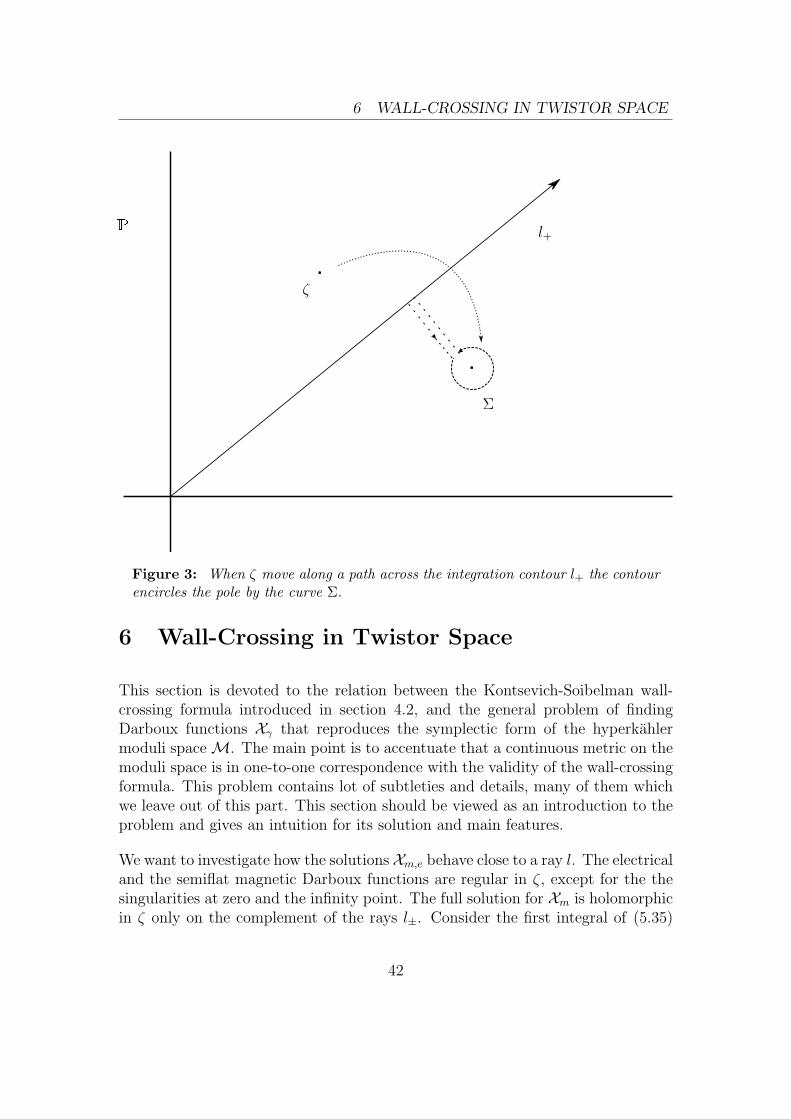
6 WALL-CROSSING IN TWISTOR SPACE

P l+

ζ

Σ

Figure 3: When ζ move along a path across the integration contour l+ the contourencircles the pole by the curve Σ.

6 Wall-Crossing in Twistor Space

This section is devoted to the relation between the Kontsevich-Soibelman wall-crossing formula introduced in section 4.2, and the general problem of findingDarboux functions Xγ that reproduces the symplectic form of the hyperkahlermoduli spaceM. The main point is to accentuate that a continuous metric on themoduli space is in one-to-one correspondence with the validity of the wall-crossingformula. This problem contains lot of subtleties and details, many of them whichwe leave out of this part. This section should be viewed as an introduction to theproblem and gives an intuition for its solution and main features.

We want to investigate how the solutions Xm,e behave close to a ray l. The electricaland the semiflat magnetic Darboux functions are regular in ζ, except for the thesingularities at zero and the infinity point. The full solution for Xm is holomorphicin ζ only on the complement of the rays l±. Consider the first integral of (5.35)

42


and let ζ follow a path crossing the ray l+ clockwise. When crossing the contour ofintegration the pole of the integrand crosses the ray as well and hence the integralmay be splitted ∮

l+

→∮l+

+

∮Σ

(6.1)

where Σ is a closed positively oriented curve enclosing the pole on the other side ofthe curve, as in figure 3. The limits when ζ → l+ clockwise and counterclockwiserespectively are denoted (Xm)±l+ and correspondingly for the path l−. Due to theexponent in the solution (5.35) the contribution from the Σ-integral is multiplica-tive. By the residue theorem the closed contour integral is

iq

4π

∮Σ

dη

η

η + ζ

η − ζlog[1−Xe(η)q] = 2πi

iq

4π· ζ + ζ

ζlog[1−Xe(ζ)q]

= log(1−Xe(ζ)q)−q (6.2)

and the contribution to Xm is thus (1 − Xe(ζ)q)−q. Equating the expressions onboth sides of the rays yields

(Xm)+l+

= (Xm)−l+(1−Xe(ζ)q)−q (6.3)

and the corresponding expression

(Xm)+l−

= (Xm)−l−(1−Xe(ζ)−q)q (6.4)

for the path l−. We see that these expressions resembles the behaviour of the toruscoordinates Xm,e under the KS transformation introduced in section 4.2. In thefollowing we make this relation precise.

The functions Xm and Xe constitutes, for fixed values of a,R and ζ, a map

X :Ma → Ta (6.5)

whereMa is the torus fiber of the hyperkahler fibrationM→ B with coordinates(θm, θe). One may restate the relation, saying that Xγ is the pullback Xγ(θ) =Xγ(X (θ)) to the torus fiber Ma of the coordinates Xm,e. Ta is a complexifiedtorus with coordinates (Xm, Xe) introduced in section 4.2. As functions on the fiberXm,e = exp[i(θm,e + f(θ))] where f is due to possible monodromy transformationsaround a = 0. They both hence take S1-values and this is the reason for the map(6.5) to take values on a torus Ta.

The solutions X are valued on the torus Ta and hence the KS transformations(4.22) apply to the Darboux functions. Actually the discontinuities of Xm in (6.3)-(6.4) may be stated as

X+m = K(±q,0)X−m (6.6)

43


at the rays l±. This is the link between the work of Kontsevich and Soibelman andthe description of the moduli space in the simplest case. The description of theDarboux coordinates over M has necessarily discontinuities, which are accountedfor as KS transformations. So far we have considered mutually local particles andwe now turn to the general case.

We now turn to the case where not all particles are mutually local i.e there is noduality frame where all particles may be considered electrically charged. As in theprevious case the full hyperkahler metric g receives corrections from instantonsoriginating from massive BPS states in four dimensions. The contribution fromeach BPS state of charge γ are expected to be weighted by the BPS index Ω(γ).From section 4.1 we know that these degeneracies are only piecewise constant overthe base B. Hence the instanton corrections have discontinuous jumps at some locion the Coulomb branch and so should the full metric.

From the Lagrangian of the compactified theory we expect the metric g to be ev-erywhere smooth, since it is specified by the holomorphic period matrix τ . Thetower of instanton contributions and their discontinuities must therefore be care-fully balanced so to make g smooth. The authors of [13] found that this is achievedif the BPS index obey the Kontsevich-Soibelman wall-crossing formula. This state-ment is at the heart of the physical interpretation of the wall-crossing formula. Inthe following we motivate why this has to be true.

A Riemann-Hilbert problem is the problem of finding holomorphic functions f+(z)and f−(z) on the interior and exterior respectively of a closed curve Σ. For allz ∈ Σ they obey a boundary condition α(z)f+(z) + β(z)f−(z) = γ(z) for somegiven holomorphic functions α, β and γ.

This is the precise setup needed to describe the Darboux functions as piecewiseanalytic over the full manifold M. The KS symplectomorphisms are maps

Kγ : Ta → Ta (6.7)

which for charges that support BPS states gives contribution to the wall-crossingformula. To make contact with the contours l of the solution (5.35) for the magneticDarboux function the subset

Γa,l = γ ∈ Γa |Zγ(a)/ζ ∈ R− , ζ ∈ l (6.8)

of the local charge lattice Γa is defined. The rays where Γa,l 6= ∅ are named BPSrays. The corresponding transformation

Sl =∏γ∈Γa,l

KΩ(γ)γ (6.9)

44


over BPS states is thus over all possible charges whose central charges line up alongthe ray l. If the set Γa,l is empty then Sl is 1. Note that this is very similar to

the construction ofyA in section 4.2. However for γ ∈ Γa,l all KS transformations

commute, since the charges in this subset are all real multiples of each other. Thisgives 〈γ, γ′〉 = 0 and thus the Lie algebra generators all commute from which itfollows that no particular ordering of the operator product need to be stated.

The boundary condition of the Riemann-Hilbert problem over the ray l is set to

X+ = SlX− (6.10)

where X± are the limits of X when ζ approaches l clockwise or counterclockwiserespectively. This is the generalisation of the discontinuity over l for the unit chargefunctions Xm,e in (6.6). For each ray where the central charges share their complexargument a Riemann-Hilbert problem is formulated as above. The solutions arepiecewise holomorphic functions of ζ away from the rays.

So far the discussion of the solution has been about the ζ-dependence of the Dar-boux functions. The metric is not dependent on the twistor parameter and wewant to say something about the solutions as functions on M. Away from themarginal stability walls in B the solutions are continuous since the BPS spectrumis constant at these loci. Let a0 be any point on the wall and consider the casewhen a ∈ B approaches this wall from one side. The BPS rays corresponding tocharges γ = mγ1 + nγ2 will rotate towards each other eventually approaching asingle ray while keeping their mutual ordering. The Riemann-Hilbert discontinuityof X at the wall is thus

yA =

y∏γ=mγ1+nγ2

KΩ(γ,a+)γ m, n > 0 (6.11)

and if the limit lima→a0 X exists from this side of the wall it is a solution tothe Riemann-Hilbert problem at the ray l. If one makes the same argument, butconsider a approaching the wall from the other side gives a analogous discontinuity,but with the product in the reverse order. X is continuous at a0 if the two limitsagree at this point and is thus the solution to the same Riemann-Hilbert problem.Recall that the wall-crossing formula (4.19) is precisely this statement if X iscontinuous over the wall of marginal stability.

The full instanton corrected Darboux functions are solutions to the integral equa-tion

Xγ(ζ) = X sfγ exp

[− 1

4πi

∑γ′

Ω(γ′, a)〈γ, γ′〉∫lγ′

dη

η

η + ζ

η − ζlog1− σ(γ′)Xγ′(η)

],

45


which is a crucial part of the main result of Gaiotto, Moore and Neitzke in [13].If the Kontsevich-Soibelman wall-crossing formula is satisfied by the BPS indexthere is an piecewise analytic solution in a and ζ for the Darboux functions overM. It follows that the metric constructed out of the symplectic form on thehyperkahler manifold is continuous. The transformations Kγ over the wall are allsymplectomorphisms and hence they are compatible with differentiable transitionfunctions gluing the charts of M together to a manifold.

46

A HYPERKAHLER GEOMETRY

Appendices

A Hyperkahler Geometry

In appendix A.1 a brief background on hyperkahler geometry is presented. Thebasic ingredients and relations are introduced on a working level for applicationin section 5. In A.2 the construction of a hyperkahler geometry via Darbouxcoordinates are introduced. Making use of the full Riemann sphere of complexstructures and the symplectic form on the manifold allows for Darboux coordinatefunctions X (u, ζ) with certain properties, all used in section 5, and presented inpart two of this appendix. See e.g [17].

A.1 Foundations

A hyperkahler manifold M is a Riemannian manifold of 4n real dimensions. Itcarries three covariantly constant complex structures J1, J2 and J3 giving threedifferent Kahler forms ω1, ω2 and ω3 respectively. The complex structures are(1,1) tensor fields obeying the quaternion algebra

JaJb = −δab + εabcJc . (A.1)

The space of Kahler metrics is infinite dimensional since a Kahler metric may betransformed to another Kahler metric by adding any function f(z, z) ∈ C∞ tothe Kahler potential. The set of hyperkahler geometries are much more restricted,since a Kahler transformation has to preserve the compatibility with all complexstructures and it is known that the set of isometry classes is finite [16]

For any point (a1, a2, a3) ∈ S2 we may form the linear combination aiJi which isalso a covariantly constant complex structure on M since

(aiJi)2 = aiajJiJj = −aiai = −1 (A.2)

and where the cross terms vanish due to antisymmetry. The map

a1 = iζ − ζ1 + ζζ

a2 = − ζ + ζ

1 + ζζa3 =

1− ζζ1 + ζζ

(A.3)

realises the isomorphism S2 ≈ CP1 = P. Hence we have a family of complex

structures and corresponding Kahler forms, parametrised by a complex parameter

47


ζ ∈ P and

Jζ = − 1

1 + ζζ

(i(ζ − ζ)J1 − (ζ + ζ)J2 + (1− ζζ)J3

)(A.4)

= − 1

1 + ζζ

(iζJ+ − iζJ− + (1− ζζ)J3

)for J± = J1 ± iJ2. We will consider the form

ϑ(ζ) = − i

2ζω+ + ω3 −

iζ

2ω− (A.5)

where correspondingly ω± = ω1 ± iω2. At the points 0 and ∞ of the Riemannsphere this form must be multiplied by ζ and ζ−1 respectively to make sense.Hence ϑ is a section of the line bundle OP(2). This (1,1)-form is symplectic byconstruction and since the complex structures are covariantly constant it is closed.It is holomorphic with respect to the complex structure Jζ i.e for each fixed ζ wehave

Jζϑ(ζ) = iϑ(ζ) (A.6)

as seen by taking

Jζϑ(ζ) = − 1

1 + ζζ

(iζJ+ − iζJ− + (1− ζζ)J3

)(− i

2ζω+ + ω3 −

iζ

2ω−) (A.7)

= −g 1

1 + ζζ

[iζJ+J3 +

1

2ζζJ+J− −

1

2J−J+ − iζJ−J3

− i

2ζ−1(1− ζζ)J3J+ −

i

2ζ(1− ζζ)J3J− − (1− ζζ)

]= − 1

1 + ζζ

[(−ζ − 1

2ζ−1(1− ζζ))ω+ + (−ζ +

1

2ζ(1− ζζ))ω−

− i(1 + ζζ)ω3

]= iϑ(ζ)

where we note that the algebra gets modified a bit in the J± structures. Theexistence of a holomorphic symplectic form may be restated as the existence of anisomorphism between the holomorphic tangent and cotangent space. As this mustbe non-degenerate we have for m = dimT (1,0)M

0 6= detϑij = det(−ϑji) = (−1)m detϑji ⇒ m ∈ 2Z (A.8)

and the even dimension of both the holomorphic and the anti-holomorphic tangentspaces gives that dimRM is necessarily a multiple of four.

48


A hyperkahler manifold is a holomorphic symplectic manifold as a complex man-ifold in the complex structure Jζ . This motivates an example of a hyperkahlermanifold - the K3 surface. It is a Calabi-Yau 2-fold and hence it carries a non-vanishing holomorphic top-form, which in this low-dimensional case is the holo-morphic symplectic form of the hyperkahler manifold. Note that the K3 surface isa compact manifold in opposition to the hyperkahler manifold considered in thisthesis. Compactness of the K3 follows from the description of the manifold e.g asa the vanishing locus of a degree four polynomial in P3, which is compact.

A.2 Twistor Space Construction of a Hyperkahler Metric

The symplectic form (A.5) suggests to consider the fibration of M over P withthe simple projection π(u, ζ) = ζ for u ∈ M. This is the twistor space Z of thehyperkahler manifold which topologically is the product M× P. The symplecticform is a holomorphic 2-form section valued in Ω2

Mζ⊗OP(2), giving a holomorphic

symplectic form for each fiber Mζ = π−1(ζ). The line bundle factor is due to thepolynomial transition functions of order 2 over P.

The twistorial construction of a hyperkahler metric uses a set of holomorphicfunctions Xγi(u, ζ) on the twistor space. These are related to the choice of Darbouxcoordinates by exponentiation and may be called Darboux functions defined suchthat the holomorphic symplectic form is

ϑ(ζ) = K〈d log(X ), d log(X )〉 (A.9)

for some constant K and the wedge product implicitly assumed in the symplecticpairing. In the physical case we consider the functions Xγi enumerated by themagnetic-electric charge γi and in this case the constant K is supported by aantisymmetric inverse form αij = 〈γi, γj〉−1 as

ϑ(ζ) = Kαij d(logXγi) ∧ d(logXγj) (A.10)

At the end of this section we describe how the metric is obtained from this form.

The functions Xγ are assumed to have some basic properties compatible withthe structure of a twistor space [16]. The enumerating charges add up undermultiplication XγXγ′ = Xγ+γ′ . This multiplicativity allow for unit magnetic andelectric charge solutions to be combined into a solution of any charge.

There is a reality condition on how X transforms under the antipodal map ζ 7→−1/ζ on P. The Darboux functions obey X−γ(ζ) = Xγ(−1/ζ) under this trans-formation. In the solution of the wall crossing problem as in [13] one has to

49

B SPECIAL GEOMETRY AND RIEMANN SURFACES

assume that the Darboux functions are at least piecewise holomorphic in u, whichis enough to make ϑ(ζ) globally defined. This is equivalent to the statement thatX is solution to the Cauchy-Riemann equations on (M,g) which take the form foru ∈M and for any fixed ζ ∈ P

∂uX = AkuX (A.11)

where Ak are first order differential operators acting on the torus fiber Mu →M→ B. We do not get into the details of the Cauchy-Riemann equations on Mhere but refer to [13].

Once computed, the symplectic form ϑ(ζ) may be used to recover the metric byreading of the coefficients of order 1, −1 and 0 in ζ. That is, we pick out the threeKahler forms ωi and then, since the inverse of a complex structure is the negativeof it self

ω2 ab(ω−11 )bc = gadJ

d2 b(gJ1)−1 bc = −gadJd2 bgecJ b1 e = gadg

ceJd3 e = J c3 a (A.12)

The metric is then obtained from ω3 which is obtained by lowering the indicies ofJ3 by the metric. By acting with the inverse complex structure from the right onegets gab = −ω3 adJ

d3 b. Note that since ϑ is a (2,0)-form in complex structure Jζ so

is the Kahler form ω3. However ω3 is of type (1,1) in it’s corresponding structureJ3 which gives g as the Kahler metric on M.

B Special Geometry and Riemann Surfaces

The rigid special geometry structure also occur in the analysis of Riemann surfacesand we briefly introduce this framework here [9] [23] . A readable introduction isfound in [28]. Considering families of Riemann surfaces there is a moduli space ofthese manifolds analogous to the field theory moduli space. The moduli space isparametrised by a set of variables ui. The period matrix, central in the physicalpicture, have a natural interpretation in terms of the surface homology. For aRiemann surface Σ of genus g there is a homology basis of 1-cycles αA and βBobeying

αA · βB = −βB · αA = δAB α2 = β2 = 0 A,B = 1, . . . , g (B.1)

which repeats the pattern of the duality frame introduced above. By Poincareduality this basis corresponds to g independent, holomorphic 1-forms ηi on Σ. We

50

B SPECIAL GEOMETRY AND RIEMANN SURFACES

may therefore introduce the periods of these 1-forms with respect to the homologybasis as ( ∫

αAηi,

∫βBηi)

(B.2)

which for each i is a symplectic vector with 2g components. Since only half ofthem is linearly independent they are related by a transformation τ as∫

βBηi = τBA

∫αAηi . (B.3)

Riemann’s first and second relation [14] implies that τAB = τBA and that = τ > 0.If there exists a meromorphic one-form λ(u) (the Seiberg-Witten differential) suchthat it is holomorphic in ui over the moduli space and∫

αAηi =

∂

∂ui

∫αAλ(u) ,

∫βBηi =

∂

∂ui

∫βBλ(u) (B.4)

then locally there is a solution F(a) such that a basis (dual basis) aA (aB) forthe moduli space of Σ is

aA =

∫αAλ(u) aB =

∂F(a)

∂aB=

∫βBλ(u) (B.5)

Inserting the basis in (B.4) and then using (B.3) implies that

∂

∂ui∂F(a)

∂aB= τBA

∂aA∂ui

⇒ ∂2F(a)

∂aA∂aB= τAB (B.6)

and the transformation τ is thus analogous to the period matrix we already knowfrom the prepotential.

One may also, if choosing the one-form basis ηA = PD(αA) (PD denotes Poincaredual) rewrite (B.3) as∫

βBPD(αA)(u) = τBC(u)

∫αC

PD(αA)(u) = τBC(u)δAC = τBA(u) (B.7)

which represents the period matrix as the homology intersection form, holomorphi-cally varying over the moduli space of Σ. The Poincare dual carries the dependenceof the moduli parameters, and this viewpoint somewhat justifies the name periodmatrix, representing it as the periods of the homology basis.

51

REFERENCES

References

[1] L. Alvarez-Gaume and D. Z. Freedman,“Geometrical Structure and UltravioletFiniteness in the Supersymmetric Sigma Model,” Commun. Math. Phys. 80(1981) 443.

[2] P. C. Argyres, “Non-perturbative dynamics of four-dimensional supersymmet-ric field theories, ” in Conformal Field Theory: New Non-Perturbative Methodsin String and Field Theory, eds. Y. Nutku, et. al. (Perseus, 2000).

[3] P. C. Argyres, “Supersymmetric effective actions in four dimensions,” lectures,in Non-Perturbative Aspects of Strings, Branes and Supersymmetry, eds. M.Duff et. al. (World Scientific, 1999).

[4] P. C. Argyres and M. R. Douglas, “New phenomena in SU(3) supersymmetricgauge theory,” Nucl. Phys. B 448 (1995) 93 [hep-th/9505062].

[5] J. Bagger, “Supersymmetric Sigma Models,” In *Salam, A. (ed.), Sezgin, E.(ed.): Supergravities in diverse dimensions, vol. 1* 569-611. (In *Bonn 1984,Proceedings, Supersymmetry*, 45-87) and SLAC Stanford

[6] K. Becker, M. Becker and J. H. Schwarz, “String theory and M-theory: Amodern introduction,” Cambridge, UK: Cambridge Univ. Pr. (2007) 739p

[7] P. Candelas and X. de la Ossa, “Moduli Space Of Calabi-Yau Manifolds,” Nucl.Phys. B 355 (1991) 455.

[8] S. Cecotti, P. Fendley, K. A. Intriligator and C. Vafa, “A New supersymmetricindex,” Nucl. Phys. B 386 (1992) 405 [hep-th/9204102].

[9] B. Craps, F. Roose, W. Troost and A. Van Proeyen, “What is special Kahlergeometry?,” Nucl. Phys. B 503 (1997) 565 [hep-th/9703082].

[10] F. Denef and G. W. Moore, “Split states, entropy enigmas, holes and halos,”JHEP 1111 (2011) 129 [hep-th/0702146 [HEP-TH]].

[11] D. Z. Freedman and A. Van Proeyen, “Supergravity,” Cambridge, UK: Cam-bridge Univ. Pr. (2012) 607 p

[12] D. Gaiotto, “Lectures on N=2 gauge theory,” Class. Quant. Grav. 27 (2010)214002.

[13] D. Gaiotto, G. W. Moore and A. Neitzke, “Four-dimensional wall-crossingvia three-dimensional field theory,” Commun. Math. Phys. 299 (2010) 163[arXiv:0807.4723 [hep-th]].

52

REFERENCES

[14] P. Griffiths, J. Harris, “Principles of Algebraic Geometry,” Wiley-Interscience(1978) 813 p

[15] M. Gross, P. M. H. Wilson, “Large Complex Structure Limits of K3 Surfaces,”J. Differential Geom. Volume 55, Number 3 (2000), 475-546.

[16] N. Hitchin, “Hyperkahler Manifolds,” Seminaire N. Bourbaki 748 (1991-1992)p. 137-166

[17] N. J. Hitchin, A. Karlhede, U. Lindstrom and M. Rocek, “Hyperkahler Metricsand Supersymmetry,” Commun. Math. Phys. 108 (1987) 535.

[18] M. Kontsevich and Y. Soibelman, “Stability structures, motivic Donaldson-Thomas invariants and cluster transformations,” arXiv:0811.2435 [math.AG].

[19] G. W. Moore, “PiTP Lectures on BPS States and Wall-Crossing in d=4, N= 2 Theories,” Preprint under construction JULY 29, 2010

[20] M. Nakahara, “Geometry, topology and physics,” Boca Raton, USA: Taylor& Francis (2003) 573 p

[21] H. Nicolai, “Supersymmetry, Kahler geometry and Beyond,” in Erich Kahler.Matematische Werke / Mathematical Works. Berlin, New York: Walter deGruyter (2003) (p. 907-916)

[22] H. Ooguri and C. Vafa, “Summing up D instantons,” Phys. Rev. Lett. 77(1996) 3296 [hep-th/9608079].

[23] N. Seiberg and E. Witten, “Electric - magnetic duality, monopole condensa-tion, and confinement in N=2 supersymmetric Yang-Mills theory,” Nucl. Phys.B 426 (1994) 19 [Erratum-ibid. B 430 (1994) 485] [hep-th/9407087].

[24] N. Seiberg and E. Witten, “Gauge dynamics and compactification to three-dimensions,” In *Saclay 1996, The mathematical beauty of physics* 333-366[hep-th/9607163].

[25] J. Stoppa, “D0-D6 states counting and GW invariants,”[Math.AG/0912.2923v1].

[26] A. Strominger, “Special Geometry,” Commun. Math. Phys. 133 (1990) 163.

[27] J. Wess and J. Bagger, “Supersymmetry and supergravity,” Princeton, USA:Univ. Pr. (1992) 259 p

[28] X. Yin, “Special Geometry,” Term paper for MIT 18.396 SupersymmetricQuantum Field Theories, Harvard Univ.

53

OSKAR TILL - Chalmers Publication Library (CPL):...

Documents

Transcript of OSKAR TILL - Chalmers Publication Library (CPL):...