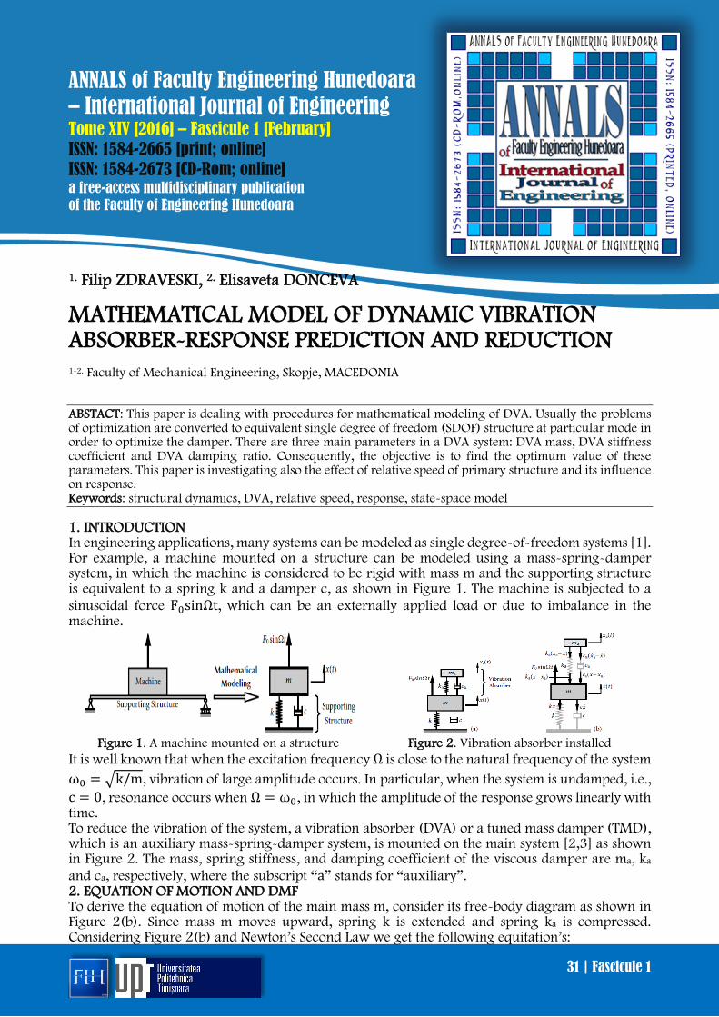
31 | Fascicule 1

ANNALS of Faculty Engineering Hunedoara – International Journal of Engineering Tome XIV [2016] – Fascicule 1 [February] ISSN: 1584-2665 [print; online] ISSN: 1584-2673 [CD-Rom; online] a free-access multidisciplinary publication of the Faculty of Engineering Hunedoara

1. Filip ZDRAVESKI, 2. Elisaveta DONCEVA

MATHEMATICAL MODEL OF DYNAMIC VIBRATION ABSORBER-RESPONSE PREDICTION AND REDUCTION 1-2. Faculty of Mechanical Engineering, Skopje, MACEDONIA ABSTACT: This paper is dealing with procedures for mathematical modeling of DVA. Usually the problems of optimization are converted to equivalent single degree of freedom (SDOF) structure at particular mode in order to optimize the damper. There are three main parameters in a DVA system: DVA mass, DVA stiffness coefficient and DVA damping ratio. Consequently, the objective is to find the optimum value of these parameters. This paper is investigating also the effect of relative speed of primary structure and its influence on response. Keywords: structural dynamics, DVA, relative speed, response, state-space model 1. INTRODUCTION In engineering applications, many systems can be modeled as single degree-of-freedom systems [1]. For example, a machine mounted on a structure can be modeled using a mass-spring-damper system, in which the machine is considered to be rigid with mass m and the supporting structure is equivalent to a spring k and a damper c, as shown in Figure 1. The machine is subjected to a sinusoidal force F0sinΩt, which can be an externally applied load or due to imbalance in the machine.

Figure 1. A machine mounted on a structure Figure 2. Vibration absorber installed

It is well known that when the excitation frequency Ω is close to the natural frequency of the system ω0 = �k/m, vibration of large amplitude occurs. In particular, when the system is undamped, i.e., c = 0, resonance occurs when Ω = ω0, in which the amplitude of the response grows linearly with time. To reduce the vibration of the system, a vibration absorber (DVA) or a tuned mass damper (TMD), which is an auxiliary mass-spring-damper system, is mounted on the main system [2,3] as shown in Figure 2. The mass, spring stiffness, and damping coefficient of the viscous damper are ma, ka and ca, respectively, where the subscript “а” stands for “auxiliary”. 2. EQUATION OF MOTION AND DMF To derive the equation of motion of the main mass m, consider its free-body diagram as shown in Figure 2(b). Since mass m moves upward, spring k is extended and spring ka is compressed. Considering Figure 2(b) and Newton’s Second Law we get the following equitation’s:

ANNALS of Faculty Engineering Hunedoara – International Journal of Engineering

32 | Fascicule 1

mx = ∑ F: mx = −kx − cx − ka(x − xa) − ca(x − xa) + F0sinΩt 1 or

mx + (c + ca)x + (k + ka)x − caxa − kaxa = F0sinΩt 2 Similarly, consider the free-body diagram of mass ma. Since mass ma moves upward a distance xa(t), spring ka is extended. The net extension of spring ka is xa−x. Hence, the spring ka and damper ca exert downward forces ka(xa − x) and ca(xa − x), respectively. Applying Newton’s Second Law gives:

maxa = ∑ F: maxa = −ka(xa − x) − ca(xa − x) 3 or

maxa + caxa + kaxa − cax − kax = 0 4 The Dynamic Magnification Factor (DMF) for mass m is equal to:

DMF =|xP(t)|max

xstatic 5

Adopting the following notations:

ω02 = k

m, c = 2mζω0, r = Ω

ω0 , µ = ma

m, ωa

2 = kama

, ca = 2maζaω0 , ra = ωaω0

6

The Dynamic Magnification Factor becomes: DMF

= ��(ra2 − r2)2 + (2ζar)2

[(1 − r2)(ra2 − r2) − µra2r2 − 4ζaζ r2 ]2 + 4r2[ζa(1 − r2 − µr2) + ζ (ra2 − r2)]2� 7

For the special case when µ = 0, ra = 0, ζa = 0, the Dynamic Magnification Factor reduces to:

DMF =1

�(1 − r2)2 + (2ζr)2 8

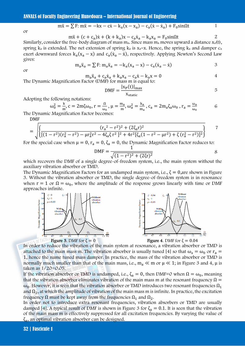
which recovers the DMF of a single degree-of-freedom system, i.e., the main system without the auxiliary vibration absorber or TMD. The Dynamic Magnification Factors for an undamped main system, i.e., ζ = 0,are shown in Figure 3. Without the vibration absorber or TMD, the single degree-of-freedom system is in resonance when r = 1 or Ω = ω0, where the amplitude of the response grows linearly with time or DMF approaches infinite.

Figure 3. DMF for ζ = 0 Figure 4. DMF for ζ = 0.04

In order to reduce the vibration of the main system at resonance, a vibration absorber or TMD is attached to the main mass m. The vibration absorber is usually tuned [4] so that ωа = ω0 or ra =1, hence the name tuned mass damper. In practice, the mass of the vibration absorber or TMD is normally much smaller than that of the main mass, i.e., ma ≪ m or µ ≪ 1; in Figure 3 and 4, μ is taken as 1/20=0.05. If the vibration absorber or TMD is undamped, i.e., ζa = 0, then DMF=0 when Ω = ω0, meaning that the vibration absorber eliminates vibration of the main mass m at the resonant frequency Ω =ω0. However, it is seen that the vibration absorber or TMD introduces two resonant frequencies Ω1 and Ω2, at which the amplitude of vibration of the main mass m is infinite. In practice, the excitation frequency Ω must be kept away from the frequencies Ω1 and Ω2. In order not to introduce extra resonant frequencies, vibration absorbers or TMD are usually damped [4]. A typical result of DMF is shown in Figure 3 for ζa = 0.1. It is seen that the vibration of the main mass m is effectively suppressed for all excitation frequencies. By varying the value of ζa, an optimal vibration absorber can be designed.

ISSN: 1584-2665 [print]; ISSN: 1584-2673 [online]

33 | Fascicule 1

When the main system is also damped, typical results of DMF are shown in Figure 4. Similar conclusions can also be drawn. 3. MATHEMATICAL MODEL OF DYNAMIC VIBRATION ABSORBER WITH MATLAB & SIMULINK Governing equitation’s of motion for the system on Figure 2 can be written as:

mx + (c + ca)x + (k + ka)x − caxa − kaxa = F0sinΩt 9 maxa + caxa + kaxa − cax − kax = 0 10

or in matrix for:

�m 00 ma

� � xxa� + �(c + ca) −ca

−ca ca� � x

xa� + �

(k + ka) −ka−ka ka

� �x

xa� = �10� F0sinΩt 11

Hence MX + CX + KX = I ∙ F0sinΩt 12

In the following step equitation of motion is re-written in State Space system [5]: X = [−M−1K]X + [−M−1C]X + [−M−1I] ∙ F0sinΩt 13 X = [0]X + [1]X + [0] ∙ F0sinΩt 14

or in matrix form:

�XX� = � 0 1 0

0 1−M−1K −M−1C

� �XX� + � 0−M−1I� ∙ F0sinΩt 15

Hence X = A ∙ X + B ∙ u 16

Second equitation of the system is: X = C ∙ X + D ∙ u 17

where

C = �1 ⋯ 0⋮ ⋱ ⋮0 ⋯ 1

� and D = �0 ⋯ 0⋮ ⋱ ⋮0 ⋯ 0

� 18

Above equitation’s conclude the final State-Space form: X = A ∙ X + B ∙ u 19 X = C ∙ X + D ∙ u 20

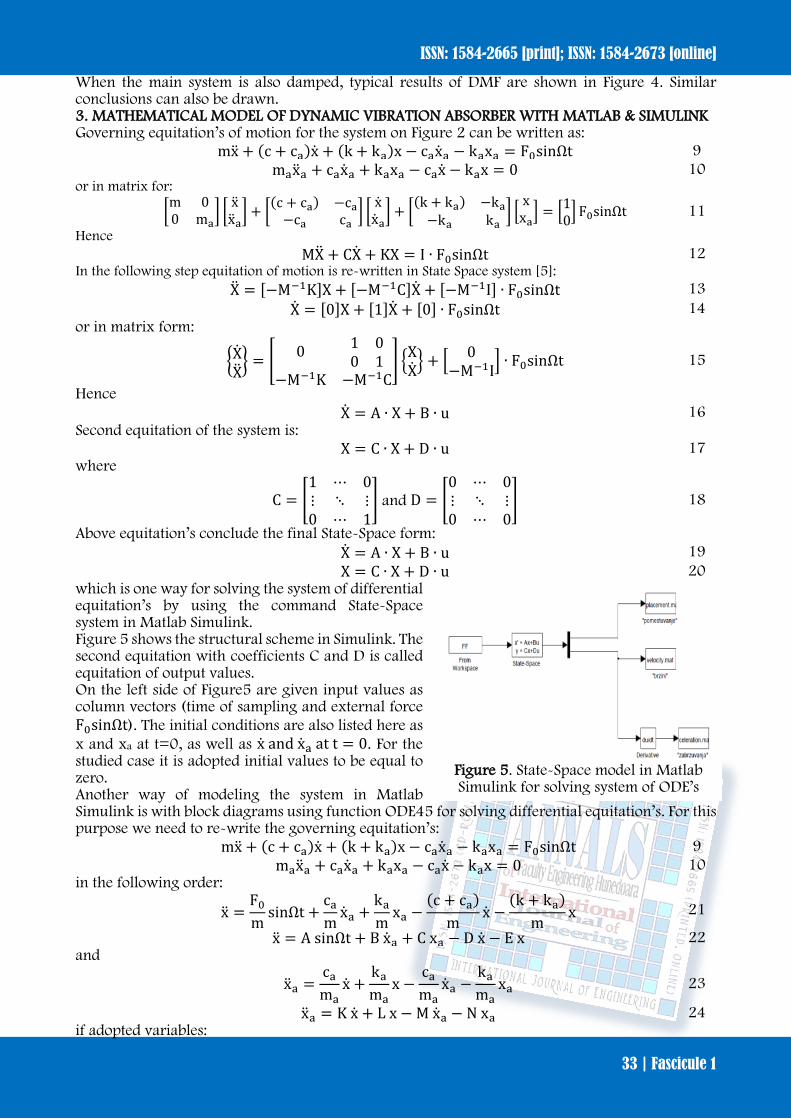
which is one way for solving the system of differential equitation’s by using the command State-Space system in Matlab Simulink. Figure 5 shows the structural scheme in Simulink. The second equitation with coefficients C and D is called equitation of output values. On the left side of Figure5 are given input values as column vectors (time of sampling and external force F0sinΩt). The initial conditions are also listed here as x and xa at t=0, as well as x and xa at t = 0. For the studied case it is adopted initial values to be equal to zero. Another way of modeling the system in Matlab Simulink is with block diagrams using function ODE45 for solving differential equitation’s. For this purpose we need to re-write the governing equitation’s:

mx + (c + ca)x + (k + ka)x − caxa − kaxa = F0sinΩt 9 maxa + caxa + kaxa − cax − kax = 0 10

in the following order:

x =F0m

sinΩt +cam

xa +kam

xa −(c + ca)

mx −

(k + ka)m

x 21

x = A sinΩt + B xa + C xa − D x − E x 22 and

xa =cama

x +kama

x −cama

xa −kama

xa 23

xa = K x + L x − M xa − N xa 24 if adopted variables:

Figure 5. State-Space model in Matlab Simulink for solving system of ODE’s

ANNALS of Faculty Engineering Hunedoara – International Journal of Engineering

34 | Fascicule 1

ω02 = k

m, c = 2mζω0, r = Ω

ω0 , µ = ma

m, ωa

2 = kama

, ca = 2maζaω0, ra = ωaω0

25 the coefficients A, B, C, D, E, K, L, M, N become:

B = 2µζaω0, C = µωa2, D = 2ω0(ζ + µζa), E = ω0

2 + µωa2, K = M = 2ζaω0, L = N = ωa

2 26 Following equitation’s:

x = A sinΩt + B xa + C xa − D x − E x 27 xa = K x + L x − M xa − N xa 28

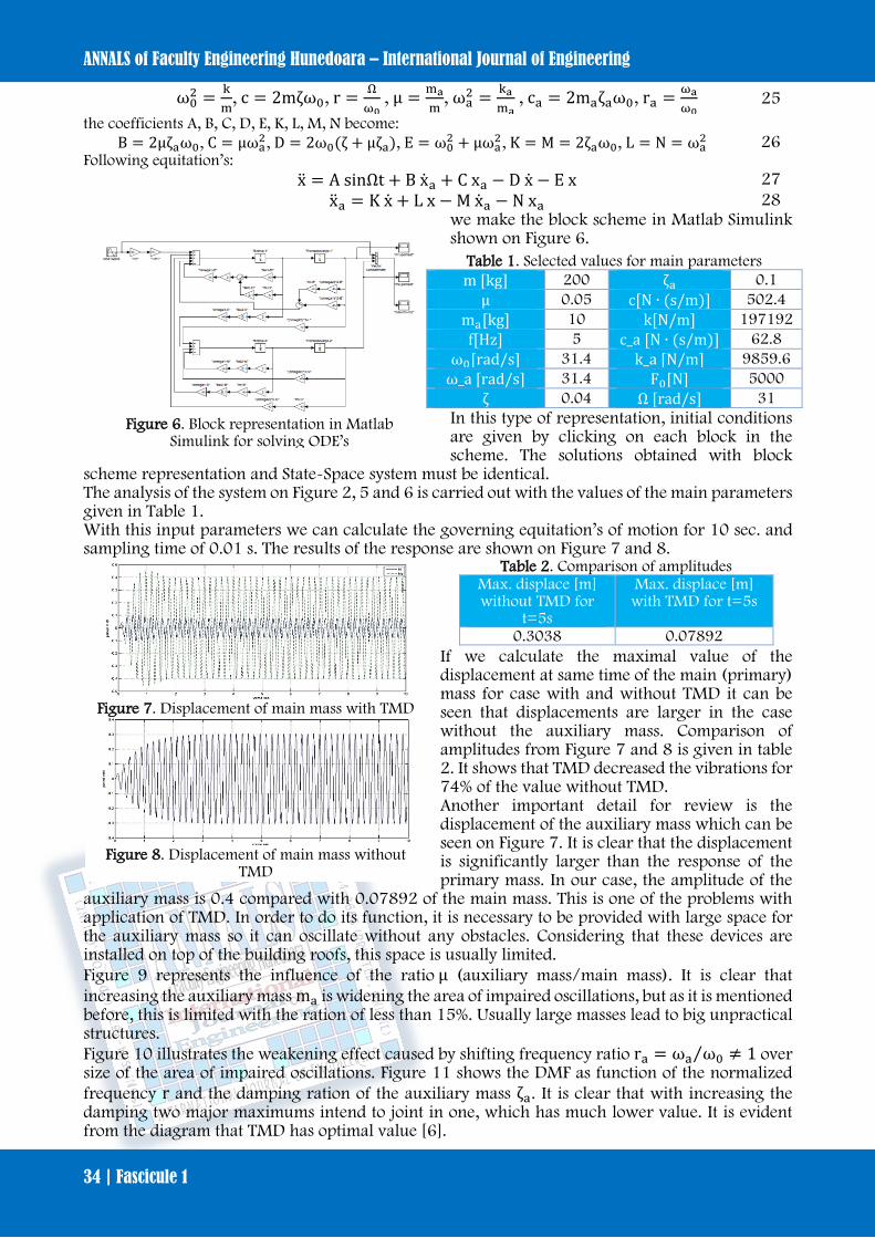
we make the block scheme in Matlab Simulink shown on Figure 6.

In this type of representation, initial conditions are given by clicking on each block in the scheme. The solutions obtained with block

scheme representation and State-Space system must be identical. The analysis of the system on Figure 2, 5 and 6 is carried out with the values of the main parameters given in Table 1. With this input parameters we can calculate the governing equitation’s of motion for 10 sec. and sampling time of 0.01 s. The results of the response are shown on Figure 7 and 8.

Table 2. Comparison of amplitudes Max. displace [m] without TMD for

t=5s

Max. displace [m] with TMD for t=5s

0.3038 0.07892

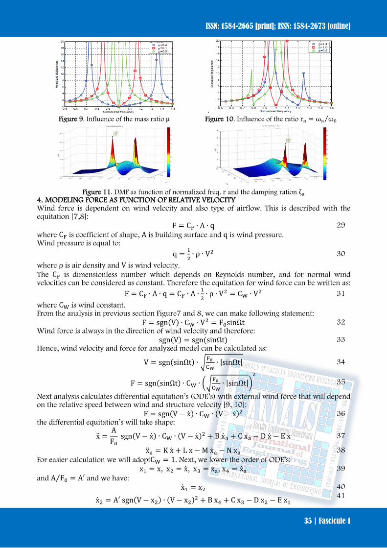
If we calculate the maximal value of the displacement at same time of the main (primary) mass for case with and without TMD it can be seen that displacements are larger in the case without the auxiliary mass. Comparison of amplitudes from Figure 7 and 8 is given in table 2. It shows that TMD decreased the vibrations for 74% of the value without TMD. Another important detail for review is the displacement of the auxiliary mass which can be seen on Figure 7. It is clear that the displacement is significantly larger than the response of the primary mass. In our case, the amplitude of the

auxiliary mass is 0.4 compared with 0.07892 of the main mass. This is one of the problems with application of TMD. In order to do its function, it is necessary to be provided with large space for the auxiliary mass so it can oscillate without any obstacles. Considering that these devices are installed on top of the building roofs, this space is usually limited. Figure 9 represents the influence of the ratio µ (auxiliary mass/main mass). It is clear that increasing the auxiliary mass ma is widening the area of impaired oscillations, but as it is mentioned before, this is limited with the ration of less than 15%. Usually large masses lead to big unpractical structures. Figure 10 illustrates the weakening effect caused by shifting frequency ratio ra = ωa ω0⁄ ≠ 1 over size of the area of impaired oscillations. Figure 11 shows the DMF as function of the normalized frequency r and the damping ration of the auxiliary mass ζa. It is clear that with increasing the damping two major maximums intend to joint in one, which has much lower value. It is evident from the diagram that TMD has optimal value [6].

Figure 6. Block representation in Matlab

Simulink for solving ODE’s

Table 1. Selected values for main parameters m [kg] 200 ζa 0.1 µ 0.05 c[N ∙ (s/m)] 502.4

ma[kg] 10 k[N/m] 197192 f[Hz] 5 c_a [N ∙ (s/m)] 62.8

ω0[rad/s] 31.4 k_a [N/m] 9859.6 ω_a [rad/s] 31.4 F0[N] 5000

ζ 0.04 Ω [rad/s] 31

Figure 7. Displacement of main mass with TMD

Figure 8. Displacement of main mass without

TMD

ISSN: 1584-2665 [print]; ISSN: 1584-2673 [online]

35 | Fascicule 1

. Figure 9. Influence of the mass ratio µ Figure 10. Influence of the ratio ra = ωa ω0⁄

Figure 11. DMF as function of normalized freq. r and the damping ration ζa

4. MODELING FORCE AS FUNCTION OF RELATIVE VELOCITY Wind force is dependent on wind velocity and also type of airflow. This is described with the equitation [7,8]:

F = CF ∙ A ∙ q 29 where CF is coefficient of shape, A is building surface and q is wind pressure. Wind pressure is equal to:

q = 12∙ ρ ∙ V2 30

where ρ is air density and V is wind velocity. The CF is dimensionless number which depends on Reynolds number, and for normal wind velocities can be considered as constant. Therefore the equitation for wind force can be written as:

F = CF ∙ A ∙ q = CF ∙ A ∙ 12∙ ρ ∙ V2 = CW ∙ V2 31

where CW is wind constant. From the analysis in previous section Figure7 and 8, we can make following statement:

F = sgn(V) ∙ CW ∙ V2 = F0sinΩt 32 Wind force is always in the direction of wind velocity and therefore:

sgn(V) = sgn(sinΩt) 33 Hence, wind velocity and force for analyzed model can be calculated as:

V = sgn(sinΩt) ∙ �F0 CW

∙ |sinΩt| 34

F = sgn(sinΩt) ∙ CW ∙ ��F0 CW

∙ |sinΩt|�2

35

Next analysis calculates differential equitation’s (ODE’s) with external wind force that will depend on the relative speed between wind and structure velocity [9, 10]:

F = sgn(V − x) ∙ CW ∙ (V − x)2 36 the differential equitation’s will take shape:

x =AF0

sgn(V − x) ∙ CW ∙ (V − x)2 + B xa + C xa − D x − E x 37

xa = K x + L x − M xa − N xa 38 For easier calculation we will adoptCW = 1. Next, we lower the order of ODE’s:

x1 = x, x2 = x, x3 = xa, x4 = xa 39 and A F0 = A′⁄ and we have:

x1 = x2 40

x2 = A′ sgn(V − x2) ∙ (V − x2)2 + B x4 + C x3 − D x2 − E x1 41

ANNALS of Faculty Engineering Hunedoara – International Journal of Engineering

36 | Fascicule 1

x3 = x4 42 x4 = K x2 + L x1 − M x4 − N x3 43

Using ODE45 (an explicit Runge-Kutta method) in Matlab for solving non-stiff differential equations, we obtain solution for the system above. The results are presented graphically with Figure 12.

Figure 12. Comparison between calculation with and without relative speed included

The results show general trend for smaller amplitudes of displacement of the primary and secondary mass when relative speed is included (Table 3). 5. CONCLUSION This paper is analyzing the mathematical approach for modeling dynamic vibration absorber with s.d.o.f. and m.d.o.f. mass. The paper presents the technique for modeling the differential equitation’s with state-space form and block diagrams using Matlab Simulink. Also, it shows how the relative speed affects the primary mass response under external excitation. It can be concluded that when the primary mass vibrates with frequency close to the natural frequency and it is without TMD the relative speed is causing smaller amplitudes of oscillations. If TMD is installed, the relative speed is not affecting the response of the primary mass and the difference between the amplitudes of oscillations is insignificant. If relative speed is included, the response of primary mass is smaller than the case without it. Note This paper is based on the paper presented at The 12th International Conference on Accomplishments in Electrical and Mechanical Engineering and Information Technology – DEMI 2015, organized by the University of Banja Luka, Faculty of Mechanical Engineering and Faculty of Electrical Engineering, in Banja Luka, BOSNIA & HERZEGOVINA (29th – 30th of May, 2015), referred here as[11]. References [1] Clough,W. R., J.Penzien, Dynamics of Structures, 2rd ed. McGraw-Hill, 1993. Ch. 9-12. [2] Anil K. Chopra, Dynamics of Structures. 4rd ed. Prentice Hall, 2011. Ch. 1-3, 5-7 [3] T. K. Datta, Seismic Analysis of Structures. 1rd ed. John Wiley and Sons, 2010. Ch. 3 and 9 [4] I.Takewaki, Critical Excitation Methods in Earthquake Engineering, 1rd Elsevier Science, 2007. Ch. 5 [5] Aly, A. M., Zasso, A., Resta, F. „Proposed Configuration for the Use of Smart Dampers with Bracings in

Tall Buildings‟. Hindawi Publishing Corporation, Smart Materials Research.2012.Vol.2012. Article ID 251543

[6] Lewandowski, R., Grzymislawska, J. „Dynamic analysis of structure with multiple tuned mass dampers”. Journal of Civil Engineering and Management. 2009. Iss.1. Vol.15. 77-86

[7] Eurocode 1, „Eurocode 1: Actions on structures — General actions — Part 1-4: Wind actions‟. prEN 1991-1-4: European Standard, 2004.

[8] Simiu, Emil, Robert H. Scanlan. Wind effects on structures, Fundamentals and Application to Design. 3rd ed.John Wiley and Sons, 1996. Ch.5

[9] Dyrbye, Claës, S. O. Hansen, Wind Loads on Structures, 1rd ed.John Wiley and Sons, 1997. Ch. 4 and 5 [10] Chen, Shu-Xun. „A More Precise Computation of Along Wind Dynamic Response Analysis for Tall

Buildings Built in Urban Areas‟. Scientific Research Publishing, Journal of Engineering.2010.vol. 2, no.4. 290-2

[11] Filip Zdraveski, Elisaveta Donceva, Mathematical model of dynamic vibration absorber-response prediction and reduction, The 12th International Conference on Accomplishments in Electrical and Mechanical Engineering and Information Technology – DEMI 2015, Banja Luka, BOSNIA & HERZEGOVINA, 459-464

Table 3. Comparison of amplitudes Amplitude of primary mass

for t=5s [m] without TMD (relative speed

included)

without TMD (relative speed not included)

0.25 0.3038 with TMD

(relative speed included)

with TMD (relative speed not included)

0.07467 0.07929