Probing the Circumgalactic Medium at High-Redshift … · Probing the Circumgalactic Medium at...
23
arXiv:1309.6768v2 [astro-ph.CO] 20 Mar 2014 Mon. Not. R. Astron. Soc. 000, 1–19 (x) Printed 21 March 2014 (MN L A T E X style file v2.2) Probing the Circumgalactic Medium at High-Redshift Using Composite BOSS Spectra of Strong Lyman-α Forest Absorbers Matthew M. Pieri 1,2 ⋆ , Michael J. Mortonson 3,8 , Stephan Frank 4 , Neil Crighton 5,6 , David H. Weinberg 4 , Khee-Gan Lee 6 , Pasquier Noterdaeme 7 , Stephen Bailey 8 , Nicolas Busca 9 , Jian Ge 10 , David Kirkby 11 , Britt Lundgren 12 , Smita Mathur 4 , Isabelle Paris 13 , Nathalie Palanque-Delabrouille 7 , Patrick Petitjean 7 , James Rich 14 , Nicholas P. Ross 8 , Donald P. Schneider 15 and Donald G. York 16 1 Institute of Cosmology & Gravitation, University of Portsmouth, Dennis Sciama Building, Portsmouth PO1 3FX, UK 2 CASA, Department of Astrophysical and Planetary Sciences, University of Colorado, 389-UCB, Boulder, CO, USA 80309 3 Space Sciences Lab and Department of Astronomy, University of California, Berkeley, CA 94720, USA 4 Department of Astronomy and CCAPP, Ohio State University, Columbus, OH 43210, USA 5 Centre for Astrophysics and Supercomputing, Swinburne University of Technology, PO Box 218, Victoria 3122, Australia 6 Max-Planck-Institut f¨ ur Astronomie, K¨ onigstuhl 17, 69117 Heidelberg, Germany 7 Institut d’Astrophysique de Paris, CNRS-UPMC, UMR 7095, 98bis bd Arago, 75014, Paris, France [email protected] 8 Lawrence Berkeley National Lab, 1 Cyclotron Rd, Berkeley CA, 94720, USA 9 APC, Universit´ e Paris Diderot-Paris 7, CNRS/IN2P3, CEA, Observatoire de Paris, 10, rueA. Domon & L. Duquet, Paris, France 10 Astronomy Department, University of Florida, 211 Bryant Space Science Center, Gainesville, FL 32611-2055 11 Department of Physics and Astronomy, University of California, Irvine, 4129 Frederick Reines Hall, Irvine, CA 92697-4575, USA 12 Department of Astronomy, University of Wisconsin, 475 North Charter Street, Madison, WI 53706, USA 13 Departamento de Astronom´ ıa, Universidad de Chile, Casilla 36-D, Santiago, Chile 14 CEA, Centre de Saclay, IRFU, F-91191 Gif-sur-Yvette, France 15 Department of Astronomy and Astrophysics, and Institute for Gravitation and the Cosmos, The Pennsylvania State University, University Park, PA 16802 16 Department of Astronomy and Astrophysics and the Enrico Fermi Institute, The University of Chicago, 5640 South Ellis Avenue, Chicago, Illinois, 60615, USA Accepted xxxx ABSTRACT We present composite spectra constructed from a sample of 242,150 Lyman-α (Lyα ) forest absorbers at redshifts 2.4 < z < 3.1 identified in quasar spectra from the Baryon Oscil- lation Spectroscopic Survey (BOSS) as part of Data Release 9 of the Sloan Digital Sky Survey III. We select forest absorbers by their flux in bins 138 km s −1 wide (approximately the size of the BOSS resolution element). We split these absorbers into five samples spanning the range of flux −0.05 F < 0.45. Tests on a smaller set of high-resolution spectra show that our three strongest absorption samples would probe circumgalactic regions (projected separation < 300 proper kpc and |∆v| < 300 km s −1 ) in about 60% of cases for very high signal-to-noise ratio. Within this subset, weakening Lyα absorption is associated with decreasing purity of circum- galactic selection once BOSS noise is included. Our weaker two Lyα absorption samples are dominated by the intergalactic medium. We present composite spectra of these samples and a catalogue of measured absorption features from H I and 13 metal ionization species, all of which we make available to the community. We compare measurements of seven Lyman series transitions in our composite spectra to single line models and obtain further constraints from their associated excess Lyman limit opacity. This analysis provides results consistent with column densities over the range 14.4 log(N HI ) 16.45. We compare our measurements of metal absorption to a variety of simple single-line, single-phase models for a preliminary interpretation. Our results imply clumping on scales down to ∼ 30 pc and near-solar metallicities in the circumgalactic samples, while high-ionization metal absorption consistent with typical IGM densities and metallicities is visible in all samples. Key words: intergalactic medium, quasars: absorption lines, galaxies: formation, galaxies: evolution, galaxies: high-redshift c x RAS
Transcript of Probing the Circumgalactic Medium at High-Redshift … · Probing the Circumgalactic Medium at...
arX
iv:1
309.
6768
v2 [
astr
o-ph
.CO
] 20
Mar
201
4Mon. Not. R. Astron. Soc.000, 1–19 (x) Printed 21 March 2014 (MN LATEX style file v2.2)
Probing the Circumgalactic Medium at High-Redshift UsingComposite BOSS Spectra of Strong Lyman-α Forest Absorbers
Matthew M. Pieri1,2⋆, Michael J. Mortonson3,8, Stephan Frank4, Neil Crighton5,6,David H. Weinberg4, Khee-Gan Lee6, Pasquier Noterdaeme7, Stephen Bailey8,Nicolas Busca9, Jian Ge10, David Kirkby11, Britt Lundgren12, Smita Mathur4,Isabelle Paris13, Nathalie Palanque-Delabrouille7, Patrick Petitjean7, James Rich14,Nicholas P. Ross8, Donald P. Schneider15 and Donald G. York161Institute of Cosmology & Gravitation, University of Portsmouth, Dennis Sciama Building, Portsmouth PO1 3FX, UK2CASA, Department of Astrophysical and Planetary Sciences,University of Colorado, 389-UCB, Boulder, CO, USA 803093Space Sciences Lab and Department of Astronomy, Universityof California, Berkeley, CA 94720, USA4Department of Astronomy and CCAPP, Ohio State University, Columbus, OH 43210, USA5Centre for Astrophysics and Supercomputing, Swinburne University of Technology, PO Box 218, Victoria 3122, Australia6Max-Planck-Institut fur Astronomie, Konigstuhl 17, 69117 Heidelberg, Germany7Institut d’Astrophysique de Paris, CNRS-UPMC, UMR 7095, 98bis bd Arago, 75014, Paris, France [email protected] Berkeley National Lab, 1 Cyclotron Rd, Berkeley CA, 94720, USA9APC, Universite Paris Diderot-Paris 7, CNRS/IN2P3, CEA, Observatoire de Paris, 10, rueA. Domon & L. Duquet, Paris, France10Astronomy Department, University of Florida, 211 Bryant Space Science Center, Gainesville, FL 32611-205511Department of Physics and Astronomy, University of California, Irvine, 4129 Frederick Reines Hall, Irvine, CA 92697-4575, USA12Department of Astronomy, University of Wisconsin, 475 North Charter Street, Madison, WI 53706, USA13Departamento de Astronomıa, Universidad de Chile, Casilla 36-D, Santiago, Chile14CEA, Centre de Saclay, IRFU, F-91191 Gif-sur-Yvette, France15Department of Astronomy and Astrophysics, and Institute for Gravitation and the Cosmos, The Pennsylvania State University, University Park, PA 1680216Department of Astronomy and Astrophysics and the Enrico Fermi Institute, The University of Chicago, 5640 South Ellis Avenue, Chicago, Illinois, 60615, USA
Accepted xxxx
ABSTRACT
We present composite spectra constructed from a sample of 242,150 Lyman-α (Lyα)forest absorbers at redshifts 2.4< z< 3.1 identified in quasar spectra from the Baryon Oscil-lation Spectroscopic Survey (BOSS) as part of Data Release 9of the Sloan Digital Sky SurveyIII. We select forest absorbers by their flux in bins 138 kms−1 wide (approximately the size ofthe BOSS resolution element). We split these absorbers intofive samples spanning the rangeof flux −0.056 F < 0.45. Tests on a smaller set of high-resolution spectra show that our threestrongest absorption samples would probe circumgalactic regions (projected separation< 300proper kpc and|∆v|< 300 kms−1) in about 60% of cases for very high signal-to-noise ratio.Within this subset, weakening Lyα absorption is associated with decreasing purity of circum-galactic selection once BOSS noise is included. Our weaker two Lyα absorption samples aredominated by the intergalactic medium.
We present composite spectra of these samples and a catalogue of measured absorptionfeatures from HI and 13 metal ionization species, all of which we make available to thecommunity. We compare measurements of seven Lyman series transitions in our compositespectra to single line models and obtain further constraints from their associated excess Lymanlimit opacity. This analysis provides results consistent with column densities over the range14.4 . log(NHI) . 16.45. We compare our measurements of metal absorption to a varietyof simple single-line, single-phase models for a preliminary interpretation. Our results implyclumping on scales down to∼30 pc and near-solar metallicities in the circumgalactic samples,while high-ionization metal absorption consistent with typical IGM densities and metallicitiesis visible in all samples.
Key words: intergalactic medium, quasars: absorption lines, galaxies: formation, galaxies:evolution, galaxies: high-redshift
c© x RAS
2 Pieri M. M. et al.
1 INTRODUCTION
Since the birth of the first stars, the formation and evolution ofgalaxies has been intertwined with the evolution of intergalacticand circumgalactic media. These reservoirs of gas feed starforma-tion and galaxy assembly, but also reflect the history of starforma-tion by virtue of the presence and properties of heavy elements.Knowledge of the degree of enrichment by metals in the inter-galactic medium (IGM) and circumgalactic medium (CGM) allowsexploration of the energetics of mechanical outflows from galax-ies (e.g. Mac Low & Ferrara 1999; Scannapieco, Ferrara & Madau2002; Pieri, Martel & Grenon 2007; Pinsonneault, Martel & Pieri2010). These outflows are a key component in our understand-ing of galaxy formation as they have the potential to heat andeject gas from dark matter halos, suppressing star formation, orincrease the cooling rate by depositing metals, promoting starformation (e.g. Aguirre et al. 2001; Oppenheimer & Dave 2006;Schaye et al. 2010; Barai et al. 2013). The pattern of elementalabundances present may also reveal the stellar populationsthat giverise to them. The abundance of individual ionization species ofthese elements allows investigation of the extragalactic UV back-ground (due to the impact of photoionization), and the density andtemperature of the gas (due to collisional ionization and recombina-tion). A large number of metal species are required to measure all ofthese effects and break degeneracies between them (Aguirreet al.2008; Pieri et al. 2010b). In this paper, we apply a novel analysistechnique; we stack quasar spectra on the rest-frame locations ofLyα absorbers (Pieri et al. 2010b, P10 hereafter) in the enormousspectral database of the Baryon Oscillation SpectroscopicSurvey(BOSS, Dawson et al. 2013). This affords the derivation of con-straints on the metal enrichment and ionization state of intergalacticand circumgalactic gas.
The distribution of gas on large scales and its metal propertiesmay be probed by measuring intervening absorbers along the lineof sight to bright background quasars. The aptly named Lyman-αforest is a crowded distribution of absorption lines associated withtrace amounts of neutral hydrogen (or HI) in this largely photoion-ized medium (Gunn & Peterson 1965; Lynds 1971). It provides usdetailed information on the density of structure over a significantrange of redshifts for each quasar spectrum. Most of the Lyman-α(Lyα) forest is associated with moderate overdensities (ρ/ρ ∼ 1–10) and traces filamentary structure on large scales, but some strongforest absorbers along with Lyman limit systems and dampedLyman-α systems (DLAs) are thought to be associated with galax-ies and the circumgalactic medium (e.g. Faucher-Giguere &Keres2011; Fumagalli et al. 2011).
These spectra also allow measurement of a variety of metalspecies in principle, but in practise only a limited numberare detectable in the Lyα forest. Three-times-ionized carbon orC IV (e.g. Meyer & York 1987; Cowie et al. 1995; Schaye et al.2003; Pieri, Schaye & Aguirre 2006) and five-times-ionized oxy-gen or OVI (e.g. Schaye et al. 2000; Pieri & Haehnelt 2004;Simcoe, Sargent & Rauch 2004; Pieri et al. 2010a) are particularlywell-observed. Many other weak lines are challenging to detect, butprogress has been made towards this goal (P10) by stacking Lyαforest lines in Sloan Digital Sky Survey II Data Release 5 (SDSS-II DR5; York et al. 2000; Adelman-McCarthy et al. 2007) quasarspectra.
Associations between galaxies and intervening absorbers areeasier to establish at low-redshifts where the galaxies areread-ily identified (e.g. Tumlinson et al. 2011; Lundgren et al. 2012;Stocke et al. 2013; Nielsen et al. 2013). Significant challenges ex-
ist in surveying galaxies at high-redshift (z> 2), particularly sincemuch of this population is expected to be composed of faint,dwarf galaxies (e.g. Pieri & Martel 2007, A. Rahmati et al inprep). Efforts are underway to build large samples of galaxies us-ing the Lyman break technique (known as ‘Lyman break galax-ies’ or LBGs). Samples such as the Keck Baryon Structure Survey(KBSS, Steidel et al. 2010; Rudie et al. 2012; Rakic et al. 2012)and the VLT LBG survey (Crighton et al. 2011) are being usedto study the interaction of galaxies and the IGM/CGM, but thesesurveys have yet to show many weaker lines in optically thin gas.Progress has also been made by using observations of galaxies toexplore the properties of their own circumgalactic regions(Martin2005; Steidel et al. 2010), but ambiguities exist between small-scale galactic effects and larger scale circumgalactic absorption.
We present an alternative approach using absorbers as aproxy for galactic and circumgalactic regions in order to con-struct a much larger sample and so have greater sensitivity toweaker metal transitions. This approach is not without precedent;Pieri, Schaye & Aguirre (2006) used strong CIV lines as a proxyfor galaxy locations motivated by observations of LBGs and nearbyquasars (Adelberger et al. 2003). This approach was primarily usedto investigate the existence of metals far from known galaxies.Lehner et al. (2013) use partial Lyman limit systems and Lymanlimit systems as a proxy for galaxies atz . 1. In addition P10stacked strong, blended Lyα forest lines in the SDSS-II DR5 sam-ple and found indications of circumgalactic conditions in the resul-tant composite spectra.
We return to the analysis of P10 with methodological modifi-cations, a larger data set from Data Release 9 (Ahn et al. 2012) ofSDSS-III (Eisenstein et al. 2011), more extensive results,and in-vestigations of our selection function using simulated spectra andhigh-resolution spectra with LBG proximity from the VLT LBGsurvey. We present a catalogue of composite spectra for varyingLyα absorber strength, each with measurements of seven Lymanseries lines, Lyman limit opacity, and 26 metal transitionsfrom 7elements and 13 ionization species. We also publish our compositespectra online to enable alternative measurements of the absorptionprofiles. We perform a preliminary interpretation of our measure-ments including constraints on gas metallicity and absorber sizes.In future work, we will carry out direct comparisons to the predic-tions of cosmological hydrodynamic simulations.
This paper is structured as follows. In Section 2, we describethe data used in this analysis. In Section 3, we describe our selec-tion of Lyα absorbers and investigate the kind of systems and en-vironments it picks out, appealing to both simulations and the VLTLBG analysis. Section 4 sets out the method we used to producecomposite spectra of these absorbers. In Section 5, we describe ourresults including characterisation of HI absorption, measurementsof metals, and comparison to simple models. Section 6 provides adiscussion of our results and it is followed by a summary.
We assume a solar pattern of elemental abundances taken fromAnders & Grevesse (1989) for our interpretation. There are anum-ber of alternative choices available, but the differences are small onthe scale of the effects discussed here.
2 DATA
The Baryon Oscillation Spectroscopic Survey is one of four spec-troscopic surveys that make up SDSS-III (Eisenstein et al. 2011),all conducted from the 2.5-meter Sloan telescope (Gunn et al.2006) at Apache Point Observatory. The BOSS instrument
c© x RAS, MNRAS000, 1–19
Probing the Circumgalactic Medium at High-Redshift3
(Smee et al. 2013) consists of two double spectrographs eachwitha blue channel and a red channel. We use the SDSS-III Data Re-lease 9 (Ahn et al. 2012) high-redshift quasar sample, selected us-ing the techniques and data outlined in Ross et al. (2012) (seealso Bovy et al. 2011). The sample of high-redshift quasars wascompiled by visual inspection of quasar candidates as outlined inParis et al. (2012).
The resolution of these spectra varies overR≈ 1650 toR≈2500 and is broadly lower (higher) at the low (high) wavelengthend of both the blue and red channel of each BOSS spectrograph.In the portion of the spectra we use for selecting Lyα absorbers,it varies over 1650. R. 2150. We assume a constant value ofR=2000 when fitting line properties, and this assumption will leadto small systematic errors in our line widths; however, we donotdraw detailed conclusions from line widths in this paper. The BOSSspectrograph provides coverage over the wavelength range 3450–10400A, although the signal-to-noise ratio (S/N) declines at theblue end, and much of the redward end of the spectra is discardeddue to strong sky lines.
The SDSS spectroscopic pipeline (Bolton et al. 2012) per-forms the basic data reduction and calibration of quasar spectra.For our analysis we make use of several, publicly available,valueadded products from Lee et al. (2013) including principal compo-nent analysis (PCA) continua, a correction of spectral residuals(associated with a small error introduced by imperfect masking ofBalmer lines in spectroscopic standard stars used for flux calibra-tion) and zero-velocity calcium H+K absorption lines (likely asso-ciated with the Milky Way halo), a supplementary mask of sky linesin addition to those provided by the SDSS pipeline, and correctionsfor known biases in the pipeline estimated noise. There are 54,468quasars in the Lee et al. (2013) sample with redshifts providing in-tergalactic Lyα forest coverage (zq > 2.15).
In order to arrive at a sample well-suited to the purpose of se-lecting absorbers in a meaningful way, we implement a quality cutdescribed in Section 3, and as a result, only 30,555 of these spectraprovide a portion of the forest in the desired redshift rangeof suf-ficient quality, with a total redshift path of∆z= 3409. This sectionalso explains our decision to rebin our sample by a factor of 2com-pared to the SDSS pipeline, giving 138 kms−1 wide wavelengthbins. DLAs from the Noterdaeme et al. (2012) catalogue were ex-cluded from the analysis. We reject DLAs in order to improve thehomogeneity of our selection of strong, blended Lya forest linesand simplify interpretation (although we note that their omissionhad negligible impact due to their scarcity in the sample). Theircores were masked using the value added flags in Lee et al. (2013).In addition, the wings of these lines were masked where the pro-vided fits indicated a greater than 5% flux decrement. These cutsproduce a sample of 242,150 Lyα forest absorbers in 138 kms−1
wide bins in a renormalised flux range from−0.056 F < 0.45.We use two different methods for renormalising the quasar
continua to probe intervening absorbers, one for our selection ofLyα absorbers to stack and another for creating spectra to stack.PCA continua (Lee, Suzuki & Spergel 2012) are used for the selec-tion of absorbers to stack, but these continua are limited to1030-1600A in the quasar rest-frame. This approach is adequate for Lyαselection since we only stack Lyα absorbers that are free from con-tamination by higher order Lyman lines.
We perform an absorption-rejecting cubic spline fit to estimatethe continuum level over the full spectral range. The PCA continuaprovide more robust absolute measurements of Lyα absorbers, butour spline fits are of sufficient quality for the stacking of spectra,where it is only necessary that they be smooth with respect tothe
width of absorbers and that they remove the bulk of the quasarproperties. Any remaining quasar properties will contribute onlyweak stochastic error in our composite spectra due to our pseudo-continuum fitting of stacked spectra (see Section 4).
We fit a cubic spline to nodes measured as the median flux in20A wide chunks. We discard any blueward band with a 100-pixel(6900 kms−1) boxcar smoothed S/N< 1 as our absorption rejec-tion procedure performs poorly where the noise is greater than thesignal. We iteratively refine the median flux of these nodes byre-jecting negative deviations from the spline greater than the spectralerror estimate in the forest and twice the spectral error outside theforest. We do not fit within±15A of Lyα and CIV transitions inthe quasar rest-frame since these emission line centres aretoo sharpto produce a good fit. We then discard points within±20A of thesefeatures, an extra 5A padding, because spline fits can produce un-stable results when presented with sharp edges.
3 LYMAN α ABSORBER SELECTION
Given the sensitivity of stacking analyses to the selectionof objects,we have developed our selection with the aid of simulated spectrawhich are a close reproduction of those present in the BOSS Lyαsurvey. These simulations are described in detail in our future pa-per (M. Mortonson et al. in prep), but we will briefly summarisethem below (Section 3.1). Our selection function is imposedon uspredominantly by the resolution of the data. Our goal is to explorethe statistical properties of systems selected by this procedure.
We select Lyα absorbers in the redshift range 2.4< z< 3.1.This choice is motivated by our desire to obtain high qualityspec-tral coverage of the Lyman limit at the blue limit and MgII at thered limit in stacked spectra. The spectral resolution in oursampleequates to a full width half maximum (FWHM) of 2–2.6 pixels(138–179 kms−1) in the standard SDSS spectral wavelength solu-tion. Because of the critical impact of S/N on our absorber selec-tion, we rebin the spectra by a factor of 2 before selection toreducenoise, with only minimal loss of resolving power. This provides usa wavelength bin size of 138 kms−1, and has the additional benefitof precluding double-counting of absorption from the same resolu-tion element.
We use only the flux in these rescaled bins (with a quality cutdescribed below) to select systems for stacking. We presentfivesamples of Lyα absorbers for stacking, with(0.1n−0.05) 6 F <(0.1n+0.05), wheren = 0,1, . . . ,4. Our simulations described inSection 3.2 indicate that this value of∆F is a good reflection of ourability to produce distinct samples when an appropriate quality cutis used. In order of increasing flux (and hence decreasing absorp-tion) our samples include 11441, 25128, 42034, 65045 and 98502absorbers.
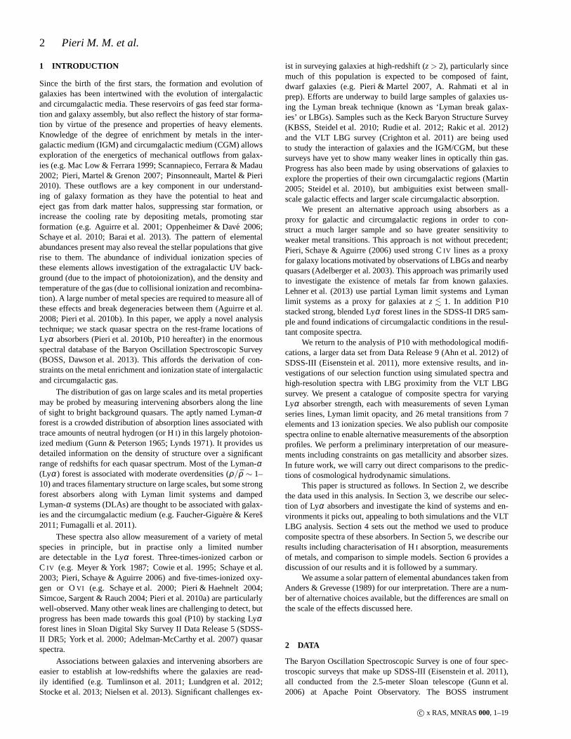
At BOSS resolution with 138 kms−1 bins, a Lyα forest lineof typical width with no damping wings does not reach saturation,regardless of its column density. The distribution of Doppler pa-rameters in the Lyα forest is well characterised by a Gaussian withmedianb ≈ 30 kms−1 and σ = 10 kms−1 that is cropped belowb =15–20 kms−1 (e.g Hu et al. 1995; Rudie et al. 2012). As Fig-ure 1 shows, only single lines with logNHI & 18 or unusually highDoppler parameters (> 40 kms−1) reach a minimum flux belowF = 0.15. Therefore, fluxes below this limit generally arise fromblends of lines, and even at higher fluxes blends of weak linesmaydominate by number over isolated strong lines. The 2-pixel rebin-ning increases the degree to which blending affects the selection.We discuss the significance of this selection function further in re-
c© x RAS, MNRAS000, 1–19
4 Pieri M. M. et al.
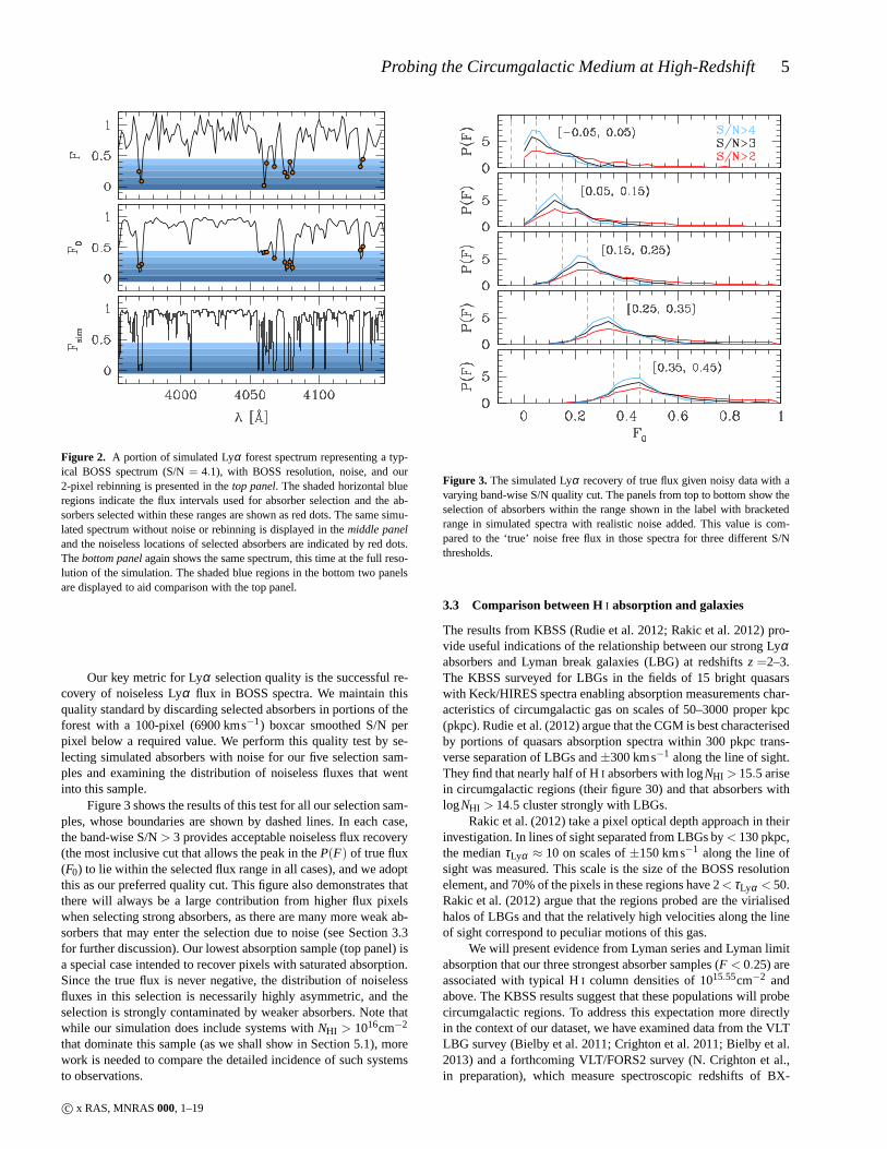
Figure 1. The minimum Lyα forest flux reached in single line models atBOSS resolution in a 138 kms−1 bin.
lation to simulations in Section 3.2 and circumgalactic regions inSection 3.3.
As we show in Section 5, the inferred HI column in our sam-ples are characteristic of saturated lines that don’t generate signifi-cant opacity at the Lyman limit in individual high-resolution spec-tra. This effect makes such systems challenging to identifywith-out appealing to Lyβ observations (Kim et al. 2002), which arethemselves difficult to confidently distinguish from Lyα absorbers.However, our sample successfully probes this regime.
Our sample of absorbers is drawn from wavelengths 1041A <λ < 1185A in the quasar rest-frame. We make this choice to elim-inate the selection of OVI absorbers and absorbers proximate tothe quasar (within 7563 kms−1). We assume that all remaining ab-sorbers arise due to the Lyman-α transition and so are availablefor selection. As we discuss in§5.2 this assumption is not alwaysvalid, but typically the cases where it does fail are distinct fromthe effects we intend to measure, and the breakdowns themselvesprovide useful information about metal interlopers.
3.1 Production of simulated spectra
The simulated Lyα spectra we use to study issues related to ab-sorber selection are generated by computing the transmitted fluxfraction F along random sightlines through an N-body+smoothedparticle hydrodynamic (SPH) simulation in a 100h−1 Mpc boxwith 2×5763 particles (with equal numbers of gas and dark mat-ter particles). The simulation was run with a version of the codeGADGET-2 (Springel 2005) with several modifications describedby Oppenheimer & Dave (2008), including modeling of galacticoutflows with a momentum-driven wind model. The cosmologi-cal parameters assumed for the simulation are consistent with re-sults from the Five-Year Wilkinson Microwave Anisotropy Probe(WMAP5, Hinshaw et al. 2009). For the analysis presented here,we use only thez= 2.5 simulation output.
For each sightline through the simulation volume, we runthe SPECEXBIN code (Oppenheimer & Dave 2006), which com-putes the gas density, temperature, metallicity, and velocity con-tributed by all SPH particles intersecting the line of sight. It utilisesthose quantities to compute the redshift-space optical depth alongthe sightline for Lyα and several metal lines, assuming ionizationequilibrium to determine the ionization fraction for a given densityand temperature. In this paper, we use simulations only to calibrate
Lyα absorber selection, so we only use the Lyα optical depthτLyαfrom SPECEXBIN; simulated spectra that include additionalLy-man series lines and metal lines will be studied in our forthcomingcomparison paper (M. Mortonson et al., in prep.), which willalsodescribe the simulation itself in greater detail.
To produce simulated spectra that match the absorber redshiftdistribution, resolution, and noise properties of the BOSSDR9sample, we use measurements from the Lee et al. (2013) sampleof quasar spectra and value added products. For each high-redshiftquasar in this sample, we divide the observed Lyα forest wave-length range (specifically, 1041A < λ < 1185A in the quasar rest-frame) into segments with length equal to the simulated sightlinesdescribed above, i.e. 100h−1 Mpc. Typically, 3–5 such segmentsare required to cover the Lyα forest for each quasar. For each seg-ment, we randomly draw one of the simulated 100h−1 Mpc sight-lines and shift it by a random offset in the line of sight direc-tion using the periodic boundary conditions of the simulation vol-ume. We multiply allτLyα values along the sightline by a factorτeff(z)/τeff,sim, whereτeff,sim = 0.233 is the effective Lyα opticaldepth measured in thez= 2.5 simulation andτeff(z) is the observedpower-law relation from Faucher-Giguere et al. (2008) evaluated atthe appropriate redshift for Lyα absorption at the observed wave-length. All of the rescaled sightlines are combined into a singleLyα forest spectrum of transmitted fluxFsim = exp(−τLyα ) foreach quasar.
We smooth the resulting spectrumFsim(λ ) to BOSS resolutionby convolving it with a Gaussian with width equal to the actualwavelength-dependent dispersion for the quasar spectrum from theDR9 sample. We then resample the smoothed flux on the SDSSwavelength solution; we designate the smoothed and pixelized (butstill noise-free) flux fractionF0.
Finally, we add simulated noise to the spectrum:F = F0+N.For each pixel, we drawN from a Gaussian with wavelength- andflux-dependent variance
σ2F(λ ) = k(λ )
F0(λ )Cobs(λ )+Sobs(λ )Cobs(λ )2
, (1)
whereCobs(λ ) andSobs(λ ) are the estimated continuum flux andsky background flux, respectively, from the actual quasar spectrumin the Lee et al. (2013) catalog, and at each observed wavelengthλ , k(λ ) is the coefficient that best fits the relation in equation (1) asmeasured in the BOSS DR9 sample of quasar spectra (replacingF0with the observed flux fractionFobs and using the estimated noisevariance forσ2
F ).
3.2 Simulation motivated selection
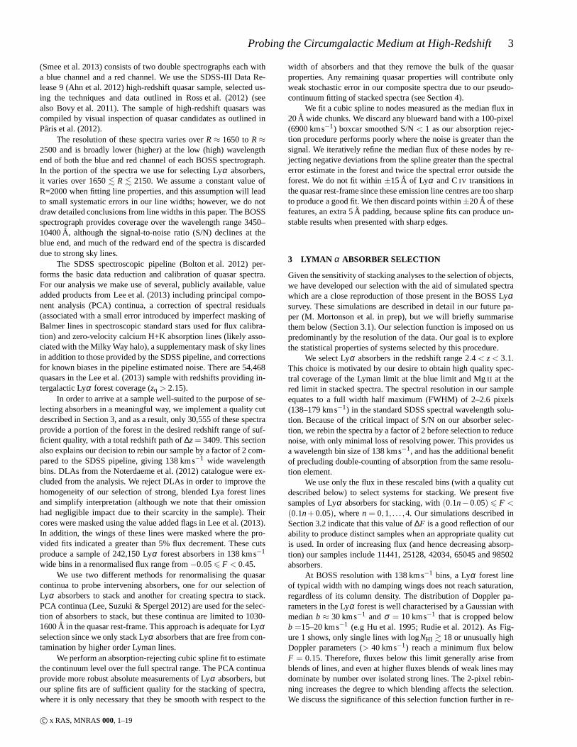
Figure 2 provides an illustration of the typical spectral character-istics that form part of our selection. The bottom panel presents aportion of spectrum with simulation resolution (reproducing datawith fully resolved lines) and no noise. The middle panel showsthe same portion of simulated spectrum with BOSS resolution, our2-pixel rebinning, and no noise. Comparison of these two panelsconfirms that low flux at high-resolution is not sufficient to producelow flux at BOSS resolution; a degree of blending is also required.The top panel displays the same spectrum as the middle panel withthe addition of typical noise in our sample. Note that we treat eachwavelength bin that falls into our target flux range as an absorber.As is clear in this figure, adjacent strongly absorbed wavelengthbins arise from extended structure in velocity space, and not ther-mal wings of lines.
c© x RAS, MNRAS000, 1–19
Probing the Circumgalactic Medium at High-Redshift5
Figure 2. A portion of simulated Lyα forest spectrum representing a typ-ical BOSS spectrum (S/N= 4.1), with BOSS resolution, noise, and our2-pixel rebinning is presented in thetop panel. The shaded horizontal blueregions indicate the flux intervals used for absorber selection and the ab-sorbers selected within these ranges are shown as red dots. The same simu-lated spectrum without noise or rebinning is displayed in the middle paneland the noiseless locations of selected absorbers are indicated by red dots.Thebottom panelagain shows the same spectrum, this time at the full reso-lution of the simulation. The shaded blue regions in the bottom two panelsare displayed to aid comparison with the top panel.
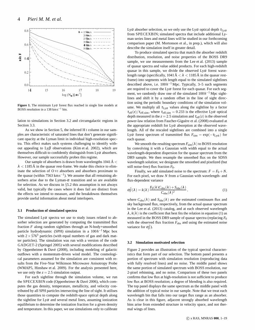
Our key metric for Lyα selection quality is the successful re-covery of noiseless Lyα flux in BOSS spectra. We maintain thisquality standard by discarding selected absorbers in portions of theforest with a 100-pixel (6900 kms−1) boxcar smoothed S/N perpixel below a required value. We perform this quality test byse-lecting simulated absorbers with noise for our five selection sam-ples and examining the distribution of noiseless fluxes thatwentinto this sample.
Figure 3 shows the results of this test for all our selection sam-ples, whose boundaries are shown by dashed lines. In each case,the band-wise S/N> 3 provides acceptable noiseless flux recovery(the most inclusive cut that allows the peak in theP(F) of true flux(F0) to lie within the selected flux range in all cases), and we adoptthis as our preferred quality cut. This figure also demonstrates thatthere will always be a large contribution from higher flux pixelswhen selecting strong absorbers, as there are many more weakab-sorbers that may enter the selection due to noise (see Section 3.3for further discussion). Our lowest absorption sample (toppanel) isa special case intended to recover pixels with saturated absorption.Since the true flux is never negative, the distribution of noiselessfluxes in this selection is necessarily highly asymmetric, and theselection is strongly contaminated by weaker absorbers. Note thatwhile our simulation does include systems withNHI > 1016cm−2
that dominate this sample (as we shall show in Section 5.1), morework is needed to compare the detailed incidence of such systemsto observations.
Figure 3. The simulated Lyα recovery of true flux given noisy data with avarying band-wise S/N quality cut. The panels from top to bottom show theselection of absorbers within the range shown in the label with bracketedrange in simulated spectra with realistic noise added. Thisvalue is com-pared to the ‘true’ noise free flux in those spectra for three different S/Nthresholds.
3.3 Comparison between HI absorption and galaxies
The results from KBSS (Rudie et al. 2012; Rakic et al. 2012) pro-vide useful indications of the relationship between our strong Lyαabsorbers and Lyman break galaxies (LBG) at redshiftsz=2–3.The KBSS surveyed for LBGs in the fields of 15 bright quasarswith Keck/HIRES spectra enabling absorption measurementschar-acteristics of circumgalactic gas on scales of 50–3000 proper kpc(pkpc). Rudie et al. (2012) argue that the CGM is best characterisedby portions of quasars absorption spectra within 300 pkpc trans-verse separation of LBGs and±300 kms−1 along the line of sight.They find that nearly half of HI absorbers with logNHI > 15.5 arisein circumgalactic regions (their figure 30) and that absorbers withlogNHI > 14.5 cluster strongly with LBGs.
Rakic et al. (2012) take a pixel optical depth approach in theirinvestigation. In lines of sight separated from LBGs by< 130 pkpc,the medianτLyα ≈ 10 on scales of±150 kms−1 along the line ofsight was measured. This scale is the size of the BOSS resolutionelement, and 70% of the pixels in these regions have 2< τLyα < 50.Rakic et al. (2012) argue that the regions probed are the virialisedhalos of LBGs and that the relatively high velocities along the lineof sight correspond to peculiar motions of this gas.
We will present evidence from Lyman series and Lyman limitabsorption that our three strongest absorber samples (F < 0.25) areassociated with typical HI column densities of 1015.55cm−2 andabove. The KBSS results suggest that these populations willprobecircumgalactic regions. To address this expectation more directlyin the context of our dataset, we have examined data from the VLTLBG survey (Bielby et al. 2011; Crighton et al. 2011; Bielby et al.2013) and a forthcoming VLT/FORS2 survey (N. Crighton et al.,in preparation), which measure spectroscopic redshifts ofBX-
c© x RAS, MNRAS000, 1–19
6 Pieri M. M. et al.
selected (Adelberger et al. 2004) and LBG-selected galaxies in thefields of 13 bright quasars with high-resolution echelle spectra. Wealso include the 10 closest pairs in the Rudie et al. (2012) sampleusing high-resolution QSO spectra from the Keck archive. Thesebright quasars were selected for their high incidence of local LBGs.
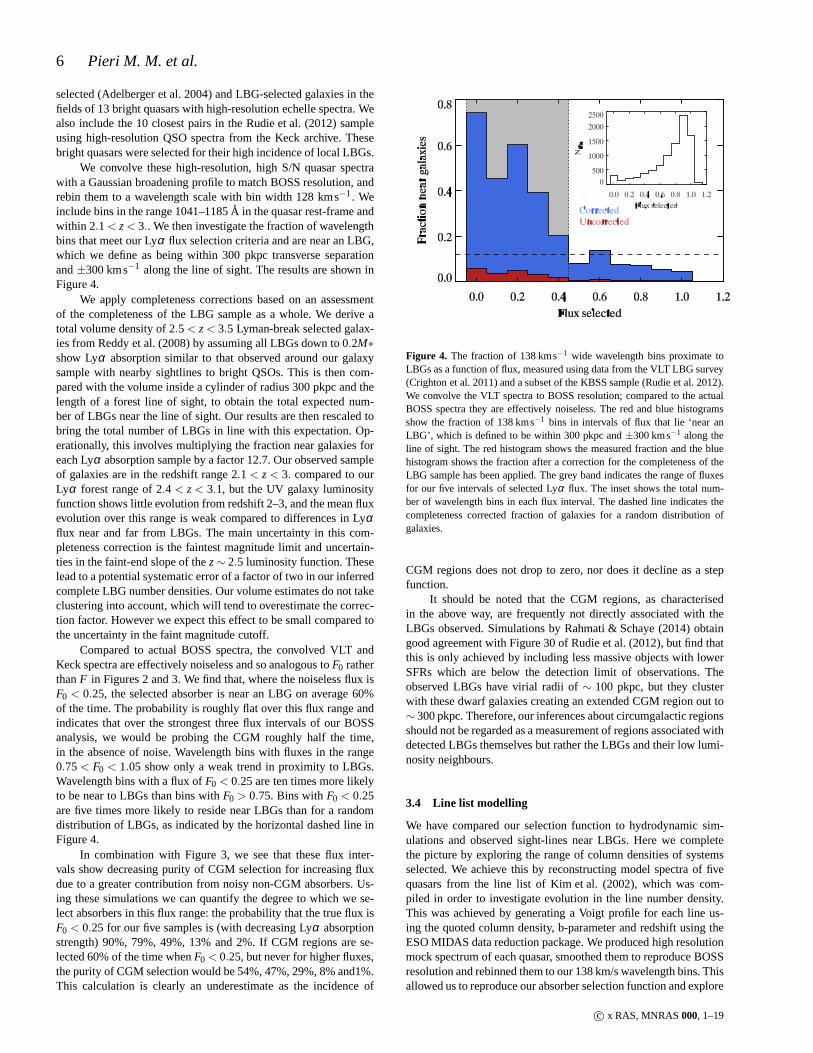
We convolve these high-resolution, high S/N quasar spectrawith a Gaussian broadening profile to match BOSS resolution,andrebin them to a wavelength scale with bin width 128 kms−1. Weinclude bins in the range 1041–1185A in the quasar rest-frame andwithin 2.1< z< 3.. We then investigate the fraction of wavelengthbins that meet our Lyα flux selection criteria and are near an LBG,which we define as being within 300 pkpc transverse separationand±300 kms−1 along the line of sight. The results are shown inFigure 4.
We apply completeness corrections based on an assessmentof the completeness of the LBG sample as a whole. We derive atotal volume density of 2.5< z< 3.5 Lyman-break selected galax-ies from Reddy et al. (2008) by assuming all LBGs down to 0.2M∗show Lyα absorption similar to that observed around our galaxysample with nearby sightlines to bright QSOs. This is then com-pared with the volume inside a cylinder of radius 300 pkpc andthelength of a forest line of sight, to obtain the total expectednum-ber of LBGs near the line of sight. Our results are then rescaled tobring the total number of LBGs in line with this expectation.Op-erationally, this involves multiplying the fraction near galaxies foreach Lyα absorption sample by a factor 12.7. Our observed sampleof galaxies are in the redshift range 2.1< z< 3. compared to ourLyα forest range of 2.4 < z< 3.1, but the UV galaxy luminosityfunction shows little evolution from redshift 2–3, and the mean fluxevolution over this range is weak compared to differences inLyαflux near and far from LBGs. The main uncertainty in this com-pleteness correction is the faintest magnitude limit and uncertain-ties in the faint-end slope of thez∼ 2.5 luminosity function. Theselead to a potential systematic error of a factor of two in our inferredcomplete LBG number densities. Our volume estimates do not takeclustering into account, which will tend to overestimate the correc-tion factor. However we expect this effect to be small compared tothe uncertainty in the faint magnitude cutoff.
Compared to actual BOSS spectra, the convolved VLT andKeck spectra are effectively noiseless and so analogous toF0 ratherthanF in Figures 2 and 3. We find that, where the noiseless flux isF0 < 0.25, the selected absorber is near an LBG on average 60%of the time. The probability is roughly flat over this flux range andindicates that over the strongest three flux intervals of ourBOSSanalysis, we would be probing the CGM roughly half the time,in the absence of noise. Wavelength bins with fluxes in the range0.75< F0 < 1.05 show only a weak trend in proximity to LBGs.Wavelength bins with a flux ofF0 < 0.25 are ten times more likelyto be near to LBGs than bins withF0 > 0.75. Bins withF0 < 0.25are five times more likely to reside near LBGs than for a randomdistribution of LBGs, as indicated by the horizontal dashedline inFigure 4.
In combination with Figure 3, we see that these flux inter-vals show decreasing purity of CGM selection for increasingfluxdue to a greater contribution from noisy non-CGM absorbers.Us-ing these simulations we can quantify the degree to which we se-lect absorbers in this flux range: the probability that the true flux isF0 < 0.25 for our five samples is (with decreasing Lyα absorptionstrength) 90%, 79%, 49%, 13% and 2%. If CGM regions are se-lected 60% of the time whenF0 < 0.25, but never for higher fluxes,the purity of CGM selection would be 54%, 47%, 29%, 8% and1%.This calculation is clearly an underestimate as the incidence of
Figure 4. The fraction of 138 kms−1 wide wavelength bins proximate toLBGs as a function of flux, measured using data from the VLT LBGsurvey(Crighton et al. 2011) and a subset of the KBSS sample (Rudie et al. 2012).We convolve the VLT spectra to BOSS resolution; compared to the actualBOSS spectra they are effectively noiseless. The red and blue histogramsshow the fraction of 138 kms−1 bins in intervals of flux that lie ‘near anLBG’, which is defined to be within 300 pkpc and±300 kms−1 along theline of sight. The red histogram shows the measured fractionand the bluehistogram shows the fraction after a correction for the completeness of theLBG sample has been applied. The grey band indicates the range of fluxesfor our five intervals of selected Lyα flux. The inset shows the total num-ber of wavelength bins in each flux interval. The dashed line indicates thecompleteness corrected fraction of galaxies for a random distribution ofgalaxies.
CGM regions does not drop to zero, nor does it decline as a stepfunction.
It should be noted that the CGM regions, as characterisedin the above way, are frequently not directly associated with theLBGs observed. Simulations by Rahmati & Schaye (2014) obtaingood agreement with Figure 30 of Rudie et al. (2012), but find thatthis is only achieved by including less massive objects withlowerSFRs which are below the detection limit of observations. Theobserved LBGs have virial radii of∼ 100 pkpc, but they clusterwith these dwarf galaxies creating an extended CGM region out to∼ 300 pkpc. Therefore, our inferences about circumgalactic regionsshould not be regarded as a measurement of regions associated withdetected LBGs themselves but rather the LBGs and their low lumi-nosity neighbours.
3.4 Line list modelling
We have compared our selection function to hydrodynamic sim-ulations and observed sight-lines near LBGs. Here we completethe picture by exploring the range of column densities of systemsselected. We achieve this by reconstructing model spectra of fivequasars from the line list of Kim et al. (2002), which was com-piled in order to investigate evolution in the line number density.This was achieved by generating a Voigt profile for each line us-ing the quoted column density, b-parameter and redshift using theESO MIDAS data reduction package. We produced high resolutionmock spectrum of each quasar, smoothed them to reproduce BOSSresolution and rebinned them to our 138 km/s wavelength bins. Thisallowed us to reproduce our absorber selection function andexplore
c© x RAS, MNRAS000, 1–19
Probing the Circumgalactic Medium at High-Redshift7
the HI column densities of lines that contributed to these absorbers,again in essentially noiseless spectra.
We argued in the previous two sections that our strongest threeabsorption samples are characterised as circumgalactic byvirtueof their selection of noiselessF0 < 0.25 wavelength bins on 138kms−1 scales, and they do so with varying degrees of efficiencydue to BOSS noise. We identified 78 of these wavelength bins overa redshift path of∆z= 2.39 and found that this sample typicallyconsists of blends of three lines which are distinct in high resolutionspectra. The highest column density line of the blend was in therange 1014cm−2 <NHI < 1016cm−2 in 94% of cases. This indicatesthat our sample is dominated by blends of strong forest lines.
The number of wavelength bins withF < 0.25 over our to-tal redshift path∆z= 3409 is 82412 (for our three strongest Lyαabsorption samples plus those bins withF < −0.05). This corre-sponds to an incidence rate ofl(z) = 24.2 with SDSS noise, com-pared tol(z) = 31.3 of effectively noise free data from our linelist model spectra. The difference can be accounted for by a 77%completeness ofF < 0.25 systems in our sample - a value which isconsistent with the signal-to-noise of our sample.
Kim et al. (2002) state that they are not able to confirm thepresence ofNHI > 1017cm−2 lines. They reconstruct the full Lyαforest, but in these cases they will underestimate the column. If weconservatively assume that all systems withNHI > 1017cm−2 aresufficiently blended with lower column lines such that they are allselected, we can assess their maximal potential impact. We alsoassume that they are selected independently and are not blendedwith each other. Fumagalli et al. (2013) find that the incidence perunit redshift of lines with a Lyman limit opacity aboveτLL = 2 (i.e.NHI > 1017.5cm−2) is l(z) = 1.21. This would mean that there are2.9 systems in our line list model spectra i.e. 3.7% of the sample.Note that this analysis includes the contribution of super Lymanlimit systems (or sub-DLAs) and DLAs. Since we have excludedthe Noterdaeme et al. (2012) DLA sample (withNHI > 1020.3cm−2)from our analysis, the above constitutes a 10% over-estimate of theincidence rate of high Lyman limit opacity systems in our sample(taking the relative incidence rate of O’Meara et al. 2013).
We may also consider the contribution of partial Lymanlimit systems withτLL > 0.5 (i.e. N > 1016.9cm−2) using theO’Meara et al. (2013) incidence rate of such systems;l(z) = 2.0in this more inclusive range. Again, we can conservatively assume100% selection in our line list model blended only with non-LLsystems. This would provide 4.8 systems and so 6.1% of the sam-ple.
It is clear even in a conservative assessment, that systems withsignificant Lyman limit opacity (τLL > 0.5 ) are a small minority ofsystems selected. However, we recognise that a small minority ofsystems with strong metal signal could have a significant impact onmeasurements of metal lines in our composite spectra. We discussthe the impact of this effect in Section 6.1.
4 STACKING PROCEDURE
We follow the procedure described in P10 to stack absorbers in theLyα forest that are selected as described in the previous section. Allabsorbers are assumed to arise due to the Lyman-α transition1, andso are assigned a suitable redshift,zabs, and shifted to the absorberrest-frame. In the process the whole quasar absorption spectrum is
1 See Section 5.2 for a discussion of where this assumption breaks down.
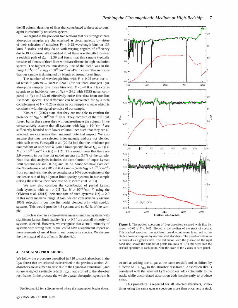
Figure 5. The stacked spectrum of Lyα absorbers selected with flux be-tween−0.05 6 F < 0.05. Plotted is the median of the stack of spectra.This stacked spectrum has not been pseudo-continuum fitted and so in-cludes broad absorption by uncorrelated absorbers. The pseudo-continuumis overlaid as a green curve. The red curve, with the y-scale on the righthand side, shows the number of pixels (in units of 103) that went into thestacked spectrum at each point. Note the scale of the y-axes in each panel.
treated as arising due to gas at the same redshift and so shifted bya factor of 1+ zabs to the absorber rest-frame. Absorption that iscorrelated with the selected Lyα absorbers adds coherently to thestack, while uncorrelated absorption adds incoherently toproducenoise.
This procedure is repeated for all selected absorbers, some-times using the same quasar spectrum more than once, and a stack
c© x RAS, MNRAS000, 1–19
8 Pieri M. M. et al.
of spectra is obtained. This wavelength grid of the stacked spectrumis set by the standard SDSS wavelength solution,
10−4 = log10λi+1− log10λi (2)
whereλ is the wavelength inA. If we select an absorber atλ1 andassume it is a Lyα forest absorber, we have a redshiftz1 given by
λ1 = λα (z1+1). (3)
Assuming that the adjacent pixel in the composite at wavelengthλ ′ > λα also measures the properties of the same gas (and so is atthe same redshift) then
λ2 = λ ′(z1+1). (4)
Substituting these into equation (2),
10−4 = log10[λ′(z1+1)]− log10[λα(z1+1)] (5)
= log10λ ′− log10λα (6)
Hence the pixel-spacing of the wavelength solution in the stackedspectrum is identical to the data where the data has a uniform∆ logλ solution. The wavelength solution of the stacked spectrumis fully described by this pixel-spacing and the rest-framewave-length of the system stacked (Lyα in this paper). Consequently theoperation of stacking is a simple process of shifting by the numberof pixels separating the marker location in the quasar spectrum andLyα in the rest-frame in the stack, with no interpolation. We rebinour spectra for Lyα selection by a factor of 2 to reduce noise. How-ever, we do not rebin the spectra before stacking. As a consequence,1215.67A in the wavelength solution for the composite spectrumis centred between two pixels. In the results that follow, the fullprofiles of lines in the composite spectra are measured without re-binning, and the central fluxes of lines are measured by averagingthe two nearest pixels in the composite (see Section 5.1).
The next step is to characterise this stack of spectra with a cho-sen statistic. We use two statistics: the median and the 3% clippedarithmetic mean (i.e. discarding the highest 3% and the lowest 3%fluxes). In both cases we determine the error estimate in a pixel bybootstrapping the stack of spectra.
Redward of 1215.67A in the composite spectrum, the stackof the spectra transitions from entirely within the forest to entirelyoutside the forest. Noise due to uncorrelated contaminating absorp-tion is the same order of magnitude as the corrected pipelineerrorestimate in the forest-contaminated portion of the stack ofspec-tra and is subdominant outside of the forest. There is significantpixel-to-pixel covariance in composite spectra due to thiscontami-nating absorption, since contaminating lines extend over resolutionelement scales. This transition region is dictated by the redshift ofthe selected Lyα absorbers with respect to the emission redshiftof the quasars in whose spectra they reside. We may choose to re-quire that only forest-free regions contribute to some portion ofthis transition region by eliminating the contribution of some ab-sorbers from that portion of the stack. We do so where the reduc-tion of noise from eliminating contaminating absorption exceedsthe increase of noise from having fewer spectra. In practicethisbalance occurs at wavelengths> 1293A. In effect, for portions ofthe composite spectrum with wavelengthλcomp> 1293A, we re-quire that(1+zabs) > (1+zq)λα/λcomp. Figure 5 presents the re-sultant stacked spectrum, and a discontinuity due to this conditionis clearly visible.
The red line in Figure 5 shows the number of spectra that con-tribute to the stacked spectrum at each point. The decline incountsat the red and blue ends are a consequence of limited spectralcov-erage in individual spectra. The lowest redshift absorbersstacked
do not have coverage at the blue end and the highest redshift ab-sorbers do not have coverage in the red end. As a consequence themean redshift is higher by∆z= 0.2 at the blue end of the stackedspectrum compared to the red end in our results.
These raw stacked spectra show smooth flux trends related tothe mean flux decrement of largely uncorrelated absorbers; theseare clearly undesirable features when producing compositespec-tra of selected absorbers. There are also smooth trends where thestacked spectrum exceeds unity by around 1%. These deviations inour stacked spectra as shown in Figure 5 (and not our compositespectra of forest absorbers such as that shown in Figure 6) are aconsequence of smooth systematic errors in spline fitting ofindi-vidual spectra.
In producing our final composite spectra, we correct boththese effects by fitting this ‘pseudo-continuum’ and removing itin keeping with the manner in which these uncorrelated absorberscontaminate the desired signal. In P10, we argued that contaminat-ing absorption typically occurs within the same resolutionelement,but would not overlap with the measured transition if fully resolved.Hence, their effect is more accurately described as additive in fluxdecrement rather than additive in optical depth. As a resultwe in-crease the flux globally by the flux decrement of these regionsinan additive manner, i.e. the desired composite spectrum is
F = Fs+(1−Fc), (7)
where Fs is the raw stacked spectrum andFc is the pseudo-continuum. We fit this pseudo-continuum by manually selectingnodes and taking a spline of these nodes. An example pseudo-continuum is shown as a green line in Figure 5. We mask knownabsorption lines from this process to prevent misleading the eye.This pseudo-continuum fitting procedure introduces errorsof orderthe size of the error estimate in the composite spectrum. In order totake this effect into account, we sum these two sources of error inquadrature in the error estimate carried forward for the compositespectra, increasing the noise-per-pixel by
√2.
Broad absorption features produced by clustering are diffi-cult to disentangle from the pseudo-continuum. In particular, theLyα feature in the strongest composite spectra shows signal outto ∼ 3000 kms−1 (in agreement with McDonald et al. 2006 andPalanque-Delabrouille et al. 2013). We fit through these large-scalefeatures in producing the pseudo-continuum, but this is a some-what subjective exercise. This effect leads to an uncertainty in themeasurement of the strongest Lyα features in our analysis, but wedemonstrate in the following section that our inference of HI col-umn is not sensitive to the measurement of Lyα or Lyβ in compos-ite spectra.
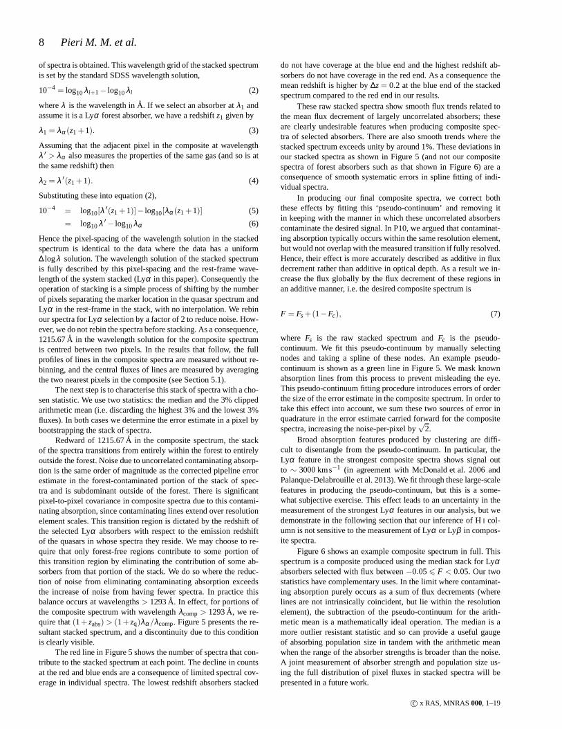
Figure 6 shows an example composite spectrum in full. Thisspectrum is a composite produced using the median stack for Lyαabsorbers selected with flux between−0.056 F < 0.05. Our twostatistics have complementary uses. In the limit where contaminat-ing absorption purely occurs as a sum of flux decrements (wherelines are not intrinsically coincident, but lie within the resolutionelement), the subtraction of the pseudo-continuum for the arith-metic mean is a mathematically ideal operation. The median is amore outlier resistant statistic and so can provide a usefulgaugeof absorbing population size in tandem with the arithmetic meanwhen the range of the absorber strengths is broader than the noise.A joint measurement of absorber strength and population size us-ing the full distribution of pixel fluxes in stacked spectra will bepresented in a future work.
c© x RAS, MNRAS000, 1–19
Probing the Circumgalactic Medium at High-Redshift9
Figure 6. Composite spectrum of Lyα absorbers selected with flux between−0.056 F < 0.05 produced using the median statistic. Error bars are showninblue. Vertical dashed lines indicate metal lines identifiedand dotted vertical lines denote the locations of the Lyman series. All lines measured for all Lyαsamples are presented in Figures A1 and A2. Note the scale of the y-axis in each panel: this is our lowest S/N composite spectrum and yet we measureabsorption features with depth as small as 0.0005.
5 RESULTS
The BOSS resolution element is broader than the width of observedLyα forest and metal lines in high-resolution spectra, so even in asingle pixel of the stacked spectrum the absorption arises from gasthat is clustered. Furthermore, the absorption features inour com-posite spectra are substantially broader than the width dictated bythe resolution element in all cases. All Lyman series features have aFWHM > 300 kms−1, in cases where it can be reliably measured,and all our metal lines show a contribution from clustering at leastas large as BOSS instrumental broadening across the full profiles(see Tables A2 and A1).
As a consequence we may integrate over the full line profilesand so include all measured clustering, or limit our integration tothe minimum degree of clustering set by the 138 kms−1 scale ofour Lyα selection bin (which is approximately the FWHM of theresolution element). We adopt the full line profile approachas ourfiducial method, denoted by subscriptf , and also consider mea-surements of the central wavelength bin of our features and denotethem with subscriptc.
5.1 H I Absorption
We characterise the HI absorption by measuring Lyman series linespresent in the stacked spectra and complement this with a measure-ment of the Lyman limit opacity provided by a modified stackingapproach.
5.1.1 Lyman series lines
We measure the absorber rest equivalent width (W) as shown inFigure 7. This measurement is normalised by the oscillator strength( f ) and the wavelength (λ ) in order to produce a quantity thatasymptotes to a constant value when the lines in the series becomeunsaturated. This quantity is measured for each of seven Lymanseries lines for both composite spectra produced using the medianand the arithmetic mean statistic. Precision measurementsof theequivalent width are challenging for the Lyα line (and Lyβ lineto a lesser degree) due to systematic errors in distinguishing thepseudo-continuum from these broad features produced by cluster-ing as discussed in the previous section.
We produce model line profiles using the analysis package
c© x RAS, MNRAS000, 1–19
10 Pieri M. M. et al.
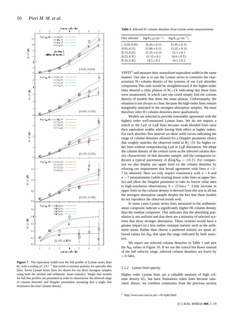
Figure 7. The equivalent width over the full profile of Lyman series linesWf with a scaling of( f λ)−1 that yields a constant quantity for optically thinlines. Seven Lyman series lines are shown for our three strongest samplesusing both the median and arithmetic mean statistics. Single line modelsfor full line profiles are presented in order to characterisethe allowed rangeof column densities and Doppler parameters assuming that a single linedominates the total column density.
Table 1. Inferred HI column densities from Lyman series measurements.
Flux selected logNf ,HI(cm−2) logNc,HI(cm−2)
[−0.05,0.05) 16.45±0.15 15.95±0.15[0.05,0.15) 15.80±0.15 15.55±0.15[0.15,0.25) 15.55±0.15 15.1±0.1[0.25,0.35) 15.15±0.1 14.6±0.15[0.35,0.45) 14.5±0.2 14.1±0.2
VPFIT2 and measure their normalised equivalent width in the samemanner. Our aim is to use the Lyman series to constrain the char-acteristic HI column density of the systems of our Lyα absorbercomposites.This task would be straightforward if the higher-orderlines showed a clear plateau inWf / f λ indicating that these lineswere unsaturated, in which case one could simply find the columndensity of models that show the same plateau. Unfortunately, thesituation is not always so clear, because the high-order lines remainmarginally saturated in the strongest absorption samples.We musttherefore infer HI column densities more qualitatively.
Models are selected to provide reasonable agreement with thehighest order well-measured Lyman lines. We do not require amatch to the Lyα or Lyβ lines because weak blended lines raisetheir equivalent widths while having little effect at higher orders.For each absorber flux interval we show solid curves indicating therange of column densities allowed for a Doppler parameter choicethat roughly matches the observed trend inWf / f λ for higher or-der lines without overproducing Lyα or Lyβ absorption. We adoptthe column density of the central curve as the inferred column den-sity characteristic of that absorber sample, and the comparison in-dicates a typical uncertainty of∆ logNHI = ±0.15. For compari-son we also display our upper limit on the column densities byrelaxing our requirement that broad agreement with linesn =3–7 be obtained. Here we only require consistency withn = 6 andn= 7 measurements (while treating lower order lines as upper lim-its) and allow the Doppler parameter to take its lowest valueseenin high-resolution observations,b = 15 kms−1. Little increase inupper limit on the column density is derived from this test inall butthe strongest absorption sample despite the fact that thesemodelsdo not reproduce the observed trends well.
In some cases Lyman series lines measured in the arithmeticmean composite indicate a significantly higher HI column densitythan the median composite. This indicates that the absorbing pop-ulation is not uniform and that there are a minority of selected sys-tems that show stronger absorption. These systems would have agreater impact on a less outlier resistant statistic such asthe arith-metic mean. Rather than choose a preferred statistic we quote al-lowed values forNHI that span the range indicated by both statis-tics.
We report our inferred column densities in Table 1 and plottheNHI values in Figure 10. If we use the central bin fluxes insteadof the full velocity range, inferred column densities are lower by∼ 0.5dex.
5.1.2 Lyman limit opacity
Higher order Lyman lines are a valuable measure of high col-umn density HI, but have limitations when lines become satu-rated. Hence, we combine constraints from the previous section
2 http://www.ast.cam.ac.uk/∼rfc/vpfit.html
c© x RAS, MNRAS000, 1–19
Probing the Circumgalactic Medium at High-Redshift11
h
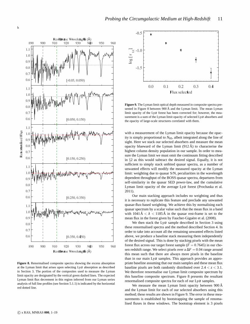
Figure 8. Renormalised composite spectra showing the excess absorptionat the Lyman limit that arises upon selecting Lyα absorption as describedin Section 3. The portion of the composites used to measure the Lymanlimit opacity are designated by the vertical green dashed lines. The expectedLyman limit flux decrement in this region inferred from our Lyman seriesanalysis of full line profiles (see Section 5.1.1) is indicated by the horizontalred dotted line.
Figure 9.The Lyman limit optical depth measured in composite spectrapre-sented in Figure 8 between 900A and the Lyman limit. The mean Lymanlimit opacity of the Lyα forest has been corrected for; however, the mea-surement is a sum of the Lyman limit opacity of selected Lyα absorbers andthe opacity of large-scale structures correlated with them.
with a measurement of the Lyman limit opacity because the opac-ity is simply proportional toNHI , albeit integrated along the line ofsight. Here we stack our selected absorbers and measure the meanopacity blueward of the Lyman limit (912A) to characterise thehighest column density population in our sample. In order tomea-sure the Lyman limit we must omit the continuum fitting describedin §2 as this would subtract the desired signal. Equally, it is notsufficient to simply stack unfitted quasar spectra, as a number ofunwanted effects will modify the measured opacity at the Lymanlimit: weighting due to quasar S/N, peculiarities in the wavelengthdependent throughput of the BOSS quasar spectra, departures fromself-similarity in the quasar SED power-law, and the cumulativeLyman limit opacity of the average Lyα forest (Prochaska et al.2011).
Our main stacking approach includes no weighting and thusit is necessary to replicate this feature and preclude any unwantedquasar-flux-based weighting. We achieve this by normalising eachquasar spectrum by a scalar value such that the mean flux in a bandwith 1041A < λ < 1185A in the quasar rest-frame is set to themean flux in the forest given by Faucher-Giguere et al. (2008).
We then stack the Lyα sample described in Section 3 usingthese renormalised spectra and the method described Section 4. Inorder to take into account all the remaining unwanted effects listedabove, we produce a baseline stack measuring them independentlyof the desired signal. This is done by stacking pixels with the meanforest flux across our target forest sample (F = 0.7645) in our cho-sen redshift range. We select pixels over a∆F = 0.04 range aroundthis mean such that there are always more pixels in the baselinethan in our main Lyα samples. This approach provides an appro-priate baseline assuming that our main samples and these mean fluxbaseline pixels are both randomly distributed over 2.4 < z< 3.1.We therefore renormalise our Lyman limit composite spectrum bythis baseline composite spectrum. Figure 8 presents the resultantrenormalised composite spectra for each of our Lyα samples.
We measure the mean Lyman limit opacity between 900Aand the Lyman limit for each of our selected absorbers using thismethod; these results are shown in Figure 9. The error in these mea-surements is established by bootstrapping the sample of renoma-lised fluxes in these windows. The bootstrap element is 3 pixels
c© x RAS, MNRAS000, 1–19
12 Pieri M. M. et al.
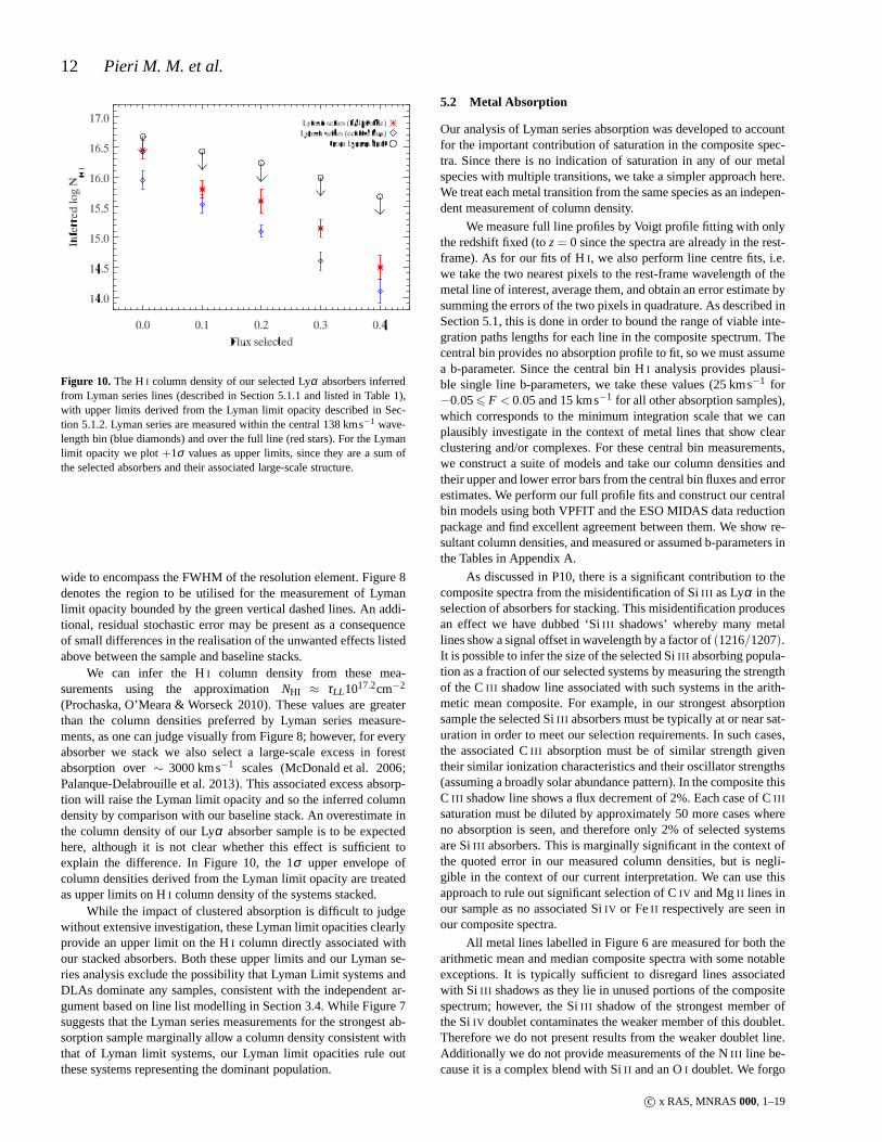
Figure 10. The HI column density of our selected Lyα absorbers inferredfrom Lyman series lines (described in Section 5.1.1 and listed in Table 1),with upper limits derived from the Lyman limit opacity described in Sec-tion 5.1.2. Lyman series are measured within the central 138kms−1 wave-length bin (blue diamonds) and over the full line (red stars). For the Lymanlimit opacity we plot+1σ values as upper limits, since they are a sum ofthe selected absorbers and their associated large-scale structure.
wide to encompass the FWHM of the resolution element. Figure8denotes the region to be utilised for the measurement of Lymanlimit opacity bounded by the green vertical dashed lines. Anaddi-tional, residual stochastic error may be present as a consequenceof small differences in the realisation of the unwanted effects listedabove between the sample and baseline stacks.
We can infer the HI column density from these mea-surements using the approximationNHI ≈ τLL1017.2cm−2
(Prochaska, O’Meara & Worseck 2010). These values are greaterthan the column densities preferred by Lyman series measure-ments, as one can judge visually from Figure 8; however, for everyabsorber we stack we also select a large-scale excess in forestabsorption over∼ 3000 kms−1 scales (McDonald et al. 2006;Palanque-Delabrouille et al. 2013). This associated excess absorp-tion will raise the Lyman limit opacity and so the inferred columndensity by comparison with our baseline stack. An overestimate inthe column density of our Lyα absorber sample is to be expectedhere, although it is not clear whether this effect is sufficient toexplain the difference. In Figure 10, the 1σ upper envelope ofcolumn densities derived from the Lyman limit opacity are treatedas upper limits on HI column density of the systems stacked.
While the impact of clustered absorption is difficult to judgewithout extensive investigation, these Lyman limit opacities clearlyprovide an upper limit on the HI column directly associated withour stacked absorbers. Both these upper limits and our Lymanse-ries analysis exclude the possibility that Lyman Limit systems andDLAs dominate any samples, consistent with the independentar-gument based on line list modelling in Section 3.4. While Figure 7suggests that the Lyman series measurements for the strongest ab-sorption sample marginally allow a column density consistent withthat of Lyman limit systems, our Lyman limit opacities rule outthese systems representing the dominant population.
5.2 Metal Absorption
Our analysis of Lyman series absorption was developed to accountfor the important contribution of saturation in the composite spec-tra. Since there is no indication of saturation in any of our metalspecies with multiple transitions, we take a simpler approach here.We treat each metal transition from the same species as an indepen-dent measurement of column density.
We measure full line profiles by Voigt profile fitting with onlythe redshift fixed (toz= 0 since the spectra are already in the rest-frame). As for our fits of HI, we also perform line centre fits, i.e.we take the two nearest pixels to the rest-frame wavelength of themetal line of interest, average them, and obtain an error estimate bysumming the errors of the two pixels in quadrature. As described inSection 5.1, this is done in order to bound the range of viableinte-gration paths lengths for each line in the composite spectrum. Thecentral bin provides no absorption profile to fit, so we must assumea b-parameter. Since the central bin HI analysis provides plausi-ble single line b-parameters, we take these values (25 kms−1 for−0.056 F < 0.05 and 15 kms−1 for all other absorption samples),which corresponds to the minimum integration scale that we canplausibly investigate in the context of metal lines that show clearclustering and/or complexes. For these central bin measurements,we construct a suite of models and take our column densities andtheir upper and lower error bars from the central bin fluxes and errorestimates. We perform our full profile fits and construct our centralbin models using both VPFIT and the ESO MIDAS data reductionpackage and find excellent agreement between them. We show re-sultant column densities, and measured or assumed b-parameters inthe Tables in Appendix A.
As discussed in P10, there is a significant contribution to thecomposite spectra from the misidentification of SiIII as Lyα in theselection of absorbers for stacking. This misidentification producesan effect we have dubbed ‘SiIII shadows’ whereby many metallines show a signal offset in wavelength by a factor of(1216/1207).It is possible to infer the size of the selected SiIII absorbing popula-tion as a fraction of our selected systems by measuring the strengthof the CIII shadow line associated with such systems in the arith-metic mean composite. For example, in our strongest absorptionsample the selected SiIII absorbers must be typically at or near sat-uration in order to meet our selection requirements. In suchcases,the associated CIII absorption must be of similar strength giventheir similar ionization characteristics and their oscillator strengths(assuming a broadly solar abundance pattern). In the composite thisC III shadow line shows a flux decrement of 2%. Each case of CIII
saturation must be diluted by approximately 50 more cases whereno absorption is seen, and therefore only 2% of selected systemsare SiIII absorbers. This is marginally significant in the context ofthe quoted error in our measured column densities, but is negli-gible in the context of our current interpretation. We can use thisapproach to rule out significant selection of CIV and MgII lines inour sample as no associated SiIV or FeII respectively are seen inour composite spectra.
All metal lines labelled in Figure 6 are measured for both thearithmetic mean and median composite spectra with some notableexceptions. It is typically sufficient to disregard lines associatedwith Si III shadows as they lie in unused portions of the compositespectrum; however, the SiIII shadow of the strongest member ofthe SiIV doublet contaminates the weaker member of this doublet.Therefore we do not present results from the weaker doublet line.Additionally we do not provide measurements of the NIII line be-cause it is a complex blend with SiII and an OI doublet. We forgo
c© x RAS, MNRAS000, 1–19
Probing the Circumgalactic Medium at High-Redshift13
presenting any potentially misleading results as these challengingmeasurements are the only available transition of NIII . The SiIIand OI transitions associated with this blend are also excluded inour analysis.
Each line is measured independently in order to make con-sistency checks possible for both full line and centre fits. However,we must modify our approach in cases of line blends. Our approachfor full line fits is illustrated in Figures A1 and A2, where the redcurve shows the fit region. For the blending of the CIV doublet wefit each line separately and omit the central overlap region.Wheretwo lines are blended such that it is not possible to measure themindependently we perform a joint fit. We make this modification forthe blend of CII and OVI at≈ 1037A and the blend of OI and SiIIat≈ 1303A.
We make no special arrangements for measuring the centralflux when lines are blended. We do, however, require that the adja-cent line has a negligible contribution to the flux in the central bin.This situation is true in all cases but one: we discard the measure-ment of the central wavelength bin for CII due to its blend withO VI .
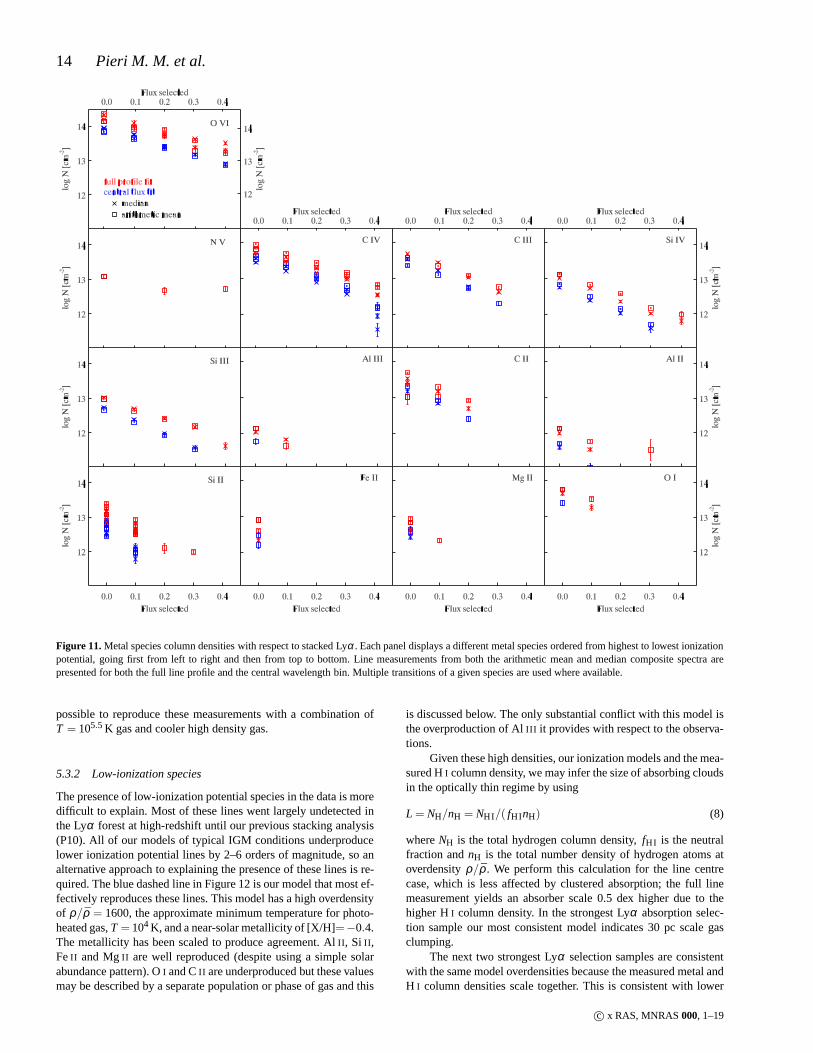
We present our metal line measurements in Figure 11 and theTables in Appendix A, conservatively excluding all measurementswith less than 5σ significance. The central flux approach showsfewer measurements as a consequence of this restriction andthefact that this approach discards some signal. Overall the narrow ve-locity range integration of the central bin approach provides resultsroughly 0.5 dex lower than the full profile measurements. SeeSec-tion 6 for a discussion of the significance of this difference.
Where multiple transitions of the same species are availablethey provide a useful alternative indication of the error inmeasur-ing lines. Their broadly good agreement indicates that we are notobserving saturated metal absorbers that are diluted by noisy selec-tion. Even a small population of very strong (F . 0.5) but not fullysaturated metal lines is ruled out. For example, the ratio ofdou-blet line strengths of 2:1 in lithium-like ions (e.g. OVI ) is a ratio inopacities and not flux; hence a very strong doublet that is diluted bynon-detections to appear as a weak doublet in the composite spec-trum would have a measurably different doublet ratio from that ofa ubiquitous, weak doublet.
We treat measurements of the arithmetic mean and the me-dian as two measurements of the same systems. The comparisonbetween these two statistics is, to a limited extent, an indicationof population size amongst the stack, particularly outsideof theLyα forest where the distribution of contaminating absorptionismuch larger than the stack. The question of absorber populationsizes (i.e. what fraction of the selected Lyα systems are contribut-ing to a given metal line) will be addressed in a future publication.
5.3 Comparison to simple models
The column densities of metal species in the intergalactic and cir-cumgalactic media depend upon metallicity, abundance patternsand ionization. Changes in metallicity of the observed gas will scaleall our measured columns globally, while changes in abundancepattern will scale our measurements element-by-element. Changesin ionization will modify metal line column densities in a set ofbroad, but constrained, ways, and it is upon ionization thatwe fo-cus here. We treat metallicity as a free parameter and assumesolarabundance patterns in this publication.
The ionization of all these elements is dictated by gas density,temperature, ionising radiation, and geometry. Geometry is onlyof significance when gas is self-shielded. We neglect this effect
since, as we demonstrated in Section 5.1, all our samples aredom-inated by gas with an insufficient HI column to be self-shielding.Even our most conservative estimates of the potential impact of asubsample of self-shielded systems show them to be sub-dominant(Section 6.1).
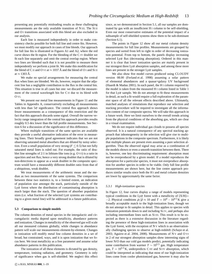
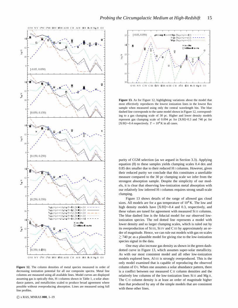
The points in Figure 12 show all our metal column densitymeasurements for full line profiles. Measurements are grouped byspecies and sorted from left to right in order of decreasing ioniza-tion potential. From top to bottom, the panels display increasingselected Lyα flux (decreasing absorption). Ordered in this man-ner it is clear that lower ionization species are mainly present inour strongest three Lyα absorption samples, and among these morelines are present in the stronger Lyα samples.
We also show five model curves produced using CLOUDYversion 08.00 (Ferland et al. 1998) assuming a solar patternof elemental abundances and a quasar+galaxy UV background(Haardt & Madau 2001). In each panel, the HI column required bythe model is taken from the measured HI column listed in Table 1for that Lyα sample. We do not attempt to fit these measurementsin detail, as such a fit would require a full exploration of theparam-eter space of all the relevant effects described above. Ultimately,matched analyses of simulations that reproduce our selection andstacking procedure will be required to investigate all the informa-tion content of our composite spectra. We will take this approach ina future work. Here we limit ourselves to the overall trends arisingfrom the physical conditions of the absorbing gas, which areclearin a visual examination.
We do not require individual gas clouds to possess all speciesobserved. It is a natural consequence of any spectral stacking ap-proach that inhomogeneity in the selection will give rise tomulti-ple populations in the composite spectrum. Furthermore, itis likelythat multiple phases are present even assuming a pure selection al-gorithm. Thus the observed signal may arise as a combinationofthe models shown or even a smooth transition between them. Thereis, however, one key discriminating requirement: absorption mustnot be overproduced by a given model. If a model reproduces theabsorption for a particular species, it must not overproduce absorp-tion for another species in order to be viable. Only full lineprofilemeasurements are shown here, but the line centre approach pro-duces similar results since both the HI and metal column densitiesare lower by approximately the same factor.
5.3.1 High-ionization species
In Figure 12, four curves display a range of models representingtypical conditions in the Lyα forest with a metallicity of [X/H]=−2. Physical conditionsρ/ρ ≈ 10 andT = 104 − 104.5 K give abroadly acceptable match to the high-ionization lines, though wedo not attempt to fit samples in detail. This applies to species withionization potentials down to and including SiIV , and perhaps alsoincluding intermediate lines such as SiIII . This result is to be ex-pected as there is a extensive discussion in the literature regard-ing the presence of these high-ionization lines in association withthe Lyα forest, with the exception of NV which is an observation-ally challenging species to observe at high-redshift (Schaye et al.2003; Aguirre et al. 2004, 2008). Measurements of NV and OVI
in 2 of our strongest absorption samples show interesting signs oflower N/O than our cold gas models predict, potentially indicatingsome contribution from warmerT ∼ 105.5 gas. High temperaturegas,T = 105.5 K, underpredicts CIII and SiIV absorption, whichcould be interpreted as indicating that most of our high-ionizationlines come from cooler photoionized gas, however it may alsobe
c© x RAS, MNRAS000, 1–19
14 Pieri M. M. et al.
Figure 11.Metal species column densities with respect to stacked Lyα . Each panel displays a different metal species ordered fromhighest to lowest ionizationpotential, going first from left to right and then from top to bottom. Line measurements from both the arithmetic mean and median composite spectra arepresented for both the full line profile and the central wavelength bin. Multiple transitions of a given species are used where available.
possible to reproduce these measurements with a combination ofT = 105.5 K gas and cooler high density gas.
5.3.2 Low-ionization species
The presence of low-ionization potential species in the data is moredifficult to explain. Most of these lines went largely undetected inthe Lyα forest at high-redshift until our previous stacking analysis(P10). All of our models of typical IGM conditions underproducelower ionization potential lines by 2–6 orders of magnitude, so analternative approach to explaining the presence of these lines is re-quired. The blue dashed line in Figure 12 is our model that most ef-fectively reproduces these lines. This model has a high overdensityof ρ/ρ = 1600, the approximate minimum temperature for photo-heated gas,T = 104 K, and a near-solar metallicity of [X/H]=−0.4.The metallicity has been scaled to produce agreement. AlII , Si II ,FeII and MgII are well reproduced (despite using a simple solarabundance pattern). OI and CII are underproduced but these valuesmay be described by a separate population or phase of gas and this
is discussed below. The only substantial conflict with this model isthe overproduction of AlIII it provides with respect to the observa-tions.
Given these high densities, our ionization models and the mea-sured HI column density, we may infer the size of absorbing cloudsin the optically thin regime by using
L = NH/nH = NHI/( fHInH) (8)
whereNH is the total hydrogen column density,fHI is the neutralfraction andnH is the total number density of hydrogen atoms atoverdensityρ/ρ . We perform this calculation for the line centrecase, which is less affected by clustered absorption; the full linemeasurement yields an absorber scale 0.5 dex higher due to thehigher HI column density. In the strongest Lyα absorption selec-tion sample our most consistent model indicates 30 pc scale gasclumping.
The next two strongest Lyα selection samples are consistentwith the same model overdensities because the measured metal andH I column densities scale together. This is consistent with lower
c© x RAS, MNRAS000, 1–19
Probing the Circumgalactic Medium at High-Redshift15
Figure 12. The column densities of metal species measured in order ofdecreasing ionization potential for all our composite spectra. Metal linecolumns are measured using all available lines. Model curves are displayedassuming gas is optically thin, HI columns shown in Table 1, a solar abun-dance pattern, and metallicities scaled to produce broad agreement wherepossible without overproducing absorption. Lines are measured using fullline profiles.
Figure 13. As for Figure 12, highlighting variations about the model thatmost effectively reproduces the lowest ionization lines inthe lowest fluxsample when measured using only the central wavelength bin.The bluedashed line corresponds to the same model shown in Figure 12,correspond-ing to a gas clumping scale of 30 pc. Higher and lower density modelsrepresent gas clumping scale of 0.094 pc for [X/H]=0.3 and 740 pc for[X/H]=-0.4 respectively.T = 104 K in all cases.
purity of CGM selection (as we argued in Section 3.3). Applyingequation (8) to these samples yields clumping scales 0.4 dexand0.85 dex smaller due to their reduced HI columns. However, giventheir reduced purity we conclude that this constitutes a unreliablemeasure compared to the 30 pc clumping scale we infer from thestrongest absorption sample. Despite the simplicity of ourmod-els, it is clear that observing low-ionization metal absorption withour relatively low inferred HI columns requires strong small-scaleclumping.
Figure 13 shows details of the range of allowed gas cloudsizes. All models are for a gas temperature of 104 K. The low andhigh density models have [X/H]=-0.4 and 0.3, respectively,andthese values are tuned for agreement with measured SiII columns.The blue dashed line is the fiducial model for our observed low-ionization species. The red dotted line represents a model withlower density and so larger clumping scales, which is ruled out byits overproduction of SiIII , Si IV and CIII by approximately an or-der of magnitude. Hence, we can rule out models with gas on scales& 740 pc as a plausible model for giving rise to the low-ionizationspecies signal in the data.
One may also increase gas density as shown in the green dash-dotted curve in Figure 13, which assumes super-solar metallicity.As with our most consistent model and all other low-ionizationmodels explored here, AlIII is strongly overproduced. This is theonly model examined that is capable of reproducing the observedcolumn of OI. When one assumes a solar abundance pattern, thereis a conflict between our measured CII column densities and therelatively low columns of the low-ionization lines SiII and MgII .The CII column density is at least an order of magnitude higherthan that produced by any of the simple models that are consistentwith these other lines.
c© x RAS, MNRAS000, 1–19
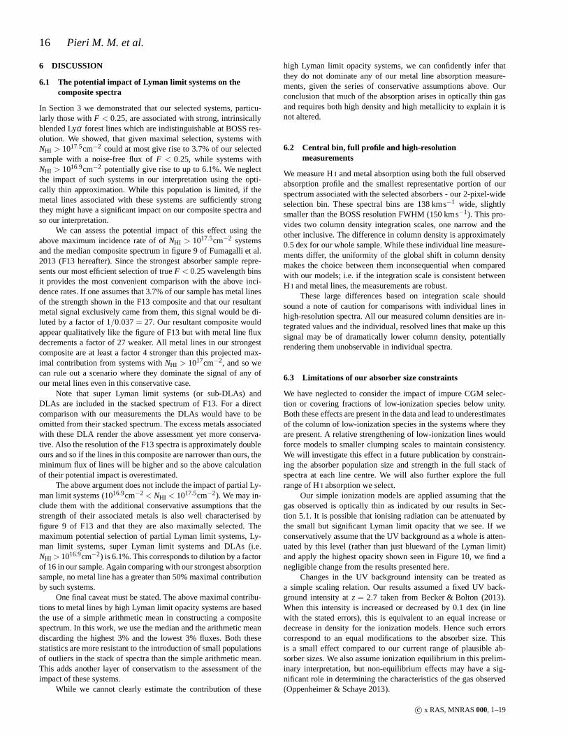
16 Pieri M. M. et al.
6 DISCUSSION
6.1 The potential impact of Lyman limit systems on thecomposite spectra
In Section 3 we demonstrated that our selected systems, particu-larly those withF < 0.25, are associated with strong, intrinsicallyblended Lyα forest lines which are indistinguishable at BOSS res-olution. We showed, that given maximal selection, systems withNHI > 1017.5cm−2 could at most give rise to 3.7% of our selectedsample with a noise-free flux ofF < 0.25, while systems withNHI > 1016.9cm−2 potentially give rise to up to 6.1%. We neglectthe impact of such systems in our interpretation using the opti-cally thin approximation. While this population is limited, if themetal lines associated with these systems are sufficiently strongthey might have a significant impact on our composite spectraandso our interpretation.
We can assess the potential impact of this effect using theabove maximum incidence rate of ofNHI > 1017.5cm−2 systemsand the median composite spectrum in figure 9 of Fumagalli et al.2013 (F13 hereafter). Since the strongest absorber sample repre-sents our most efficient selection of trueF < 0.25 wavelength binsit provides the most convenient comparison with the above inci-dence rates. If one assumes that 3.7% of our sample has metal linesof the strength shown in the F13 composite and that our resultantmetal signal exclusively came from them, this signal would be di-luted by a factor of 1/0.037= 27. Our resultant composite wouldappear qualitatively like the figure of F13 but with metal line fluxdecrements a factor of 27 weaker. All metal lines in our strongestcomposite are at least a factor 4 stronger than this projected max-imal contribution from systems withNHI > 1017cm−2, and so wecan rule out a scenario where they dominate the signal of any ofour metal lines even in this conservative case.
Note that super Lyman limit systems (or sub-DLAs) andDLAs are included in the stacked spectrum of F13. For a directcomparison with our measurements the DLAs would have to beomitted from their stacked spectrum. The excess metals associatedwith these DLA render the above assessment yet more conserva-tive. Also the resolution of the F13 spectra is approximately doubleours and so if the lines in this composite are narrower than ours, theminimum flux of lines will be higher and so the above calculationof their potential impact is overestimated.
The above argument does not include the impact of partial Ly-man limit systems (1016.9cm−2 < NHI < 1017.5cm−2). We may in-clude them with the additional conservative assumptions that thestrength of their associated metals is also well characterised byfigure 9 of F13 and that they are also maximally selected. Themaximum potential selection of partial Lyman limit systems, Ly-man limit systems, super Lyman limit systems and DLAs (i.e.NHI > 1016.9cm−2) is 6.1%. This corresponds to dilution by a factorof 16 in our sample. Again comparing with our strongest absorptionsample, no metal line has a greater than 50% maximal contributionby such systems.
One final caveat must be stated. The above maximal contribu-tions to metal lines by high Lyman limit opacity systems are basedthe use of a simple arithmetic mean in constructing a compositespectrum. In this work, we use the median and the arithmetic meandiscarding the highest 3% and the lowest 3% fluxes. Both thesestatistics are more resistant to the introduction of small populationsof outliers in the stack of spectra than the simple arithmetic mean.This adds another layer of conservatism to the assessment oftheimpact of these systems.
While we cannot clearly estimate the contribution of these
high Lyman limit opacity systems, we can confidently infer thatthey do not dominate any of our metal line absorption measure-ments, given the series of conservative assumptions above.Ourconclusion that much of the absorption arises in optically thin gasand requires both high density and high metallicity to explain it isnot altered.
6.2 Central bin, full profile and high-resolutionmeasurements
We measure HI and metal absorption using both the full observedabsorption profile and the smallest representative portionof ourspectrum associated with the selected absorbers - our 2-pixel-wideselection bin. These spectral bins are 138 kms−1 wide, slightlysmaller than the BOSS resolution FWHM (150 kms−1). This pro-vides two column density integration scales, one narrow andtheother inclusive. The difference in column density is approximately0.5 dex for our whole sample. While these individual line measure-ments differ, the uniformity of the global shift in column densitymakes the choice between them inconsequential when comparedwith our models; i.e. if the integration scale is consistentbetweenH I and metal lines, the measurements are robust.
These large differences based on integration scale shouldsound a note of caution for comparisons with individual lines inhigh-resolution spectra. All our measured column densities are in-tegrated values and the individual, resolved lines that make up thissignal may be of dramatically lower column density, potentiallyrendering them unobservable in individual spectra.
6.3 Limitations of our absorber size constraints
We have neglected to consider the impact of impure CGM selec-tion or covering fractions of low-ionization species belowunity.Both these effects are present in the data and lead to underestimatesof the column of low-ionization species in the systems wheretheyare present. A relative strengthening of low-ionization lines wouldforce models to smaller clumping scales to maintain consistency.We will investigate this effect in a future publication by constrain-ing the absorber population size and strength in the full stack ofspectra at each line centre. We will also further explore thefullrange of HI absorption we select.
Our simple ionization models are applied assuming that thegas observed is optically thin as indicated by our results inSec-tion 5.1. It is possible that ionising radiation can be attenuated bythe small but significant Lyman limit opacity that we see. If weconservatively assume that the UV background as a whole is atten-uated by this level (rather than just blueward of the Lyman limit)and apply the highest opacity shown seen in Figure 10, we find anegligible change from the results presented here.
Changes in the UV background intensity can be treated asa simple scaling relation. Our results assumed a fixed UV back-ground intensity atz= 2.7 taken from Becker & Bolton (2013).When this intensity is increased or decreased by 0.1 dex (in linewith the stated errors), this is equivalent to an equal increase ordecrease in density for the ionization models. Hence such errorscorrespond to an equal modifications to the absorber size. Thisis a small effect compared to our current range of plausible ab-sorber sizes. We also assume ionization equilibrium in thisprelim-inary interpretation, but non-equilibrium effects may have a sig-nificant role in determining the characteristics of the gas observed(Oppenheimer & Schaye 2013).
c© x RAS, MNRAS000, 1–19
Probing the Circumgalactic Medium at High-Redshift17
We provide only a preliminary exploration of strong effectsseen in our composite spectra by comparison with a limited set ofmodels. We do not consider modifications to the abundance profileof elements measured, but measurements from multiple species ofthe same element allow us to limit the importance of this effect. Inparticular, observations of only SiII , Si III and SiIV are sufficientto support the constraints on absorber sizes in the CGM, since re-producing SiII columns without overproducing our SiIII and SiIVcolumns forces models to small absorber sizes.
Our models assume a quasar+galaxy UV background model,however, much of our results arise as a consequence of probingcircumgalactic regions. Therefore, a potential source of systematicerror may arise where galaxies generate a local excess in thegalaxycomponent of this radiation field. In general, a higher amplituderadiation field would require higher gas density to compensate.
6.4 Potential for further IGM/CGM constraints
We detect signs of [C/α] > 1, and this is not the first time thatsuper solar C/α has been observed at high-redshift. Pettini et al.(2008), Penprase et al. (2010) and Cooke et al. (2011) find evi-dence of [C/α] as high as 0.5 dex above solar in metal poorDLAs. Our results show a discrepancy 0.5 dex higher still thanthese DLA observations and for much higher metallicities. Apotential explanation for these observations of high [C/α] inDLAs is a significant contribution by explosions of Pop III starsKobayashi, Tominaga & Nomoto (2011).
In addition, our observations of FeII may allow explorationof deviations from solarα/Fe. We see no significant deviationsthat are distinct from the allowed range of gas physical conditionsthus far; however, a full species-by-species exploration of param-eter space with modifications to the UV background, abundancepatterns and physical conditions would place valuable constraintson the abundance pattern of gas in the CGM at high-redshift.
The ultimate goal of these measurements is improving our un-derstanding of galaxy formation and evolution. The most effectiveway of achieving this is by direct comparison with hydrodynamicsimulations. The column densities for HI and several metal linesare broadly in line with those predicted for CGM regions by re-cent hydrodynamic simulations (Hummels et al. 2013; Shen etal.2013), but a detailed comparison is necessary for the subsetof sightlines through simulated CGM regions that meet our Lyα selectionfunctions and total HI columns. Our measurements allow a directcomparison to simulations, but they all do so with some simplifi-cations. The optimal way to explore this problem without loss ofinformation content is to compare the composite spectra with com-posites produced from simulations and we will conduct this anal-ysis in a future work (M. Mortonson et al. in prep). We enable thesimulation community to utilise these measurements in their en-tirety by providing our composite spectra online3.
6.5 Comparison with other observations
In the above analysis we have assumed that high-ionization linesarise in gas with typical IGM physical conditions rather than a cir-cumgalactic origin, even for systems which we infer arise inCGMregions (Section 3.3). We assume that we do select CGM regionsin a minority of cases or that there is a nearby excess in IGM struc-ture that we fail to resolve. However, recent results by Tripp et al.
3 http://icg.port.ac.uk/stable/pierim/compositelyabossdr9.html
(2011) and Meiring et al. (2013) show low, high and intermediateionization potential species are observed to be kinematically simi-lar despite certainly probing different phases. Although they are atlow-redshift, these results are consistent with our observations andare suggestive of poor mixing of hot and cold, metal rich and metalpoor, dense and rare gas as part of a bulk flow.
Simcoe et al. (2006) inferred near-solar metallicities andhigh-densities consistent with our results from three high-redshiftgalaxies with a line of sight in their circumgalactic regions.Schaye, Carswell & Kim (2007) explored the properties of severalstrong CIV lines and performed ionization calculations using upperlimits on column densities of various other species. The physicalconditions derived indicated clumping scales of∼ 100 pc, solar orhigher metallicities and densities of aroundnH ∼ 10−3.5cm−3 (orρ/ρ ∼ 50). The low HI columns probed (. 1014cm−2) and mod-erate densities indicate that these systems are likely intergalactic inorigin and not verifiably proximate to galaxies. The resultsare pri-marily a measurement of mixing of metals on large scales. Morerecently P10 found evidence of 10 pc clumping from compositespectra of Lyα absorbers using SDSS-II spectra. These results sug-gested near solar metallicities, high densities and low-ionizationspecies making them broadly indicative of circumgalactic regions;an inference that we verify here.
Steidel et al. (2010) detected sub-kpc clumping based on ob-servations of LBGs as background light sources near LBGs. Theyalso argue for an increase in absorber sizes with increasinggalacticimpact parameter.
Observations of MgII absorbers have shown signs of clump-ing scales∼ 10−2pc by comparison of incidence rates and beamsizes along the line of sight to gamma-ray bursts and quasars(Frank et al. 2007; Hao et al. 2007). There remains, however,con-siderable uncertainty, particularly with respect to quasar beamsizes. Indications of sub-parsec structure in MgII absorbers havebeen further reinforced by the results of Hacker et al. (2013) basedon time-variability of absorbers in SDSS quasar spectra.
At low-redshift a variety of measurements have been per-formed. Tripp et al. (2002) studied a system in the Virgo clus-ter showing substantial low-ionization lines (but a lack ofhigh-ionization lines) and concluded a sub-kpc thickness of the gas thatgave rise to them. Aracil et al. (2006) explored absorbers along theline of sight to az= 0.37 quasar and found metallicities 0.5dexbelow solar and absorber size of a few kpc. A study of NeVIII andO VI toward az= 1.0 quasar (Meiring et al. 2013) found systemswith metallicities ofZ > 0.3Z⊙ and sizes∼ 1kpc. Supersolar neonabsorption has also been seen around our galaxy (Nicastro etal.2002).
Rigby, Charlton & Churchill (2002) found indications ofclumping on ∼ 10pc scales in a sub-set of their weak MgII
absorbers that are relatively iron rich atz ∼ 1; however,Lynch & Charlton (2007) found that the incidence of such weakMg II systems is much reduced at redshifts as high asz= 2.4, thelower redshift limit of our study.
There are striking similarities between our strongest Lyα ab-sorption sample and the lowest HI column densities of Lehner et al.(2013) investigated atz. 1. These HI columns are slightly higherthan ours (& 1016.2cm−2 for their strongest component). They des-ignate such systems Lyman limit systems, while formally theyare only marginally partial Lyman limit systems. They report thatthese partial Lyman limit systems are circumgalactic in origin, andin this sample they find a bimodality in metallicity with peaksat [X/H] ≃ −1.6 and -0.3. They interpret these results as evi-dence of both clumpy metal rich outflows and cold metal poor ac-
c© x RAS, MNRAS000, 1–19
18 Pieri M. M. et al.
cretion streams. Recent metallicity measurements of componentsof the sub-damped system atz = 2.4 nearby a Lyman break-selected galaxy (Crighton, Hennawi & Prochaska 2013) show sim-ilarly high and low metallicities, which suggests that thisbimodal-ity may also be present at higher redshifts. While we cannot detectthis bimodality in our composite spectra, we are broadly consistentwith both these phases and indeed do not require additional phasesthan these two broadly defined categories.
7 SUMMARY
We present composite spectra of Lyα forest absorbers selected byflux in 138 kms−1 wide bins in the BOSS DR9 sample of quasarspectra. This binning scale represents two pixels of the SDSS wave-length solution and a little under the typical resolution ofthe BOSSspectrograph (150 kms−1). We limit ourselves to intervening ab-sorbers (selected within 1041–1185A in the quasar rest-frame) atredshifts 2.4< z< 3.1. We examine five samples with increasingflux centred atF = 0.0, 0.1, 0.2, 0.3 and 0.4.
Tests on high-resolution spectra show that our three strongestabsorbers samples would, in the absence of noise, probe CGM re-gions (300 pkpc transverse,±300 kms−1 line of sight)≈ 60% ofthe time (Figure 4). In the presence of noise, we get steadilyde-creasing purity of CGM selection with increasing flux (Figure 3).
We characterise the inferred HI column density contributionto this selection by measuring Lyman series lines and comparingthem with a variety of single line models. We complement thiswitha new modified approach to stacking directed at measuring theLy-man limit opacity resulting from our selected absorbers andany as-sociated excess Lyα absorption. We present measurements of thecolumn density of 26 metal lines from 7 elements and 13 ioniza-tion species, over the full line profiles (which includes allclusteredabsorption both from complexes and large scale structure) and forthe wavelength bin selected i.e. 138 kms−1 scales (which corre-sponds to our most exclusive measure with respect to clustering).These measurements constitute upper and lower limits on ourcol-umn density integration scale; however, both sets include clusteringmaking them difficult to compare with observations of individuallines of sight.
We compare our measurements to simple ionization modelsassuming a quasar and galaxy UV background model and a solarpattern of elemental abundances. We find that the potential contri-bution of Lyman limit systems to our metal line measurementsissufficiently weak to allow the use of the optically thin approxima-tion in our ionization corrections without modifying our interpreta-tion. All our samples show clear measurements of high-ionizationparameter lines broadly in line with physical conditions associatedwith the IGM and a metallicity of approximately [X/H]=−2. Ourcomposite spectra corresponding to CGM regions show a numberof additional lines. These are mostly low-ionization linesand weare able to reproduce them in our models only with much higherdensities and metallicities. The combination of density and columndensity implies a characteristic length scale of these low-ionizationabsorbers, and we find greatest consistency with absorbers typically30 pc in size with a near-solar metallicity of [X/H]=−0.4 . Thereare indications that measurements of OI require yet smaller scalegas clumping. We also detect tentative signs of a strongly elevatedC/α compared to solar, and note the potential to measure bothα/Feand the shape of the UV background as part of a full search of pa-rameter space.
We make available all our composite spectra available to al-
low a direct comparison between simulations and our absorptionprofiles.
ACKNOWLEDGMENTS
We would like to offer special thanks to the anonymous referee,whose constructive criticism led to significant improvement of thismanuscript. We also thank Romeel Dave, Neal Katz, BenjaminOp-penheimer and Mark Fardal for the use of their SPH simulationsand Benjamin Oppenheimer for the use of his CLOUDY look uptables. Also we thank Todd Tripp and Joop Schaye for their in-sightful comments on this work.
The research leading to these results has received fund-ing from the European Union Seventh Framework Programme(FP7/2007-2013) under grant agreement n [PIIF-GA-2011-301665]. MM was partially supported by NASA grantNNX12AG71G and CCAPP at Ohio State. DW acknowl-edges support of NSF Grant AST-1009505 and NASA ATP grantNNX10AJ95G
Funding for SDSS-III has been provided by the Alfred P.Sloan Foundation, the Participating Institutions, the National Sci-ence Foundation, and the U.S. Department of Energy Office of Sci-ence. The SDSS-III web site is http://www.sdss3.org/. SDSS-III ismanaged by the Astrophysical Research Consortium for the Partici-pating Institutions of the SDSS-III Collaboration including the Uni-versity of Arizona, the Brazilian Participation Group, BrookhavenNational Laboratory, University of Cambridge, Carnegie MellonUniversity, University of Florida, the French Participation Group,the German Participation Group, Harvard University, the Institutode Astrofisica de Canarias, the Michigan State/Notre Dame/JINAParticipation Group, Johns Hopkins University, Lawrence BerkeleyNational Laboratory, Max Planck Institute for Astrophysics, MaxPlanck Institute for Extraterrestrial Physics, New MexicoStateUniversity, New York University, Ohio State University, Pennsyl-vania State University, University of Portsmouth, Princeton Uni-versity, the Spanish Participation Group, University of Tokyo, Uni-versity of Utah, Vanderbilt University, University of Virginia Uni-versity of Washington, and Yale University.
REFERENCES
Adelberger K. L., Steidel C. C., Shapley A. E., Hunt M. P., ErbD. K., Reddy N. A., Pettini M., 2004, ApJ, 607, 226
Adelberger K. L., Steidel C. C., Shapley A. E., Pettini M., 2003,ApJ, 584, 45
Adelman-McCarthy J. K. et al., 2007, ApJS, 172, 634Aguirre A., Dow-Hygelund C., Schaye J., Theuns T., 2008, ApJ,689, 851
Aguirre A., Hernquist L., Schaye J., Weinberg D. H., Katz N.,Gardner J., 2001, ApJ, 560, 599
Aguirre A., Schaye J., Kim T.-S., Theuns T., Rauch M., SargentW. L. W., 2004, ApJ, 602, 38
Ahn C. P. et al., 2012, ApJS, 203, 21Anders E., Grevesse N., 1989, Geochim. Cosmochim. Acta, 53,197
Aracil B., Tripp T. M., Bowen D. V., Prochaska J. X., Chen H.-W.,Frye B. L., 2006, MNRAS, 367, 139
Barai P. et al., 2013, MNRAS, 430, 3213Becker G. D., Bolton J. S., 2013, ArXiv e-printsBielby R. et al., 2013, MNRAS, 430, 425
c© x RAS, MNRAS000, 1–19
Probing the Circumgalactic Medium at High-Redshift19
Bielby R. M. et al., 2011, MNRAS, 414, 2Bolton A. S. et al., 2012, AJ, 144, 144Bovy J. et al., 2011, ApJ, 729, 141Cooke R., Pettini M., Steidel C. C., Rudie G. C., Nissen P. E.,2011, MNRAS, 417, 1534
Cowie L. L., Songaila A., Kim T.-S., Hu E. M., 1995, AJ, 109,1522
Crighton N. H. M. et al., 2011, MNRAS, 414, 28Crighton N. H. M., Hennawi J. F., Prochaska J. X., 2013, ApJ,776, L18
Dawson K. S. et al., 2013, AJ, 145, 10Eisenstein D. J. et al., 2011, AJ, 142, 72Faucher-Giguere C.-A., Keres D., 2011, MNRAS, 412, L118Faucher-Giguere C.-A., Prochaska J. X., Lidz A., Hernquist L.,Zaldarriaga M., 2008, ApJ, 681, 831
Ferland G. J., Korista K. T., Verner D. A., Ferguson J. W., King-don J. B., Verner E. M., 1998, PASP, 110, 761
Frank S., Bentz M. C., Stanek K. Z., Mathur S., Dietrich M., Pe-terson B. M., Atlee D. W., 2007, Ap&SS, 312, 325
Fumagalli M., O’Meara J. M., Prochaska J. X., Worseck G., 2013,ApJ, 775, 78 F13
Fumagalli M., Prochaska J. X., Kasen D., Dekel A., Ceverino D.,Primack J. R., 2011, MNRAS, 418, 1796
Gunn J. E., Peterson B. A., 1965, ApJ, 142, 1633Gunn J. E. et al., 2006, AJ, 131, 2332Haardt F., Madau P., 2001, in Clusters of Galaxies and the HighRedshift Universe Observed in X-rays, Neumann D. M., TranJ. T. V., eds.
Hacker T. L., Brunner R. J., Lundgren B. F., York D. G., 2013,MNRAS, 434, 163
Hao H. et al., 2007, ApJ, 659, L99Hinshaw G. et al., 2009, ApJS, 180, 225Hu E. M., Kim T.-S., Cowie L. L., Songaila A., Rauch M., 1995,AJ, 110, 1526
Hummels C. B., Bryan G. L., Smith B. D., Turk M. J., 2013, MN-RAS, 430, 1548
Kim T.-S., Carswell R. F., Cristiani S., D’Odorico S., GiallongoE., 2002, MNRAS, 335, 555
Kobayashi C., Tominaga N., Nomoto K., 2011, ApJ, 730, L14Lee K.-G. et al., 2013, AJ, 145, 69Lee K.-G., Suzuki N., Spergel D. N., 2012, AJ, 143, 51Lehner N. et al., 2013, ApJ, 770, 138Lundgren B. F. et al., 2012, ApJ, 760, 49Lynch R. S., Charlton J. C., 2007, ApJ, 666, 64Lynds R., 1971, ApJ, 164, L73Mac Low M.-M., Ferrara A., 1999, ApJ, 513, 142Martin C. L., 2005, ApJ, 621, 227McDonald P. et al., 2006, ApJS, 163, 80Meiring J. D., Tripp T. M., Werk J. K., Howk J. C., Jenkins E. B.,Prochaska J. X., Lehner N., Sembach K. R., 2013, ApJ, 767, 49
Meyer D. M., York D. G., 1987, ApJ, 315, L5Nicastro F. et al., 2002, ApJ, 573, 157Nielsen N. M., Churchill C. W., Kacprzak G. G., Murphy M. T.,2013, ArXiv e-prints
Noterdaeme P. et al., 2012, A&A, 547, L1O’Meara J. M., Prochaska J. X., Worseck G., Chen H.-W., MadauP., 2013, ApJ, 765, 137
Oppenheimer B. D., Dave R., 2006, MNRAS, 373, 1265Oppenheimer B. D., Dave R., 2008, MNRAS, 387, 577Oppenheimer B. D., Schaye J., 2013, MNRAS, 434, 1043Palanque-Delabrouille N. et al., 2013, A&A acceptedParis I. et al., 2012, A&A, 548, A66
Penprase B. E., Prochaska J. X., Sargent W. L. W., Toro-MartinezI., Beeler D. J., 2010, ApJ, 721, 1
Pettini M., Zych B. J., Steidel C. C., Chaffee F. H., 2008, MNRAS,385, 2011
Pieri M. M., Frank S., Mathur S., Weinberg D. H., York D. G.,Oppenheimer B. D., 2010a, ApJ, 716, 1084
Pieri M. M., Frank S., Weinberg D. H., Mathur S., York D. G.,2010b, ApJ, 724, L69 P10
Pieri M. M., Haehnelt M. G., 2004, MNRAS, 347, 985Pieri M. M., Martel H., 2007, ApJ, 662, L7Pieri M. M., Martel H., Grenon C., 2007, ApJ, 658, 36Pieri M. M., Schaye J., Aguirre A., 2006, ApJ, 638, 45Pinsonneault S., Martel H., Pieri M. M., 2010, ApJ, 725, 2087Prochaska J. X., O’Meara J. M., Worseck G., 2010, ApJ, 718, 392Rahmati A., Schaye J., 2014, MNRAS, 438, 529Rakic O., Schaye J., Steidel C. C., Rudie G. C., 2012, ApJ, 751,94
Reddy N. A., Steidel C. C., Pettini M., Adelberger K. L., ShapleyA. E., Erb D. K., Dickinson M., 2008, ApJS, 175, 48
Rigby J. R., Charlton J. C., Churchill C. W., 2002, ApJ, 565, 743Ross N. P. et al., 2012, ApJS, 199, 3Rudie G. C. et al., 2012, ApJ, 750, 67Scannapieco E., Ferrara A., Madau P., 2002, ApJ, 574, 590Schaye J., Aguirre A., Kim T.-S., Theuns T., Rauch M., SargentW. L. W., 2003, ApJ, 596, 768
Schaye J., Carswell R. F., Kim T.-S., 2007, MNRAS, 379, 1169Schaye J. et al., 2010, MNRAS, 402, 1536Schaye J., Rauch M., Sargent W. L. W., Kim T.-S., 2000, ApJ,541, L1
Shen S., Madau P., Guedes J., Mayer L., Prochaska J. X., WadsleyJ., 2013, ApJ, 765, 89
Simcoe R. A., Sargent W. L. W., Rauch M., 2004, ApJ, 606, 92Simcoe R. A., Sargent W. L. W., Rauch M., Becker G., 2006, ApJ,637, 648
Smee S. A. et al., 2013, AJ, 146, 32Springel V., 2005, MNRAS, 364, 1105Steidel C. C., Erb D. K., Shapley A. E., Pettini M., Reddy N.,Bogosavljevic M., Rudie G. C., Rakic O., 2010, ApJ, 717, 289
Stocke J. T., Keeney B. A., Danforth C. W., Shull J. M., FroningC. S., Green J. C., Penton S. V., Savage B. D., 2013, ApJ, 763,148
Tripp T. M. et al., 2002, ApJ, 575, 697Tripp T. M. et al., 2011, Science, 334, 952Tumlinson J. et al., 2011, Science, 334, 948York D. G. et al., 2000, AJ, 120, 1579
APPENDIX A: METAL LINE MEASUREMENTS
c© x RAS, MNRAS000, 1–19
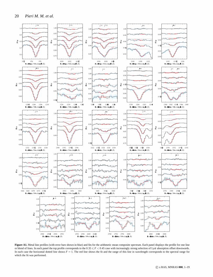
20 Pieri M. M. et al.
Figure A1. Metal line profiles (with error bars shown in blue) and fits forthe arithmetic mean composite spectrum. Each panel displays the profile for one lineor blend of lines. In each panel the top profile corresponds tothe 0.356 F < 0.45 case with increasingly strong selection of Lyα absorption offset downwards.In each case the horizontal dotted line showsF = 1. The red line shows the fit and the range of this line in wavelength corresponds to the spectral range forwhich the fit was performed.
c© x RAS, MNRAS000, 1–19
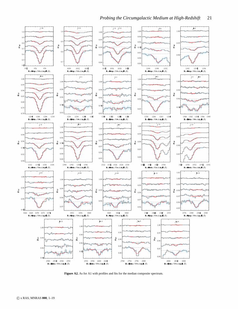
Probing the Circumgalactic Medium at High-Redshift21
Figure A2. As for A1 with profiles and fits for the median composite spectrum.
c© x RAS, MNRAS000, 1–19
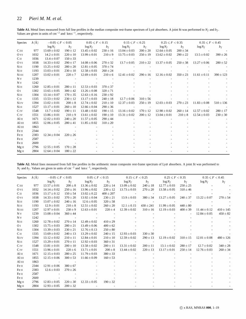
22 Pieri M. M. et al.
Table A1. Metal lines measured from full line profiles in the median composite rest-frame spectrum of Lyα absorbers. A joint fit was performed toNf andbf .Values are given in units of cm−2 and kms−1, respectively.
Species λ(A) −0.056 F < 0.05 0.056 F < 0.15 0.156 F < 0.25 0.256 F < 0.35 0.356 F < 0.45logNf bf logNf bf logNf bf logNf bf logNf bf
C III 977 13.69±0.02 190±12 13.45±0.02 230±16 13.04±0.03 200±20 12.64±0.05 200±34 - -O VI 1032 14.2±0.01 220±10 13.99±0.01 210±9 13.75±0.03 250±19 13.62±0.02 290±22 13.5±0.02 390±26C II 1036 13.4±0.07 150±33 - - - - - - - -O VI 1038 14.33±0.02 290±17 14.08±0.06 270±32 13.7±0.05 210±22 13.37±0.05 250±38 13.27±0.06 280±52Si II 1190 13.25±0.02 280±20 12.81±0.05 370±74 - - - - - -Si II 1193 13.03±0.01 230±10 12.58±0.03 260±24 - - - - - -Si III 1207 13.02±0.01 220±7 12.69±0.01 210±6 12.41±0.02 290±16 12.16±0.02 350±23 11.61±0.11 390±123N V 1239 - - - - - - - - - -N V 1242 - - - - - - - - - -Si II 1260 12.85±0.01 280±11 12.53±0.03 370±37 - - - - - -O I 1302 13.65±0.05 300±42 13.26±0.08 320±71 - - - - - -Si II 1304 13.14±0.07 170±35 12.63±0.16 230±92 - - - - - -C II 1335 13.53±0.02 230±12 13.17±0.03 240±18 12.7±0.06 310±56 - - - -Si IV 1394 13.02±0.01 200±8 12.74±0.02 210±10 12.37±0.03 250±19 12.03±0.03 270±23 11.83±0.08 510±136Si II 1527 13.17±0.01 260±10 12.66±0.04 290±36 - - - - - -C IV 1548 13.7±0.02 190±11 13.48±0.02 190±15 13.16±0.02 170±12 12.98±0.02 260±14 12.57±0.02 280±17C IV 1551 13.86±0.01 210±9 13.61±0.02 190±10 13.31±0.02 200±12 13.04±0.01 210±8 12.54±0.03 230±30Al II 1671 12.02±0.03 240±20 11.57±0.05 290±44 - - - - - -Al III 1855 12.06±0.05 280±41 11.85±0.02 310±20 - - - - - -Al III 1863 - - - - - - - - - -FeII 2344 - - - - - - - - - -FeII 2383 12.34±0.04 220±26 - - - - - - - -FeII 2587 - - - - - - - - - -FeII 2600 - - - - - - - - - -Mg II 2796 12.55±0.05 170±28 - - - - - - - -Mg II 2804 12.64±0.04 180±22 - - - - - - - -
Table A2. Metal lines measured from full line profiles in the arithmetic mean composite rest-frame spectrum of Lyα absorbers. A joint fit was performed toNf andbf . Values are given in units of cm−2 and kms−1, respectively.
Species λ(A) −0.056 F < 0.05 0.056 F < 0.15 0.156 F < 0.25 0.256 F < 0.35 0.356 F < 0.45logNf bf logNf bf logNf bf logNf bf logNf bf
C III 977 13.57±0.01 200±8 13.36±0.02 220±14 13.09±0.02 240±18 12.77±0.03 250±25 - -O VI 1032 14.14±0.02 250±16 13.96±0.02 230±12 13.73±0.03 270±20 13.58±0.05 310±46 - -C II 1036 13.17±0.12 150±54 13.02±0.22 400±207 - - - - - -O VI 1038 14.33±0.02 370±20 13.92±0.04 230±21 13.9±0.03 380±34 13.27±0.05 240±37 13.22±0.07 270±54Si II 1190 13.07±0.02 240±16 12.6±0.05 320±58 - - - - - -Si II 1193 12.9±0.01 210±8 12.51±0.02 260±20 12.1±0.15 430±241 11.99±0.05 440±80 - -Si III 1207 12.97±0.01 230±9 12.63±0.01 220±4 12.39±0.02 310±16 12.19±0.03 400±39 11.44±0.12 410±145N V 1239 13.08±0.04 360±44 - - - - - - 12.84±0.05 450±82N V 1242 - - - - - - - - - -Si II 1260 12.78±0.02 270±14 12.49±0.02 410±29 - - - - - -O I 1302 13.75±0.03 280±21 13.49±0.06 400±62 - - - - - -Si II 1304 13.39±0.03 230±21 12.76±0.13 250±80 - - - - - -C II 1335 13.69±0.02 240±13 13.29±0.02 240±15 12.93±0.03 330±30 - - - -Si IV 1394 13.12±0.02 210±11 12.84±0.01 210±10 12.59±0.02 290±13 12.19±0.02 310±15 12.01±0.08 480±126Si II 1527 13.29±0.01 270±11 12.92±0.03 360±31 - - - - - -C IV 1548 13.81±0.01 200±10 13.58±0.02 200±11 13.31±0.02 200±11 13.1±0.02 280±17 12.7±0.02 340±28C IV 1551 13.96±0.01 220±6 13.71±0.01 200±8 13.44±0.02 220±13 13.17±0.01 250±14 12.76±0.03 260±34Al II 1671 12.15±0.03 280±25 11.79±0.03 380±33 - - - - - -Al III 1855 12.15±0.06 300±53 11.66±0.09 160±53 - - - - - -Al III 1863 - - - - - - - - - -FeII 2344 12.91±0.06 380±67 - - - - - - - -FeII 2383 12.6±0.03 270±26 - - - - - - - -FeII 2587 - - - - - - - - - -FeII 2600 - - - - - - - - - -Mg II 2796 12.83±0.05 220±30 12.33±0.05 190±32 - - - - - -Mg II 2804 12.93±0.05 200±32 - - - - - - - -
c© x RAS, MNRAS000, 1–19
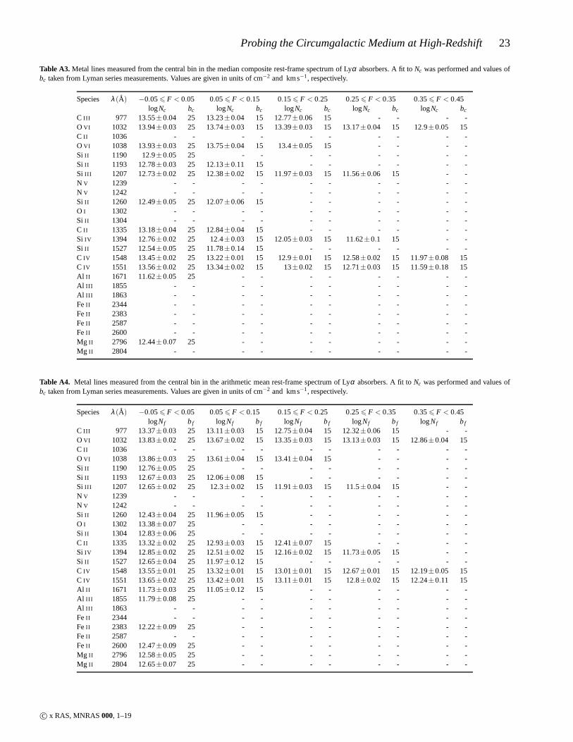
Probing the Circumgalactic Medium at High-Redshift23
Table A3. Metal lines measured from the central bin in the median composite rest-frame spectrum of Lyα absorbers. A fit toNc was performed and values ofbc taken from Lyman series measurements. Values are given in units of cm−2 and kms−1, respectively.
Species λ(A) −0.056 F < 0.05 0.056 F < 0.15 0.156 F < 0.25 0.256 F < 0.35 0.356 F < 0.45logNc bc logNc bc logNc bc logNc bc logNc bc
C III 977 13.55±0.04 25 13.23±0.04 15 12.77±0.06 15 - - - -O VI 1032 13.94±0.03 25 13.74±0.03 15 13.39±0.03 15 13.17±0.04 15 12.9±0.05 15C II 1036 - - - - - - - - - -O VI 1038 13.93±0.03 25 13.75±0.04 15 13.4±0.05 15 - - - -Si II 1190 12.9±0.05 25 - - - - - - - -Si II 1193 12.78±0.03 25 12.13±0.11 15 - - - - - -Si III 1207 12.73±0.02 25 12.38±0.02 15 11.97±0.03 15 11.56±0.06 15 - -N V 1239 - - - - - - - - - -N V 1242 - - - - - - - - - -Si II 1260 12.49±0.05 25 12.07±0.06 15 - - - - - -O I 1302 - - - - - - - - - -Si II 1304 - - - - - - - - - -C II 1335 13.18±0.04 25 12.84±0.04 15 - - - - - -Si IV 1394 12.76±0.02 25 12.4±0.03 15 12.05±0.03 15 11.62±0.1 15 - -Si II 1527 12.54±0.05 25 11.78±0.14 15 - - - - - -C IV 1548 13.45±0.02 25 13.22±0.01 15 12.9±0.01 15 12.58±0.02 15 11.97±0.08 15C IV 1551 13.56±0.02 25 13.34±0.02 15 13±0.02 15 12.71±0.03 15 11.59±0.18 15Al II 1671 11.62±0.05 25 - - - - - - - -Al III 1855 - - - - - - - - - -Al III 1863 - - - - - - - - - -FeII 2344 - - - - - - - - - -FeII 2383 - - - - - - - - - -FeII 2587 - - - - - - - - - -FeII 2600 - - - - - - - - - -Mg II 2796 12.44±0.07 25 - - - - - - - -Mg II 2804 - - - - - - - - - -
Table A4. Metal lines measured from the central bin in the arithmetic mean rest-frame spectrum of Lyα absorbers. A fit toNc was performed and values ofbc taken from Lyman series measurements. Values are given in units of cm−2 and kms−1, respectively.
Species λ(A) −0.056 F < 0.05 0.056 F < 0.15 0.156 F < 0.25 0.256 F < 0.35 0.356 F < 0.45logNf bf logNf bf logNf bf logNf bf logNf bf
C III 977 13.37±0.03 25 13.11±0.03 15 12.75±0.04 15 12.32±0.06 15 - -O VI 1032 13.83±0.02 25 13.67±0.02 15 13.35±0.03 15 13.13±0.03 15 12.86±0.04 15C II 1036 - - - - - - - - - -O VI 1038 13.86±0.03 25 13.61±0.04 15 13.41±0.04 15 - - - -Si II 1190 12.76±0.05 25 - - - - - - - -Si II 1193 12.67±0.03 25 12.06±0.08 15 - - - - - -Si III 1207 12.65±0.02 25 12.3±0.02 15 11.91±0.03 15 11.5±0.04 15 - -N V 1239 - - - - - - - - - -N V 1242 - - - - - - - - - -Si II 1260 12.43±0.04 25 11.96±0.05 15 - - - - - -O I 1302 13.38±0.07 25 - - - - - - - -Si II 1304 12.83±0.06 25 - - - - - - - -C II 1335 13.32±0.02 25 12.93±0.03 15 12.41±0.07 15 - - - -Si IV 1394 12.85±0.02 25 12.51±0.02 15 12.16±0.02 15 11.73±0.05 15 - -Si II 1527 12.65±0.04 25 11.97±0.12 15 - - - - - -C IV 1548 13.55±0.01 25 13.32±0.01 15 13.01±0.01 15 12.67±0.01 15 12.19±0.05 15C IV 1551 13.65±0.02 25 13.42±0.01 15 13.11±0.01 15 12.8±0.02 15 12.24±0.11 15Al II 1671 11.73±0.03 25 11.05±0.12 15 - - - - - -Al III 1855 11.79±0.08 25 - - - - - - - -Al III 1863 - - - - - - - - - -FeII 2344 - - - - - - - - - -FeII 2383 12.22±0.09 25 - - - - - - - -FeII 2587 - - - - - - - - - -FeII 2600 12.47±0.09 25 - - - - - - - -Mg II 2796 12.58±0.05 25 - - - - - - - -Mg II 2804 12.65±0.07 25 - - - - - - - -
c© x RAS, MNRAS000, 1–19