Lecture 25

Vibrating circular membrane (conclusion)

Some normal modes of vibration

Relevant section of text: 7.8.3 (p. 320-1)

We now examine a few normal modes of vibration of the circular drum. Recall that they are given

by

umn(r, θ, t) = fmn(r)gm(θ)hmn(t), m = 0, 1, 2, · · · , (1)

where

fmn(r) = Jm(√

λmnr),

gm(θ) = am cos mθ + bm sin mθ,

hmn(t) = cmn cos(√

λmnct) + dmn sin(√

λmnct). (2)

In order to reduce the complexity, we’ll consider a simplified form of the above solutions which does

not change the general qualitative properties of the modes of vibration. First we’ll set am = 1 and

bm = 0 – this only changes the orientation of the mode in the xy-plane. Second, we’ll set cmn = 1 and

dmn = 0. This corresponds to zero initial velocity.

Case 1: m = 0

In this case, the normal modes are given by (up to a constant)

u0,n(r, θ) = J0(√

λ0,nr) cos(√

λ0,nct), (3)

where

λ0,n =(z0,n

a

)2, n = 1, 2, · · · , (4)

where z0,n denotes the nth positive zero of J0(z). The frequencies of oscillation of these normal modes

are given by

ω0,n =√

λ0,nc =z0,n

ac. (5)

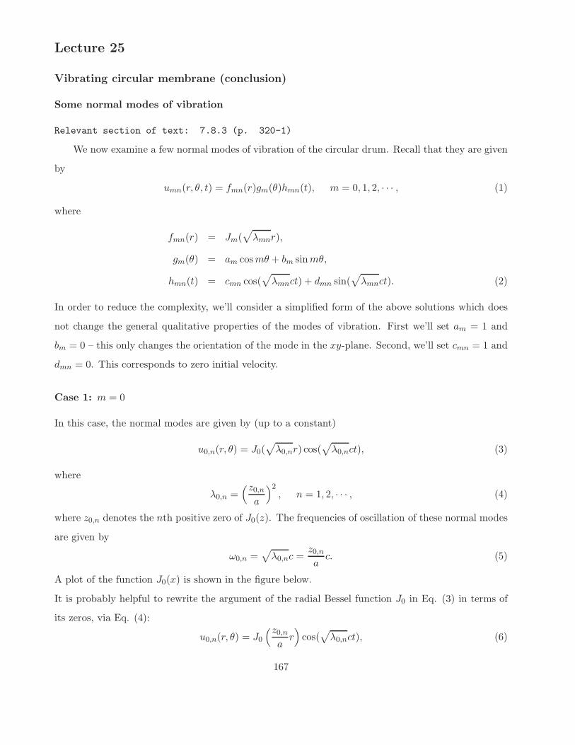
A plot of the function J0(x) is shown in the figure below.

It is probably helpful to rewrite the argument of the radial Bessel function J0 in Eq. (3) in terms of

its zeros, via Eq. (4):

u0,n(r, θ) = J0

(z0,n

ar)

cos(√

λ0,nct), (6)

167

-1

-0.75

-0.5

-0.25

0

0.25

0.5

0.75

1

0 1 2 3 4 5 6 7 8 9 10 11 12 13 14 15 16 17 18 19 20

x

Bessel function J_0(x)

In this way, we see that when r = a, the argument of J0 will be one of its zeros, thereby ensuring that

its value is zero, in accordance with the clamped boundary condition.

Case 1(a): n = 1 Here, the first zero z0,1 has been chosen. Note that J0(z) > 0 for 0 ≤ z < z0,1,

which translates to u0,1(r) > 0 for 0 ≤ r < a. Rotating the graph of J0(z) for 0 ≤ z ≤ z0,1 about

the y-axis yields a scaled picture of the drum’s membrane at maximum amplitude. Consequently, all

points on the membrane travel upward and downward in unison – a kind of two-dimensional analogue

to the lowest mode of the one-dimensional vibrating string. There are no nodes for r < a.

Case 1(b): n = 2 If we choose the second zero z0,2 of J0(z), then rotating the graph of J0(z) for

0 ≤ x ≤ z0,2 about the yaxis gives a picture of the drum membrane at the instant that points are at

their maximum distance from equilibrium. It is not too hard to show that the circle of points

r =z0,1

z0,2a ≈ 0.44a (7)

is a set of nodal points with zero amplitude. A convenient way to picture this is from the top:

+

−

Choosing higher zeros x0,k will introduce more nodal circles into the modes. Plots of the normal

modes for m = 0, n = 1, 2, 3 are shown in the textbook by Haberman, p. 321.

168

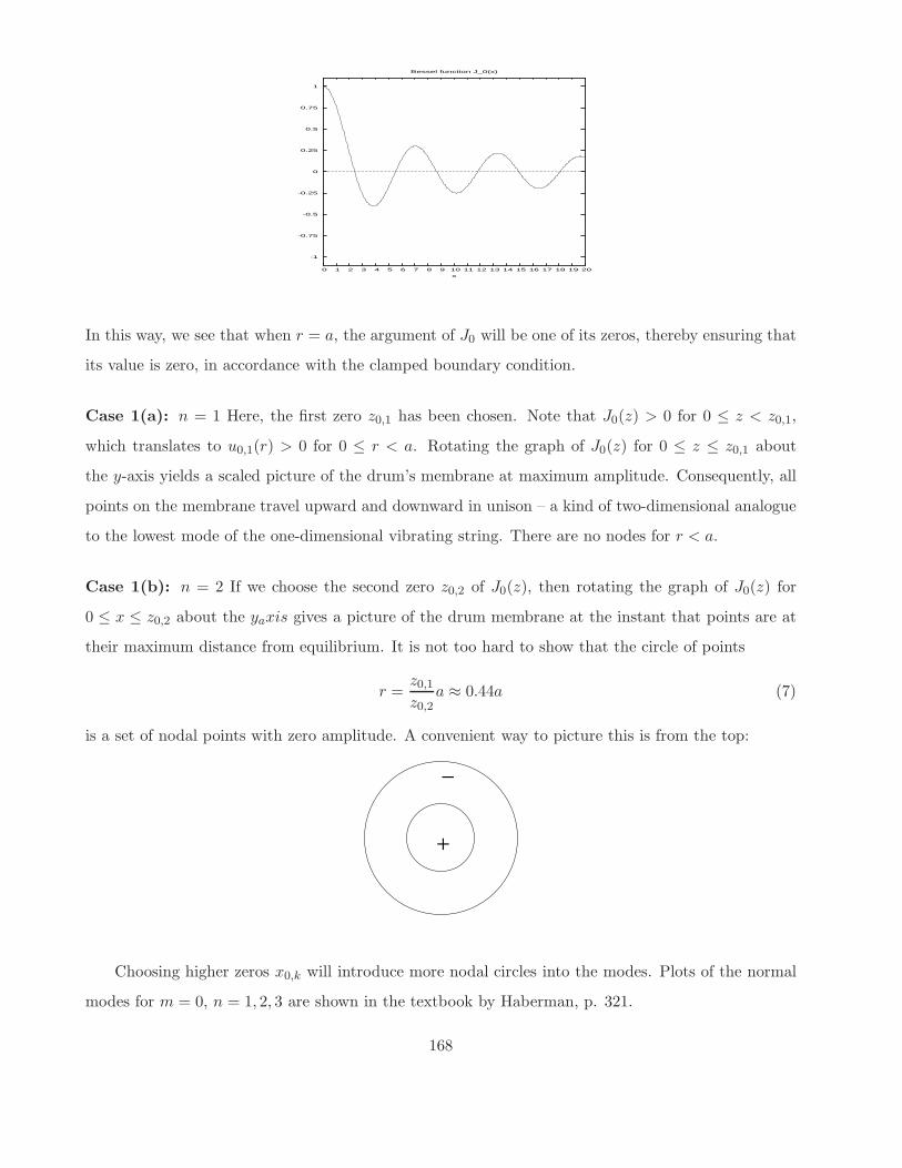
Case 2: m = 1

We must now choose the Bessel function J1(z) to form the radial part of the displacement function:

u1,n(r, θ) = J1(√

λ1,nr) cos(θ) cos(√

λ1,nct), (8)

Let us first examine the θ-dependent portion of the mode, namely, cos(θ). Note that cos(θ) > 0 for

−π/2 < θ < π/2 and S(θ) < 0 for π/2 < θ < 3π/2. As well cos(θ) = 0 for θ = π/2 and θ = 3π/2 which

correspond to a vertical nodal line. We can depict the positive and negative regions schematically as

follows:

+−

The function cos(θ) will be multiplied by the radial function J1(√

λ1,nr) to give the amplitude

function of the vibrational mode.

Case 2(a): n = 1 When we choose n = 1, the first zero of J1(z), then the radial function J1(√

λ1,1r)

is nonnegative. This means that the displacements will be positive and negative as in the above figure.

Case 2(b): n = 2 In the case n = 2, the function J1(z) produces positive and negative regions in

roughly the same way as was done for J0(z) above. J1(z) > 0 for 0 < z < z1,1 and J1(z) < 0 for

z1,1 < z < z1,2. Multiplication of these regions with the positive and negative regions associated with

S(θ) = cos θ gives the following pattern:

+ −−+

169

One can, of course, continue this procedure and use higher zeros z1,n of J1(z).

Finally, plots of the normal modes for the cases m = 3, n = 1, 2, are presented in the text by

Haberman, p. 321.

Infinite Domain Problems / Fourier Transform Solutions of PDEs

Relevant section of textbook: 10.2

We now wish to consider PDEs over infinite intervals, e.g., the entire real line (−∞,∞) or the

half-line [0,∞). One may well ask, “Why?” After all, physical problems are finite in nature. To a

good approximation, however, many problems are “infinite” as far as their consituents are concerned.

For example, to an electron situated near the center of a charged plate of dimensions, say, 1 m by 1

m, the plate is essentially infinite in size. Indeed, even if this plate were 1 mm by 1 mm, the plate

would be infinite – in other words, the effects of the boundaries would not be noticed.

The formulation of problems over infinite intervals is a way to eliminate the effects of boundaries.

In many situations, such a formulation is a good approximation.

We first consider solutions to the heat equation on the real line, i.e.,

∂u

∂t= k

∂2u

∂x2, x ∈ (−∞,∞). (9)

We’ll need a set of initial conditions, i.e.,

u(x, 0) = f(x), x ∈ (−∞,∞). (10)

As for boundary conditions, we shall assume that

u(x, t) → 0 as x → ±∞. (11)

These boundary conditions are homogeneous, which naturally leads to the question of whether the

method of separation of variables will work here. The answer is “Yes,” but with some interesting

consequences.

We begin with another look at the separation of variables method over the finite interval [0, L].

Recall that assuming a solution of the form

u(x, t) = φ(x)h(t) (12)

170

yields the ODEs

h′ + λkh = 0 (13)

and

φ′′ + λφ = 0. (14)

You’ll recall that physically useful solutions exist for λ > 0.

Instead of accomodating any definite boundary conditions at this time, we simply write the gen-

eral solutions φn(x) that correspond to the eigenvalues λn = nπ/L and which form a complete and

orthogonal set on [0, L]:

φn(x) = an cos(nπx

L

)

+ bn sin(nπx

L

)

. (15)

Associated with these functions are the time-dependent functions,

hn(t) = e−kλnt = e−k(nπ/L)2t. (16)

The normal modes produced by these solutions are

un(x, t) = φn(x)hn(t), n = 0, 1, · · · , (17)

so that the general solution of the heat equation is given by

u(x, t) =

∞∑

n=0

un(x, t), (18)

or

u(x, t) =

∞∑

n=0

[

an cos(nπx

L

)

+ bn sin(nπx

L

)]

e−k(nπ/L)2t. (19)

The expansion coefficients are given by

a0 =1

L

∫ L

0f(x) dx =

2

LA0,

an =2

L

∫ L

0f(x) cos

(nπx

L

)

dx =2

LAn,

bn =2

L

∫ L

0f(x) sin

(nπx

L

)

dx =2

LBn. (20)

In this way, the general solution may be written as

u(x, t) =

∞∑

n=0

2

L

[

An cos(nπx

L

)

+ Bn sin(nπx

L

)]

e−k(nπ/L)2t. (21)

171

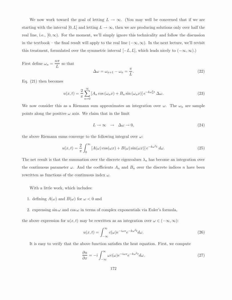
We now work toward the goal of letting L → ∞. (You may well be concerned that if we are

starting with the interval [0, L] and letting L → ∞, then we are producing solutions only over half the

real line, i.e., [0,∞). For the moment, we’ll simply ignore this technicality and follow the discussion

in the textbook – the final result will apply to the real line (−∞,∞). In the next lecture, we’ll revisit

this treatment, formulated over the symmetric interval [−L,L], which leads nicely to (−∞,∞).)

First define ωn =nπ

Lso that

∆ω = ωn+1 − ωn =π

L. (22)

Eq. (21) then becomes

u(x, t) =2

π

∞∑

n=0

[An cos (ωnx) + Bn sin (ωnx)] e−kω2nt ∆ω. (23)

We now consider this as a Riemann sum approximates an integration over ω. The ωn are sample

points along the positive ω axis. We claim that in the limit

L → ∞ → ∆ω → 0, (24)

the above Riemann sums converge to the following integral over ω:

u(x, t) =2

π

∫

∞

0[A(ω) cos(ωx) + B(ω) sin(ωx)] e−kω2t dω. (25)

The net result is that the summation over the discrete eigenvalues λn has become an integration over

the continuous parameter ω. And the coefficients An and Bn over the discrete indices n have been

rewritten as functions of the continuous index ω.

With a little work, which includes:

1. defining A(ω) and B(ω) for ω < 0 and

2. expressing sin ω and cos ω in terms of complex exponentials via Euler’s formula,

the above expression for u(x, t) may be rewritten as an integration over ω ∈ (−∞,∞):

u(x, t) =

∫

∞

−∞

c(ω)e−iωxe−kω2tdω. (26)

It is easy to verify that the above function satisfies the heat equation. First, we compute

∂u

∂x= −i

∫

∞

−∞

ωc(ω)e−iωxe−kω2tdω. (27)

172

Differentiating once again yields

∂2u

∂x2= −

∫

∞

−∞

ω2c(ω)e−iωxe−kω2tdω. (28)

Partial differentiation of u(x, t) with respect to t yields

∂u

∂t= −k

∫

∞

−∞

ω2c(ω)e−iωxe−kω2tdω

= k∂2u

∂x2. (29)

From Eq. (26), the initial condition is given by

u(x, 0) = f(x) =

∫

∞

−∞

c(ω)e−iωx dω. (30)

The above “derivations” were rather informal and certainly not rigorous. In the next lecture, we

shall provide a little more justification for the integral form of the solution u(x, t) in Eq. (26).

173

Lecture 26

Infinite Domain Problems/Fourier Transform Solutions of PDEs (cont’d)

Relevant section of textbook: 10.3

Consider the interval I = [−L,L] ⊂ R. It is a basic fact of Fourier analysis that the functions

un(x) = e−inπx/L, · · · ,−1, 0, 1, · · · , (31)

form an orthogonal set on [−L,L] under the inner product

〈u, v〉 =

∫ L

−Lu∗(x)v(x) dx, u, v : I → C, u, v ∈ L2(I). (32)

Here, u and v are complex-valued functions and u∗ denotes the complex conjugate of u. (It is

more convenient to work with the complex-valued exponentials – we don’t have to deal with sin

and cos functions separately. The above result is equivalent to the statement that the set of functions{

sinnπx

L, cos

nπx

L

}

∞

n=0forms an orthogonal set on I = [−L,L].)

Let us prove the orthogonality of the un: In the case that n 6= m,

〈un, um〉 =

∫ L

−Leinπx/Le−imπx/Ldx

=

∫ L

−Lei(n−m)πx/Ldx

=1

i(n − m)

L

π

[

ei(n−m)πx/L]L

−L

=1

i(n − m)

L

π

[

ei(n−m)π − e−i(n−m)π]

=2L

(n − m)πsin(n − m)π

= 0. (33)

In the case that n = m,

〈un, un〉 =

∫ L

−Leinπx/Le−inπx/Ldx

=

∫ L

−Ldx

= 2L. (34)

It is also a fact that the functions un(x) defined above form a complete set of functions on the

interval I = [−L,L]: We should specify that this set is complete in the space of complex-valued

functions L2(I) with inner product defined above.

174

Now let f(x) be a real-valued function defined on I. We’re assuming that f(x) is real-valued

in light of future applications – it will serve as the initial distribution of temperatures for the heat

equation. We shall also assume that f ∈ L2(I). This is not a strong assumption – in most applications,

f(x) will be either continuous or piecewise continuous on I.

The completeness of the set of functions {un}∞n=−∞implies that

f(x) =

∞∑

n=−∞

cnun =

∞∑

n=−∞

cne−inπx/L, (35)

where

cn =〈un, f〉〈un, un〉

=1

2L

∫ L

−Leinπx/Lf(x) dx. (36)

The equality in Eq. (35) is to be understood in the L2 sense – it implies that∥

∥

∥

∥

∥

f(x) −∞

∑

n=−∞

cne−inπx/L

∥

∥

∥

∥

∥

= 0. (37)

In the special case that f is continuous at x, the equality holds in the strict sense – the infinite sum

converges to the value of f at x. In the case that f is discontinuous at x, the infinite sum converges

to the average of the left and right limits of f at x. This is written in the textbook as follows,

f(x+) + f(x−)

2=

∞∑

n=−∞

cne−inπx/L. (38)

Let us now return to Eqs. (35) and (36). We substitute the latter into the former as follows:

f(x) =

∞∑

n=−∞

1

2L

[∫ L

−Lf(s)einπs/Lds

]

e−inπx/L. (39)

(Note that we were careful not to denote the dummy integration variable as “x”.)

Now, as in the previous lecture, define

ωn =nπ

L, n ∈ Z, so that ∆ω = ωn+1 − ωn =

π

L=

2π

2L. (40)

Then Eq. (39) becomes

f(x) =

∞∑

n=−∞

1

2π

[∫ L

−Lf(s)eiωnsds

]

e−iωnx∆ω. (41)

The sum on the right may be interpreted as a Riemann sum over the integration variable ω ∈ R – the

ωn are the sample points. Now let L → ∞ so that ∆ω → 0. We claim that the sequence of Riemann

sums converges to the following integral over ω:

f(x) =

∫

∞

−∞

[

1

2π

∫

∞

−∞

f(s)eiωsds

]

e−iωxdω. (42)

175

Of course, in this procedure, we are assuming that the initial data function f(x) will be defined over

the entire line R.

We shall let the integral in brackets, along with the factor 1/(2π), define a function F (ω) so that

the above result may be written as follows,

f(x) =

∫

∞

−∞

F (ω)e−iωxdω, (43)

where

F (ω) =1

2π

∫

∞

−∞

f(x)eiωxdx. (44)

We say that

1. “F (ω) is the Fourier transform of f(x),” and

2. “f(x) is the inverse Fourier transform of F (ω)”.

The functions f(x) and F (ω) are also known as a Fourier pair.

The Fourier transform may also be viewed as a mapping of functions to functions (hence function

spaces to function spaces – more on this later). If we denote F to be the mapping associated with the

Fourier transform, then we may write the above results as follows,

F = F(f), f = F−1(F ). (45)

A note of caution regarding the various definitions of the Fourier transform:

There are several conventions for the Fourier transform and its inverse, and you may well have seen

one or more of them in other classes. In many mathematics books, the Fourier transform and its

inverse are defined as follows:

F (ω) =

∫

∞

−∞

f(x)e−iωxdx, f(x) =1

2π

∫

∞

−∞

F (ω)eiωxdω. (46)

You’ll note that the signs of the exponents have been changed, as well as the position of the factor

1/(2π).

In mathematical physics books, the constants are distributed symmetrically between the Fourier

transform and its inverse:

F (ω) =1√2π

∫

∞

−∞

f(x)e−iωxdx, f(x) =1√2π

∫

∞

−∞

F (ω)eiωxdω. (47)

176

In signal and image processing literature (typically engineering books), the Fourier transform is

defined in terms of the wavenumber, k =ω

2π(cycles per unit time):

F (ω) =

∫

∞

−∞

f(x)e−i2πkxdx, f(x) =

∫

∞

−∞

F (ω)ei2πkxdω. (48)

In this case, no constant factors are needed.

For simplicity, we shall follow the textbook and use the notation introduced in the lecture before

the cautionary note. It follows naturally from our applications to the heat and wave equations.

Let us now return to the integral form for the solution to the heat equation on R developed in

the previous lecture,

u(x, t) =

∫

∞

−∞

c(ω)e−iωxe−kω2tdω. (49)

At time t = 0, we have the initial condition,

u(x, 0) = f(x) =

∫

∞

−∞

c(ω)e−iωxdω. (50)

This equation implies that the initial f(x) is the inverse Fourier transform of the function c(ω) which,

in turn, implies that c(ω) is the Fourier transform of f(x),

c(ω) = F (ω) =1

2π

∫

∞

−∞

f(x)eiωxdx. (51)

If we step back for a moment, we can see that Eqs. (50) and (51) are the continuous/integral

versions of the discrete/summation formulas encounterd in our solutions to the heat equation on [0, L].

As L is increased, the difference ∆ω =π

Lbetween consecutive frequencies ωn =

nπ

Lgets smaller. In the

limit L → ∞, the summation over these discrete frequencies becomes an integration over continuous

frequencies – hence the Fourier transform.

In a little while, we shall examine the mathematical properties of the Fourier transform, e.g.,

linearity, shift theorem, scaling theorem – properties that have counterparts in the Laplace transform

with which you are already familiar. At this time, however, we shall derive a specific result that will

be useful in showing how solutions u(x, t) to the heat equation evolve in time.

177

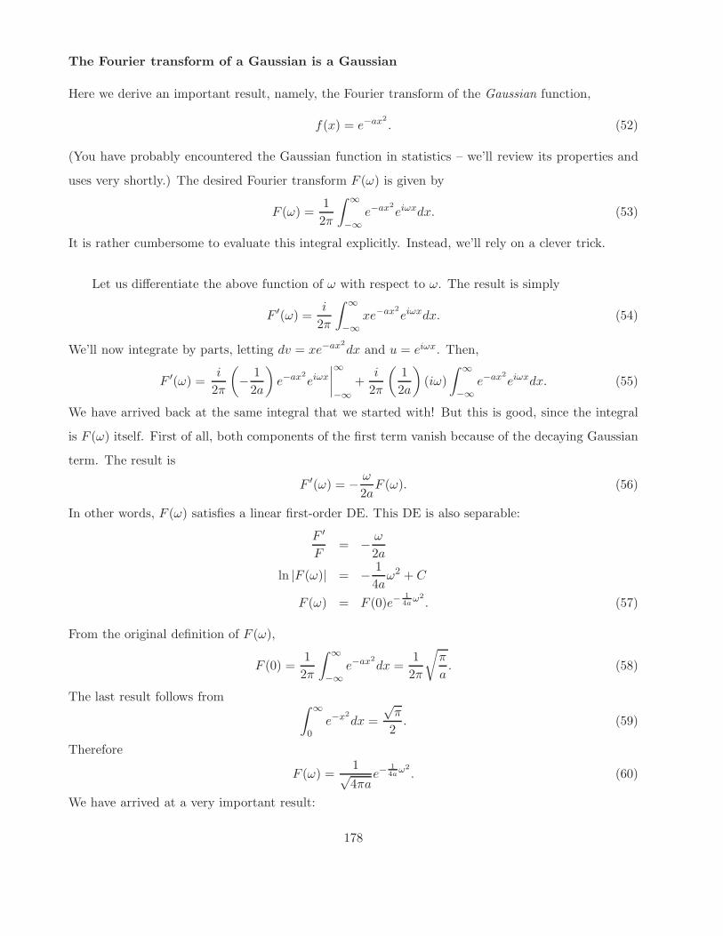
The Fourier transform of a Gaussian is a Gaussian

Here we derive an important result, namely, the Fourier transform of the Gaussian function,

f(x) = e−ax2

. (52)

(You have probably encountered the Gaussian function in statistics – we’ll review its properties and

uses very shortly.) The desired Fourier transform F (ω) is given by

F (ω) =1

2π

∫

∞

−∞

e−ax2

eiωxdx. (53)

It is rather cumbersome to evaluate this integral explicitly. Instead, we’ll rely on a clever trick.

Let us differentiate the above function of ω with respect to ω. The result is simply

F ′(ω) =i

2π

∫

∞

−∞

xe−ax2

eiωxdx. (54)

We’ll now integrate by parts, letting dv = xe−ax2

dx and u = eiωx. Then,

F ′(ω) =i

2π

(

− 1

2a

)

e−ax2

eiωx

∣

∣

∣

∣

∞

−∞

+i

2π

(

1

2a

)

(iω)

∫

∞

−∞

e−ax2

eiωxdx. (55)

We have arrived back at the same integral that we started with! But this is good, since the integral

is F (ω) itself. First of all, both components of the first term vanish because of the decaying Gaussian

term. The result is

F ′(ω) = − ω

2aF (ω). (56)

In other words, F (ω) satisfies a linear first-order DE. This DE is also separable:

F ′

F= − ω

2a

ln |F (ω)| = − 1

4aω2 + C

F (ω) = F (0)e−1

4aω2

. (57)

From the original definition of F (ω),

F (0) =1

2π

∫

∞

−∞

e−ax2

dx =1

2π

√

π

a. (58)

The last result follows from∫

∞

0e−x2

dx =

√π

2. (59)

Therefore

F (ω) =1√4πa

e−1

4aω2

. (60)

We have arrived at a very important result:

178

The Fourier transform of the Gaussian function (in x), f(x) = e−ax2

,

is the Gaussian function (in ω), F (ω) =1√4πa

e−1

4aω2

.

Now let us make the following change of constants:

b =1

4a, → a =

1

4b. (61)

Then

F (ω) =1√4πa

e−1

4aω2 →

√

b

πe−bω2

f(x) = e−ax2 → e−1

4bx2

. (62)

If we now multiply both results by

√

π

b, we arrive at the result:

F (ω) = e−bω2 → f(x) =

√

π

be−

1

4bx2

. (63)

The inverse Fourier transform of the simple Gaussian e−bω2

is the function

√

π

be−

1

4bx2

.

We’ll use this result in the next lecture.

179

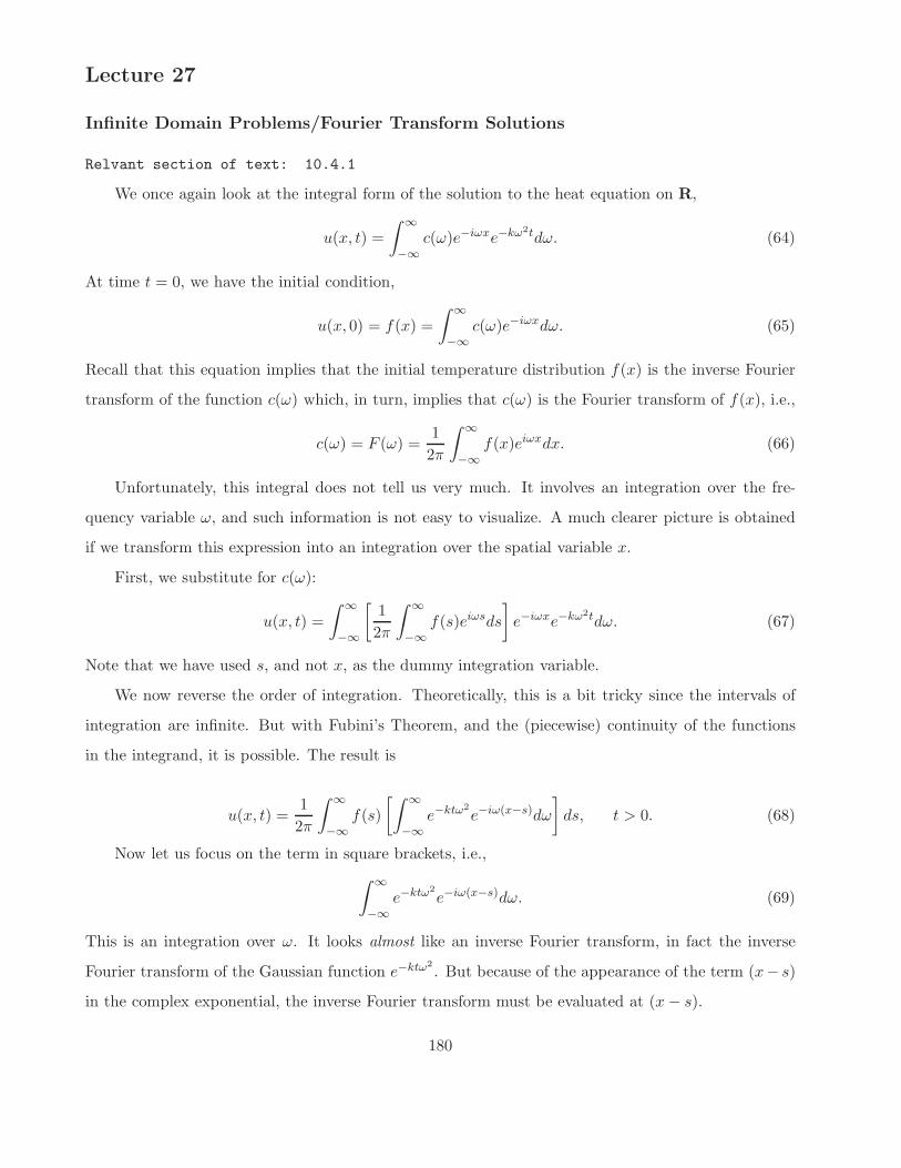
Lecture 27

Infinite Domain Problems/Fourier Transform Solutions

Relvant section of text: 10.4.1

We once again look at the integral form of the solution to the heat equation on R,

u(x, t) =

∫

∞

−∞

c(ω)e−iωxe−kω2tdω. (64)

At time t = 0, we have the initial condition,

u(x, 0) = f(x) =

∫

∞

−∞

c(ω)e−iωxdω. (65)

Recall that this equation implies that the initial temperature distribution f(x) is the inverse Fourier

transform of the function c(ω) which, in turn, implies that c(ω) is the Fourier transform of f(x), i.e.,

c(ω) = F (ω) =1

2π

∫

∞

−∞

f(x)eiωxdx. (66)

Unfortunately, this integral does not tell us very much. It involves an integration over the fre-

quency variable ω, and such information is not easy to visualize. A much clearer picture is obtained

if we transform this expression into an integration over the spatial variable x.

First, we substitute for c(ω):

u(x, t) =

∫

∞

−∞

[

1

2π

∫

∞

−∞

f(s)eiωsds

]

e−iωxe−kω2tdω. (67)

Note that we have used s, and not x, as the dummy integration variable.

We now reverse the order of integration. Theoretically, this is a bit tricky since the intervals of

integration are infinite. But with Fubini’s Theorem, and the (piecewise) continuity of the functions

in the integrand, it is possible. The result is

u(x, t) =1

2π

∫

∞

−∞

f(s)

[∫

∞

−∞

e−ktω2

e−iω(x−s)dω

]

ds, t > 0. (68)

Now let us focus on the term in square brackets, i.e.,

∫

∞

−∞

e−ktω2

e−iω(x−s)dω. (69)

This is an integration over ω. It looks almost like an inverse Fourier transform, in fact the inverse

Fourier transform of the Gaussian function e−ktω2

. But because of the appearance of the term (x− s)

in the complex exponential, the inverse Fourier transform must be evaluated at (x − s).

180

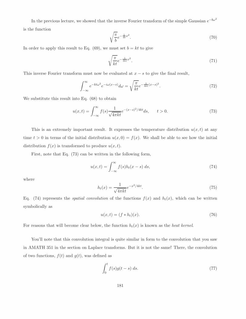
In the previous lecture, we showed that the inverse Fourier transform of the simple Gaussian e−bω2

is the function√

π

be−

1

4bx2

. (70)

In order to apply this result to Eq. (69), we must set b = kt to give

√

π

kte−

1

4ktx2

. (71)

This inverse Fourier transform must now be evaluated at x − s to give the final result,

∫

∞

−∞

e−ktω2

e−iω(x−s)dω =

√

π

kte−

1

4kt(x−s)2 . (72)

We substitute this result into Eq. (68) to obtain

u(x, t) =

∫

∞

−∞

f(s)1√

4πkte−(x−s)2/4ktds, t > 0. (73)

This is an extremely important result. It expresses the temperature distribution u(x, t) at any

time t > 0 in terms of the initial distribution u(x, 0) = f(x). We shall be able to see how the initial

distribution f(x) is transformed to produce u(x, t).

First, note that Eq. (73) can be written in the following form,

u(x, t) =

∫

∞

−∞

f(s)ht(x − s) ds, (74)

where

ht(x) =1√

4πkte−x2/4kt. (75)

Eq. (74) represents the spatial convolution of the functions f(x) and ht(x), which can be written

symbolically as

u(x, t) = (f ∗ ht)(x). (76)

For reasons that will become clear below, the function ht(x) is known as the heat kernel.

You’ll note that this convolution integral is quite similar in form to the convolution that you saw

in AMATH 351 in the section on Laplace transforms. But it is not the same! There, the convolution

of two functions, f(t) and g(t), was defined as

∫ t

0f(s)g(t − s) ds. (77)

181

Note that the integration starts at s = 0 (the initial time) and terminates at t. The spatial convolution

involves integration over the entire real line R = (−∞,∞).

Before we get to the actual convolution in Eq. (74), let us examine the function ht(x). You’ve

seen something like this function before – the infamous Gaussian or normal distribution function from

statistics:

N(x0, σ, x) =1√

2πσ2e−(x−x0)2/2σ2

. (78)

You may recall that x0 signifies the mean of the distribution and σ its standard deviation. The quantity

σ2 is the variance of the distribution. The function N(x0, σ, x) achieves a maximum value at x = x0.

Of course, it is the shifted version of the normal distribution with mean 0:

N(0, σ, x) =1√

2πσ2e−x2/2σ2

. (79)

First of all, the normal distribution is normalized, i.e.,

∫

∞

−∞

N(x0, σ, x) dx = 1, σ > 0. (80)

As a distribution function, we may define the expectation value of a function f(x) as follows:

E[f(x)] =

∫

∞

−∞

f(x)N(x0, σ, x) dx. (81)

The expectation value of x, or the mean of the distribution N is

E[x] =

∫

∞

−∞

xN(x0, σ, x) dx = x0. (82)

The variance of the distribution is the expectation value of (x − x0)2:

E[(x − x0)2] =

∫

∞

−∞

(x − x0)2N(x0, σ, x) dx = σ2. (83)

This implies that the expectation value of x2 is (Exercise)

E[x2] = σ2 + x20. (84)

The standard deviation σ is a measure of the “width” of the normal distribution. At x = x0 ± σ,

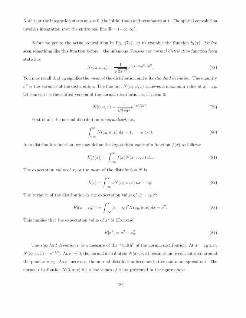
N(x0, σ, x) = e−1/2. As σ → 0, the normal distribution N(x0, σ, x) becomes more concentrated around

the point x = x0. As σ increases, the normal distribution becomes flatter and more spread out. The

normal distribution N(0, σ, x) for a few values of σ are presented in the figure above.

182

0

0.5

1

1.5

2

-3 -2 -1 0 1 2 3

G(t)

t

Gaussian functions

sigma = 1

sigma = 0.5

sigma = 0.25

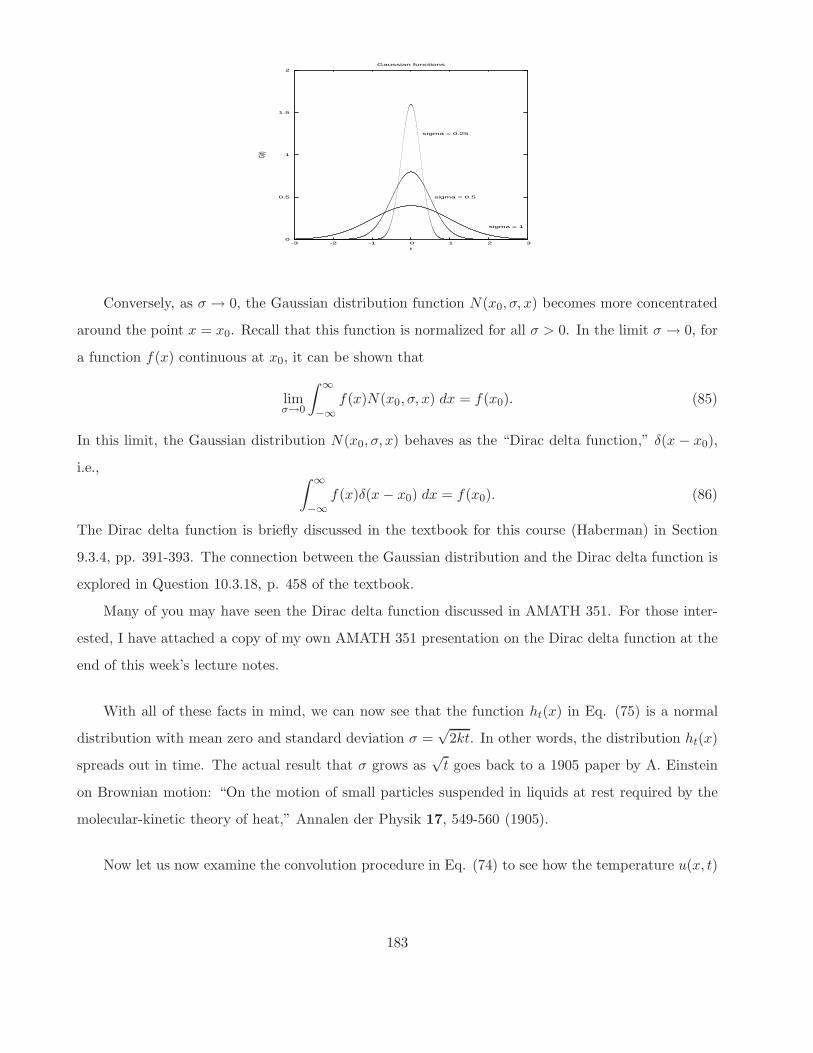
Conversely, as σ → 0, the Gaussian distribution function N(x0, σ, x) becomes more concentrated

around the point x = x0. Recall that this function is normalized for all σ > 0. In the limit σ → 0, for

a function f(x) continuous at x0, it can be shown that

limσ→0

∫

∞

−∞

f(x)N(x0, σ, x) dx = f(x0). (85)

In this limit, the Gaussian distribution N(x0, σ, x) behaves as the “Dirac delta function,” δ(x − x0),

i.e.,∫

∞

−∞

f(x)δ(x − x0) dx = f(x0). (86)

The Dirac delta function is briefly discussed in the textbook for this course (Haberman) in Section

9.3.4, pp. 391-393. The connection between the Gaussian distribution and the Dirac delta function is

explored in Question 10.3.18, p. 458 of the textbook.

Many of you may have seen the Dirac delta function discussed in AMATH 351. For those inter-

ested, I have attached a copy of my own AMATH 351 presentation on the Dirac delta function at the

end of this week’s lecture notes.

With all of these facts in mind, we can now see that the function ht(x) in Eq. (75) is a normal

distribution with mean zero and standard deviation σ =√

2kt. In other words, the distribution ht(x)

spreads out in time. The actual result that σ grows as√

t goes back to a 1905 paper by A. Einstein

on Brownian motion: “On the motion of small particles suspended in liquids at rest required by the

molecular-kinetic theory of heat,” Annalen der Physik 17, 549-560 (1905).

Now let us now examine the convolution procedure in Eq. (74) to see how the temperature u(x, t)

183

is produced from the initial data function f(x). For convenience, we write the equation again,

u(x, t) =

∫

∞

−∞

f(s)ht(x − s) ds. (87)

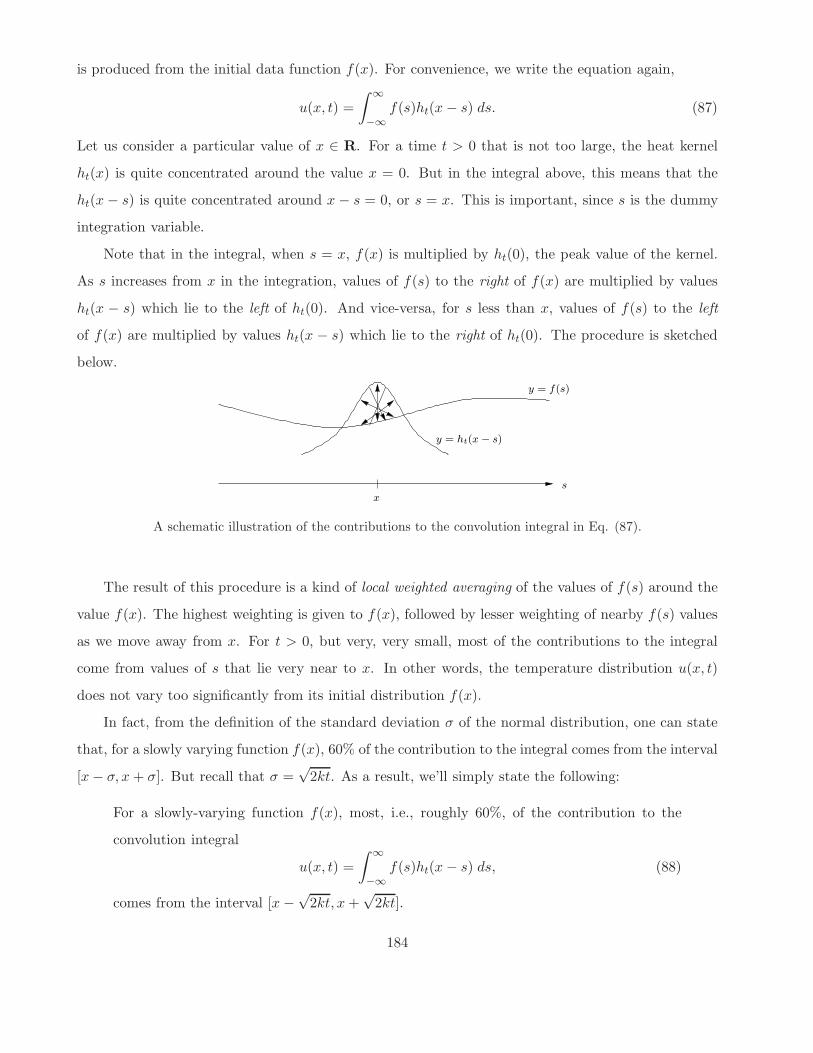
Let us consider a particular value of x ∈ R. For a time t > 0 that is not too large, the heat kernel

ht(x) is quite concentrated around the value x = 0. But in the integral above, this means that the

ht(x − s) is quite concentrated around x − s = 0, or s = x. This is important, since s is the dummy

integration variable.

Note that in the integral, when s = x, f(x) is multiplied by ht(0), the peak value of the kernel.

As s increases from x in the integration, values of f(s) to the right of f(x) are multiplied by values

ht(x − s) which lie to the left of ht(0). And vice-versa, for s less than x, values of f(s) to the left

of f(x) are multiplied by values ht(x − s) which lie to the right of ht(0). The procedure is sketched

below.

y = ht(x − s)

x

y = f(s)

s

A schematic illustration of the contributions to the convolution integral in Eq. (87).

The result of this procedure is a kind of local weighted averaging of the values of f(s) around the

value f(x). The highest weighting is given to f(x), followed by lesser weighting of nearby f(s) values

as we move away from x. For t > 0, but very, very small, most of the contributions to the integral

come from values of s that lie very near to x. In other words, the temperature distribution u(x, t)

does not vary too significantly from its initial distribution f(x).

In fact, from the definition of the standard deviation σ of the normal distribution, one can state

that, for a slowly varying function f(x), 60% of the contribution to the integral comes from the interval

[x − σ, x + σ]. But recall that σ =√

2kt. As a result, we’ll simply state the following:

For a slowly-varying function f(x), most, i.e., roughly 60%, of the contribution to the

convolution integral

u(x, t) =

∫

∞

−∞

f(s)ht(x − s) ds, (88)

comes from the interval [x −√

2kt, x +√

2kt].

184

Of course, as t increases, this interval gets wider and wider, meaning that we we must average

f(s) over a larger interval - actually, always we perform the averaging over the entire real line, but the

most significant contributions are over the interval mentioned above. The widening of this interval

as t → ∞ essentially accounts for the “smoothing” of the temperature distribution function (or the

chemical concentration in the diffusion equation) as t increases.

Let us now consider the special case where the initial temperature distribution f(x) is concentrated

at a point, namely,

f(x) = Aδ(x − x0). (89)

This would imply that the total thermal energy at time t = 0 in the infinite rod is

cρ

∫

∞

−∞

f(x) dx = cρ

∫

∞

−∞

Aδ(x − x0) dx = cρA. (90)

(Recall that k = K/(cρ).)

For t > 0, the temperature function u(x, t) is given by

u(x, t) =

∫

∞

−∞

f(s)ht(x − s) ds

=

∫

∞

−∞

Aδ(x − x0)ht(x − s) ds

= Aht(x − x0), (91)

where we have used the fact that the only contribution to the integral comes from the point at which

the argument of the Dirac delta function is zero, namely, x0. Thus,

u(x, t) = Aht(x − x0) =A√4πkt

e−(x−x0)2/4kt. (92)

A temperature distribution f(x) that is initially concentrated at a point x0 evolves as a Gaussian

distribution of mean x = 0 and standard deviation√

2kt. The total area under this distribution is

always A.

185

Appendix: Supplementary material on the “Dirac delta function”

(from ERV’s lecture notes on AMATH 351, in the section on ‘‘Laplace Transforms’’)

Those unfamiliar with Laplace transforms (or those simply wishing to get to the main result) can

skip the following section and proceed to the section entitled “Dirac delta function”.

A motivating example

Suppose you have a chemical (or radioactive, for that matter) species “X” in a beaker that decays

according to the rate lawdx

dt= −kx. (93)

where x(t) is the concentration at time t. Suppose that at time t = 0, there is x0 amount of X present.

Of course, if the beaker is left alone, then the amount of X at time t ≥ 0 will be given by

x(t) = x0e−kt. (94)

Now suppose that at time a > 0, you quickly (i.e., instantaneously) add an amount A > 0 of X to the

beaker. Then what is x(t), the amount of X at time t ≥ 0?

Well, for 0 ≤ t < a, i.e., for all times before you add A units of X to the beaker, x(t) is given by

Eq. (94) above. Then at t = a, there would have been x0e−ka in the beaker, but you added A, to give

x(a) = x0e−ka + A. Then starting at t = a, the system will evolve according to the rate law. We can

consider x(a) as the initial condition and measure time from t = a. The amount of X in the beaker

will be

x(t) = (x0e−ka + A)e−k(t−a), for t ≥ a. (95)

Let’s summarize our result compactly: For the above experiment, the amount of X in the beaker will

be given by

x(t) =

x0e−kt, 0 ≤ t < a,

x0e−kt + Ae−k(t−a), t ≥ a.

(96)

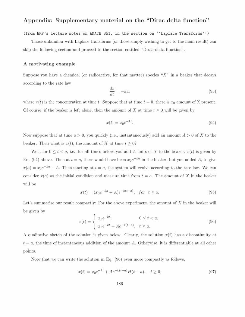
A qualitative sketch of the solution is given below. Clearly, the solution x(t) has a discontinuity at

t = a, the time of instantaneous addition of the amount A. Otherwise, it is differentiable at all other

points.

Note that we can write the solution in Eq. (96) even more compactly as follows,

x(t) = x0e−kt + Ae−k(t−a)H(t − a), t ≥ 0, (97)

186

x(a) + A

0 a t

x(t) vs. t

x(a)

x0

A

where H(t) is the Heaviside function reviewed earlier. We shall return to this solution a little later.

We now ask whether the above operation – the instantaneous addition of an amount A of X to

the beaker – can be represented mathematically, perhaps with a function f(t) so that the evolution of

x(t) can be expressed asdx

dt= −kx + f(t), (98)

where f(t) models the instantaneous addition of an amount A of X at time t = a. The answer is

“Yes,” and f(t) will be the so-called “Dirac delta function” f(t) = Aδ(t − a).

But in order to appreciate this result, let us now consider the case of a less brutal addition of X

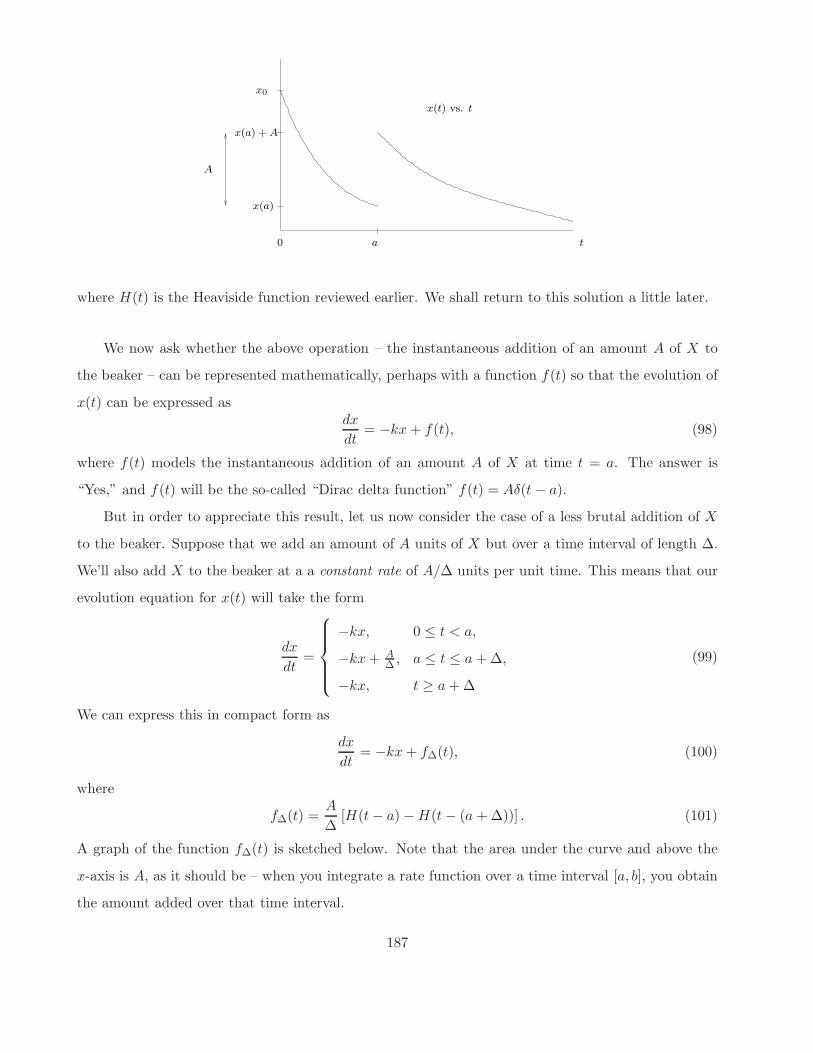
to the beaker. Suppose that we add an amount of A units of X but over a time interval of length ∆.

We’ll also add X to the beaker at a a constant rate of A/∆ units per unit time. This means that our

evolution equation for x(t) will take the form

dx

dt=

−kx, 0 ≤ t < a,

−kx + A∆ , a ≤ t ≤ a + ∆,

−kx, t ≥ a + ∆

(99)

We can express this in compact form as

dx

dt= −kx + f∆(t), (100)

where

f∆(t) =A

∆[H(t − a) − H(t − (a + ∆))] . (101)

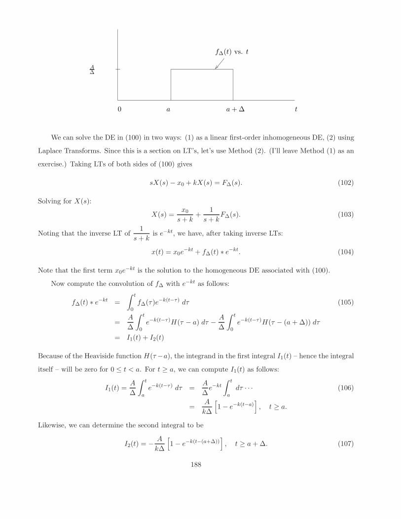
A graph of the function f∆(t) is sketched below. Note that the area under the curve and above the

x-axis is A, as it should be – when you integrate a rate function over a time interval [a, b], you obtain

the amount added over that time interval.

187

A∆

0 ta + ∆a

f∆(t) vs. t

We can solve the DE in (100) in two ways: (1) as a linear first-order inhomogeneous DE, (2) using

Laplace Transforms. Since this is a section on LT’s, let’s use Method (2). (I’ll leave Method (1) as an

exercise.) Taking LTs of both sides of (100) gives

sX(s) − x0 + kX(s) = F∆(s). (102)

Solving for X(s):

X(s) =x0

s + k+

1

s + kF∆(s). (103)

Noting that the inverse LT of1

s + kis e−kt, we have, after taking inverse LTs:

x(t) = x0e−kt + f∆(t) ∗ e−kt. (104)

Note that the first term x0e−kt is the solution to the homogeneous DE associated with (100).

Now compute the convolution of f∆ with e−kt as follows:

f∆(t) ∗ e−kt =

∫ t

0f∆(τ)e−k(t−τ) dτ (105)

=A

∆

∫ t

0e−k(t−τ)H(τ − a) dτ − A

∆

∫ t

0e−k(t−τ)H(τ − (a + ∆)) dτ

= I1(t) + I2(t)

Because of the Heaviside function H(τ −a), the integrand in the first integral I1(t) – hence the integral

itself – will be zero for 0 ≤ t < a. For t ≥ a, we can compute I1(t) as follows:

I1(t) =A

∆

∫ t

ae−k(t−τ) dτ =

A

∆e−kt

∫ t

adτ · · · (106)

=A

k∆

[

1 − e−k(t−a)]

, t ≥ a.

Likewise, we can determine the second integral to be

I2(t) = − A

k∆

[

1 − e−k(t−(a+∆))]

, t ≥ a + ∆. (107)

188

The final result for x(t) is

x(t) = x0e−kt + I1(t)H(t − a) + I2(t)H(t − (a + ∆)). (108)

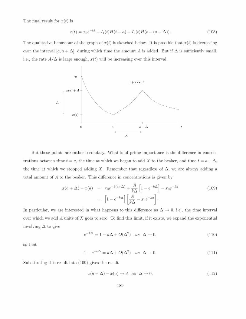
The qualitative behaviour of the graph of x(t) is sketched below. It is possible that x(t) is decreasing

over the interval [a, a + ∆], during which time the amount A is added. But if ∆ is sufficiently small,

i.e., the rate A/∆ is large enough, x(t) will be increasing over this interval.

∆

0 a t

x(t) vs. t

x(a)

x0

A

x(a) + A

a + ∆

But these points are rather secondary. What is of prime importance is the difference in concen-

trations between time t = a, the time at which we began to add X to the beaker, and time t = a+ ∆,

the time at which we stopped adding X. Remember that regardless of ∆, we are always adding a

total amount of A to the beaker. This difference in concentrations is given by

x(a + ∆) − x(a) = x0e−k(a+∆) +

A

k∆

[

1 − e−k∆]

− x0e−ka (109)

=[

1 − e−k∆]

[

A

k∆− x0e

−ka

]

.

In particular, we are interested in what happens to this difference as ∆ → 0, i.e., the time interval

over which we add A units of X goes to zero. To find this limit, if it exists, we expand the exponential

involving ∆ to give

e−k∆ = 1 − k∆ + O(∆2) as ∆ → 0, (110)

so that

1 − e−k∆ = k∆ + O(∆2) as ∆ → 0. (111)

Substituting this result into (109) gives the result

x(a + ∆) − x(a) → A as ∆ → 0. (112)

189

In other words, in the limit ∆ → 0, the graph of x(t) will exhibit a discontinuity at t = a. The

magnitude of this “jump” is A, precisely was found with the earlier method.

We now return to the inhomogeneous DE in (100) and examine the behaviour of the inhomoge-

neous term f∆(t) as ∆ → 0. Recall that this is the “driving” term, the function that models the

addition of a total of A units of X to the beaker over the time interval [a, a + ∆]. The width of the

box that makes up the graph of f∆(t) is ∆. The height of the box isA

∆. In this way, the area of the

box – the total amount of X delivered – is A. As ∆ decreases, the box gets thinner and higher. In the

limit ∆ → 0, we have produced a function f0(t) that is zero everywhere except at t = a, where it is

undefined. This is the idea behind the “Dirac delta function,” which we explore in more detail below.

The Dirac delta function

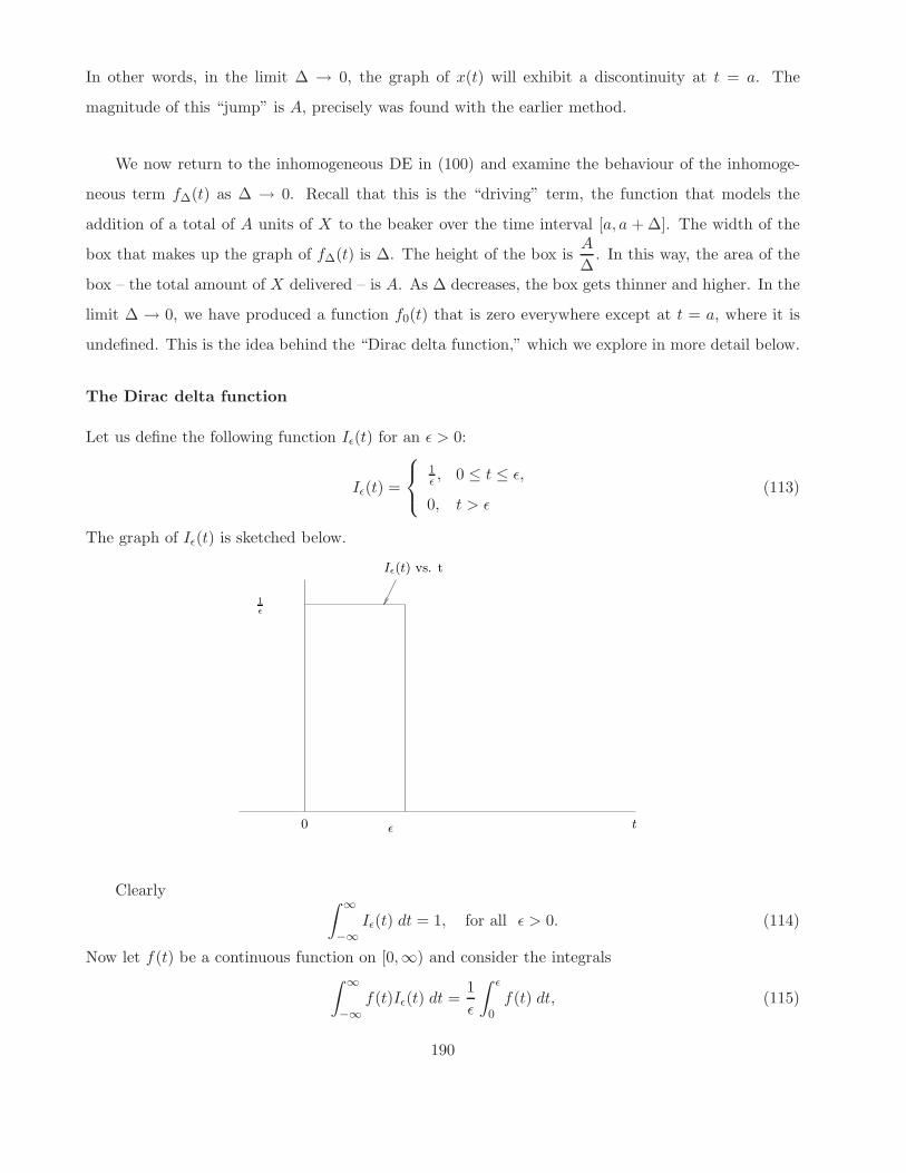
Let us define the following function Iǫ(t) for an ǫ > 0:

Iǫ(t) =

1ǫ , 0 ≤ t ≤ ǫ,

0, t > ǫ(113)

The graph of Iǫ(t) is sketched below.

1

ǫ

0 ǫ t

Iǫ(t) vs. t

Clearly∫

∞

−∞

Iǫ(t) dt = 1, for all ǫ > 0. (114)

Now let f(t) be a continuous function on [0,∞) and consider the integrals∫

∞

−∞

f(t)Iǫ(t) dt =1

ǫ

∫ ǫ

0f(t) dt, (115)

190

in particular for small ǫ and limit ǫ → 0. For any ǫ > 0, because of the continuity of f(t), there exists,

by the Mean Value Theorem for Integrals, a cǫ ∈ [0, ǫ] such that

∫ ǫ

0f(t) dt = f(cǫ) · ǫ. (116)

Therefore,∫ ǫ

0f(t)Iǫ(t) dt = f(cǫ). (117)

As ǫ → 0, cǫ → 0 since the interval [0, ǫ] → {0}. Therefore

limǫ→0

∫ ǫ

0f(t)Iǫ(t) dt = f(0). (118)

We may, of course, translate the function Iǫ(t) to produce the result

limǫ→0

∫

∞

−∞

f(t)Iǫ(t − a) dt = f(a). (119)

This is essentially a definition of the “Dirac delta function,” which is not a function but rather

a “generalized function” that is defined in terms of integrals over continuous functions. In proper

mathematical parlance, the Dirac delta function is a distribution. The Dirac delta function δ(t) is

defined by the integral∫

∞

−∞

f(t)δ(t) dt. (120)

Moreover∫ d

cf(t)δ(t) dt = 0, if c > 0. (121)

As well, we have the translation result

∫

∞

−∞

f(t)δ(t − a) dt = f(a). (122)

Finally, we compute the Laplace transform of the Dirac delta function. In this case f(t) = e−st

so that

L[δ(t − a)] =

∫

∞

0e−stδ(t − a) dt = e−as, a ≥ 0. (123)

Let us now return to the substance X problem examined earlier where an amount A of substance

X is added to a beaker over a time interval of length ∆. Comparing the function f∆(t) used for that

problem and the function Iǫ(t) defined above, we see that ∆ = ǫ and

f∆(t) = AI∆(t). (124)

191

From our discussion above on the Dirac delta function, in the limit ∆ → 0 the function f∆(t) becomes

f(t) = Aδ(t − a). (125)

Therefore, the differential equation for x(t) modelling the instantaneous addition of A to the beaker

is given bydx

dt= −kx + Aδ(t − a). (126)

We now compute x(t) using the result in Eq. (104) obtained from Laplace transforms. Using f(t) =

Aδ(t − a), the convolution in this equation becomes

(g ∗ f)(t) = e−kt ∗ Aδ(t − a) (127)

= A

∫ t

0e−k(t−τ)δ(τ − a) dτ

The above integral is zero for 0 ≤ t < a. For t ≥ a, this integral is nonzero and becomes

A

∫ t

0e−k(t−τ)δ(τ − a) dτ = Ae−k(t−a), t ≥ a. (128)

Therefore, the solution x(t) becomes

x(t) = x0e−kt + Ae−k(t−a)H(t − a), (129)

in agreement with the result obtained in Eq. (97).

There are alternate ways to construct the Dirac delta function. For example, one could make the

function Iǫ(t) symmetric about the point 0 by defining it as follows:

Iǫ(t) =

1ǫ , − ǫ

2 ≤ t ≤ ǫ2 ,

0, |t| > ǫ2

(130)

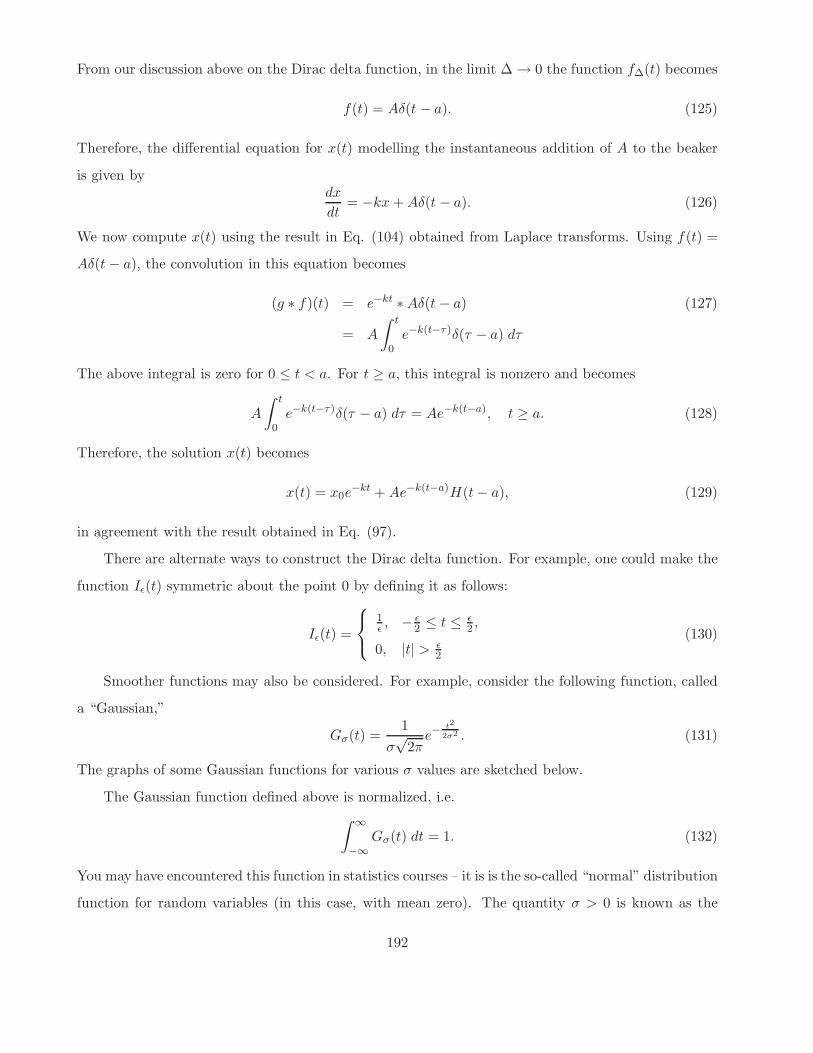
Smoother functions may also be considered. For example, consider the following function, called

a “Gaussian,”

Gσ(t) =1

σ√

2πe−

t2

2σ2 . (131)

The graphs of some Gaussian functions for various σ values are sketched below.

The Gaussian function defined above is normalized, i.e.

∫

∞

−∞

Gσ(t) dt = 1. (132)

You may have encountered this function in statistics courses – it is is the so-called “normal” distribution

function for random variables (in this case, with mean zero). The quantity σ > 0 is known as the

192

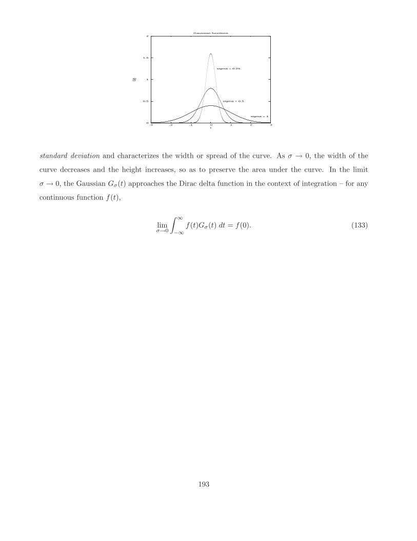
0

0.5

1

1.5

2

-3 -2 -1 0 1 2 3

G(t)

t

Gaussian functions

sigma = 1

sigma = 0.5

sigma = 0.25

standard deviation and characterizes the width or spread of the curve. As σ → 0, the width of the

curve decreases and the height increases, so as to preserve the area under the curve. In the limit

σ → 0, the Gaussian Gσ(t) approaches the Dirac delta function in the context of integration – for any

continuous function f(t),

limσ→0

∫

∞

−∞

f(t)Gσ(t) dt = f(0). (133)

193