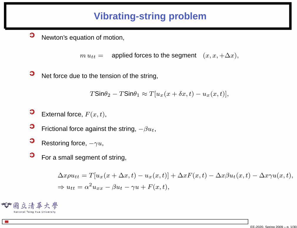
Vibrating-string problem

Newton’s equation of motion,

mutt = applied forces to the segment (x, x,+∆x),

Net force due to the tension of the string,

TSinθ2 − TSinθ1 ≈ T [ux(x+ δx, t) − ux(x, t)],

External force, F (x, t),

Frictional force against the string, −βut,

Restoring force, −γu,

For a small segment of string,

∆xρutt = T [ux(x+ ∆x, t) − ux(x, t)] + ∆xF (x, t) − ∆xβut(x, t) − ∆xγu(x, t),

⇒ utt = α2uxx − βut − γu+ F (x, t),

EE-2020, Spring 2009 – p. 1/30

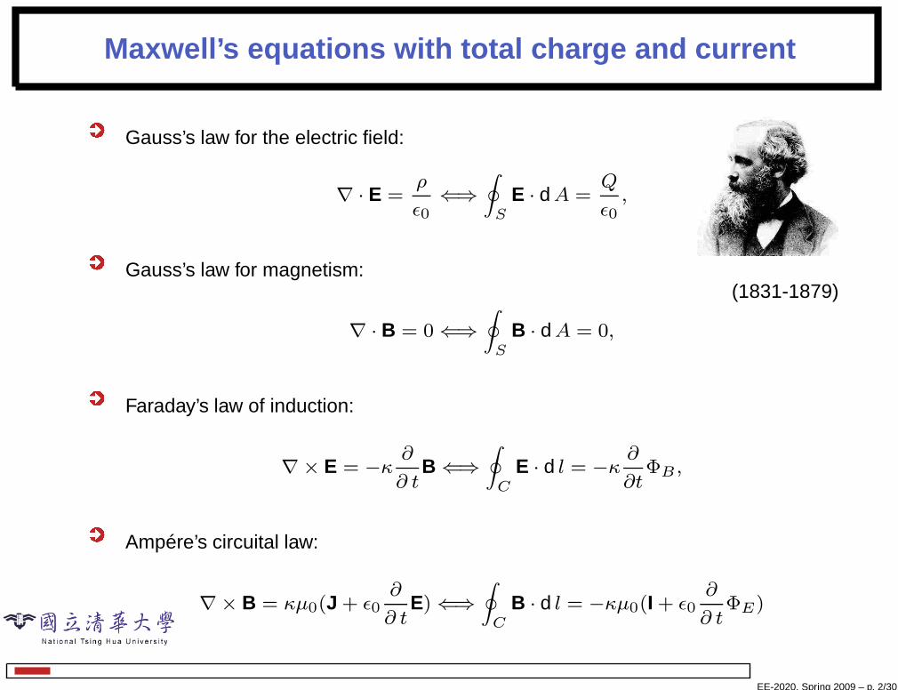
Maxwell’s equations with total charge and current

(1831-1879)

Gauss’s law for the electric field:

∇ · E =ρ

ǫ0⇐⇒

∮

S

E · dA =Q

ǫ0,

Gauss’s law for magnetism:

∇ · B = 0 ⇐⇒

∮

S

B · dA = 0,

Faraday’s law of induction:

∇× E = −κ∂

∂ tB ⇐⇒

∮

C

E · d l = −κ∂

∂tΦB ,

Ampére’s circuital law:

∇× B = κµ0(J + ǫ0∂

∂ tE) ⇐⇒

∮

C

B · d l = −κµ0(I + ǫ0∂

∂ tΦE)

EE-2020, Spring 2009 – p. 2/30

Helmholtz wave equations

For a source-free medium, ρ = J = 0,

∇× (∇× E) = −µ0ǫ0∂2

∂ t2E,

⇒ ∇(∇ · E) −∇2E = −µ0ǫ0∂2

∂ t2E.

When ∇ · E = 0, one has wave equation,

∇2E = µ0ǫ0∂2

∂ t2E

which has following expression of the solutions, in 1D,

E = x̂[f+(z − vt) + f−(z + vt)],

with v2 = 1µ0ǫ0

= c2.

plane wave solutions: E+ = E0 cos(kz − ωt), where ωk

= c.

EE-2020, Spring 2009 – p. 3/30

Wave equation

The wave equation contains a second-order time derivative, utt, it requires two

initial conditions

u(x, t = 0) = f(x), and ut(x, t = 0) = g(x),

For electric current along the wire, with the Kirchhoff’s laws,

ix + C vt +Gv = 0,

vx + L it +R i = 0,

The transmission-line equations

ixx = CL itt + (CR+GL) it +GR i,

vxx = CLvtt + (CR+GL) vt +GRv,

If G = R = 0, and α2 = 1/CL,

itt = α2, ixx,

vtt = α2 vxx.

EE-2020, Spring 2009 – p. 4/30

The D’Alembert solution of the wave equation

For the diffusion problems (the parabolic case), we solve the bounded case(0 ≤ x ≤ L) by separation of variables while solve the unbounded case(−∞ < x < ∞) by the Fourier transform.

For the wave problems (the hyperbolic case), we will do the opposite .

PDE: utt = α2uxx, −∞ < x < ∞, 0 < t <∞

ICs:

u(x, 0) = f(x)

ut(x, 0) = g(x), −∞ < x < ∞

Replace (x, t) by new canonical coordinates (ξ, η), i.e. the moving-coordinate,

ξ = x+ α t η = x− α t

the PDE becomes

uξη = 0

with the solution of arbitrary functions of ξ or η, i.e.

u(ξ, η) = φ(η) + ψ(ξ),

EE-2020, Spring 2009 – p. 5/30

The D’Alembert solution of the wave equation, cont.

In the original coordinates x and t, we have

u(x, t) = Φ(x− α t) + Ψ(x+ α t),

this is the general solution of the wave equation.

Physically it represents the sum of any two moving waves, each moving in oppositedirection with the velocity α. Eg.

u(x, t) = Sin(x− α t), (one right-moving wave)

u(x, t) = (x+ α t)2, (one left-moving wave)

u(x, t) = Sin(x− α t) + (x+ α t)2, (two oppositely moving waves)

EE-2020, Spring 2009 – p. 6/30

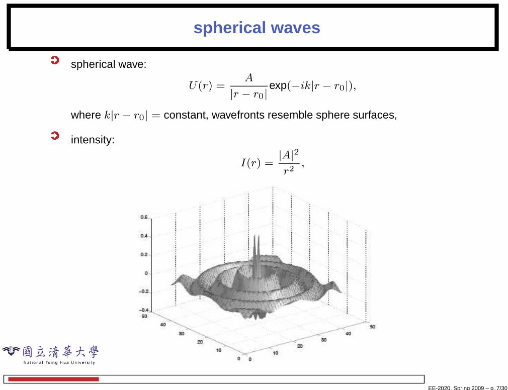
spherical waves

spherical wave:

U(r) =A

|r − r0|exp(−ik|r − r0|),

where k|r − r0| = constant, wavefronts resemble sphere surfaces,

intensity:

I(r) =|A|2

r2,

EE-2020, Spring 2009 – p. 7/30

ICs

Substitute the general solution into the two ICs,

ICs:

u(x, 0) = f(x)

ut(x, 0) = g(x), −∞ < x < ∞

for arbitrary functions φ and ψ, we have

φ(x) + ψ(x) = f(x),

−αφ′(x) + αψ′(x) = g(x),

then by integrating from x0 to x,

−αφ(x) + αψ(x) =

∫ x

x0

g(ξ)d ξ +K

where K is an integration constant.

EE-2020, Spring 2009 – p. 8/30

D’Alembert solution

The solutions for φ and ψ are

φ(x) =1

2f(x) −

1

2α

∫ x

x0

g(ξ)d ξ,

ψ(x) =1

2f(x) +

1

2α

∫ x

x0

g(ξ)d ξ,

The D’Alembert solution,

u(x, t) =1

2[f(x− α, t) + f(x+ α t)] +

1

2α

∫ x+α t

x−α t

g(ξ)d ξ.

EE-2020, Spring 2009 – p. 9/30

Examples of the D’Alembert solution

1. Motion of an initial Sine wave,

PDE: utt = α2uxx, −∞ < x < ∞, 0 < t <∞

ICs:

u(x, 0) = Sin(x)

ut(x, 0) = 0, −∞ < x <∞

The solution

u(x, t) =1

2[Sin(x− α t) + Sin(x+ α t)].

2. Initial velocity given

ICs:

u(x, 0) = 0

ut(x, 0) = Sin(x), −∞ < x < ∞

The solution

u(x, t) =1

2α

∫ x+α t

x−α t

Sin(ξ)d ξ =1

2α[Cos(x+ α t) − Cos(x− α t)].

EE-2020, Spring 2009 – p. 10/30

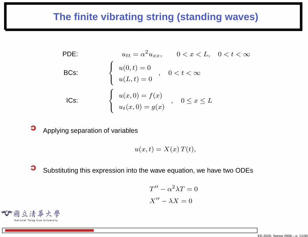
The finite vibrating string (standing waves)

PDE: utt = α2uxx, 0 < x < L, 0 < t <∞

BCs:

u(0, t) = 0

u(L, t) = 0, 0 < t <∞

ICs:

u(x, 0) = f(x)

ut(x, 0) = g(x), 0 ≤ x ≤ L

Applying separation of variables

u(x, t) = X(x)T (t),

Substituting this expression into the wave equation, we have two ODEs

T ′′ − α2λT = 0

X′′ − λX = 0

EE-2020, Spring 2009 – p. 11/30

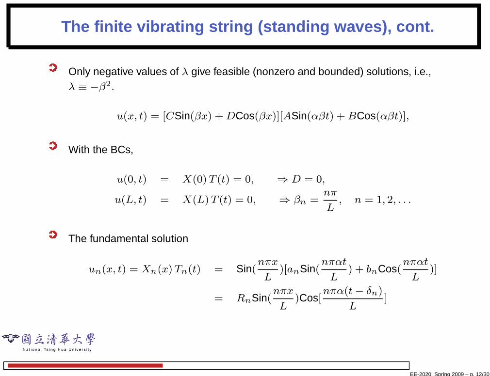
The finite vibrating string (standing waves), cont.

Only negative values of λ give feasible (nonzero and bounded) solutions, i.e.,λ ≡ −β2.

u(x, t) = [CSin(βx) +DCos(βx)][ASin(αβt) +BCos(αβt)],

With the BCs,

u(0, t) = X(0)T (t) = 0, ⇒ D = 0,

u(L, t) = X(L)T (t) = 0, ⇒ βn =nπ

L, n = 1, 2, . . .

The fundamental solution

un(x, t) = Xn(x)Tn(t) = Sin(nπx

L)[anSin(

nπαt

L) + bnCos(

nπαt

L)]

= RnSin(nπx

L)Cos[

nπα(t− δn)

L]

EE-2020, Spring 2009 – p. 12/30

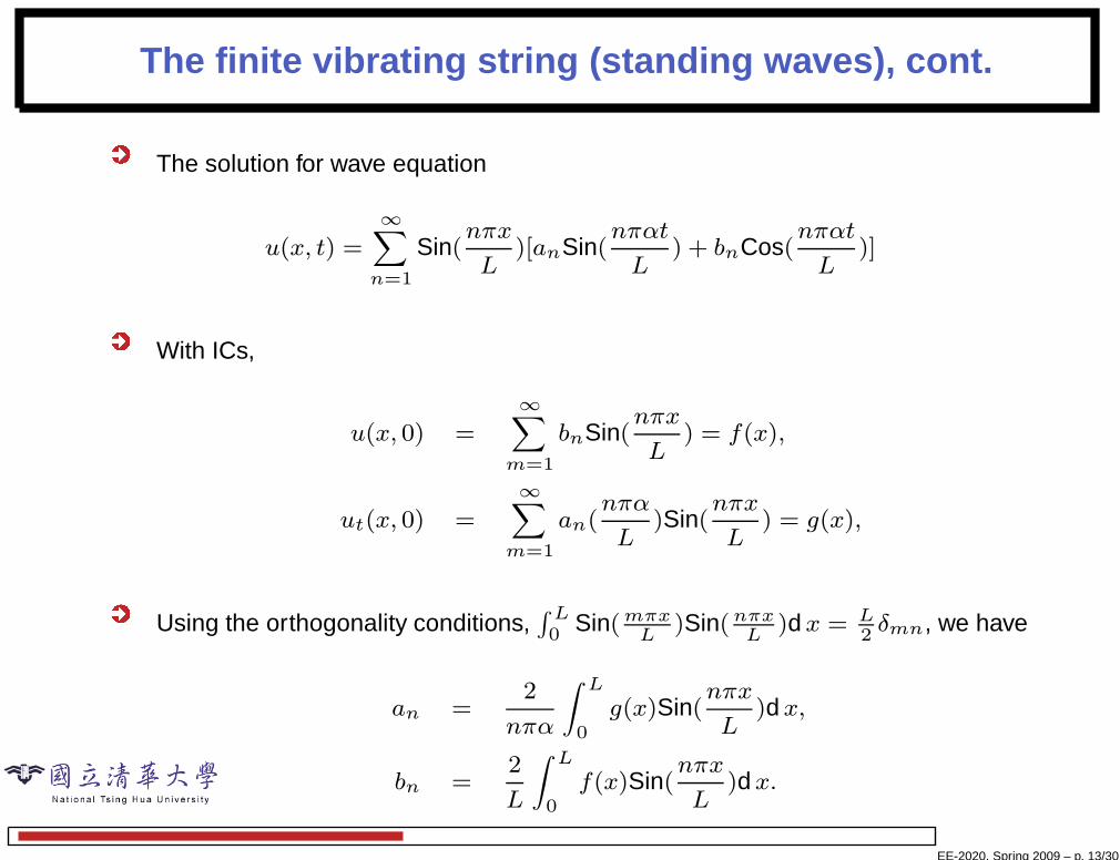
The finite vibrating string (standing waves), cont.

The solution for wave equation

u(x, t) =∞∑

n=1

Sin(nπx

L)[anSin(

nπαt

L) + bnCos(

nπαt

L)]

With ICs,

u(x, 0) =∞∑

m=1

bnSin(nπx

L) = f(x),

ut(x, 0) =∞∑

m=1

an(nπα

L)Sin(

nπx

L) = g(x),

Using the orthogonality conditions,∫ L

0 Sin( mπxL

)Sin( nπxL

)dx = L2δmn, we have

an =2

nπα

∫ L

0g(x)Sin(

nπx

L)dx,

bn =2

L

∫ L

0f(x)Sin(

nπx

L)dx.

EE-2020, Spring 2009 – p. 13/30

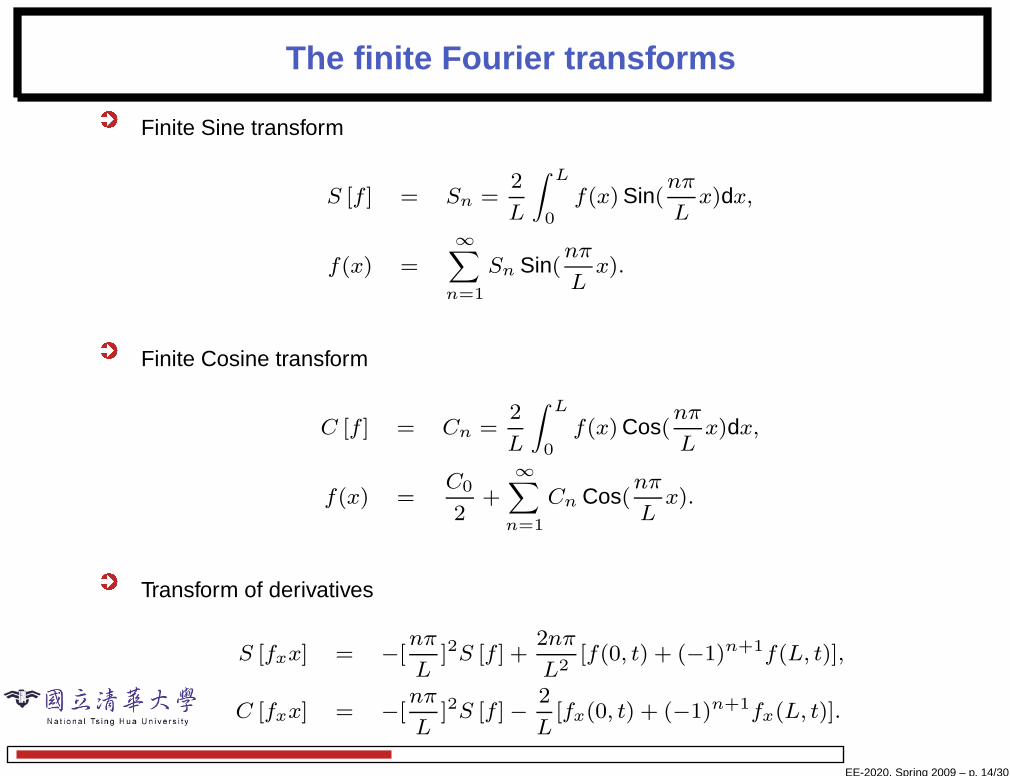
The finite Fourier transforms

Finite Sine transform

S [f ] = Sn =2

L

∫ L

0f(x) Sin(

nπ

Lx)dx,

f(x) =

∞∑

n=1

Sn Sin(nπ

Lx).

Finite Cosine transform

C [f ] = Cn =2

L

∫ L

0f(x) Cos(

nπ

Lx)dx,

f(x) =C0

2+

∞∑

n=1

Cn Cos(nπ

Lx).

Transform of derivatives

S [fxx] = −[nπ

L]2S [f ] +

2nπ

L2[f(0, t) + (−1)n+1f(L, t)],

C [fxx] = −[nπ

L]2S [f ] −

2

L[fx(0, t) + (−1)n+1fx(L, t)].

EE-2020, Spring 2009 – p. 14/30

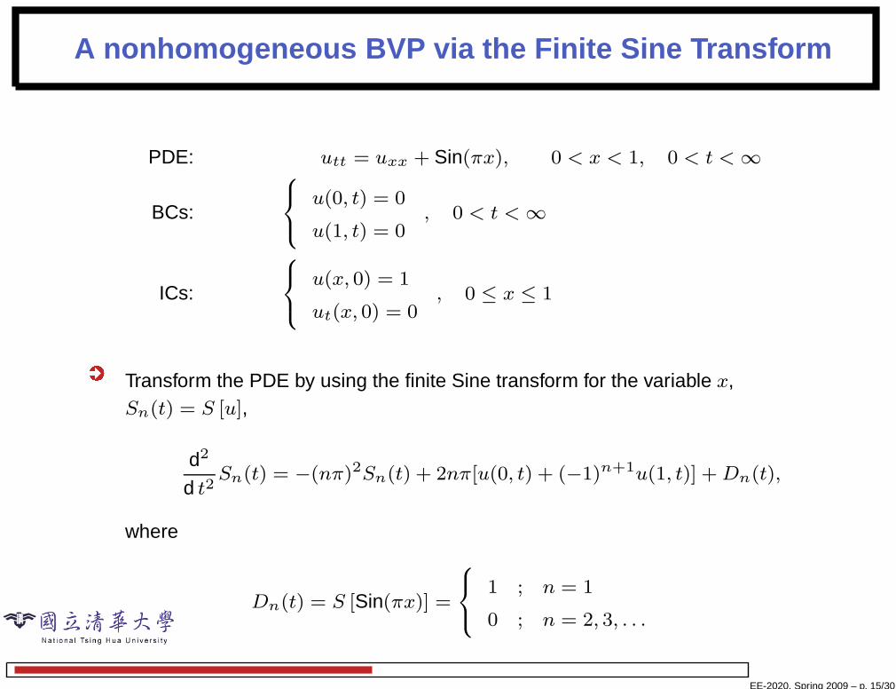
A nonhomogeneous BVP via the Finite Sine Transform

PDE: utt = uxx + Sin(πx), 0 < x < 1, 0 < t < ∞

BCs:

u(0, t) = 0

u(1, t) = 0, 0 < t <∞

ICs:

u(x, 0) = 1

ut(x, 0) = 0, 0 ≤ x ≤ 1

Transform the PDE by using the finite Sine transform for the variable x,Sn(t) = S [u],

d2

d t2Sn(t) = −(nπ)2Sn(t) + 2nπ[u(0, t) + (−1)n+1u(1, t)] +Dn(t),

where

Dn(t) = S [Sin(πx)] =

1 ; n = 1

0 ; n = 2, 3, . . .

EE-2020, Spring 2009 – p. 15/30

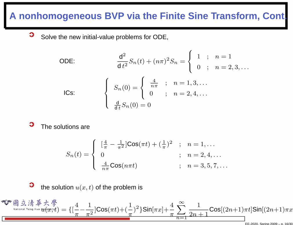
A nonhomogeneous BVP via the Finite Sine Transform, Cont.

Solve the new initial-value problems for ODE,

ODE:d2

d t2Sn(t) + (nπ)2Sn =

1 ; n = 1

0 ; n = 2, 3, . . .

ICs:

Sn(0) =

4nπ

; n = 1, 3, . . .

0 ; n = 2, 4, . . .

dd tSn(0) = 0

The solutions are

Sn(t) =

[ 4π− 1

π2]Cos(πt) + ( 1

π)2 ; n = 1, . . .

0 ; n = 2, 4, . . .

4nπ

Cos(nπt) ; n = 3, 5, 7, . . .

the solution u(x, t) of the problem is

u(x, t) = {[4

π−

1

π2]Cos(πt)+(

1

π)2}Sin[πx]+

4

π

∞∑

n=1

1

2n+ 1Cos[(2n+1)πt]Sin[(2n+1)πx].

EE-2020, Spring 2009 – p. 16/30

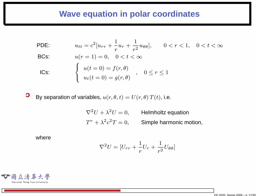
Wave equation in polar coordinates

PDE: utt = c2[urr +1

rur +

1

r2uθθ], 0 < r < 1, 0 < t < ∞

BCs: u(r = 1) = 0, 0 < t <∞

ICs:

u(t = 0) = f(r, θ)

ut(t = 0) = g(r, θ), 0 ≤ r ≤ 1

By separation of variables, u(r, θ, t) = U(r, θ)T (t), i.e.

∇2U + λ2U = 0, Helmholtz equation

T” + λ2c2T = 0, Simple harmonic motion,

where

∇2U = [Urr +1

rUr +

1

r2Uθθ]

EE-2020, Spring 2009 – p. 17/30

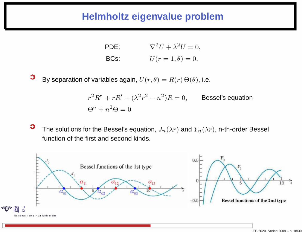
Helmholtz eigenvalue problem

PDE: ∇2U + λ2U = 0,

BCs: U(r = 1, θ) = 0,

By separation of variables again, U(r, θ) = R(r)Θ(θ), i.e.

r2R” + rR′ + (λ2r2 − n2)R = 0, Bessel’s equation

Θ” + n2Θ = 0

The solutions for the Bessel’s equation, Jn(λr) and Yn(λr), n-th-order Besselfunction of the first and second kinds.

EE-2020, Spring 2009 – p. 18/30

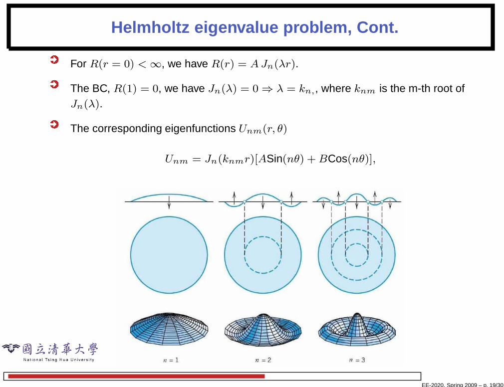
Helmholtz eigenvalue problem, Cont.

For R(r = 0) <∞, we have R(r) = AJn(λr).

The BC, R(1) = 0, we have Jn(λ) = 0 ⇒ λ = kn,, where knm is the m-th root ofJn(λ).

The corresponding eigenfunctions Unm(r, θ)

Unm = Jn(knmr)[ASin(nθ) +BCos(nθ)],

EE-2020, Spring 2009 – p. 19/30

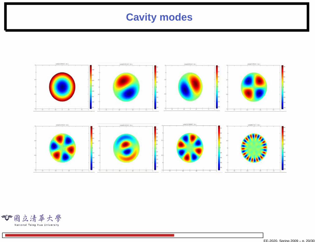
Cavity modes

EE-2020, Spring 2009 – p. 20/30

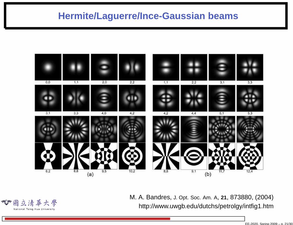
Hermite/Laguerre/Ince-Gaussian beams

M. A. Bandres, J. Opt. Soc. Am. A, 21, 873880, (2004)http://www.uwgb.edu/dutchs/petrolgy/intfig1.htm

EE-2020, Spring 2009 – p. 21/30

Helmholtz eigenvalue problem, Cont.

For the time equation, we have

T” + k2nmc

2T = 0, Simple harmonic motion,

⇒ Tnm(t) = ASin(knmct) + BCos(knmct).

The total solution of our problem is

u(r, θ, t) =

∞∑

n=0

∞∑

m=1

Jn(knmr)Cos(nθ)[AnmSin(knmct) +BnmCos(knmct)]

EE-2020, Spring 2009 – p. 22/30

Wave equation in polar coordinates, θ-independent

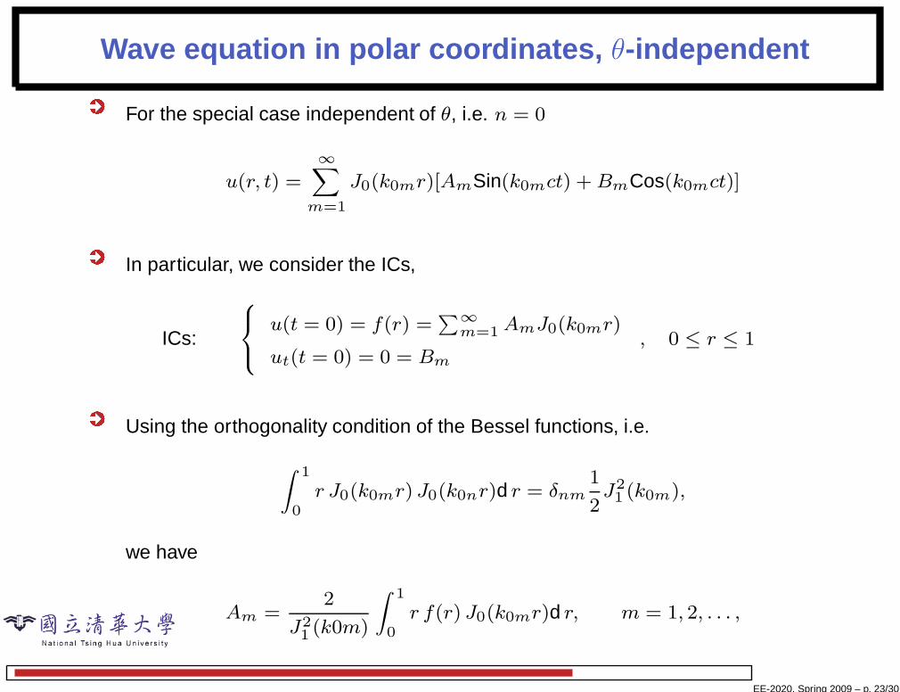
For the special case independent of θ, i.e. n = 0

u(r, t) =∞∑

m=1

J0(k0mr)[AmSin(k0mct) +BmCos(k0mct)]

In particular, we consider the ICs,

ICs:

u(t = 0) = f(r) =∑

∞

m=1AmJ0(k0mr)

ut(t = 0) = 0 = Bm

, 0 ≤ r ≤ 1

Using the orthogonality condition of the Bessel functions, i.e.

∫ 1

0r J0(k0mr) J0(k0nr)d r = δnm

1

2J21 (k0m),

we have

Am =2

J21 (k0m)

∫ 1

0r f(r) J0(k0mr)d r, m = 1, 2, . . . ,

EE-2020, Spring 2009 – p. 23/30

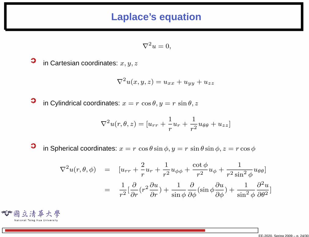
Laplace’s equation

∇2u = 0,

in Cartesian coordinates: x, y, z

∇2u(x, y, z) = uxx + uyy + uzz

in Cylindrical coordinates: x = r cos θ, y = r sin θ, z

∇2u(r, θ, z) = [urr +1

rur +

1

r2uθθ + uzz ]

in Spherical coordinates: x = r cos θ sinφ, y = r sin θ sinφ, z = r cosφ

∇2u(r, θ, φ) = [urr +2

rur +

1

r2uφφ +

cotφ

r2uφ +

1

r2 sin2 φuθθ]

=1

r2[∂

∂r(r2

∂u

∂r) +

1

sinφ

∂

∂φ(sinφ

∂u

∂φ) +

1

sin2 φ

∂2u

∂θ2]

EE-2020, Spring 2009 – p. 24/30

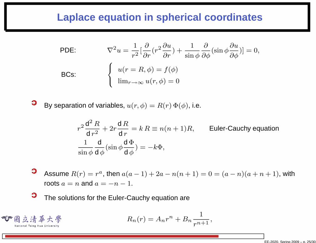
Laplace equation in spherical coordinates

PDE: ∇2u =1

r2[∂

∂r(r2

∂u

∂r) +

1

sinφ

∂

∂φ(sinφ

∂u

∂φ)] = 0,

BCs:

u(r = R,φ) = f(φ)

limr→∞ u(r, φ) = 0

By separation of variables, u(r, φ) = R(r) Φ(φ), i.e.

r2d2R

d r2+ 2r

dRd r

= kR ≡ n(n+ 1)R, Euler-Cauchy equation

1

sinφ

ddφ

(sinφd Φ

dφ) = −kΦ,

Assume R(r) = ra, then a(a− 1) + 2a− n(n+ 1) = 0 = (a− n)(a+ n+ 1), withroots a = n and a = −n− 1.

The solutions for the Euler-Cauchy equation are

Rn(r) = Anrn +Bn

1

rn+1,

EE-2020, Spring 2009 – p. 25/30

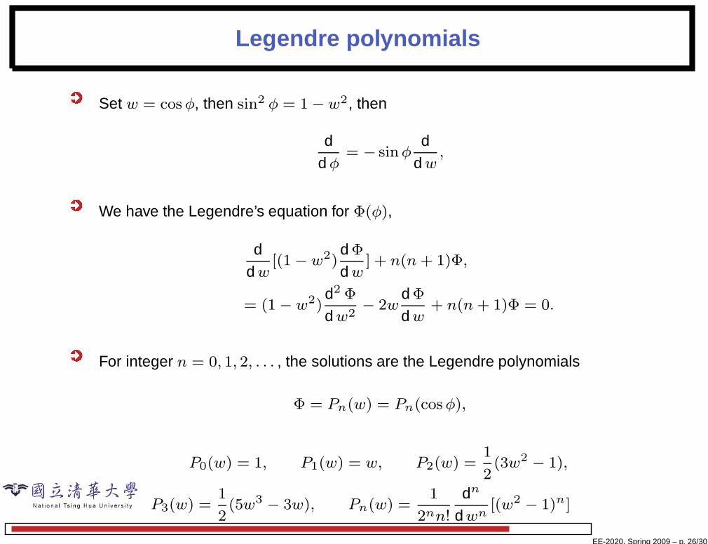
Legendre polynomials

Set w = cosφ, then sin2 φ = 1 − w2, then

ddφ

= − sinφd

dw,

We have the Legendre’s equation for Φ(φ),

ddw

[(1 − w2)d Φ

dw] + n(n+ 1)Φ,

= (1 − w2)d2 Φ

dw2− 2w

d Φ

dw+ n(n+ 1)Φ = 0.

For integer n = 0, 1, 2, . . . , the solutions are the Legendre polynomials

Φ = Pn(w) = Pn(cosφ),

P0(w) = 1, P1(w) = w, P2(w) =1

2(3w2 − 1),

P3(w) =1

2(5w3 − 3w), Pn(w) =

1

2nn!

dn

dwn[(w2 − 1)n]

EE-2020, Spring 2009 – p. 26/30

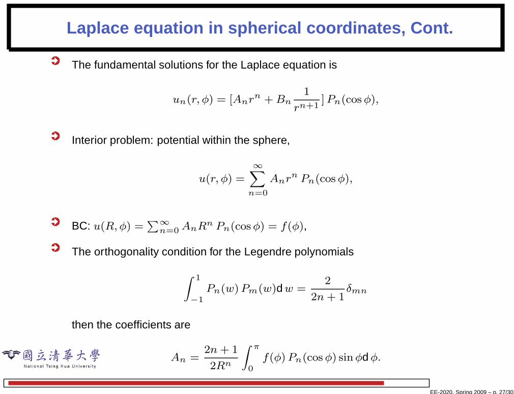
Laplace equation in spherical coordinates, Cont.

The fundamental solutions for the Laplace equation is

un(r, φ) = [Anrn +Bn

1

rn+1]Pn(cosφ),

Interior problem: potential within the sphere,

u(r, φ) =∞∑

n=0

Anrn Pn(cosφ),

BC: u(R,φ) =∑

∞

n=0AnRn Pn(cosφ) = f(φ),

The orthogonality condition for the Legendre polynomials

∫ 1

−1Pn(w)Pm(w)dw =

2

2n+ 1δmn

then the coefficients are

An =2n+ 1

2Rn

∫ π

0f(φ)Pn(cosφ) sinφdφ.

EE-2020, Spring 2009 – p. 27/30

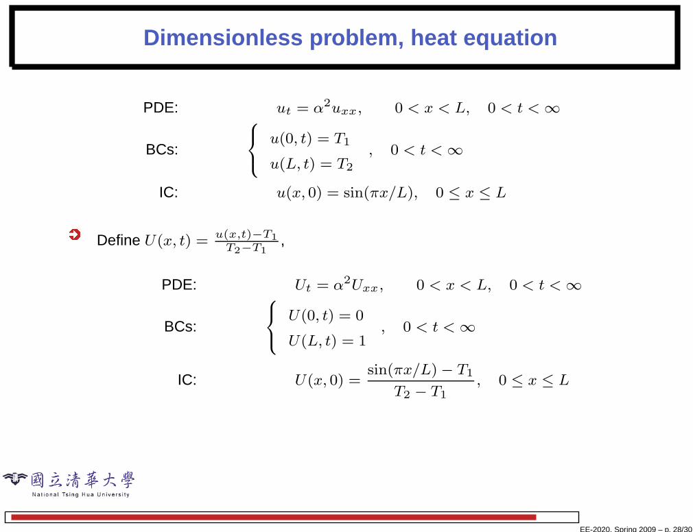
Dimensionless problem, heat equation

PDE: ut = α2uxx, 0 < x < L, 0 < t < ∞

BCs:

u(0, t) = T1

u(L, t) = T2

, 0 < t < ∞

IC: u(x, 0) = sin(πx/L), 0 ≤ x ≤ L

Define U(x, t) =u(x,t)−T1

T2−T1,

PDE: Ut = α2Uxx, 0 < x < L, 0 < t < ∞

BCs:

U(0, t) = 0

U(L, t) = 1, 0 < t < ∞

IC: U(x, 0) =sin(πx/L) − T1

T2 − T1, 0 ≤ x ≤ L

EE-2020, Spring 2009 – p. 28/30

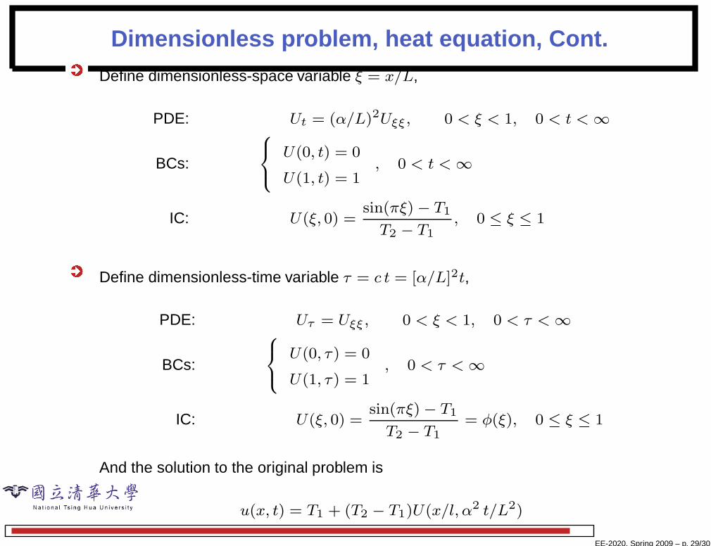
Dimensionless problem, heat equation, Cont.

Define dimensionless-space variable ξ = x/L,

PDE: Ut = (α/L)2Uξξ, 0 < ξ < 1, 0 < t < ∞

BCs:

U(0, t) = 0

U(1, t) = 1, 0 < t < ∞

IC: U(ξ, 0) =sin(πξ) − T1

T2 − T1, 0 ≤ ξ ≤ 1

Define dimensionless-time variable τ = c t = [α/L]2t,

PDE: Uτ = Uξξ, 0 < ξ < 1, 0 < τ < ∞

BCs:

U(0, τ) = 0

U(1, τ) = 1, 0 < τ <∞

IC: U(ξ, 0) =sin(πξ) − T1

T2 − T1= φ(ξ), 0 ≤ ξ ≤ 1

And the solution to the original problem is

u(x, t) = T1 + (T2 − T1)U(x/l, α2 t/L2)

EE-2020, Spring 2009 – p. 29/30

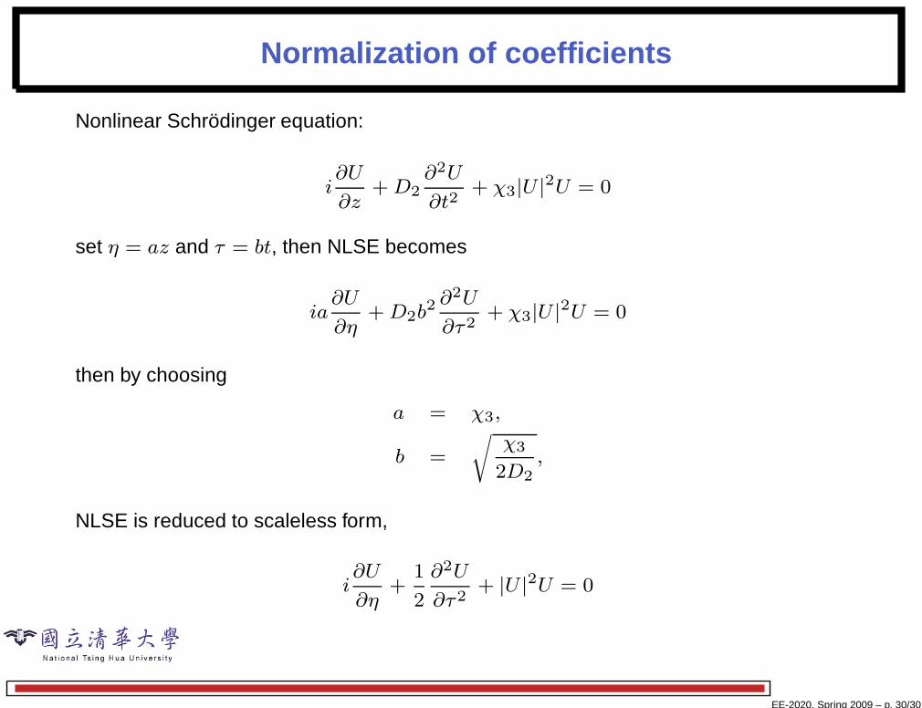
Normalization of coefficients

Nonlinear Schrödinger equation:

i∂U

∂z+D2

∂2U

∂t2+ χ3|U |2U = 0

set η = az and τ = bt, then NLSE becomes

ia∂U

∂η+D2b

2 ∂2U

∂τ2+ χ3|U |2U = 0

then by choosing

a = χ3,

b =

√

χ3

2D2,

NLSE is reduced to scaleless form,

i∂U

∂η+

1

2

∂2U

∂τ2+ |U |2U = 0

EE-2020, Spring 2009 – p. 30/30