Higgs Hunt Using Expert Discriminants in the

ZH→ννbb at the TeVatron

A Senior Honors Thesis

Presented in Partial Fulfillment of the Requirements for graduation

with research distinction in Physics in the undergraduate

colleges of The Ohio State University

by

Douglas Schaefer

The Ohio State University

June 2009

Project Adviser: Professor Brian Winer, Department of Physics

Abstract

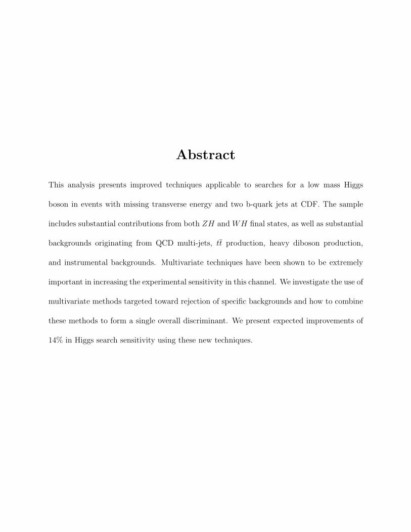
This analysis presents improved techniques applicable to searches for a low mass Higgs

boson in events with missing transverse energy and two b-quark jets at CDF. The sample

includes substantial contributions from both ZH and WH final states, as well as substantial

backgrounds originating from QCD multi-jets, tt production, heavy diboson production,

and instrumental backgrounds. Multivariate techniques have been shown to be extremely

important in increasing the experimental sensitivity in this channel. We investigate the use of

multivariate methods targeted toward rejection of specific backgrounds and how to combine

these methods to form a single overall discriminant. We present expected improvements of

14% in Higgs search sensitivity using these new techniques.

Contents

1 Introduction 1

2 Higgs Mechanism 6

3 The TeVatron and CDF 9

3.1 Collider Detector at Fermilab . . . . . . . . . . . . . . . . . . 10

3.2 Trigger System . . . . . . . . . . . . . . . . . . . . . . . . . . 14

4 Multivariate Techniques 15

4.1 Artificial Neural Networks . . . . . . . . . . . . . . . . . . . . 16

4.2 Boosted Decision Trees (BDT) . . . . . . . . . . . . . . . . . . 16

4.3 Support Vector Machines . . . . . . . . . . . . . . . . . . . . . 18

5 ZH/WH → MET + Jets Analysis 20

5.1 Signals ZH and WH . . . . . . . . . . . . . . . . . . . . . . . 20

i

5.2 Backgrounds . . . . . . . . . . . . . . . . . . . . . . . . . . . . 21

5.2.1 QCD . . . . . . . . . . . . . . . . . . . . . . . . . . . . 21

5.2.2 Electroweak . . . . . . . . . . . . . . . . . . . . . . . . 22

5.2.3 Top . . . . . . . . . . . . . . . . . . . . . . . . . . . . 23

5.2.4 Single Top . . . . . . . . . . . . . . . . . . . . . . . . . 23

5.2.5 Diboson . . . . . . . . . . . . . . . . . . . . . . . . . . 24

5.3 Selection Cuts . . . . . . . . . . . . . . . . . . . . . . . . . . . 25

5.3.1 Kinematic Cuts . . . . . . . . . . . . . . . . . . . . . . 25

5.3.2 b Tagging . . . . . . . . . . . . . . . . . . . . . . . . . 28

5.3.3 Loosening Cuts . . . . . . . . . . . . . . . . . . . . . . 29

6 Expert Multivariate Technique 33

6.1 Track Based Variables - Track MVT . . . . . . . . . . . . . . 33

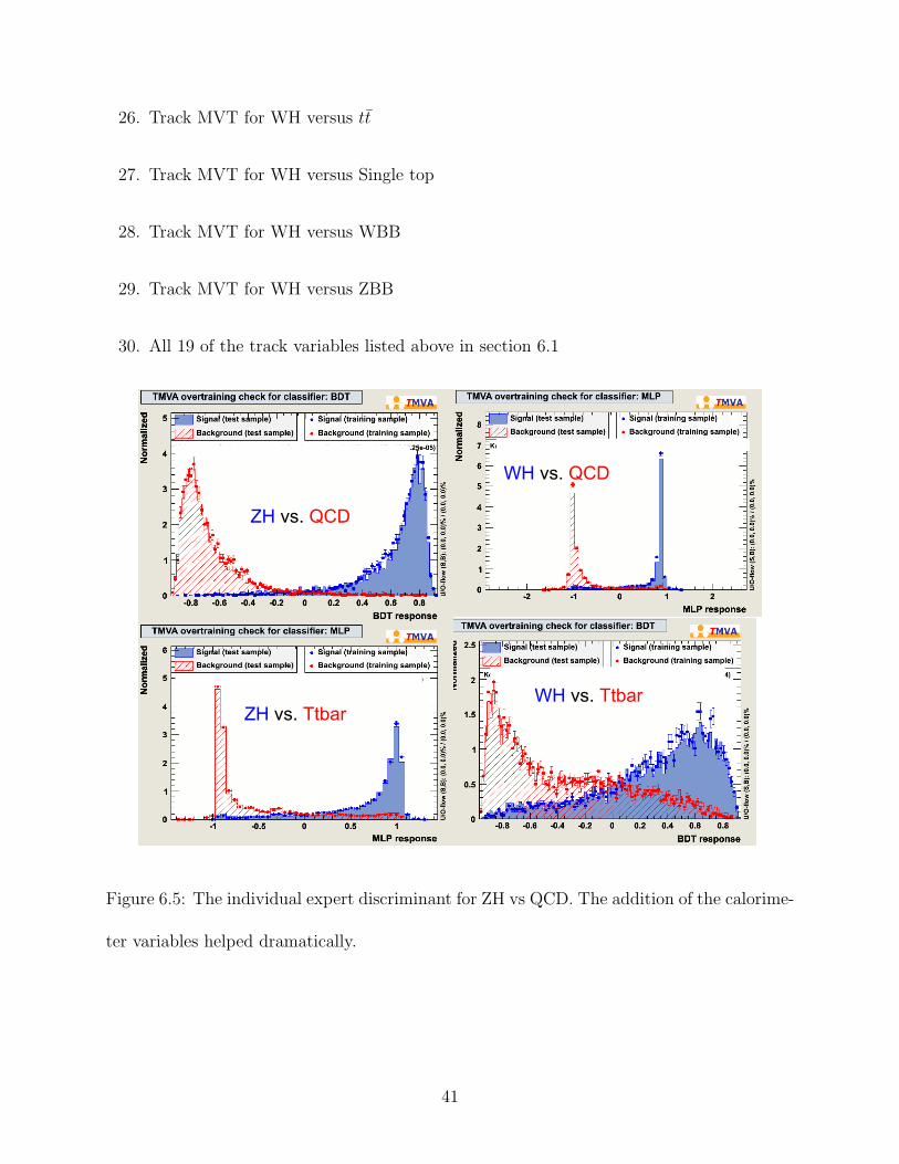
6.2 Individual Expert Discriminants . . . . . . . . . . . . . . . . . 38

6.3 Global Discriminant . . . . . . . . . . . . . . . . . . . . . . . 42

6.4 Control Region Check . . . . . . . . . . . . . . . . . . . . . . 43

7 95% Expected Confidence Level Limits on the Standard Model

Higgs Production 45

ii

7.1 Double SecVtx Tagged Events . . . . . . . . . . . . . . . . . . 46

8 Conclusions 49

iii

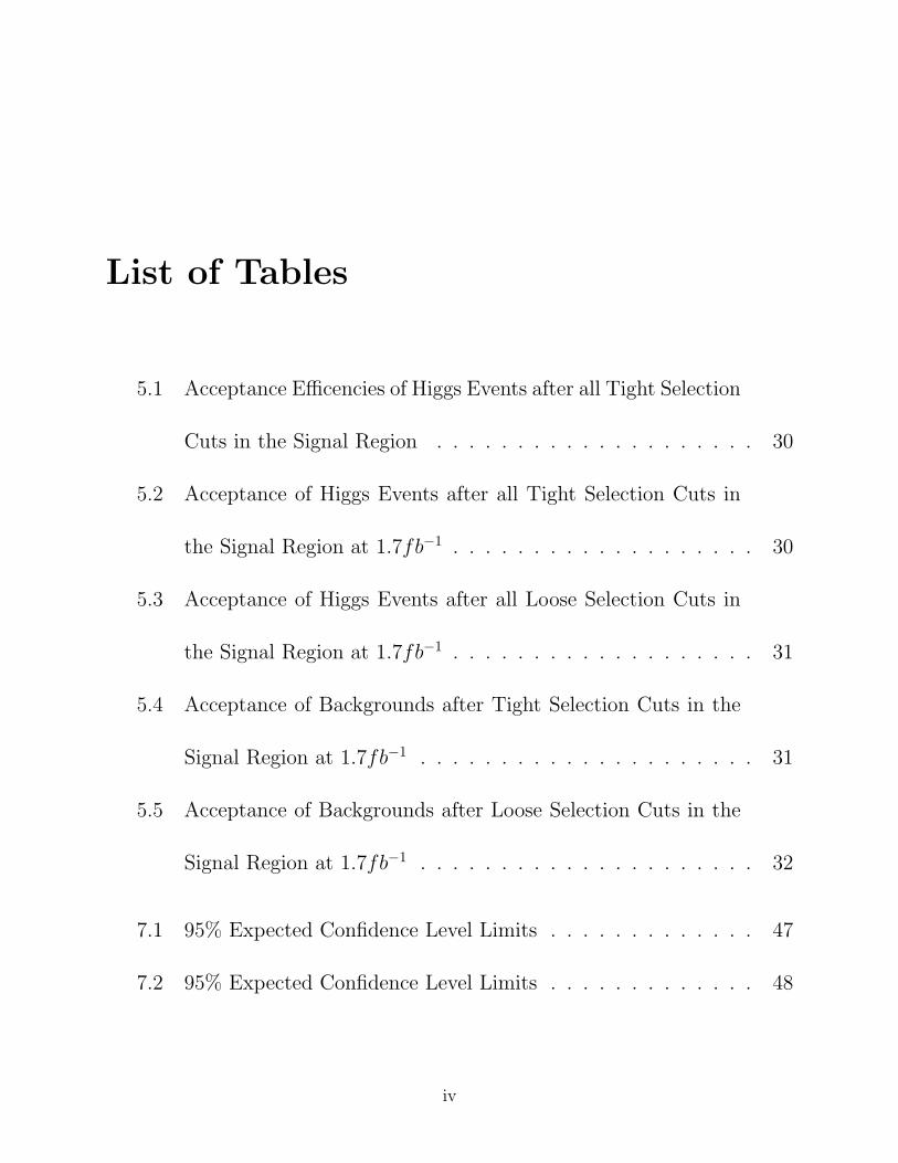
List of Tables

5.1 Acceptance Efficencies of Higgs Events after all Tight Selection

Cuts in the Signal Region . . . . . . . . . . . . . . . . . . . . 30

5.2 Acceptance of Higgs Events after all Tight Selection Cuts in

the Signal Region at 1.7fb−1 . . . . . . . . . . . . . . . . . . . 30

5.3 Acceptance of Higgs Events after all Loose Selection Cuts in

the Signal Region at 1.7fb−1 . . . . . . . . . . . . . . . . . . . 31

5.4 Acceptance of Backgrounds after Tight Selection Cuts in the

Signal Region at 1.7fb−1 . . . . . . . . . . . . . . . . . . . . . 31

5.5 Acceptance of Backgrounds after Loose Selection Cuts in the

Signal Region at 1.7fb−1 . . . . . . . . . . . . . . . . . . . . . 32

7.1 95% Expected Confidence Level Limits . . . . . . . . . . . . . 47

7.2 95% Expected Confidence Level Limits . . . . . . . . . . . . . 48

iv

List of Figures

1.1 An example of the Eightfold Way, which is the meson octet. s

is the strangeness, and q is the charge of the particles. . . . . . 3

1.2 Standard Model of Particle Physics . . . . . . . . . . . . . . . 3

1.3 The Limits that have been placed on the Higgs bosons mass.

The horizontal axis is the mass of the Higgs boson, and the

vertical axis represents the ∆χ2 probability of the Higgs having

a at the given mass. The yellow portions have been ruled out

by experiment. . . . . . . . . . . . . . . . . . . . . . . . . . . 5

2.1 An example of a symmetric potential. . . . . . . . . . . . . . . 8

v

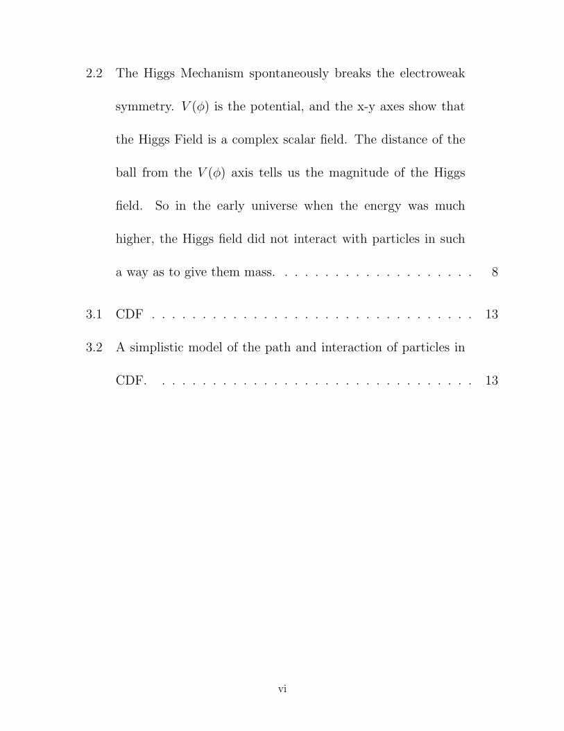
2.2 The Higgs Mechanism spontaneously breaks the electroweak

symmetry. V (φ) is the potential, and the x-y axes show that

the Higgs Field is a complex scalar field. The distance of the

ball from the V (φ) axis tells us the magnitude of the Higgs

field. So in the early universe when the energy was much

higher, the Higgs field did not interact with particles in such

a way as to give them mass. . . . . . . . . . . . . . . . . . . . 8

3.1 CDF . . . . . . . . . . . . . . . . . . . . . . . . . . . . . . . . 13

3.2 A simplistic model of the path and interaction of particles in

CDF. . . . . . . . . . . . . . . . . . . . . . . . . . . . . . . . 13

vi

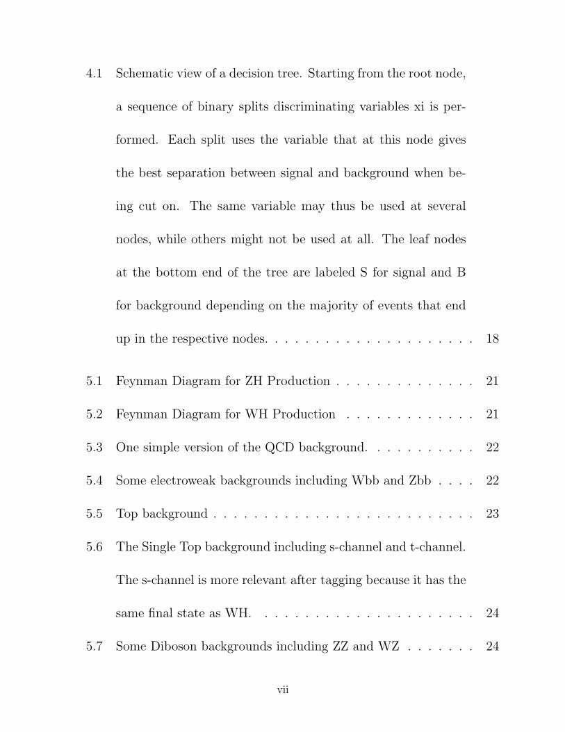
4.1 Schematic view of a decision tree. Starting from the root node,

a sequence of binary splits discriminating variables xi is per-

formed. Each split uses the variable that at this node gives

the best separation between signal and background when be-

ing cut on. The same variable may thus be used at several

nodes, while others might not be used at all. The leaf nodes

at the bottom end of the tree are labeled S for signal and B

for background depending on the majority of events that end

up in the respective nodes. . . . . . . . . . . . . . . . . . . . . 18

5.1 Feynman Diagram for ZH Production . . . . . . . . . . . . . . 21

5.2 Feynman Diagram for WH Production . . . . . . . . . . . . . 21

5.3 One simple version of the QCD background. . . . . . . . . . . 22

5.4 Some electroweak backgrounds including Wbb and Zbb . . . . 22

5.5 Top background . . . . . . . . . . . . . . . . . . . . . . . . . . 23

5.6 The Single Top background including s-channel and t-channel.

The s-channel is more relevant after tagging because it has the

same final state as WH. . . . . . . . . . . . . . . . . . . . . . 24

5.7 Some Diboson backgrounds including ZZ and WZ . . . . . . . 24

vii

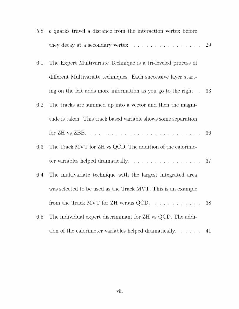
5.8 b quarks travel a distance from the interaction vertex before

they decay at a secondary vertex. . . . . . . . . . . . . . . . . 29

6.1 The Expert Multivariate Technique is a tri-leveled process of

different Multivariate techniques. Each successive layer start-

ing on the left adds more information as you go to the right. . 33

6.2 The tracks are summed up into a vector and then the magni-

tude is taken. This track based variable shows some separation

for ZH vs ZBB. . . . . . . . . . . . . . . . . . . . . . . . . . . 36

6.3 The Track MVT for ZH vs QCD. The addition of the calorime-

ter variables helped dramatically. . . . . . . . . . . . . . . . . 37

6.4 The multivariate technique with the largest integrated area

was selected to be used as the Track MVT. This is an example

from the Track MVT for ZH versus QCD. . . . . . . . . . . . 38

6.5 The individual expert discriminant for ZH vs QCD. The addi-

tion of the calorimeter variables helped dramatically. . . . . . 41

viii

6.6 The Global Discriminating neural network with equal normal-

izations for the signal and background. The signal and back-

ground shapes contain the appropriate mixing of the different

processes. . . . . . . . . . . . . . . . . . . . . . . . . . . . . . 43

6.7 The electroweak control region shows that the Global Expert

Discriminant is well modeled. . . . . . . . . . . . . . . . . . . 44

7.1 The expected shapes for the signal and background in the dou-

ble SecVtx category. . . . . . . . . . . . . . . . . . . . . . . . 47

ix

Chapter 1

Introduction

Since the time of the Greeks, humans have tried to understand the world around them

on a fundamental level. Aristotle theorized that the world was made of four elements: earth,

fire, water, and air. We have come a very long way from these ideas; however, we have

are still interested in the fundamental building blocks of the universe. In 1665, Robert

Hooke made a breakthrough by finding tiny components of matter, which he called cells.

Then came atoms, and slowly we began to see a pattern in the structure of atoms with the

periodic table, which is credited to Dmitri Mendeleev in 1869. The periodic table hinted at

some substructure to atoms.

In 1897, J. J. Thomson discovered the electron through his work with cathode ray tubes,

which changed the notion that atoms were the fundamental building blocks of our universe.

Ernest Rutherford, in 1909, discovered more of the substructure of atoms by shooting alpha

particles or helium nuclei at a thin sheet of gold and looking at the diffraction and reflections

of the alpha particles. Rutherford realized that atoms are mostly empty space. However,

he said that atoms seem to have hard cores, which he called the nucleus. Later came

1

the discovery of the neutron and the proton. All of these particles seemed to make sense,

even the discovery in 1932 of antimatter by Carl Anderson [2] after the prediction of their

existence by Paul Dirac in 1928. Dirac believed in his theory so much that he predicted

a new particle with his theory, and the positron or positively charged electron was born.

However, the discovery, also by Carl Anderson in 1936, of a massive version of the electron,

called a muon, made physicists very worried that all of these particles were not fitting into

some very simple overarching model. There continued to be so many discoveries of new

and interesting particles with no fundamental structure that physicists began to call them

collectively a “particle zoo.” However, this all changed with the introduction of the eightfold

way by Gell-Mann in the 1962. This gave the “particle zoo” some structure and made a

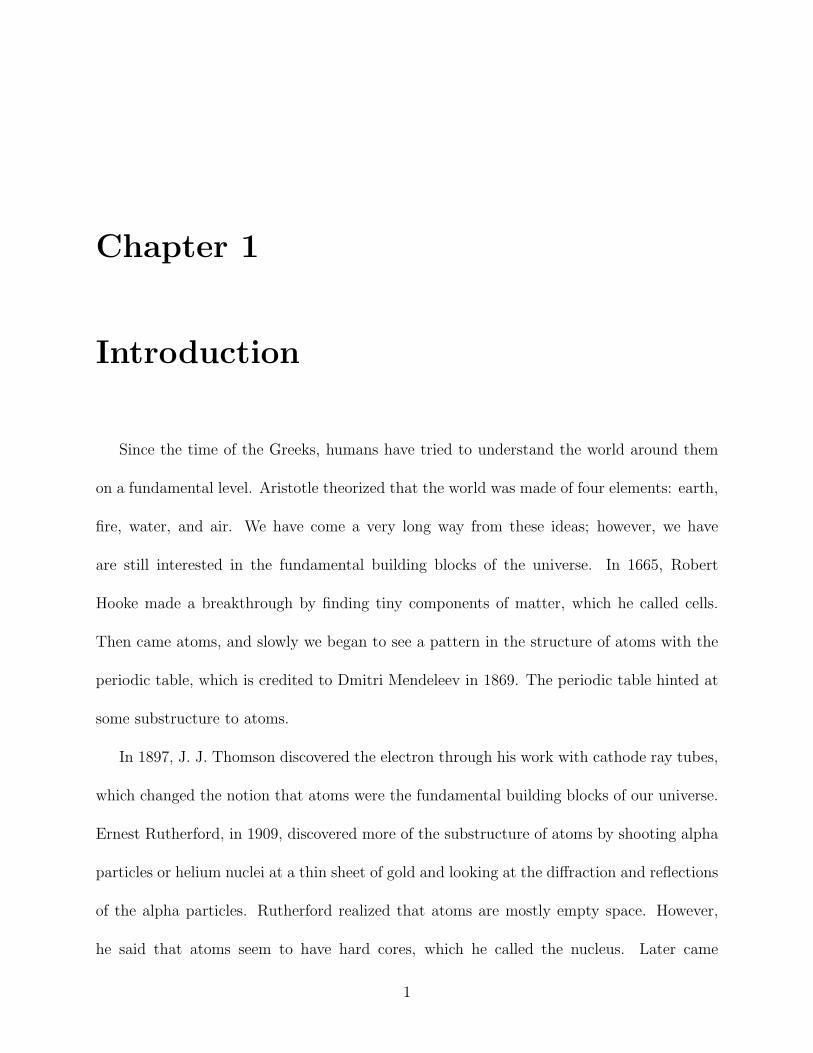
prediction of a new particle called the Ω−, which was later found in 1964. An example of the

structure that the eightfold way gave can be seen in Figure 1.1. It is interesting to look at

the eightfold way for its group theory background, and how mathematics has played a key

role in the progress of science from Einstein to Dirac.

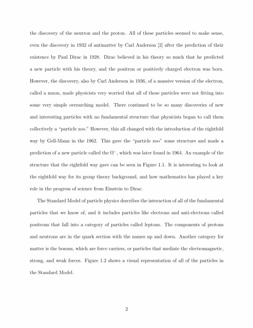
The Standard Model of particle physics describes the interaction of all of the fundamental

particles that we know of, and it includes particles like electrons and anti-electrons called

positrons that fall into a category of particles called leptons. The components of protons

and neutrons are in the quark section with the names up and down. Another category for

matter is the bosons, which are force carriers, or particles that mediate the electromagnetic,

strong, and weak forces. Figure 1.2 shows a visual representation of all of the particles in

the Standard Model.

2

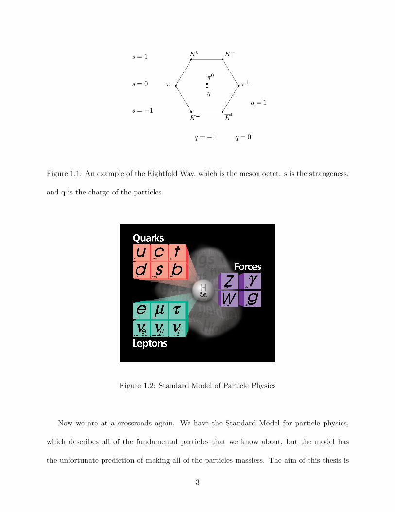
Figure 1.1: An example of the Eightfold Way, which is the meson octet. s is the strangeness,

and q is the charge of the particles.

Figure 1.2: Standard Model of Particle Physics

Now we are at a crossroads again. We have the Standard Model for particle physics,

which describes all of the fundamental particles that we know about, but the model has

the unfortunate prediction of making all of the particles massless. The aim of this thesis is

3

to improve the sensitivity to a particle called the Higgs boson, which will result from the

breaking of the electroweak symmetry of the Standard Model and give particles mass. This

is very important because we know that particles like the Z and W+/− bosons have a large

amount of mass. The Higgs boson is the simplest way of giving particles in the Standard

Model mass. There are other theories such as symmetry leaking to other dimensions [4],

technicolor [5], and top quark condensate [8], but they are beyond the scope of this paper.

The Large Electron-Positron (LEP) Collider, which was housed in the same ring as the

Large Hadron Collider (LHC) in Geneva, Switzerland, provides an experimental limit lower

bound on the Higgs boson mass of 114 GeV/c2. The LEP experiment also had approximately

a two standard deviation excess of Higgs events at a mass of 115.6 GeV/c2 [7], which is in

the mass range where my analysis is most sensitive. The TeVatron at Fermilab in Batavia,

Illinois has also ruled out the region around 160-170 GeV/c2 [3]. Finally, the theory work

that tells us that a higher mass Higgs is unlikely. This information is contained in Figure

1.3, which shows the mass regions that have been ruled out at 95% Confidence Level.

4

Figure 1.3: The Limits that have been placed on the Higgs bosons mass. The horizontal axis

is the mass of the Higgs boson, and the vertical axis represents the ∆χ2 probability of the

Higgs having a at the given mass. The yellow portions have been ruled out by experiment.

5

Chapter 2

Higgs Mechanism

The Higgs Mechanism is the easiest way to give mass to the particles in the Standard

Model, and it was discovered by Peter Higgs in 1964 as well as by Guralnik, Hagen, Kibble,

Brout, and Englert [6]. The Higgs Mechanism has the fortunate consequence of having a

particle called the Higgs Boson associated with it, which expermentalists can look for to

verify the Higgs field theory. It is interesting to note that Higgs’s paper in 1964 was rejected

by the Physics Review Letters journal because it made no measurable prediction, so Higgs

added a line at the end about creating one or more massive scalar particles [6]. Because of

that one line, the main push at the LHC is to find the “Higgs” boson.

The Higgs Mechanism is a spontaneous symmetry breaking model that allows for particles

to gain mass, and it requires a new field called the Higgs field which permeates all space

and has a non-zero vacuum expectation value. The Higgs field is a symmetric potential, like

the one in Figure 2.1. At some time in the past, the Higgs field slipped to a non-zero value,

which spontaneously broke the electroweak symmetry. The problem with any spontaneous

symmetry breaking model is that according to Goldstone’s Theorem there should be an

6

associated massless particle. However, we have not observed such a particle. Hence, the

Higgs Mechanism also needs to rule out such a Goldstone boson. Peter Higgs’s observation

was that combing a gauge theory with a spontaneously symmetry-breaking model causes the

massless boson to gain mass.

7

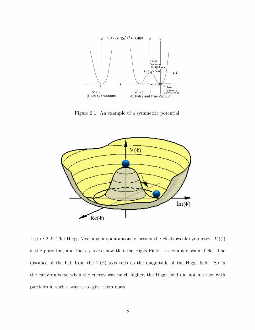
Figure 2.1: An example of a symmetric potential.

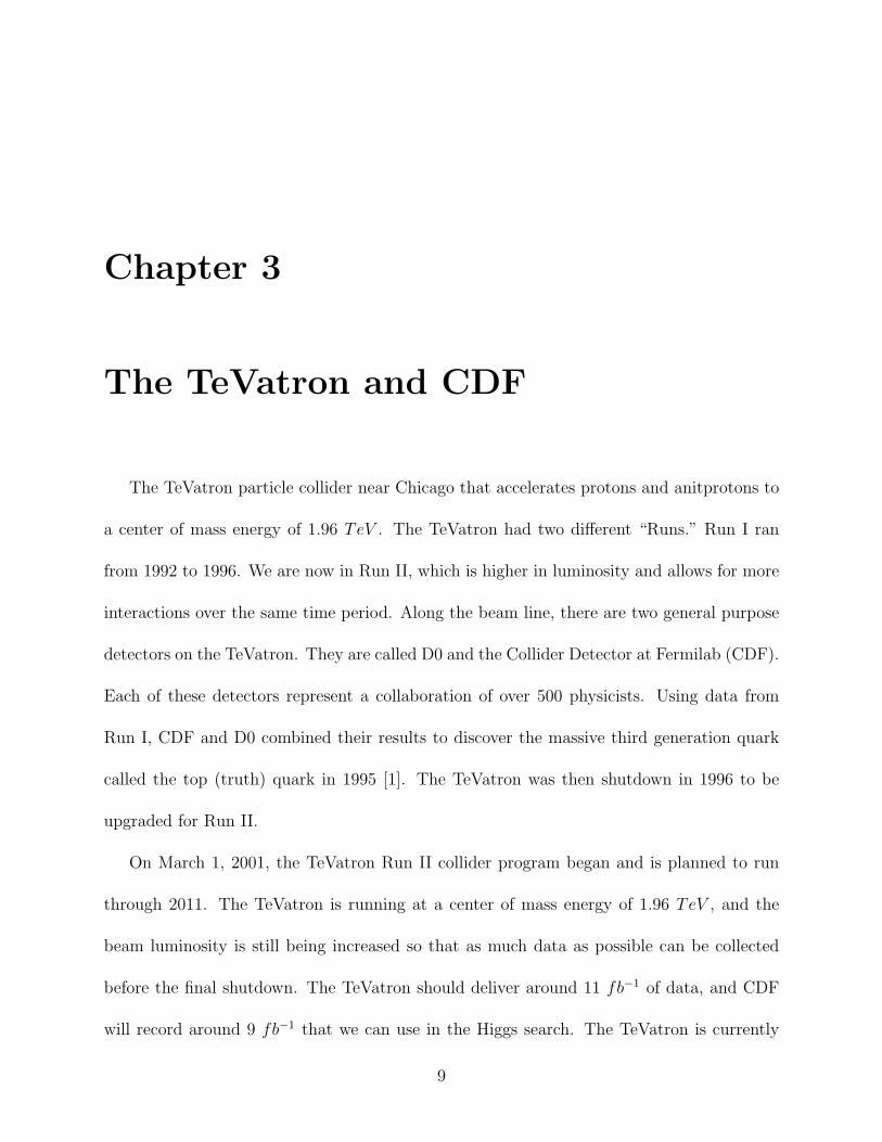
Figure 2.2: The Higgs Mechanism spontaneously breaks the electroweak symmetry. V (φ)

is the potential, and the x-y axes show that the Higgs Field is a complex scalar field. The

distance of the ball from the V (φ) axis tells us the magnitude of the Higgs field. So in

the early universe when the energy was much higher, the Higgs field did not interact with

particles in such a way as to give them mass.

8

Chapter 3

The TeVatron and CDF

The TeVatron particle collider near Chicago that accelerates protons and anitprotons to

a center of mass energy of 1.96 TeV . The TeVatron had two different “Runs.” Run I ran

from 1992 to 1996. We are now in Run II, which is higher in luminosity and allows for more

interactions over the same time period. Along the beam line, there are two general purpose

detectors on the TeVatron. They are called D0 and the Collider Detector at Fermilab (CDF).

Each of these detectors represent a collaboration of over 500 physicists. Using data from

Run I, CDF and D0 combined their results to discover the massive third generation quark

called the top (truth) quark in 1995 [1]. The TeVatron was then shutdown in 1996 to be

upgraded for Run II.

On March 1, 2001, the TeVatron Run II collider program began and is planned to run

through 2011. The TeVatron is running at a center of mass energy of 1.96 TeV , and the

beam luminosity is still being increased so that as much data as possible can be collected

before the final shutdown. The TeVatron should deliver around 11 fb−1 of data, and CDF

will record around 9 fb−1 that we can use in the Higgs search. The TeVatron is currently

9

the highest energy particle accelerator in the world. The TeVatron accelerates protons and

antiprotons around the 6.28 km circular tunnel. There are bunches of around 1014 protons

and antiprotons, which travel around main ring at a highly relativistic speed with bunch

crossings every 396 ns. A bunch crossing is the event when a proton cloud passes through

an antiproton cloud in the CDF or D0 detectors.

3.1 Collider Detector at Fermilab

The data I use is collected by CDF. The detector is capable of taking a large number of

measurements and identifying a wide variety of particles. We define a coordinate system in

the detector that I will use throughout the rest of this paper. The angles in the transverse

plane to the beam line are denoted by φ and vary between 0 and 2π. I will also discuss the

angle between objects when projected into the transverse plane to the beam line, and I will

denote these angles by ∆φ. Another angular measurement is the angle with respect to the

beam line, which is denoted by θ and varies between −π2

and +π2

. What is more important is

using θ to define the pseudorapidity, which is given by η = − ln[tan ( θ2)] and varies between

−∞ to ∞. Finally, we denote the total angular separation by ∆R =√

(∆φ)2 + (∆η)2.

I will now give an introduction to the different components of the detector. Starting at

the collision point and working outward, CDF has a wide variety of different components.

The protons and antiprotons are carried in the beam pipe. Immediately outside of the

beam pipe is silicon tracker, and it continues to 28 cm from the interaction point. The

newly created charged particles that leave transverse to the beam line from the interaction

point make a signature called a “hit” in some of the seven barrels of silicon. The barrels

10

are arranged in concentric circles, and the “hits” can be connected like dots to plot the

trajectory of the particles leaving the beam pipe. The silicon detector is placed in a strong

magnetic field which causes the charged particles like electron, muons, taus, and charged

hadrons to curve. This helps identify the electric charge of the particles by determining the

orientation of curvature. The silicon tracker is very sensitive and allows for the detection of

secondary interaction points. This is very important for the identification of b quarks because

they travel a small distance from the original interaction point before showering into other

particles. This is the hallmark sign of a b quark. As we will see later, the identification of b

quarks is important for the Higgs search.

The next layer of CDF is the Central Outer Tracker (COT) and goes from 28 cm to

1.3 m. The COT is filled with Argon and Ethane so that charged particles can ionize the

gas. The COT is also filled with tens of thousands of wires which are at high voltage to

collect the ions. The voltage causes the ions to cascade toward the wires and create more

electrons so that the signal is measurable. There are two types of wires called sense wires

and field wires. The sense wires detect the electrons which are ionized off of the atoms in

the gas. The field wires absorb the positive charges that are left behind from the electron

ionization.

The solenoid covers the COT and provides a strong magnetic field of 1.4 T to help identify

charged particles coming outward from the interaction point. The amount that the particles

bend also gives a measure of their momentum. The higher momentum particles have a lower

curvature while the lower momentum particles have a much higher curvature. The solenoid

is made of superconducting material and must be kept at 4.7 K to stay superconducting.

The B field from the solenoid effectively ends about 1.5 m from the beam line and is one of

11

the most important parts of the detector for the identification of charged particles.

Beyond the solenoid is the electromagnetic (EM) calorimeter, which measures the energy

of light particles like electrons and photons. The EM calorimeter is made of alternating

layers of plastic scintillator followed by 0.75 in thick sheets of lead. The change in materials

causes the high energy charged particles to emit Cerenkov radiation. Also the light electrons

emit light via Bremsstrahlung and slow down losing their energy in the scintillator. The

hadronic calorimeter surrounds the EM Calorimeter and measures the energy of particles

like protons and neutrons. The energy measurement of the neutron is the first signature

received from these neutral particles. The separation of neutral particles from charged ones

lies in the fact that charged particles should have a track that leads up to the calorimeter

tower.

The muon chambers are the most distant from the beam line, but are very important for

identifying the massive leptons. Since a lot of interesting particles like quarks can decay to

muons, it is important to identify them. The outer part of the muon chamber is essentially a

drift chamber with sense wires and is very similar to the COT, but these drift chambers are

very slow. Hence, some scintillating material was added because it can give a quick response

from the time of muon passing through the drift chamber. There is also a large amount of

steel to shield the outer layers of the muon chambers because we only want to detect muons.

Neutrinos can also pass through all of the steel; however, they are too weakly interacting to

be seen. So their existence is inferred from the conservation of momentum and energy and

not through any direct detection.

12

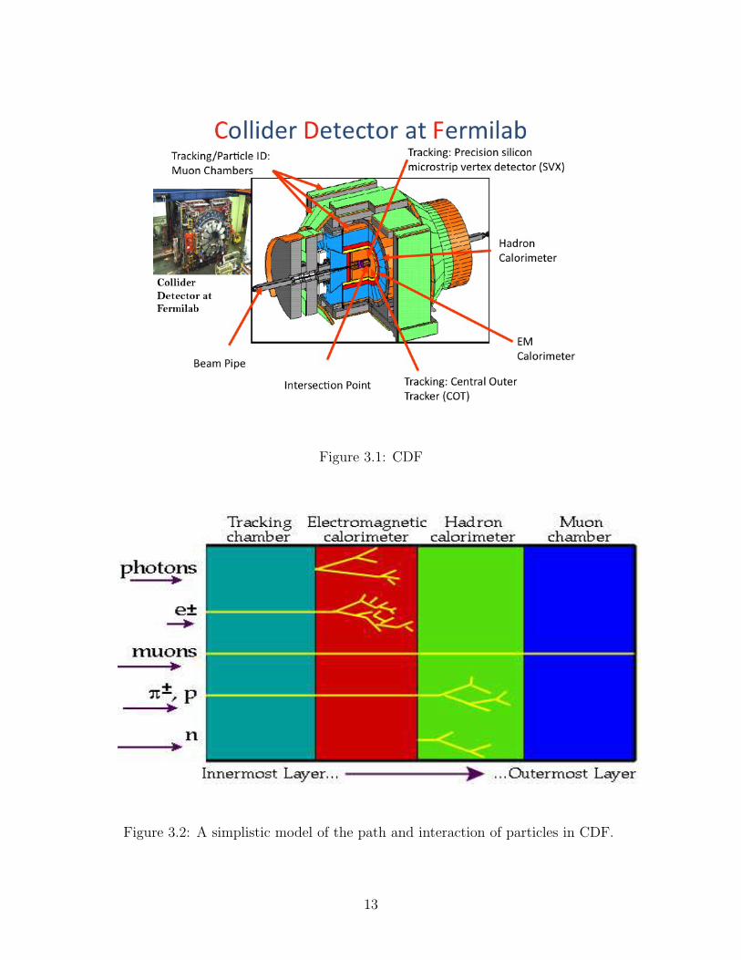
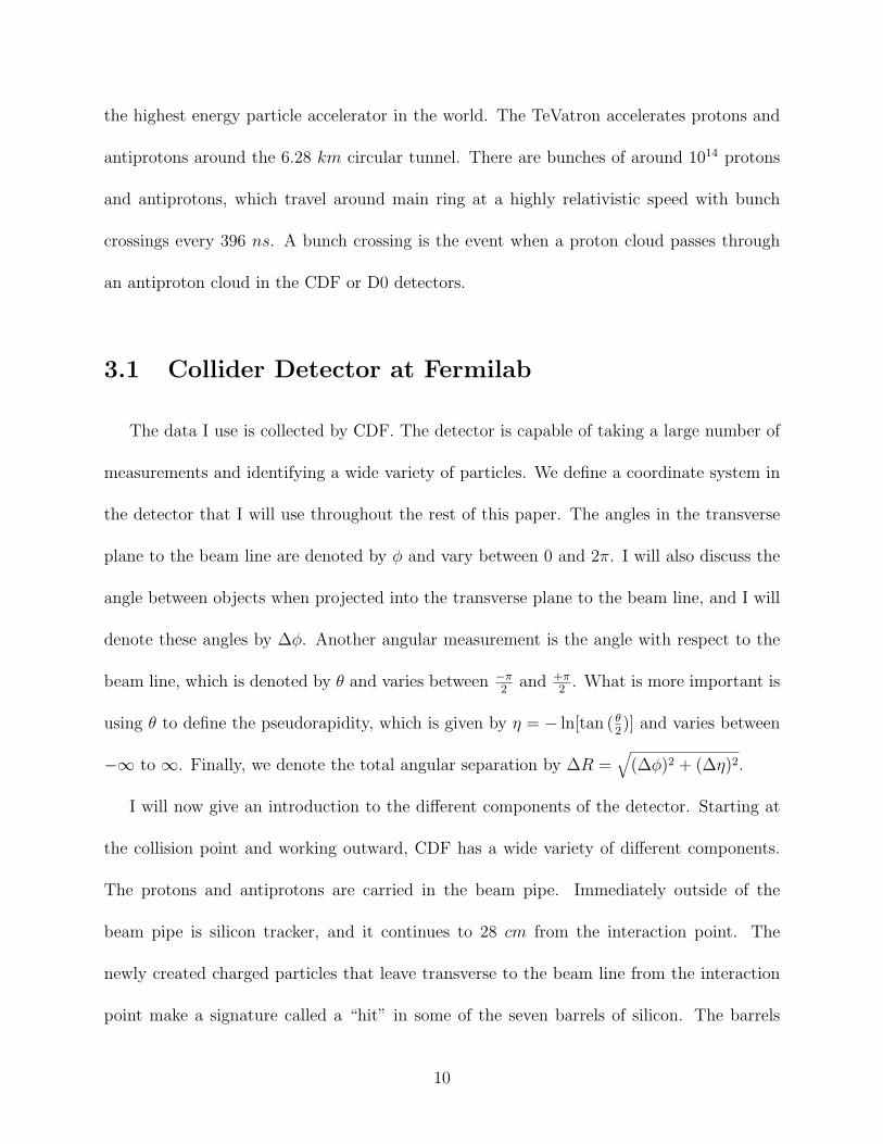
Figure 3.1: CDF

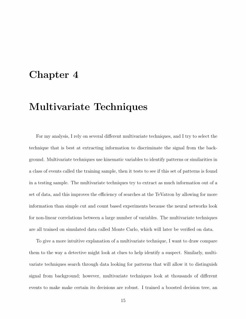
Figure 3.3: A simplistic portrayal of how particles behave within the CDF detector.

3.2.2 Silicon Tracking

Placed directly on the beam pipe, closest to the aftermath of a proton-antiproton

collision are the silicon detectors. The silicon detector is divided into three layered

sub-systems. Layer00 is the first sub-system, with the innermost layer positioned at

a radial distance of 1.35 cm around the beampipe. This layer must withstand the

greatest amount of radiation of any part of the detector, and is comprised of single

sided silicon wafers designed to tolerate the large bias voltages necessary. Layer 00

allows for enhanced resolution on the impact parameter associated with collisions,

and offers a layer of protection for the second silicon sub-system.

The SVX II is comprised of 5 layers of double-sided silicon. In each layer, one side

is axial, aligned to offer radial and transverse tracking information (r-φ), while the

36

Figure 3.2: A simplistic model of the path and interaction of particles in CDF.

13

3.2 Trigger System

The trigger system determines which of the 3 million collisions happening each second

should be recorded. The trigger has many different paths, but ultimately it is limited to

recording data at a rate no faster than 50 Hz. This is a factor of 50,000 smaller than the

frequency of bunch crossings. The trigger for CDF contains three levels with the first level

containing mostly hardware. The second level translates the hardware information into data

that can be read by software. The second level has around 20 µs to make its decision, so it

is pressed for time. The information is then read out for the third level of the trigger where

the event is completely reconstructed. For the purpose of this analysis, the trigger looks for

at least 2 clusters of more than 10 GeV in energy with at least one of them being central or

with |η| < 1. Also at least 35 GeV in missing transverse energy (MET) is required to keep

the event for this analysis.

14

Chapter 4

Multivariate Techniques

For my analysis, I rely on several different multivariate techniques, and I try to select the

technique that is best at extracting information to discriminate the signal from the back-

ground. Multivariate techniques use kinematic variables to identify patterns or similarities in

a class of events called the training sample, then it tests to see if this set of patterns is found

in a testing sample. The multivariate techniques try to extract as much information out of a

set of data, and this improves the efficiency of searches at the TeVatron by allowing for more

information than simple cut and count based experiments because the neural networks look

for non-linear correlations between a large number of variables. The multivariate techniques

are all trained on simulated data called Monte Carlo, which will later be verified on data.

To give a more intuitive explanation of a multivariate technique, I want to draw compare

them to the way a detective might look at clues to help identify a suspect. Similarly, multi-

variate techniques search through data looking for patterns that will allow it to distinguish

signal from background; however, multivariate techniques look at thousands of different

events to make make certain its decisions are robust. I trained a boosted decision tree, an

15

artificial neural network, and a support vector machine for ZH versus each background in-

dividually as well as WH versus each background individually.

4.1 Artificial Neural Networks

The are playing a fundamental role in the search for the Higgs boson. ANNs were used

in the 1.7 fb−1 analysis by giving them track information to separate backgrounds that were

in a large part due to poor detector resolution. Also an ANN was used as a discriminant for

the Higgs.

4.2 Boosted Decision Trees (BDT)

Boosted Decision Trees (BDT) are perhaps the simplest of the multivariate learning

techniques that I used; however, this did not stop it from being a strong performer. The

simplicity allows for the decision trees to effectively utilize more kinematic variables. The

BDTs also trains very quickly because it is entirely cut based. The BDT trains approximately

400 trees. Then the best combination of these 400 trees are used to create a single output

value called a discriminating value, which moves the signal events toward a value of 1 and

the background to a value of 0.

The BDT used is a binary decision process. Figure 4.1 shows the training for a decision

tree. The boosting refers to the training of more than one decision tree, and the weighted

combining of the trees with different signal and background normalizations reduces some

16

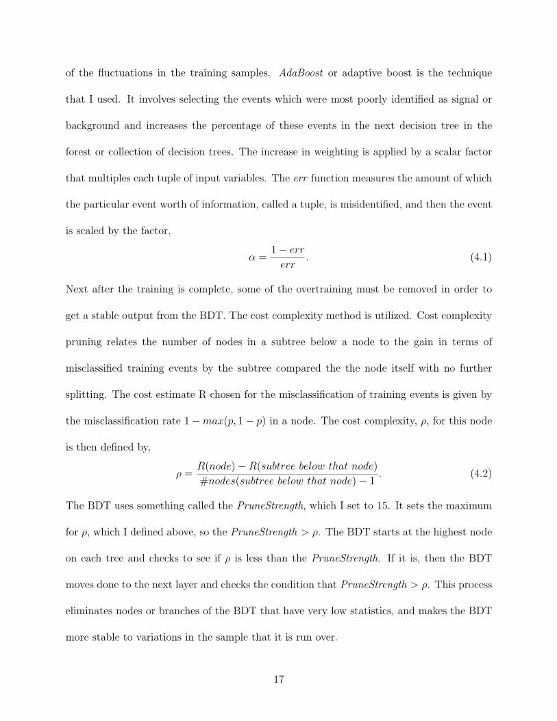
of the fluctuations in the training samples. AdaBoost or adaptive boost is the technique

that I used. It involves selecting the events which were most poorly identified as signal or

background and increases the percentage of these events in the next decision tree in the

forest or collection of decision trees. The increase in weighting is applied by a scalar factor

that multiples each tuple of input variables. The err function measures the amount of which

the particular event worth of information, called a tuple, is misidentified, and then the event

is scaled by the factor,

α =1− errerr

. (4.1)

Next after the training is complete, some of the overtraining must be removed in order to

get a stable output from the BDT. The cost complexity method is utilized. Cost complexity

pruning relates the number of nodes in a subtree below a node to the gain in terms of

misclassified training events by the subtree compared the the node itself with no further

splitting. The cost estimate R chosen for the misclassification of training events is given by

the misclassification rate 1−max(p, 1− p) in a node. The cost complexity, ρ, for this node

is then defined by,

ρ =R(node)−R(subtree below that node)

#nodes(subtree below that node)− 1. (4.2)

The BDT uses something called the PruneStrength, which I set to 15. It sets the maximum

for ρ, which I defined above, so the PruneStrength > ρ. The BDT starts at the highest node

on each tree and checks to see if ρ is less than the PruneStrength. If it is, then the BDT

moves done to the next layer and checks the condition that PruneStrength > ρ. This process

eliminates nodes or branches of the BDT that have very low statistics, and makes the BDT

more stable to variations in the sample that it is run over.

17

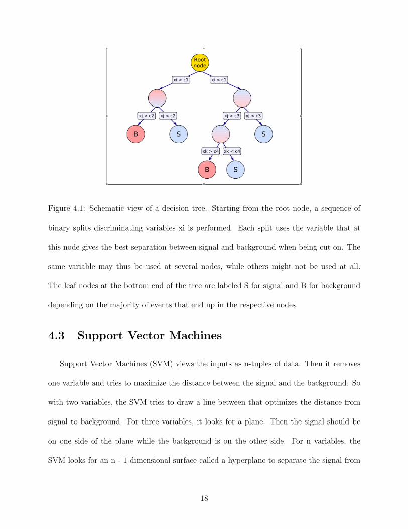
Figure 4.1: Schematic view of a decision tree. Starting from the root node, a sequence of

binary splits discriminating variables xi is performed. Each split uses the variable that at

this node gives the best separation between signal and background when being cut on. The

same variable may thus be used at several nodes, while others might not be used at all.

The leaf nodes at the bottom end of the tree are labeled S for signal and B for background

depending on the majority of events that end up in the respective nodes.

4.3 Support Vector Machines

Support Vector Machines (SVM) views the inputs as n-tuples of data. Then it removes

one variable and tries to maximize the distance between the signal and the background. So

with two variables, the SVM tries to draw a line between that optimizes the distance from

signal to background. For three variables, it looks for a plane. Then the signal should be

on one side of the plane while the background is on the other side. For n variables, the

SVM looks for an n - 1 dimensional surface called a hyperplane to separate the signal from

18

the background. The SVM takes a measurement of the distance from the hyperplane to the

event and uses this as its one dimensional output.

19

Chapter 5

ZH/WH → MET + Jets Analysis

5.1 Signals ZH and WH

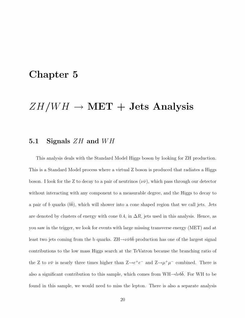
This analysis deals with the Standard Model Higgs boson by looking for ZH production.

This is a Standard Model process where a virtual Z boson is produced that radiates a Higgs

boson. I look for the Z to decay to a pair of neutrinos (νν), which pass through our detector

without interacting with any component to a measurable degree, and the Higgs to decay to

a pair of b quarks (bb), which will shower into a cone shaped region that we call jets. Jets

are denoted by clusters of energy with cone 0.4, in ∆R, jets used in this analysis. Hence, as

you saw in the trigger, we look for events with large missing transverse energy (MET) and at

least two jets coming from the b quarks. ZH→ννbb production has one of the largest signal

contributions to the low mass Higgs search at the TeVatron because the branching ratio of

the Z to νν is nearly three times higher than Z→e+e− and Z→µ+µ− combined. There is

also a significant contribution to this sample, which comes from WH→lνbb. For WH to be

found in this sample, we would need to miss the lepton. There is also a separate analysis

20

which aims to use the WH events; however, they require the identification of the lepton to

be included in their analyses. Therefore, WH provides an increase in the signal sample for

my analysis on ZH production, which is important because the production of the Higgs is so

small that we must try to collect as many events as possible.

Figure 5.1: Feynman Diagram for ZH Production

Figure 5.2: Feynman Diagram for WH Production

5.2 Backgrounds

5.2.1 QCD

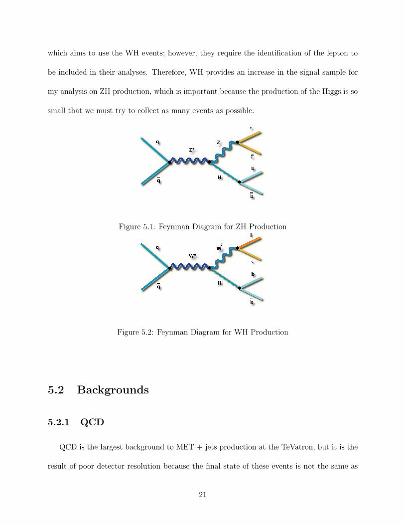
QCD is the largest background to MET + jets production at the TeVatron, but it is the

result of poor detector resolution because the final state of these events is not the same as

21

our signal. QCD events are produced at such a large rate that some are bound to enter the

sample.

Figure 5.3: One simple version of the QCD background.

5.2.2 Electroweak

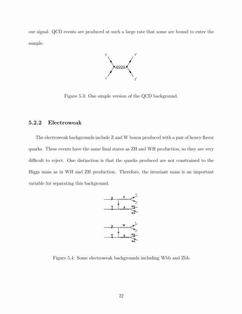
The electroweak backgrounds include Z and W boson produced with a pair of heavy flavor

quarks. These events have the same final states as ZH and WH production, so they are very

difficult to reject. One distinction is that the quarks produced are not constrained to the

Higgs mass as in WH and ZH production. Therefore, the invariant mass is an important

variable for separating this background.

Figure 5.4: Some electroweak backgrounds including Wbb and Zbb

22

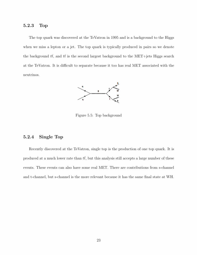
5.2.3 Top

The top quark was discovered at the TeVatron in 1995 and is a background to the Higgs

when we miss a lepton or a jet. The top quark is typically produced in pairs so we denote

the background tt, and tt is the second largest background to the MET+jets Higgs search

at the TeVatron. It is difficult to separate because it too has real MET associated with the

neutrinos.

Figure 5.5: Top background

5.2.4 Single Top

Recently discovered at the TeVatron, single top is the production of one top quark. It is

produced at a much lower rate than tt, but this analysis still accepts a large number of these

events. These events can also have some real MET. There are contributions from s-channel

and t-channel, but s-channel is the more relevant because it has the same final state at WH.

23

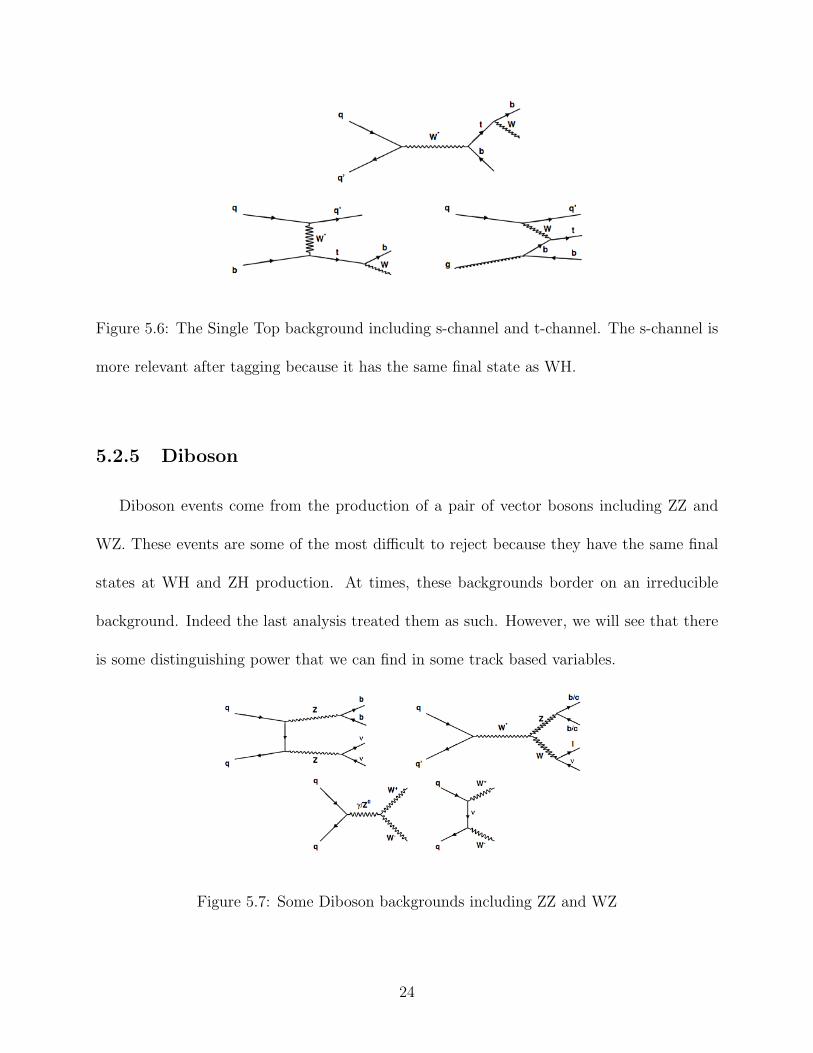
Figure 5.6: The Single Top background including s-channel and t-channel. The s-channel is

more relevant after tagging because it has the same final state as WH.

5.2.5 Diboson

Diboson events come from the production of a pair of vector bosons including ZZ and

WZ. These events are some of the most difficult to reject because they have the same final

states at WH and ZH production. At times, these backgrounds border on an irreducible

background. Indeed the last analysis treated them as such. However, we will see that there

is some distinguishing power that we can find in some track based variables.

Figure 5.7: Some Diboson backgrounds including ZZ and WZ

24

5.3 Selection Cuts

The various selection cuts for this analysis reduce the amount of background by a sig-

nificant amount. We hope that some cuts like the b tagging do not drastically change the

shape of the background and the signal because the training sets used in this analysis do not

require b tagging. But to take a limit of the Higgs cross-section we need to require b tagging

in order to cut the signal to background ratio to a more reasonable 1:50. While others cuts,

like the one on the angle φ between the two jets are used to define control regions for the

background. These regions are used to verify the Monte Carlo, which is simulated data used

to model the low cross-section Higgs events and their backgrounds. It is important to verify

that the Monte Carlo matches up with the data.

5.3.1 Kinematic Cuts

The MET also needs to be cleaned up to some extent, so we apply some requirements

on top of the MET35 Trigger. If more information is needed, then please consult Branon

Parks’ Thesis [9]. Here are the clean up cuts:

• At least one Z-Vertex with class > 11

• At least one track in the central tracking system with COT hits and PT > 0.5

• Require that at least 10% of the sum of all jet ET is deposited in the electromagnetic

calorimeter.

• Require that the total track PT over ET of all jets divided by the number of jets is

25

greater than 0.1.

1

Njet

Njet∑j=1

∑PT

ET> 0.1 (5.1)

• Jets that fall within 0.5 < η < 1.0 and 1.04 < η < 1.74 are often mismeasured. This

region, known as the chimney, contains a large amount of instrumentation and often

produces a second jet whose energy is measured low. Events with jets falling in this

region are vetoed.

• Tests of QCD modeling are performed in a region in which the MET is aligned with

the second jet. A large number of jets passing selection in this region are located at

|η| < 0.1. These events are removed in this region since the MET is likely due to the

instrumental effect of a large crack at η = 0. Studies of Pretag data (data prior to

tagging requirements) show that this effect is not present in the signal region.

Beyond eliminating fake MET , we also need to remove events that account for the turn on

of trigger efficiencies.

• Jets in the event are required to be separated by a cone of ∆R > 1.0 to avoid cluster

merging.

• A centrality requirement of |η| < 0.9 on at least one jet is applied due to the central

jet trigger requirement.

• A cut is placed on the missing transverse energy in the event. The MET in the event

must be recalculated after applying corrections to jets in the event. Only jets with

a raw ET > 10.0 GeV and |η| < 2.0 are corrected. The MET is then corrected by

the difference between raw and corrected ET for each jet. While the trigger threshold

26

for the uncorrected MET is set at 35 GeV , the efficiency is low for events with this

corrected MET . Therefore, a threshold of 50 GeV in corrected MET is set for an

event to be accepted.

The ZH→ννbb analysis makes some additional cuts in order to get a more pure sample

of the signal. The first set of cuts are to make sure that there are no electrons or muons in

the event coming from the primary vertex. Since a true Higgs event should have no high

energy electrons or muons coming from the interaction vertex in the final state, then we do

not want to find any in our detector. I will denote the following cuts by the name Tight

Cuts:

• Events with 2 and only 2 jets with ET > 20 GeV and |η| < 2.0(Tight) are accepted.

• If a third jet is found at high |η|(2.0 < |η| < 2.4) having a corrected ET > 20 GeV ,

the event is vetoed.

• In Higgs events, the leading jet is expected to be more energetic than that of most

backgrounds. A leading jet requirement of 45 GeV is placed on all events.

• Events with identied high-energy electrons and muons are not accepted, as these are

potential candidates for orthogonal WH searches. We implement the standard high-PT

definition of tight or loose leptons as a veto. However, we define a control region to

test trigger efficiencies and multivariate distributions as events with an identied high

PT muon.

• A cut is placed on events in which ∆φ(MET − LeadJet) < 0.8. This cut is highly

efficient for signal, and removes a portion of QCD background.

27

• The final cut placed on events is determined by the displacement between the MET

and the second jet. The region in which the MET is aligned with the second jet consists

almost entirely of multijet QCD production and is defined by ∆φ(MET−2ndJet) < 0.4.

A separate kinematic region dened by a cut of ∆φ(MET − 2ndJet) > 0.8 is used for

the final signal region and for studies of electroweak Monte Carlo backgrounds.

5.3.2 b Tagging

b tagging uses the fact that b quarks travel a distance from the interaction point, called

the primary vertex, to a secondary vertex before showering into a spray of particles called

a jet. The silicon tracking is very important for identifying the secondary vertex because

high Pt tracks can be traced back to look for intersections. Some of these intersections can

happen behind the primary vertex, and these events are called negative tags, which are used

to measure the systematic uncertainties of the b tagging. Tagging cuts out a large amount

of events without b quarks. The problem is that the efficiency for the for accepting Higgs

events after these cuts is low as can be seen in table 5.1.

28

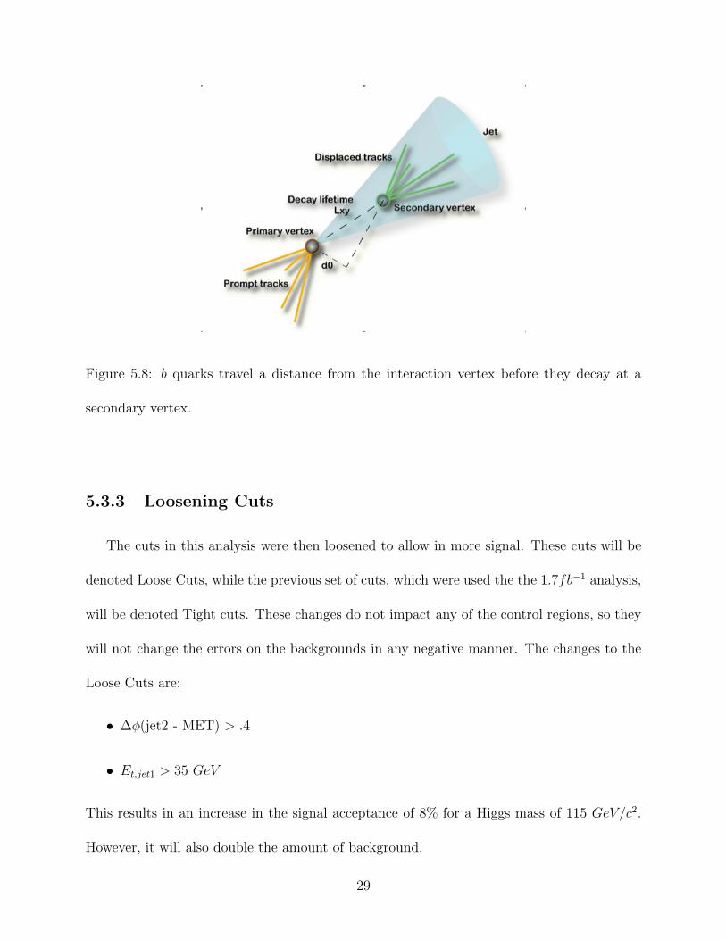
Figure 5.8: b quarks travel a distance from the interaction vertex before they decay at a

secondary vertex.

5.3.3 Loosening Cuts

The cuts in this analysis were then loosened to allow in more signal. These cuts will be

denoted Loose Cuts, while the previous set of cuts, which were used the the 1.7fb−1 analysis,

will be denoted Tight cuts. These changes do not impact any of the control regions, so they

will not change the errors on the backgrounds in any negative manner. The changes to the

Loose Cuts are:

• ∆φ(jet2 - MET) > .4

• Et,jet1 > 35 GeV

This results in an increase in the signal acceptance of 8% for a Higgs mass of 115 GeV/c2.

However, it will also double the amount of background.

29

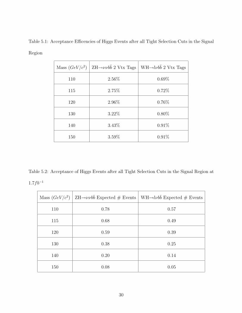
Table 5.1: Acceptance Efficencies of Higgs Events after all Tight Selection Cuts in the Signal

Region

Mass (GeV/c2) ZH→ννbb 2 Vtx Tags WH→lνbb 2 Vtx Tags

110 2.56% 0.69%

115 2.75% 0.72%

120 2.96% 0.76%

130 3.22% 0.80%

140 3.43% 0.91%

150 3.59% 0.91%

Table 5.2: Acceptance of Higgs Events after all Tight Selection Cuts in the Signal Region at

1.7fb−1

Mass (GeV/c2) ZH→ννbb Expected # Events WH→lνbb Expected # Events

110 0.78 0.57

115 0.68 0.49

120 0.59 0.39

130 0.38 0.25

140 0.20 0.14

150 0.08 0.05

30

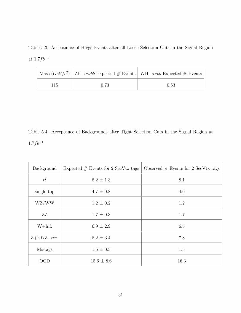
Table 5.3: Acceptance of Higgs Events after all Loose Selection Cuts in the Signal Region

at 1.7fb−1

Mass (GeV/c2) ZH→ννbb Expected # Events WH→lνbb Expected # Events

115 0.73 0.53

Table 5.4: Acceptance of Backgrounds after Tight Selection Cuts in the Signal Region at

1.7fb−1

Background Expected # Events for 2 SecVtx tags Observed # Events for 2 SecVtx tags

tt 8.2 ± 1.3 8.1

single top 4.7 ± 0.8 4.6

WZ/WW 1.2 ± 0.2 1.2

ZZ 1.7 ± 0.3 1.7

W+h.f. 6.9 ± 2.9 6.5

Z+h.f/Z→ττ . 8.2 ± 3.4 7.8

Mistags 1.5 ± 0.3 1.5

QCD 15.6 ± 8.6 16.3

31

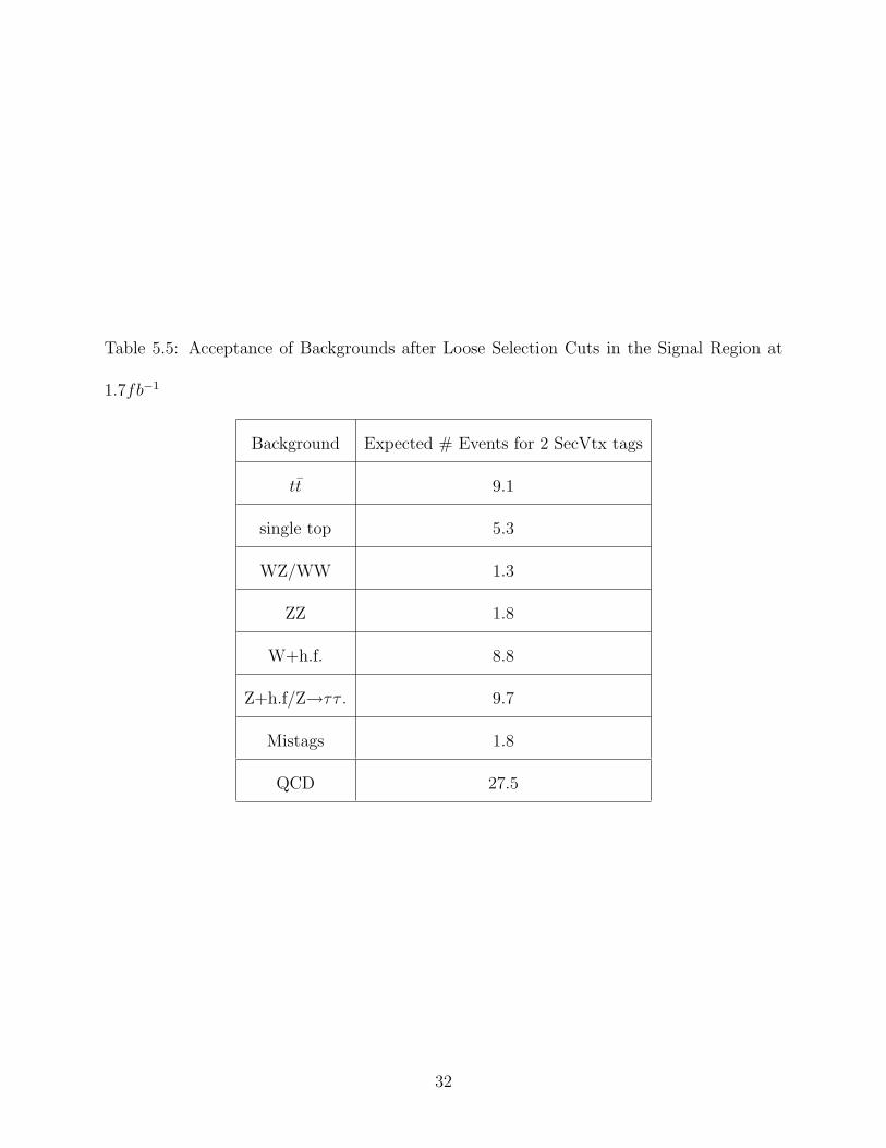
Table 5.5: Acceptance of Backgrounds after Loose Selection Cuts in the Signal Region at

1.7fb−1

Background Expected # Events for 2 SecVtx tags

tt 9.1

single top 5.3

WZ/WW 1.3

ZZ 1.8

W+h.f. 8.8

Z+h.f/Z→ττ . 9.7

Mistags 1.8

QCD 27.5

32

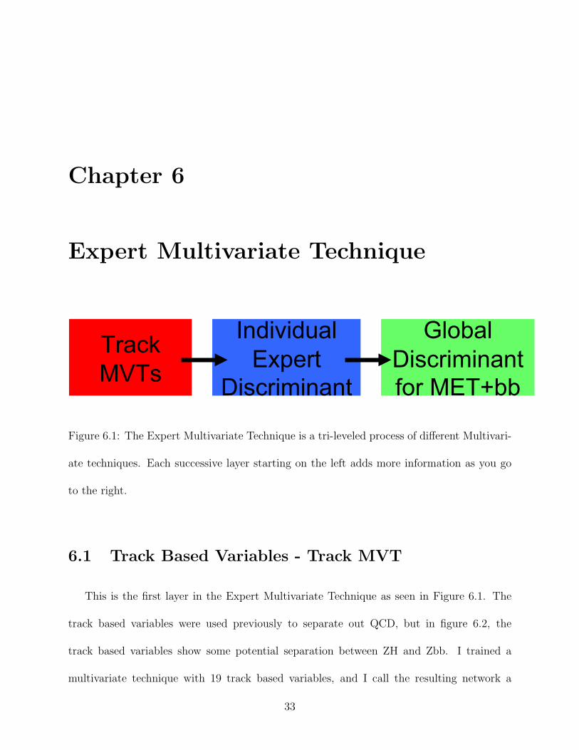
Chapter 6

Expert Multivariate Technique

Track MVTs

Global Discriminant for MET+bb

Individual Expert

Discriminant

Figure 6.1: The Expert Multivariate Technique is a tri-leveled process of different Multivari-

ate techniques. Each successive layer starting on the left adds more information as you go

to the right.

6.1 Track Based Variables - Track MVT

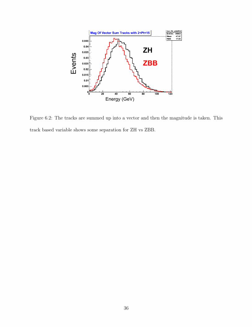
This is the first layer in the Expert Multivariate Technique as seen in Figure 6.1. The

track based variables were used previously to separate out QCD, but in figure 6.2, the

track based variables show some potential separation between ZH and Zbb. I trained a

multivariate technique with 19 track based variables, and I call the resulting network a

33

Track MVT, which looks for separation in ZH versus each of its backgrounds individually.

Then I also trained WH versus each of its backgrounds individually. The difference in

performance of these multivariate techniques justifies the separate training for WH and ZH.

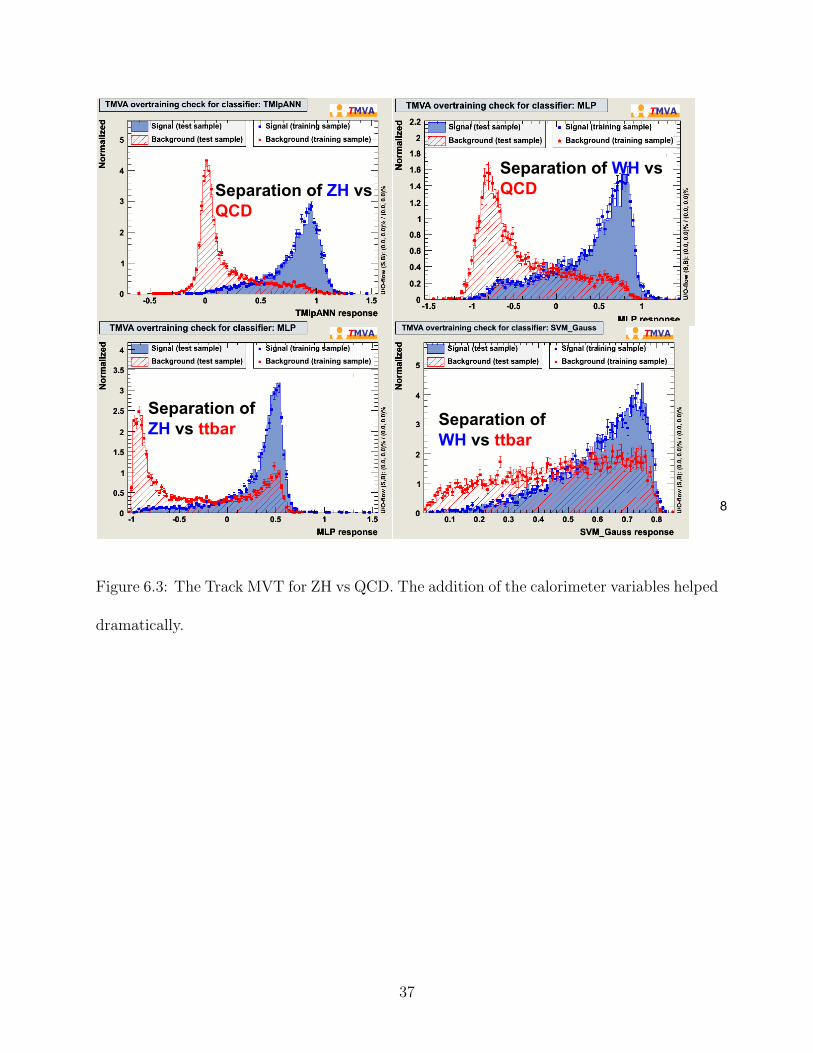
The better performance of the ZH networks can be seen in figure 6.3, in which ZH seems to

be better separated than WH from each background. The separation into one signal versus

one background at a time allows the multivariate technique to optimize for each background.

The best multivariate technique is chosen by collecting the largest integral under the curve

in the signal acceptance versus background rejection plot. In cases where the techniques are

very similar, then I refer to the KS test for the technique that seems to be modeled best.

An example of the signal versus background rejection plot can be seen in figure 6.4. The

definitions of the track based variables are listed below:

• metx0Q0Pt0 -∑

Px for all deftracks with PT > 0, χ2 < 2, and #COT hits > 0 1

• mety0Q0Pt0 -∑

Py for all deftracks with PT > 0, χ2 < 2, and #COT hits > 0 1

• etQ0Pt0 -∑

PT for all deftracks with PT > 0, χ2 < 2, and #COT hits > 0 1

• mezQ0Pt0 -∑

Pz for all deftracks with PT > 0, χ2 < 2, and #COT hits > 0 1

• metxQ6Pt2 -∑

Px for all deftracks with |ztrk position − zhigh PT trk| < 5cm, PT > 2,

χ2 < 2, and #COT hits > 0 1

• metyQ6Pt2 -∑

Py for all deftracks with |ztrk position − zhigh PT trk| < 5cm, PT > 2,

χ2 < 2, and #COT hits > 0 1

• etQ6Pt2 -∑

PT for all deftracks with |ztrk position − zhigh PT trk| < 5cm, PT > 2,

χ2 < 2, and #COT hits > 0 1

34

• metxQ1Pt2 -∑

Px for all deftracks with ≥ stereo/axialSL′s, 2 < PT > 15, χ2 < 2,

and #COT hits > 0 1

• metyQ1Pt2 -∑

Py for all deftracks with ≥ stereo/axialSL′s, 2 < PT > 15, χ2 < 2,

and #COT hits > 0 1

• etQ1Pt2 -∑

PT for all deftracks with ≥ stereo/axialSL′s, 2 < PT > 15, χ2 < 2,

and #COT hits > 0 1

• metxQ2Pt2 -∑

Px for all deftracks with 2 < PT > 15, χ2 < 2, and #COT hits > 0

1

• metyQ2Pt2 -∑

Py for all deftracks with 2 < PT > 15, χ2 < 2, and #COT hits > 0

1

• etQ2Pt2 -∑

PT for all deftracks with 2 < PT > 15, χ2 < 2, and #COT hits > 0 1

• maxPx - Find the max PT track with χ2 < 2 and #COThits > 0 and use its Px1

• maxPy - Find the max PT track with χ2 < 2 and #COThits > 0 and use its Py1

• nVtx - The number of class 12 vertices

• metQ0 - Which is defined by√

(metx0Q0Pt0)2 + (mety0Q0Pt0)2

• metSigQ0 - Which is defined by etQ0Pt0√(metx0Q0Pt0)2+(mety0Q0Pt0)2

• metQ6 - Which is defined by√

(metxQ6Pt0)2 + (metyQ6Pt0)2

1

1χ2 = χ2CT(# COT hits−5) < 2

35

ZH

ZBB E

vent

s

Energy (GeV)

Figure 6.2: The tracks are summed up into a vector and then the magnitude is taken. This

track based variable shows some separation for ZH vs ZBB.

36

8

Separation of WH vs QCD Separation of ZH vs

QCD

Separation of ZH vs ttbar Separation of

WH vs ttbar

Figure 6.3: The Track MVT for ZH vs QCD. The addition of the calorimeter variables helped

dramatically.

37

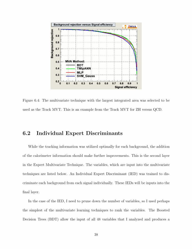
Figure 6.4: The multivariate technique with the largest integrated area was selected to be

used as the Track MVT. This is an example from the Track MVT for ZH versus QCD.

6.2 Individual Expert Discriminants

While the tracking information was utilized optimally for each background, the addition

of the calorimeter information should make further improvements. This is the second layer

in the Expert Multivariate Technique. The variables, which are input into the multivariate

techniques are listed below. An Individual Expert Discriminant (IED) was trained to dis-

criminate each background from each signal individually. These IEDs will be inputs into the

final layer.

In the case of the IED, I need to prune down the number of variables, so I used perhaps

the simplest of the multivariate learning techniques to rank the variables. The Boosted

Decision Trees (BDT) allow the input of all 48 variables that I analyzed and produces a

38

rank-ordered list of these variables. All variables of at least 1% significance according to

the BDT variable ranking were selected, and this lead to an average of 19 variables in each

Individual Expert Discriminant. As for the type of multivariate technique, the BDT, SVM

- Gauss, and ANN were all trained, and then the top performing multivariate technique was

chosen by the same method as the Track MVT. The complete list of variables is listed below:

1. L5 vertex corrected MET, which I have denoted MET and is defined by

MET = METcorr = METraw −#jets∑j=1

(EL5 corrT,j − EL5 raw

T,j ) (6.1)

2. ∆R(jet1, jet2)

3. Invariant mass of the lead jet and trailing jet -

M =

√√√√(2∑j=1

Ej)2 − (

2∑j=1

Px,j)2 − (

2∑j=1

Py,j)2 − (

2∑j=1

Pz,j)2 (6.2)

4. Track based neural network trained to separate ZH from QCD and was used in the

previous analysis

5. Track MET vector dotted with the L5 vertex corrected MET vector

6.#loose jets∑

j=1

ET,j, with loose jets being defined as having PT > 12 GeV and not the lead

or trailing jet

7. ∆φ(TrackMET,L5correctedMET )

8. Fox Wolfram 1 [9]

9. Fox Wolfram 2 [9]

39

10.

MT,norm =

√√√√(2∑j=1

Ej)2 − (

2∑j=1

Px,j)2 − (

2∑j=1

Py,j)2

ET,lead jet + ET,2ndjet

(6.3)

11. ET,lead jet

12. ET,2ndjet

13. ET,lead jet + ET,2ndjet

14. ET,lead jet + ET,2ndjet +#loose jets∑

j=1

ET,j

15. ∆φ(lead jet,MET )

16. ∆φ(2ndjet,MET )

17. ∆φ(lead jet, 2ndjet)

18. Track MVT for ZH versus QCD

19. Track MVT for ZH versus Diboson

20. Track MVT for ZH versus tt

21. Track MVT for ZH versus Single top

22. Track MVT for ZH versus WBB

23. Track MVT for ZH versus ZBB

24. Track MVT for WH versus QCD

25. Track MVT for WH versus Diboson

40

26. Track MVT for WH versus tt

27. Track MVT for WH versus Single top

28. Track MVT for WH versus WBB

29. Track MVT for WH versus ZBB

30. All 19 of the track variables listed above in section 6.1

WH vs. Ttbar ZH vs. Ttbar

WH vs. QCD

ZH vs. QCD

Figure 6.5: The individual expert discriminant for ZH vs QCD. The addition of the calorime-

ter variables helped dramatically.

41

6.3 Global Discriminant

Combining the Individual Expert Discriminant and 5 important kinematic variables re-

sults in the Global Expert Discriminant. This is a Jetnet based neural network, which was

the choice I made because the last neural network was also a Jetnet ANN. This made it easy

to do some direct comparisons. The additional 5 kinematic variables are the variables that

were used in the past analysis, except I switched the track ANN for ZH versus QCD for the

loose jet energy. Here is a list of the inputs:

1. MET as defined in equation 6.1

2. ∆R(jet1, jet2)

3. Invariant Mass as defined in equation 6.2

4. Track MET • L5 vertex corrected MET

5.#loose jets∑

j=1

ET,j as defined in Section 6.2

6. All of the Individual Expert Discriminants found in Section 6.2

42

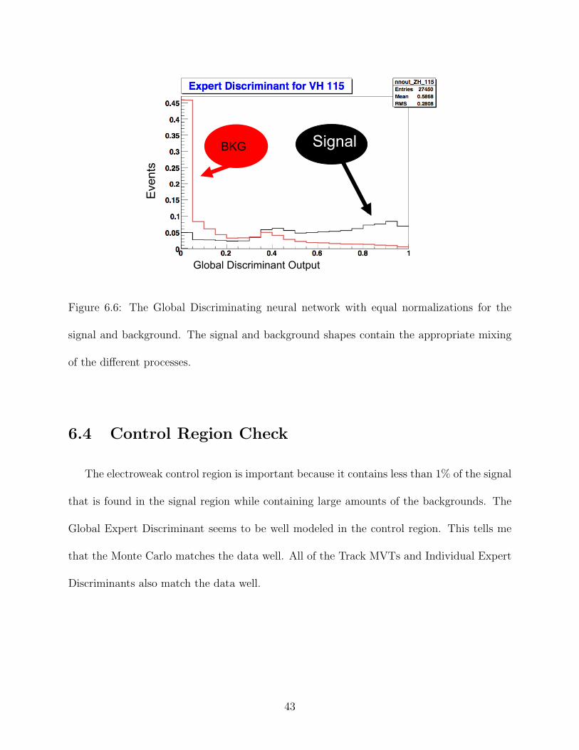
Eve

nts

Signal BKG

Global Discriminant Output

Figure 6.6: The Global Discriminating neural network with equal normalizations for the

signal and background. The signal and background shapes contain the appropriate mixing

of the different processes.

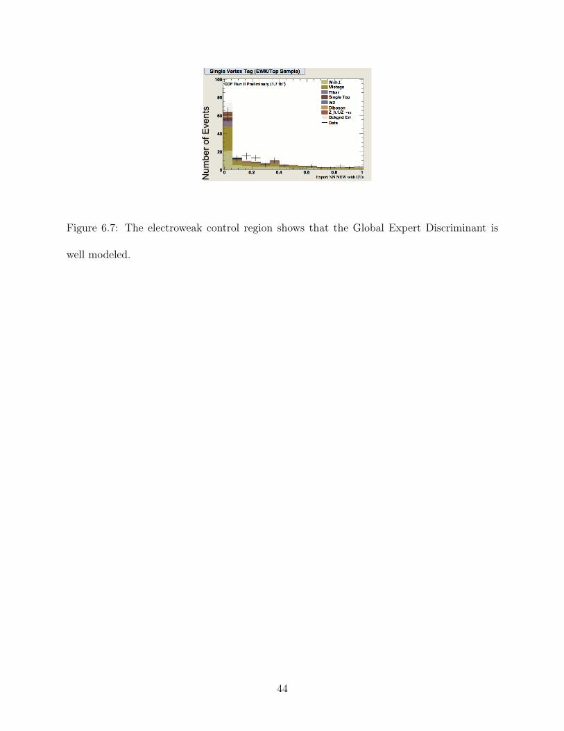
6.4 Control Region Check

The electroweak control region is important because it contains less than 1% of the signal

that is found in the signal region while containing large amounts of the backgrounds. The

Global Expert Discriminant seems to be well modeled in the control region. This tells me

that the Monte Carlo matches the data well. All of the Track MVTs and Individual Expert

Discriminants also match the data well.

43

Num

ber o

f Eve

nts

Figure 6.7: The electroweak control region shows that the Global Expert Discriminant is

well modeled.

44

Chapter 7

95% Expected Confidence Level

Limits on the Standard Model Higgs

Production

In order for us to just perform a counting experiment on the expectation of 50 background

events. To compare with the current expected statistical limits placed on Higgs boson at

115 GeV/c2, I want to ask how much data would we need to collect to obtain the same

upper limit on the Higgs production rate. The upper statistical limit on the expected Higgs

cross-section at 95% confidence is 9.2 times the expected Standard Model cross-section. So I

will calculate the number of trials or collections of 1.7 fb−1 that will be necessary to place the

same limit. If the upper limit is 9.2∗SM , then we would expect to see 9.2 Higgs events with

1.7 fb−1 of data. The null hypothesis is 48 background events. So we ask how much data

is needed to see a difference in a mean of 58.8 events and 48 events at 95% confidence. We

45

calculate two quantities for this test: the error given by N1/2 and the mean of 58.8 events.

Then to get to a 95% confidence upper bound on the Higgs production we would need to

collect 2.8 times as much data to place the same limits with a counting experiment as what

we do with the artificial neural network used in the 1.7 fb−1 analysis. So we do better than

a simple counting experiment.

7.1 Double SecVtx Tagged Events

The two tight SecVtx tagging category is one of two signal tagging regions. I ran the limit

calculations on these events to gauge the performance of the discriminant described in chapter

7. I expect the other tagging category with one tight SecVtx tag and one loose Jet Prob tag

will see comparable improvement. The limits were run with shapes coming from untagged

events because the statistics were much higher, and the shapes do not change sufficiently after

requiring tagging. The normalizations for the signal and background events came from the

two tight SecVtx tag numbers. Each limit was run on an independent sample to eliminate any

overtraining. In order to measure the improvement of the Global Discriminant, I compare

the results from the 1.7fb−1 neural network with the new global discriminant. Once the

cuts are loosened, the 95% Confidence Level Expected Limit for the 1.7fb−1 neural network

remains unchanged. In a direct comparison, the Global Expert Discriminant improves the

a priori limit by 14%, which can be seen in table 7.1. The 95% Confidence Level Expected

Limits are reported as the limit multiplied by the Standard Model expected cross-section,

and we want to see this limit approach one before we can say anything about the Higgs

production. The limit is analogous to asking how large would the Higgs cross-section have

46

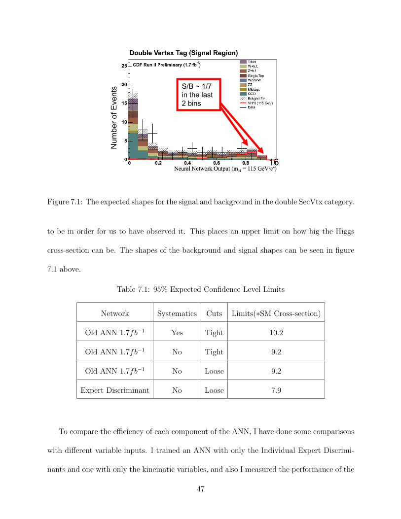
Num

ber o

f Eve

nts

16

S/B ~ 1/7 in the last 2 bins

Figure 7.1: The expected shapes for the signal and background in the double SecVtx category.

to be in order for us to have observed it. This places an upper limit on how big the Higgs

cross-section can be. The shapes of the background and signal shapes can be seen in figure

7.1 above.

Table 7.1: 95% Expected Confidence Level Limits

Network Systematics Cuts Limits(∗SM Cross-section)

Old ANN 1.7fb−1 Yes Tight 10.2

Old ANN 1.7fb−1 No Tight 9.2

Old ANN 1.7fb−1 No Loose 9.2

Expert Discriminant No Loose 7.9

To compare the efficiency of each component of the ANN, I have done some comparisons

with different variable inputs. I trained an ANN with only the Individual Expert Discrimi-

nants and one with only the kinematic variables, and also I measured the performance of the

47

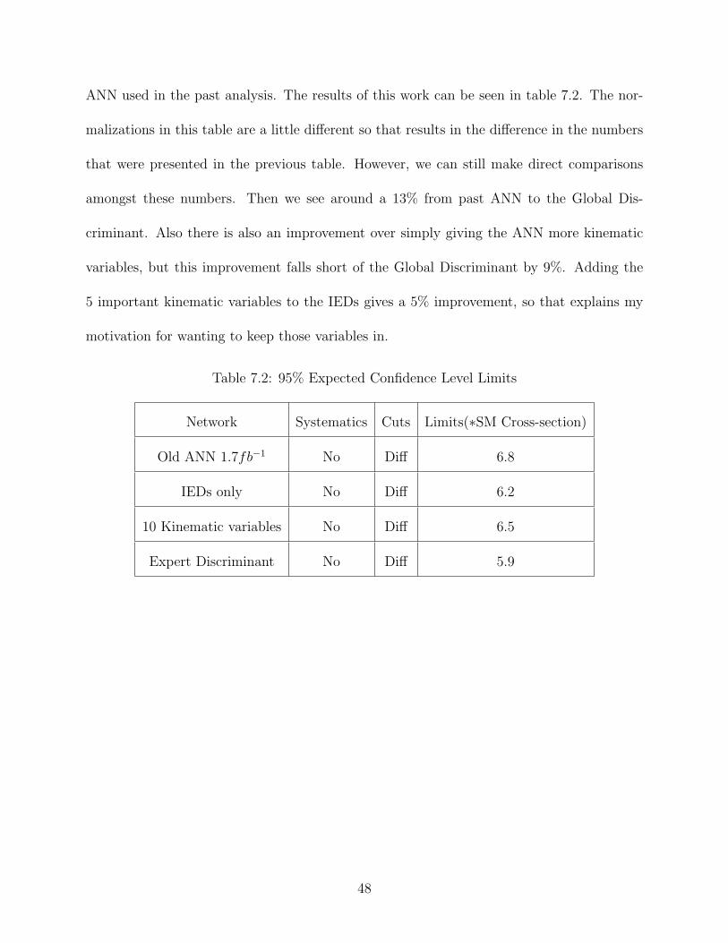
ANN used in the past analysis. The results of this work can be seen in table 7.2. The nor-

malizations in this table are a little different so that results in the difference in the numbers

that were presented in the previous table. However, we can still make direct comparisons

amongst these numbers. Then we see around a 13% from past ANN to the Global Dis-

criminant. Also there is also an improvement over simply giving the ANN more kinematic

variables, but this improvement falls short of the Global Discriminant by 9%. Adding the

5 important kinematic variables to the IEDs gives a 5% improvement, so that explains my

motivation for wanting to keep those variables in.

Table 7.2: 95% Expected Confidence Level Limits

Network Systematics Cuts Limits(∗SM Cross-section)

Old ANN 1.7fb−1 No Diff 6.8

IEDs only No Diff 6.2

10 Kinematic variables No Diff 6.5

Expert Discriminant No Diff 5.9

48

Chapter 8

Conclusions

The Expert Multivariate Technique results in a 14% improvement in the 95% confidence

level a priori expected statistical limit for the Higgs Boson in the ZH→ννbb analysis. The

quoted improvements are based on the improvement in events with two tight b tags. The

training for the all of the discriminants do not require any form of tagging for the events.

However, upon comparison of the shapes of the different backgrounds, the b tagging require-

ment causes no significant change in the shape of the backgrounds or signals. Hence, I expect

to see similar improvement with the other tagging selections. If this is the case, then then

one way to view the improvements is to say that we would have had to collect 30% more

data to see the same improvements with the old analysis technique.

As far as the systematic errors, I expect them to scale with the statistical improvements

as has been seen in past analyses. In the future, the increase in data will allow us to put

tighter constraints on the backgrounds, which decreases our systematic errors; therefore, the

systematic errors can change with the amount of data and in general decrease along with

statistical errors.

49

Some important features of the Expert Multivariate Technique is that it optimizes the

separation of each signal from each background individually. The Individual Expert Dis-

criminants allows for the selection of the most important distinguishing variables for each

background before training a Global Expert Discriminant. These separate trainings allow

the multivariate techniques to better account for the differences in the WH and ZH signals,

which was motivated by the differing performance of the ZH networks versus the WH net-

works. Since the Expert Multivariate Technique (EMT) optimizes the separation of each

background as well as incorporating the tracking information as another discriminant, it

reduces the total amount of background in the signal like region, which allows us to open

the cuts and accept more signal. The EMT deals with the extra background in a far more

effective way than the old 1.7 fb−1 neural network does.

Finally, the EMT is very general and does not require anything that is unique to the

ZH→ννbb channel; therefore, I believe that these ideas could fairly easily be extended to

other analysis like ZH→e+e−bb and WH→lνbb. I would expect to see similar increases

in sensitivity to the Higgs in these other channels. For example, the separation from the

tracking information could be used to improve the dijet mass resolution in the ZH→e+e−bb

analysis by getting a better gauge on some of the fake MET in the event. In this channel,

the information from the pair of electrons is used to apply a correction to the b jets, and the

correction improves the resolution of the dijet mass as well as the momentum and energy

of the jets. Other ideas for improvement are to investigate the use of a boosted decision

tree as the final discriminant instead of the Jetnet neural network. Also a check to see how

much improvement we get from just giving a boosted decision tree all of the variables is

important to show that the Individual Expert Discriminants are needed. Finally, I plan to

50

add in systematics as well as the other tagging categories. Most of these tests are in progress

and should be completed this summer.

The EMT improves our sensitivity to the Higgs boson, which is the simplest way of giving

particles in the Standard Model mass. It is important to find the Higgs because it can tell us

a lot about new physics. Also there is always the chance that the Higgs does not exist, which

poses an even more exciting proposition because it means that we really do not understand

the universe. Only time will tell whether the Higgs exists, but until then the Large Hadron

Collider will be starting up and will give us the opportunity to study the universe at a much

higher energy and on a grander scale.

51

Bibliography

[1] F. Abe, H. Akimoto, A. Akopian, M. G. Albrow, S. R. Amendolia, D. Amidei, J. An-

tos, C. Anway-Wiese, S. Aota, G. Apollinari, T. Asakawa, W. Ashmanskas, M. Atac,

P. Auchincloss, F. Azfar, P. Azzi-Bacchetta, N. Bacchetta, W. Badgett, S. Bagdasarov,

M. W. Bailey, J. Bao, P. de Barbaro, A. Barbaro-Galtieri, V. E. Barnes, B. A. Barnett,

P. Bartalini, and G. Bauer. Observation of top quark production in pp collisions with

the collider detector at fermilab. Phys. Rev. Lett., 74(14):2626–2631, Apr 1995.

[2] Carl D. Anderson. The positive electron. Phys. Rev., 43(6):491–494, Mar 1933.

[3] CDF and D0 Collaborations. Combined cdf and d0 upper limits on standard model higgs-

boson production with up to 4.2fb−1 of data. FERMILAB-PUB-09-060-E, CDF(Note

9713):1–25, 2009.

[4] Csaba Csaki, Christophe Grojean, Luigi Pilo, and John Terning. Towards a realistic

model of higgsless electroweak symmetry breaking. Phys. Rev. Lett., 92(10):101802, Mar

2004.

[5] Savas Dimopoulos and Leonard Susskind. Mass without scalars. Nuclear Physics B,

155(1):237 – 252, 1979.

52

[6] Peter W. Higgs. Broken symmetries and the masses of gauge bosons. Phys. Rev. Lett.,

13(16):508–509, Oct 1964.

[7] Marumi M. Kado and Christopher G. Tully. The searches for higgs bosons at lep. Annual

Review of Nuclear and Particle Science, 52(1):65–113, 2002.

[8] Vladimir A. Miransky, Masaharu Tanabashi, and Koichi Yamawaki. Dynamical elec-

troweak symmetry breaking with large anomalous dimension and t quark condensate.

Nuclear Physics B, 221(1):177, 1989.

[9] Brandon Parks. Search for the higgs boson in the zh → ννbb channel at cdf run ii.

Technical report, Ohio State Physics Department, 2008.

53