Funky Mechanics Concepts - University of California, San Diego · 2018-10-30 · The Funky Series...
88
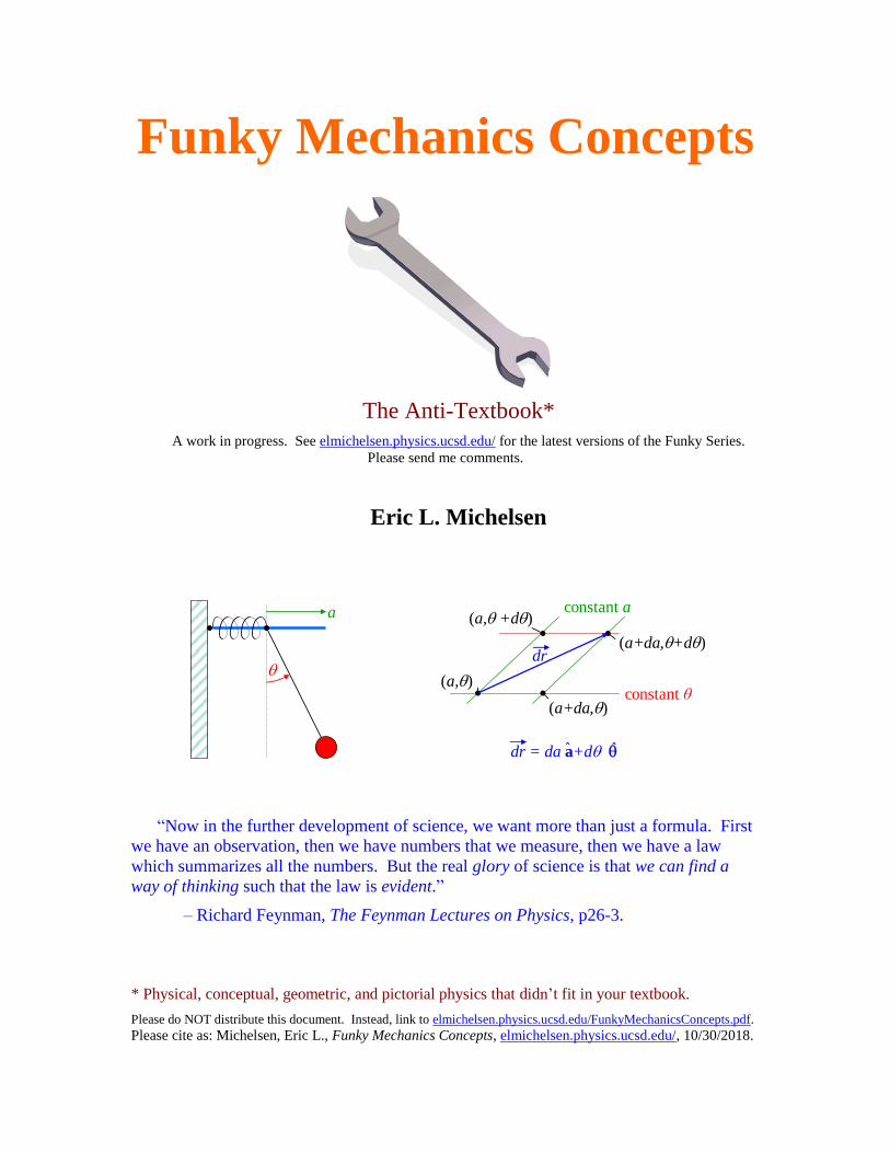
Funky Mechanics Concepts The Anti-Textbook* A work in progress. See elmichelsen.physics.ucsd.edu/ for the latest versions of the Funky Series. Please send me comments. Eric L. Michelsen a (a,) (a+da,) (a, +d) (a+da,+d) constant θ constant a dr = da a+d ˆ ˆ dr “Now in the further development of science, we want more than just a formula. First we have an observation, then we have numbers that we measure, then we have a law which summarizes all the numbers. But the real glory of science is that we can find a way of thinking such that the law is evident.” – Richard Feynman, The Feynman Lectures on Physics, p26-3. * Physical, conceptual, geometric, and pictorial physics that didn’t fit in your textbook. Please do NOT distribute this document. Instead, link to elmichelsen.physics.ucsd.edu/FunkyMechanicsConcepts.pdf. Please cite as: Michelsen, Eric L., Funky Mechanics Concepts, elmichelsen.physics.ucsd.edu/, 10/30/2018.
Transcript of Funky Mechanics Concepts - University of California, San Diego · 2018-10-30 · The Funky Series...
Funky Mechanics Concepts
The Anti-Textbook*
A work in progress. See elmichelsen.physics.ucsd.edu/ for the latest versions of the Funky Series.
Please send me comments.
Eric L. Michelsen
a
(a,)
(a+da,)
(a, +d)
(a+da,+d)
constant θ
constant a
dr = da a+d ˆ ˆ
dr
“Now in the further development of science, we want more than just a formula. First
we have an observation, then we have numbers that we measure, then we have a law
which summarizes all the numbers. But the real glory of science is that we can find a
way of thinking such that the law is evident.”
– Richard Feynman, The Feynman Lectures on Physics, p26-3.
* Physical, conceptual, geometric, and pictorial physics that didn’t fit in your textbook.
Please do NOT distribute this document. Instead, link to elmichelsen.physics.ucsd.edu/FunkyMechanicsConcepts.pdf.
Please cite as: Michelsen, Eric L., Funky Mechanics Concepts, elmichelsen.physics.ucsd.edu/, 10/30/2018.
elmichelsen.physics.ucsd.edu/ Funky Mechanics Concepts emichels at physics.ucsd.edu
10/30/2018 13:29 Copyright 2002 - 2018 Eric L. Michelsen. All rights reserved. 2 of 88
2006 values from NIST. For more physical constants, see http://physics.nist.gov/cuu/Constants/ .
Speed of light in vacuum c = 299 792 458 m s–1 (exact)
Gravitational constant G = 6.674 28(67) x 10–11 m3 kg–1 s–2
Relative standard uncertainty ±1.0 x 10⁻⁴
Boltzmann constant k = 1.380 6504(24) x 10–23 J K–1
Stefan-Boltzmann constant σ = 5.670 400(40) x 10–8 W m–2 K–4
Relative standard uncertainty ±7.0 x 10⁻⁶
Avogadro constant NA, L = 6.022 141 79(30) x 1023 mol–1
Relative standard uncertainty ±5.0 x 10⁻⁸
Molar gas constant R = 8.314 472(15) J mol-1 K-1
calorie 4.184 J (exact)
Electron mass me = 9.109 382 15(45) x 10–31 kg
Proton mass mp = 1.672 621 637(83) x 10–27 kg
Proton/electron mass ratio mp/me = 1836.152 672 47(80)
Elementary charge e = 1.602 176 487(40) x 10–19 C
Electron g-factor ge = –2.002 319 304 3622(15)
Proton g-factor gp = 5.585 694 713(46)
Neutron g-factor gN = –3.826 085 45(90)
Muon mass mμ = 1.883 531 30(11) x 10–28 kg
Inverse fine structure constant α–1 = 137.035 999 679(94)
Planck constant h = 6.626 068 96(33) x 10–34 J s
Planck constant over 2π ħ = 1.054 571 628(53) x 10–34 J s
Bohr radius a0 = 0.529 177 208 59(36) x 10–10 m
Bohr magneton μB = 927.400 915(23) x 10–26 J T–1
Other values:
1 inch ≡ 0.0254 m (exact)
elmichelsen.physics.ucsd.edu/ Funky Mechanics Concepts emichels at physics.ucsd.edu
10/30/2018 13:29 Copyright 2002 - 2018 Eric L. Michelsen. All rights reserved. 3 of 88
Table of Contents
1 Introduction ........................................................................................................................................... 5 Why Funky? ........................................................................................................................................ 5 How to Use This Document ................................................................................................................. 5 Notation ............................................................................................................................................... 5
Scientists of the Times ..................................................................................................................... 6 The Funky Series ................................................................................................................................. 6
Thank You ........................................................................................................................................ 7 The International System of Units (SI) ................................................................................................ 7
Possible Future Funky Mechanics Concepts .................................................................................... 8
2 Symmetries, Coordinates ...................................................................................................................... 9 Elastic Collisions ................................................................................................................................. 9 Newton’s Laws ...................................................................................................................................13
Newton’s 3rd Law Isn’t ....................................................................................................................13 It’s Got Potential: Workless Forces ....................................................................................................13
3 Rotating Stuff........................................................................................................................................15 Angular Displacements and Angular Velocity Vectors ..................................................................15
Central Forces .....................................................................................................................................15 Reduction To 1-Body ......................................................................................................................16 Effective Potential ...........................................................................................................................18
Orbits ..................................................................................................................................................19 The Easy Way to Remember Orbital Parameters ............................................................................19
Coriolis Acceleration ..........................................................................................................................20 Lagrangian for Coriolis Effect ........................................................................................................24
Mickey Mouse Physics: Parallel Axis ................................................................................................24 Moment of Inertia Tensor: 3D ............................................................................................................25
Rigid Bodies (Rotations) .................................................................................................................26 Rotating Frames ..................................................................................................................................26 Rotating Bodies vs. Rotating Axes .....................................................................................................27
4 Shorts .....................................................................................................................................................28 Friction................................................................................................................................................28
Static Friction ..................................................................................................................................28 Kinetic Friction ...............................................................................................................................28 Mathematical Formula for Static and Kinetic Friction ....................................................................28 Rolling Friction ...............................................................................................................................31 Drag .................................................................................................................................................31
Damped Harmonic Oscillator .............................................................................................................31 Critical Condition ............................................................................................................................32
Pressure ...............................................................................................................................................33
5 Intermediate Mechanics Concepts ......................................................................................................35 Generalized Coordinates .....................................................................................................................35
I Need My Space: Configuration Space, Momentum Space, and Phase Space ...............................35 Choosing Generalized Coordinates, and Finding Kinetic Energy ...................................................35
D’Alembert’s Principle .......................................................................................................................36 Lagrangian Mechanics ........................................................................................................................37
Introduction .....................................................................................................................................37 What is a Lagrangian? .....................................................................................................................38 What Is A Derivative With Respect To A Derivative? ...................................................................39 Hamilton’s Principle: A Motivated Derivation From F = ma .........................................................39 Generalizations of Hamilton’s Principle .........................................................................................41 Hamilton’s Principle of Stationary Action: A Variational Principle ...............................................43 Hamilton’s Principle: Why Isn’t “Stationary Action” an Oxymoron? ............................................44
elmichelsen.physics.ucsd.edu/ Funky Mechanics Concepts emichels at physics.ucsd.edu
10/30/2018 13:29 Copyright 2002 - 2018 Eric L. Michelsen. All rights reserved. 4 of 88
Addition of Lagrangians..................................................................................................................45 Velocity Dependent Forces .............................................................................................................46 Non-potential Forces .......................................................................................................................47 Lagrangians for Relativistic Mechanics ..........................................................................................48
Fully Functional ..................................................................................................................................48 Noether World ....................................................................................................................................52
Spatial Symmetry and Conserved Quantities ..................................................................................53 Time Symmetry and Conserved Quantities .....................................................................................56
Motion With Constraints ....................................................................................................................57 Constraint Forces vs. Applied Forces ..............................................................................................58 Holonomic Constraints ....................................................................................................................58 Differential Constraints ...................................................................................................................60 Constraints Including Velocities .....................................................................................................60
6 Hamiltonian Mechanics .......................................................................................................................63 What Is the Hamiltonian? ...................................................................................................................63
If the Hamiltonian Isn’t the Total Energy, Then What Is It?...........................................................64 When Does the Hamiltonian Equal Energy, and Other Questions? ................................................64 Canonical Coordinates ....................................................................................................................66 Are Coordinates Independent? ........................................................................................................66
Lagrangian and Hamiltonian Relations ..............................................................................................68 Transformations ..................................................................................................................................68
Interesting and Useful Canonical Transforms .................................................................................69 Hamilton-Jacobi Theory ..................................................................................................................69 Time-Independent H-J Equation .....................................................................................................70
Action-Angle Variables ......................................................................................................................70 Small Oscillations: Summary and Example ........................................................................................71
Chains .............................................................................................................................................78 Rapid Perturbations ............................................................................................................................79
7 Relativistic Mechanics ..........................................................................................................................84 Lagrangians and Hamiltonians for Relativistic Mechanics .............................................................84 Interaction Hamiltonians .................................................................................................................84 Acceleration Without Force ............................................................................................................85
8 Appendices ............................................................................................................................................86 References ..........................................................................................................................................86 Glossary ..............................................................................................................................................86 Formulas .............................................................................................................................................88 Index ...................................................................................................................................................88
elmichelsen.physics.ucsd.edu/ Funky Mechanics Concepts emichels at physics.ucsd.edu
10/30/2018 13:29 Copyright 2002 - 2018 Eric L. Michelsen. All rights reserved. 5 of 88
1 Introduction
Why Funky?
The purpose of the “Funky” series of documents is to help develop an accurate physical, conceptual,
geometric, and pictorial understanding of important physics topics. We focus on areas that don’t seem to
be covered well in most texts. The Funky series attempts to clarify those neglected concepts, and others
that seem likely to be challenging and unexpected (funky?). The Funky documents are intended for serious
students of physics; they are not “popularizations” or oversimplifications.
Physics includes math, and we’re not shy about it, but we also don’t hide behind it.
Without a conceptual understanding, math is gibberish.
This work is one of several aimed at graduate and advanced-undergraduate physics students. Go to
http://physics.ucsd.edu/~emichels for the latest versions of the Funky Series, and for contact information.
We’re looking for feedback, so please let us know what you think.
How to Use This Document
This work is not a text book.
There are plenty of those, and they cover most of the topics quite well. This work is meant to be used
with a standard text, to help emphasize those things that are most confusing for new students. When
standard presentations don’t make sense, come here.
You should read all of this introduction to familiarize yourself with the notation and contents. After
that, this work is meant to be read in the order that most suits you. Each section stands largely alone,
though the sections are ordered logically. Simpler material generally appears before more advanced topics.
You may read it from beginning to end, or skip around to whatever topic is most interesting. The “Shorts”
chapter is a diverse set of very short topics, meant for quick reading.
If you don’t understand something, read it again once, then keep reading.
Don’t get stuck on one thing. Often, the following discussion will clarify things.
The index is not yet developed, so go to the web page on the front cover, and text-search in this
document.
Notation
See the glossary for a list of common terms.
Notations used throughout the Funky Series:
Important points are highlighted in blue boxes.
Tips to help remember or work a problem are sometimes given in green boxes.
Common misconceptions are sometimes written in dark red dashed-line boxes.
TBS stands for “To Be Supplied,” i.e., I’m working on it. Let me know if you want it now.
?? For this work in progress, double question marks indicates areas that I hope to further
expand in the final work. Reviewers: please comment especially on these areas, and
others that may need more expansion.
[Square brackets] in text indicate asides: interesting points that can be skipped without loss of
continuity. They are included to help make connections with other areas of physics.

elmichelsen.physics.ucsd.edu/ Funky Mechanics Concepts emichels at physics.ucsd.edu
10/30/2018 13:29 Copyright 2002 - 2018 Eric L. Michelsen. All rights reserved. 6 of 88
[Asides may also be shown in smaller font and narrowed margins. Notes to myself may also be included as
asides.]
Formulas: When we list a function’s argument as qi, we mean there are n arguments, q1 through qn.
We write the integral over the entire domain as a subscript “∞”, for any number of dimensions:
31-D: 3-D:dx d x
Evaluation between limits: we use the notation [function]ab to denote the evaluation of the function
between a and b, i.e.,
[f(x)]ab ≡ f(b) – f(a). For example, ∫0
1 3x2 dx = [x3]01 = 13 - 03 = 1
We write the probability of an event as “Pr(event).”
In my word processor, I can’t easily make fractions for derivatives, so I sometimes use the standard
notation d/dx and ∂/∂x.
Vector variables: In some cases, to emphasize that a variable is a vector, it is written in bold; e.g.,
V(r) is a scalar function of the vector, r. E(r) is a vector function of the vector, r.
Column vectors: Since it takes a lot of room to write column vectors, but it is often important to
distinguish between column and row vectors. I sometimes save vertical space by using the fact that a
column vector is the transpose of a row vector:
( ), , ,T
a
ba b c d
c
d
=
Scientists of the Times
1900180017001500 1600
1800
years
25 50 75
Leibniz
25 50 75
Newton
Galileo
Maupertuis
Euler
Lagrange
Hamilton
Jacobi
Gauss
25 50 75 25 50 75
Bernouli
Einstein
Poisson
D’Alembert
25 50 75
Dirac
Bohr
Schrödinger
Mach
Heisenberg
-400 -375 -350 -325
Aristotle
-300
Figure 1.1 Timeline of important scientists.
The Funky Series
The purpose of the “Funky” series of documents is to help develop an accurate physical, conceptual,
geometric, and pictorial understanding of important physics topics. We focus on areas that don’t seem to
be covered well in any text we’ve seen. The Funky documents are intended for serious students of physics.
They are not “popularizations” or oversimplifications, though they try to start simply, and build to more
advanced topics. Physics includes math, and we’re not shy about it, but we also don’t hide behind it.
elmichelsen.physics.ucsd.edu/ Funky Mechanics Concepts emichels at physics.ucsd.edu
10/30/2018 13:29 Copyright 2002 - 2018 Eric L. Michelsen. All rights reserved. 7 of 88
Without a conceptual understanding, math is gibberish.
This work is one of several aimed at graduate and advanced-undergraduate physics students. I have
found many topics are consistently neglected in most common texts. This work attempts to fill those gaps.
It is not a text in itself. You must use some other text for many standard presentations.
The “Funky” documents focus on what is glossed over in most texts. They seek to fill in the gaps.
They are intended to be used with your favorite text on the subject. We include many references to existing
texts for more information.
Thank You
I owe a big thank you to many professors at both SDSU and UCSD, for their generosity even when I
wasn’t a real student: Dr. Herbert Shore, Dr. Peter Salamon, Dr. George Fuller, Dr. Andrew Cooksy, Dr.
Arlette Baljon, Dr. Tom O’Neil, Dr. Terry Hwa, and others. Thanks also to Yaniv Rosen and Jason
Leonard for their many insightful comments and suggestions.
The International System of Units (SI)
The abbreviation SI is from the French: “Le Système international d'unités (SI)”, which means “The
International System of Units.” This is the basis for all modern science and engineering. To understand
some of these constants, you must be familiar with the basic physics involving them. The SI system
defines seven units of measure, mostly using repeatable methods reproducible in a sophisticated laboratory.
The exception is the kilogram, which requires a single universal standard kilogram prototype be preserved;
it is in France.
[From http://physics.nist.gov/cuu/Units/current.html, with my added notes.] The following table of
definitions of the 7 SI base units is taken from NIST Special Publication 330 (SP 330), The International
System of Units (SI).
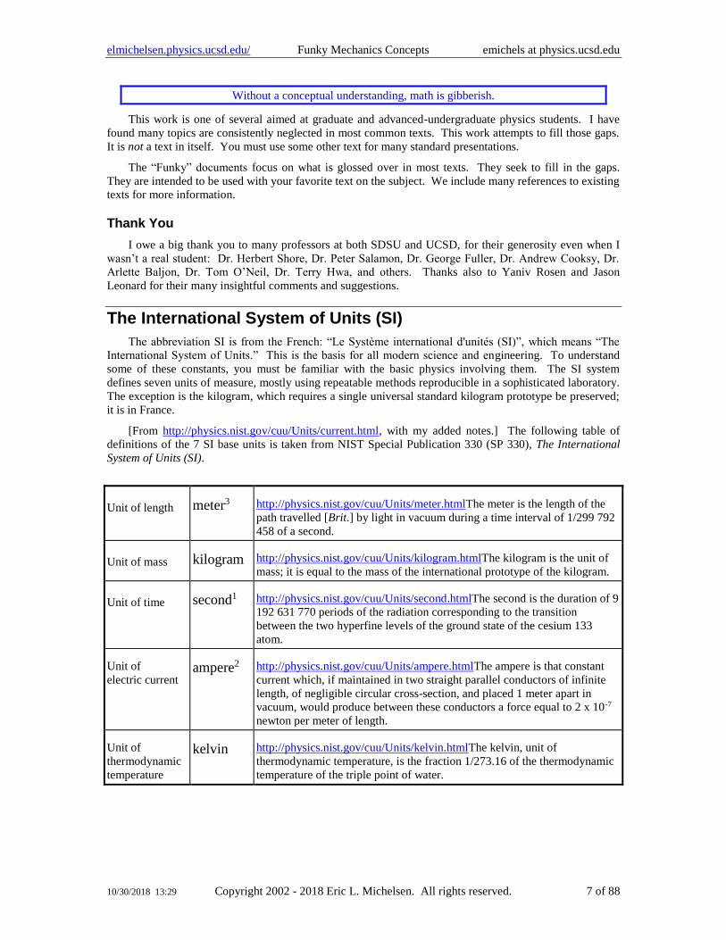
Unit of length meter3 http://physics.nist.gov/cuu/Units/meter.htmlThe meter is the length of the
path travelled [Brit.] by light in vacuum during a time interval of 1/299 792
458 of a second.
Unit of mass kilogram http://physics.nist.gov/cuu/Units/kilogram.htmlThe kilogram is the unit of
mass; it is equal to the mass of the international prototype of the kilogram.
Unit of time second1 http://physics.nist.gov/cuu/Units/second.htmlThe second is the duration of 9
192 631 770 periods of the radiation corresponding to the transition
between the two hyperfine levels of the ground state of the cesium 133
atom.
Unit of
electric current ampere2 http://physics.nist.gov/cuu/Units/ampere.htmlThe ampere is that constant
current which, if maintained in two straight parallel conductors of infinite
length, of negligible circular cross-section, and placed 1 meter apart in
vacuum, would produce between these conductors a force equal to 2 x 10⁻⁷
newton per meter of length.
Unit of
thermodynamic
temperature
kelvin http://physics.nist.gov/cuu/Units/kelvin.htmlThe kelvin, unit of
thermodynamic temperature, is the fraction 1/273.16 of the thermodynamic
temperature of the triple point of water.
elmichelsen.physics.ucsd.edu/ Funky Mechanics Concepts emichels at physics.ucsd.edu
10/30/2018 13:29 Copyright 2002 - 2018 Eric L. Michelsen. All rights reserved. 8 of 88
Unit of
amount of
substance
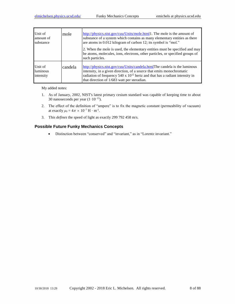
mole http://physics.nist.gov/cuu/Units/mole.html1. The mole is the amount of
substance of a system which contains as many elementary entities as there
are atoms in 0.012 kilogram of carbon 12; its symbol is “mol.”
2. When the mole is used, the elementary entities must be specified and may
be atoms, molecules, ions, electrons, other particles, or specified groups of
such particles.
Unit of
luminous
intensity
candela http://physics.nist.gov/cuu/Units/candela.htmlThe candela is the luminous
intensity, in a given direction, of a source that emits monochromatic
radiation of frequency 540 x 1012 hertz and that has a radiant intensity in
that direction of 1/683 watt per steradian.
My added notes:
1. As of January, 2002, NIST's latest primary cesium standard was capable of keeping time to about
30 nanoseconds per year (1·10–15).
2. The effect of the definition of “ampere” is to fix the magnetic constant (permeability of vacuum)
at exactly μ0 = 4 10–7 H · m-1.
3. This defines the speed of light as exactly 299 792 458 m/s.
Possible Future Funky Mechanics Concepts
• Distinction between “conserved” and “invariant,” as in “Lorentz invariant.”
elmichelsen.physics.ucsd.edu/ Funky Mechanics Concepts emichels at physics.ucsd.edu
10/30/2018 13:29 Copyright 2002 - 2018 Eric L. Michelsen. All rights reserved. 9 of 88
2 Symmetries, Coordinates
Elastic Collisions
This section illustrates how understanding physical principles simplifies a problem, and provides
broadly applicable results. We follow these steps:
1. Pose a problem of general interest
2. Transform it to a simpler problem, using a physical principle
3. Solve the simpler problem
4. Generalize the result to all nonrelativistic frames
5. Generalize to 2D collisions in the COM frame
6. Generalize to relativistic collisions
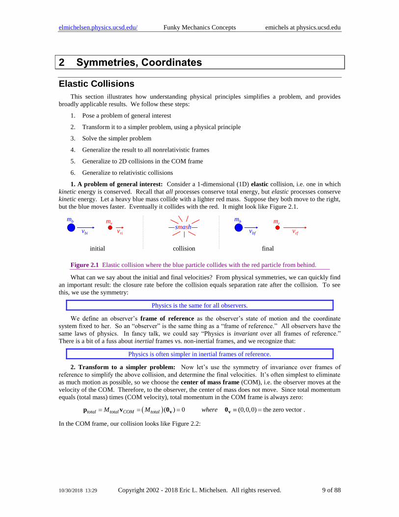
1. A problem of general interest: Consider a 1-dimensional (1D) elastic collision, i.e. one in which
kinetic energy is conserved. Recall that all processes conserve total energy, but elastic processes conserve
kinetic energy. Let a heavy blue mass collide with a lighter red mass. Suppose they both move to the right,
but the blue moves faster. Eventually it collides with the red. It might look like Figure 2.1.
vbi
mb
vri
mrsmash
vbf
mb
vrf
mr
initial collision final
Figure 2.1 Elastic collision where the blue particle collides with the red particle from behind.
What can we say about the initial and final velocities? From physical symmetries, we can quickly find
an important result: the closure rate before the collision equals separation rate after the collision. To see
this, we use the symmetry:
Physics is the same for all observers.
We define an observer’s frame of reference as the observer’s state of motion and the coordinate
system fixed to her. So an “observer” is the same thing as a “frame of reference.” All observers have the
same laws of physics. In fancy talk, we could say “Physics is invariant over all frames of reference.”
There is a bit of a fuss about inertial frames vs. non-inertial frames, and we recognize that:
Physics is often simpler in inertial frames of reference.
2. Transform to a simpler problem: Now let’s use the symmetry of invariance over frames of
reference to simplify the above collision, and determine the final velocities. It’s often simplest to eliminate
as much motion as possible, so we choose the center of mass frame (COM), i.e. the observer moves at the
velocity of the COM. Therefore, to the observer, the center of mass does not move. Since total momentum
equals (total mass) times (COM velocity), total momentum in the COM frame is always zero:
( )( ) 0 (0,0,0) the zero vectortotal total COM totalM M where= = = =v vp v 0 0 .
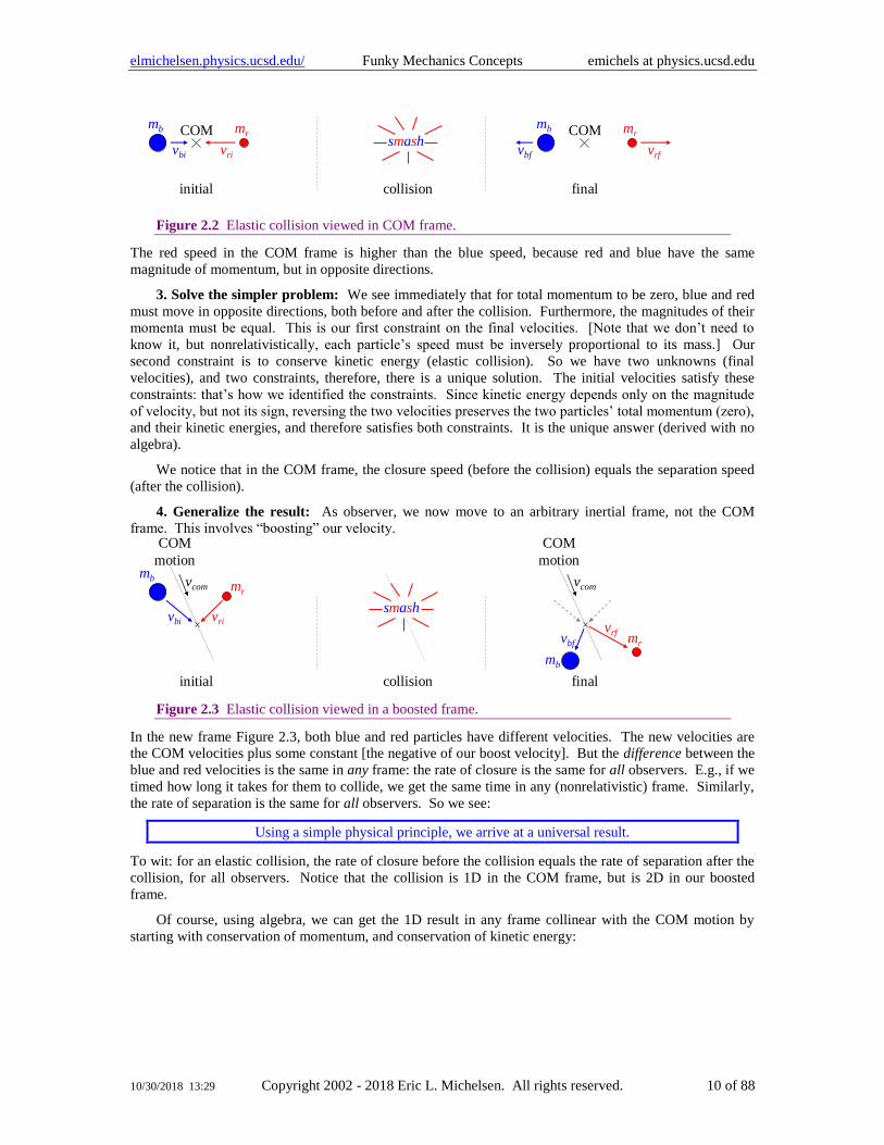
In the COM frame, our collision looks like Figure 2.2:
elmichelsen.physics.ucsd.edu/ Funky Mechanics Concepts emichels at physics.ucsd.edu
10/30/2018 13:29 Copyright 2002 - 2018 Eric L. Michelsen. All rights reserved. 10 of 88
vbi
mb
vri
mrsmash
mb
vrf
mr
initial collision final
vbf
COM COM
Figure 2.2 Elastic collision viewed in COM frame.
The red speed in the COM frame is higher than the blue speed, because red and blue have the same
magnitude of momentum, but in opposite directions.
3. Solve the simpler problem: We see immediately that for total momentum to be zero, blue and red
must move in opposite directions, both before and after the collision. Furthermore, the magnitudes of their
momenta must be equal. This is our first constraint on the final velocities. [Note that we don’t need to
know it, but nonrelativistically, each particle’s speed must be inversely proportional to its mass.] Our
second constraint is to conserve kinetic energy (elastic collision). So we have two unknowns (final
velocities), and two constraints, therefore, there is a unique solution. The initial velocities satisfy these
constraints: that’s how we identified the constraints. Since kinetic energy depends only on the magnitude
of velocity, but not its sign, reversing the two velocities preserves the two particles’ total momentum (zero),
and their kinetic energies, and therefore satisfies both constraints. It is the unique answer (derived with no
algebra).
We notice that in the COM frame, the closure speed (before the collision) equals the separation speed
(after the collision).
4. Generalize the result: As observer, we now move to an arbitrary inertial frame, not the COM
frame. This involves “boosting” our velocity.
vbi
mb
vri
mr
smash
mb
vrfmr
initial collision final
vbf
COM
motion
COM
motion
vcom vcom
Figure 2.3 Elastic collision viewed in a boosted frame.
In the new frame Figure 2.3, both blue and red particles have different velocities. The new velocities are
the COM velocities plus some constant [the negative of our boost velocity]. But the difference between the
blue and red velocities is the same in any frame: the rate of closure is the same for all observers. E.g., if we
timed how long it takes for them to collide, we get the same time in any (nonrelativistic) frame. Similarly,
the rate of separation is the same for all observers. So we see:
Using a simple physical principle, we arrive at a universal result.
To wit: for an elastic collision, the rate of closure before the collision equals the rate of separation after the
collision, for all observers. Notice that the collision is 1D in the COM frame, but is 2D in our boosted
frame.
Of course, using algebra, we can get the 1D result in any frame collinear with the COM motion by
starting with conservation of momentum, and conservation of kinetic energy:
elmichelsen.physics.ucsd.edu/ Funky Mechanics Concepts emichels at physics.ucsd.edu
10/30/2018 13:29 Copyright 2002 - 2018 Eric L. Michelsen. All rights reserved. 11 of 88
( ) ( )
( ) ( )
( )
2 2 2 2 2 2 2 21 1 1 1
2 2 2 2
b bi r ri b bf r rf b bi bf r rf ri
b bi r ri b bf r rf b bi bf r rf ri
b bi bf
m v m v m v m v m v v m v v
m v m v m v m v m v v m v v
m v v
+ = + − = −
+ = + − = −
− ( ) ( )bi bf r rf riv v m v v+ = − ( )rf ri
bi bf rf ri
bi ri rf bf
v v
v v v v
v v v v
+
+ = +
− = −
I find this obtuse, and not very enlightening. We can make it more insightful by labeling the math:
( ) ( )
( ) ( )2 2 22 22221 1 1
22 2
1
2
momentum lost by momentum gained
r ri r rf r rf ri
r ri r rf r
blue by red
energy lost by energy gainedblue by
b bi b
rf
bf b bi bf
b bi b
r
bf b bi bf ri
m v m v m v v
m v m v m v
m v m v m v v
m v m v m v vv
+ = + =
+ = + =
−
− −
−
( )Factoring:
e
b bi
d
bfm v v− ( ) ( )r rf ribi bf m vv vv = −+ ( )
Canceling:
Rearranging:
initial closure final separationrat
bi bf
bi b
rf ri
rf
e rat
ri
fri
e
rf
v v
v v
v v
vv vv
=
=
+
−
++
−
Better, but this is still nowhere near as simple or as general as the result using physical and mathematical
principles, but no algebra.
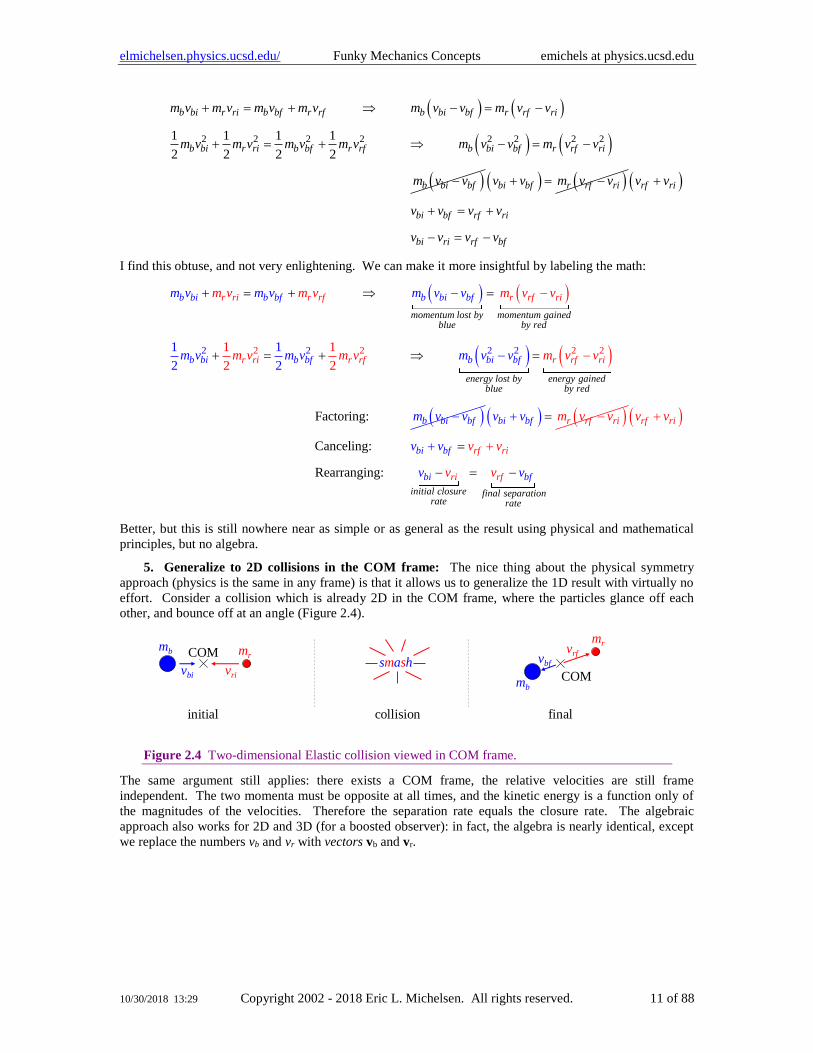
5. Generalize to 2D collisions in the COM frame: The nice thing about the physical symmetry
approach (physics is the same in any frame) is that it allows us to generalize the 1D result with virtually no
effort. Consider a collision which is already 2D in the COM frame, where the particles glance off each
other, and bounce off at an angle (Figure 2.4).
vbi
mb
vri
mrsmash
mb
vrf
mr
initial collision final
vbfCOM
COM
Figure 2.4 Two-dimensional Elastic collision viewed in COM frame.
The same argument still applies: there exists a COM frame, the relative velocities are still frame
independent. The two momenta must be opposite at all times, and the kinetic energy is a function only of
the magnitudes of the velocities. Therefore the separation rate equals the closure rate. The algebraic
approach also works for 2D and 3D (for a boosted observer): in fact, the algebra is nearly identical, except
we replace the numbers vb and vr with vectors vb and vr.
elmichelsen.physics.ucsd.edu/ Funky Mechanics Concepts emichels at physics.ucsd.edu
10/30/2018 13:29 Copyright 2002 - 2018 Eric L. Michelsen. All rights reserved. 12 of 88
6. Generalize to relativistic mechanics: Now here’s the big payoff: what about a relativistic
collision, where the particles move at nearly the speed of light? The diagram is qualitatively the same as
above, but the algebra is much harder, what with 2 2( ) 1/ 1 /v v c − , and all. Most importantly, the
symmetries are similar:
(1) Physics is the same for all observers.
(2) Momentum is parallel to velocity, and kinetic energy depends only on the magnitude of velocity.
Therefore, in the COM frame, reversing the velocities reverses the momenta, and leaves kinetic energies
invariant.
We can see these symmetries from the mathematical forms for relativistic momentum and kinetic
energy:
( ) 2
2 2
1( ) , ( ) 1 , ( )
1 /v m E v mc where v and v
v c = = −
−p v v
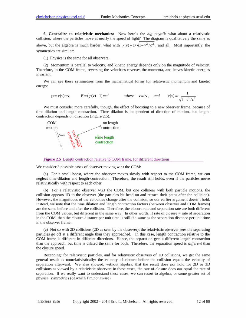
We must consider more carefully, though, the effect of boosting to a new observer frame, because of
time-dilation and length-contraction. Time dilation is independent of direction of motion, but length-
contraction depends on direction (Figure 2.5).
COM
motion
vcom
no length
contraction
max len
gth
contraction
some length
contraction
Figure 2.5 Length contraction relative to COM frame, for different directions.
We consider 3 possible cases of observer moving w.r.t the COM:
(a) For a small boost, where the observer moves slowly with respect to the COM frame, we can
neglect time-dilation and length-contraction. Therefore, the result still holds, even if the particles move
relativistically with respect to each other.
(b) For a relativistic observer w.r.t the COM, but one collinear with both particle motions, the
collision appears 1D to the observer (the particles hit head on and retrace their paths after the collision).
However, the magnitudes of the velocities change after the collision, so our earlier argument doesn’t hold.
Instead, we note that the time dilation and length contraction factors (between observer and COM frames)
are the same before and after the collision. Therefore, the closure rate and separation rate are both different
from the COM values, but different in the same way. In other words, if rate of closure = rate of separation
in the COM, then the closure distance per unit time is still the same as the separation distance per unit time
in the observer frame.
(c) Not so with 2D collisions (2D as seen by the observer): the relativistic observer sees the separating
particles go off at a different angle than they approached. In this case, length contraction relative to the
COM frame is different in different directions. Hence, the separation gets a different length contraction
than the approach, but time is dilated the same for both. Therefore, the separation speed is different than
the closure speed.
Recapping: for relativistic particles, and for relativistic observers of 1D collisions, we get the same
general result as nonrelativistically: the velocity of closure before the collision equals the velocity of
separation afterward. We also showed, without algebra, that the result does not hold for 2D or 3D
collisions as viewed by a relativistic observer: in these cases, the rate of closure does not equal the rate of
separation. If we really want to understand these cases, we can resort to algebra, or some greater set of
physical symmetries (of which I’m not aware).
elmichelsen.physics.ucsd.edu/ Funky Mechanics Concepts emichels at physics.ucsd.edu
10/30/2018 13:29 Copyright 2002 - 2018 Eric L. Michelsen. All rights reserved. 13 of 88
Summary: Using simple physical and mathematical principles, but no algebra, we established the
result that in all cases but one, elastic collisions have a closure rate (before the collision) equal to the
separation rate (after the collision). This is true even relativistically, except for the case where the observer
is relativistic with respect to the COM frame, and the collision appears 2D to the observer. The use of
symmetry saves substantially more algebra in the relativistic case than the nonrelativistic case.
Newton’s Laws
Applicable when v << c, and Δp Δx >> ħ.
Newton’s 3rd Law Isn’t
Isn’t a law, that is. Newton’s 3rd law says that for every force, there is an equal but opposite reaction
force. It implies conservation of momentum:
1 1 2 2 2 1 1 2 1 2 0dp F dt dp F dt F F dp dp and dp dp= = = − = − + =
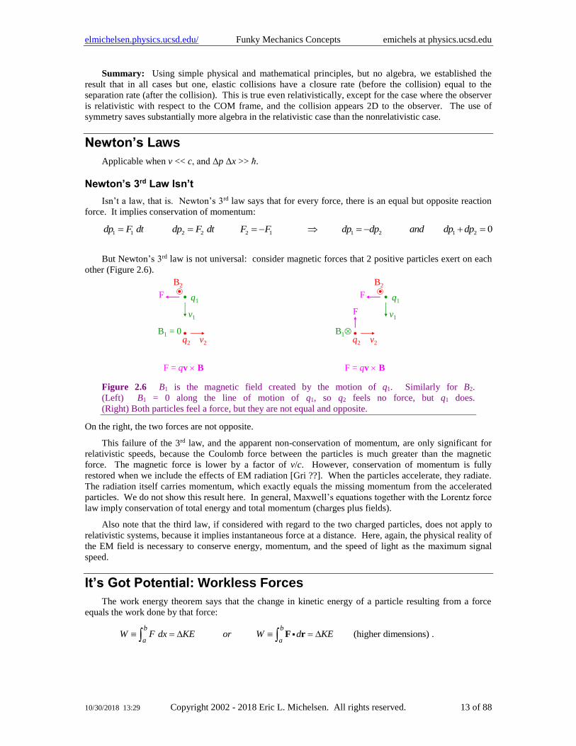
But Newton’s 3rd law is not universal: consider magnetic forces that 2 positive particles exert on each
other (Figure 2.6).
q1
F = qv B
v1
B1 = 0q2 v2
B2
F q1
F = qv B
v1
B1q2 v2
B2
F
F
Figure 2.6 B1 is the magnetic field created by the motion of q1. Similarly for B2.
(Left) B1 = 0 along the line of motion of q1, so q2 feels no force, but q1 does.
(Right) Both particles feel a force, but they are not equal and opposite.
On the right, the two forces are not opposite.
This failure of the 3rd law, and the apparent non-conservation of momentum, are only significant for
relativistic speeds, because the Coulomb force between the particles is much greater than the magnetic
force. The magnetic force is lower by a factor of v/c. However, conservation of momentum is fully
restored when we include the effects of EM radiation [Gri ??]. When the particles accelerate, they radiate.
The radiation itself carries momentum, which exactly equals the missing momentum from the accelerated
particles. We do not show this result here. In general, Maxwell’s equations together with the Lorentz force
law imply conservation of total energy and total momentum (charges plus fields).
Also note that the third law, if considered with regard to the two charged particles, does not apply to
relativistic systems, because it implies instantaneous force at a distance. Here, again, the physical reality of
the EM field is necessary to conserve energy, momentum, and the speed of light as the maximum signal
speed.
It’s Got Potential: Workless Forces
The work energy theorem says that the change in kinetic energy of a particle resulting from a force
equals the work done by that force:
(higher dimensions)b b
a aW F dx KE or W d KE = = F r .
elmichelsen.physics.ucsd.edu/ Funky Mechanics Concepts emichels at physics.ucsd.edu
10/30/2018 13:29 Copyright 2002 - 2018 Eric L. Michelsen. All rights reserved. 14 of 88
The work-energy theorem implies that conservative forces (those whose work between two points is
independent of the path taken between the points) can be written as the (negative) gradient of a scalar
potential:
( ) ( ) (conservative force)F U= −r r ,
where the force is a function of position.
Dissipative forces, friction and drag, are not conservative, and cannot be written with potentials.
On the other hand, workless forces (magnetic and Coriolis forces) always act perpendicular to the
velocity, and thus cannot do work [we neglect the work done by magnetic fields on the intrinsic dipole
moments of fundamental particles such as electrons]. Workless forces can be written as vector potentials:
( ) vector potentialk k where= = F v B v A A .
elmichelsen.physics.ucsd.edu/ Funky Mechanics Concepts emichels at physics.ucsd.edu
10/30/2018 13:29 Copyright 2002 - 2018 Eric L. Michelsen. All rights reserved. 15 of 88
3 Rotating Stuff
Angular Displacements and Angular Velocity Vectors
The following facts underlie the analysis of rotating bodies:
Finite angular displacements are not vectors, but angular velocities are vectors.
In this case, the time derivative of a non-vector is, in fact, a vector. Here’s why:
In 3 or more dimensions, consider rotations about axes fixed in space. Finite angular displacements
(i.e., rotations) are not vectors because adding (composing) two finite angular displacements is not
commutative; the result depends on the order in which the rotations are made. In other words, finite
angular displacements do not commute. (Compare to translational displacements which are vectors:
moving first a meters in x and then b in y yields the same point as first moving b in y and then a in x.)
Therefore, finite angular displacements do not compose a vector space because you cannot decompose a
finite rotation into “component” rotations relative to some basis rotations.
However, infinitesimal angular displacements do commute. Rotating first by dθ from the z-axis, and
then d around the z-axis yields the same rotation as rotating d around the z-axis and then dθ around the y-
axis (i.e., from the z-axis toward the x-axis) (to first order) ??No it doesn’t??. Therefore, infinitesimal
rotations do compose a vector space, and you can decompose any infinitesimal rotation into the
composition of component rotations relative to some basis rotations. We cannot legitimately associate a
vector with a finite rotation. I know, I hear the protests now about “axis of rotation” and finite angles; the
point is that there is no basis into which we can decompose arbitrary finite rotations. The “sum” (i.e.,
composition) of two rotations is not the vector sum of the two rotation “vectors”.
This latter point yields an interesting consequence: whereas finite rotations are not vectors, angular
velocities are vectors. Whereas finite rotations do not compose a vector space, angular velocities do
compose a vector space. This is because angular velocities consist of a large number of infinitesimal
rotations occurring in infinitesimal time periods: dθ/dt, and infinitesimal rotations are vectors.
Furthermore, these results generalize:
For any set of generalized coordinates, even if the {qi} do not compose a vector,
the iq do compose a vector.
Central Forces
Central force problems are widespread in both classical and quantum mechanics. The prototypical
central force is either gravity or electrostatics, where the force is a function of the magnitude of the
separation of the bodies. A central force is a force between 2 bodies which acts along the line of their
separation; it may be attractive or repulsive, and its magnitude depends only on the distance between the
bodies. Two-body problems are especially common, and their solution is greatly simplified by a technique
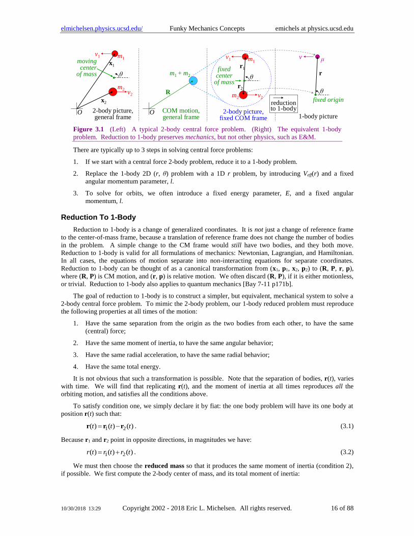
called “reduction to 1-body”. A typical 2-body problem is shown in Figure 3.1, left.
elmichelsen.physics.ucsd.edu/ Funky Mechanics Concepts emichels at physics.ucsd.edu
10/30/2018 13:29 Copyright 2002 - 2018 Eric L. Michelsen. All rights reserved. 16 of 88
v2
fixed center
of mass
v1
2-body picture, fixed COM frame
fixed origin
v
1-body picture
m1
m2
μr1
r
r2
θ
θv2
v1
2-body picture, general frame
m1
m2
x1
x2
θ
O O
R
movingcenter
of mass m1 + m2
COM motion, general frame
reduction to 1-body
Figure 3.1 (Left) A typical 2-body central force problem. (Right) The equivalent 1-body
problem. Reduction to 1-body preserves mechanics, but not other physics, such as E&M.
There are typically up to 3 steps in solving central force problems:
1. If we start with a central force 2-body problem, reduce it to a 1-body problem.
2. Replace the 1-body 2D (r, θ) problem with a 1D r problem, by introducing Veff(r) and a fixed
angular momentum parameter, l.
3. To solve for orbits, we often introduce a fixed energy parameter, E, and a fixed angular
momentum, l.
Reduction To 1-Body
Reduction to 1-body is a change of generalized coordinates. It is not just a change of reference frame
to the center-of-mass frame, because a translation of reference frame does not change the number of bodies
in the problem. A simple change to the CM frame would still have two bodies, and they both move.
Reduction to 1-body is valid for all formulations of mechanics: Newtonian, Lagrangian, and Hamiltonian.
In all cases, the equations of motion separate into non-interacting equations for separate coordinates.
Reduction to 1-body can be thought of as a canonical transformation from (x1, p1, x2, p2) to (R, P, r, p),
where (R, P) is CM motion, and (r, p) is relative motion. We often discard (R, P), if it is either motionless,
or trivial. Reduction to 1-body also applies to quantum mechanics [Bay 7-11 p171b].
The goal of reduction to 1-body is to construct a simpler, but equivalent, mechanical system to solve a
2-body central force problem. To mimic the 2-body problem, our 1-body reduced problem must reproduce
the following properties at all times of the motion:
1. Have the same separation from the origin as the two bodies from each other, to have the same
(central) force;
2. Have the same moment of inertia, to have the same angular behavior;
3. Have the same radial acceleration, to have the same radial behavior;
4. Have the same total energy.
It is not obvious that such a transformation is possible. Note that the separation of bodies, r(t), varies
with time. We will find that replicating r(t), and the moment of inertia at all times reproduces all the
orbiting motion, and satisfies all the conditions above.
To satisfy condition one, we simply declare it by fiat: the one body problem will have its one body at
position r(t) such that:
1 2( ) ( ) ( )t t t= −r r r . (3.1)
Because r1 and r2 point in opposite directions, in magnitudes we have:
1 2( ) ( ) ( )r t r t r t= + . (3.2)
We must then choose the reduced mass so that it produces the same moment of inertia (condition 2),
if possible. We first compute the 2-body center of mass, and its total moment of inertia:
elmichelsen.physics.ucsd.edu/ Funky Mechanics Concepts emichels at physics.ucsd.edu
10/30/2018 13:29 Copyright 2002 - 2018 Eric L. Michelsen. All rights reserved. 17 of 88
11 1 2 2 2 1 1 1
2
2
2 2 2 21 11 1 2 2 1 1 2 1 1 1
2 2
, .
1
mm r m r r r where r etc
m
m mI m r m r m r m r m r
m m
= =
= + = + = +
r
We find the reduced mass which produces this moment of inertia:
2 2
2 2 2 21 1 11 2 1 1 1 1 1
2 2 2
( ) 1 1m m m
I r r r r r r m rm m m
= = + = + = + = +
.
From the last equality, the r12 cancel, and we have:
1 1 1
1 2 1 1 21 1
2 2 1 2 1 2
1 11
m m m m mm m or
m m m m m m
− − − +
= + = = = + +
.
This is excellent, because the reduced mass is independent of r(t), and therefore independent of time. At
this point, we have no more freedom to choose our 1-body parameters. We have satisfied conditions 1 and
2, and must now verify that conditions 3 are 4 are met.
The 2-body radial acceleration is:
12 21 121 2 12 1 2
1 2 2
121 2 12
1 2
1
1 2
1 2 1 2
, , magnitude of force on due to , etc.
1 1( )
1 1
effective
effective
F F Fa a where F m m
m m m
Fa r t a a F
m m m
m mm
m m m m
−
= = =
= + = +
= + = =
+
It’s a miracle! The very same reduced-mass which satisfies the rotational equation, satisfies the radial
equation, as well.
If only the total energy (condition 4) holds up. The potential energy is the same, since it depends only
on radial separation, and we defined that to be the same for 1-body as 2-body. The kinetic energies are:
( )
( )
( )
2
2 2 2 2 2 2 21 12 1 1 2 2 1 1 2 1 1 1
2 2
2 21
222 2 21 2 1 2 1 2
1 2 1 1 11 2 1 2 2 1 2
1 1 11
2 2 2
1. The first term is:
2
1
body
body
m mT m r m r I m r m r I m r I
m m
T r I
m m m m m m mr r r r m r
m m m m m m m
−
−
= + + = + + = + +
= +
= + = + =
+ + +
2
21 2 11 1
2 2
1m m
m rm m
+= +
Lo, and behold! The 1-body energy is the same as the 2-body. All the mechanics is preserved.
Note that the one-body equivalent problem is good for the mechanics only, but not for, say,
electromagnetics. E.g., consider a moving charge near an identical, oppositely moving charge in the
center-of-mass frame.
From E&M, we know the system has no dipole radiation, because the dipole moment is constant:
( )
( ) ( )
1 1 2 2 1 2
1 1 2 2 1 2 1 2
electric charge
But
e e e where e
m m m const const const
= + = +
+ = + = + = =
d r r r r
r r r r r r d
elmichelsen.physics.ucsd.edu/ Funky Mechanics Concepts emichels at physics.ucsd.edu
10/30/2018 13:29 Copyright 2002 - 2018 Eric L. Michelsen. All rights reserved. 18 of 88
However, if we reduce to a 1-body problem, we have a single accelerating charge, but no way to assign a
magnitude to that charge. In fact, there is no charge we can use to reproduce the electromagnetics, because
the 1-body has a varying dipole moment d, which therefore radiates with a dipole component. Hence:
The 1-body reduction is good for mechanics only,
not for other physics, such as electromagnetics.
Also, the reduced system does not reproduce linear motion of R and P, as μ ≠ M ≡ m1 + m2.
To return to the real 2-body motion, we consider Figure 3.1 (right). We can see almost by inspection
that:
2 11 2
1 2 1 2
, andm m
m m m m= + = −
+ +x R r x R r ,
because each body has a distance to the center of mass which is inversely proportional to its mass.
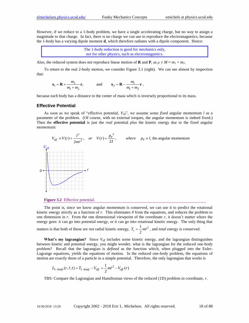
Effective Potential
As soon as we speak of “effective potential, Veff”, we assume some fixed angular momentum l as a
parameter of the problem. (Of course, with no external torques, the angular momentum is indeed fixed.)
Then the effective potential is just the real potential plus the kinetic energy due to the fixed angular
momentum:
22
2( ) , ( ) , , the angular momentum
22eff
plV V r or V r where p l
Imr
+ +
r
Ueff
0
Figure 3.2 Effective potential.
The point is, since we know angular momentum is conserved, we can use it to predict the rotational
kinetic energy strictly as a function of r. This eliminates θ from the equations, and reduces the problem to
one dimension in r. From the one dimensional viewpoint of the coordinate r, it doesn’t matter where the
energy goes: it can go into potential energy, or it can go into rotational kinetic energy. The only thing that
matters is that both of those are not radial kinetic energy, 21
2rT mr= , and total energy is conserved.
What’s my lagrangian? Since Veff includes some kinetic energy, and the lagrangian distinguishes
between kinetic and potential energy, you might wonder, what is the lagrangian for the reduced one-body
problem? Recall that the lagrangian is defined as the function which, when plugged into the Euler-
Lagrange equations, yields the equations of motion. In the reduced one-body problem, the equations of
motion are exactly those of a particle in a simple potential. Therefore, the only lagrangian that works is
21 1
1( , , ) ( )
2body body eff effL r r t T V mr V r− −= − = −
TBS: Compare the Lagrangian and Hamiltonian views of the reduced (1D) problem in coordinate, r.
elmichelsen.physics.ucsd.edu/ Funky Mechanics Concepts emichels at physics.ucsd.edu
10/30/2018 13:29 Copyright 2002 - 2018 Eric L. Michelsen. All rights reserved. 19 of 88
Orbits
To solve for orbits, we must introduce a fixed energy parameter, E, and angular momentum L, as
discussed in the “Reduction to 1-Body” section. TBS. The result is:
( ) , are orbital parameters1 cos
cr where c
=
+.
Other orbital parameters are E, l, a, and b. Any two orbital parameters specifies the “standard” orbit,
defined as having rmin at = 0.
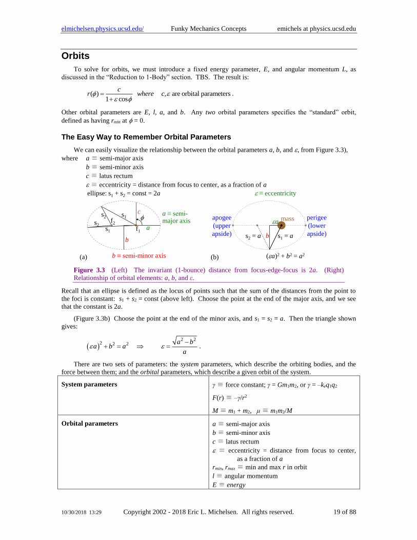
The Easy Way to Remember Orbital Parameters
We can easily visualize the relationship between the orbital parameters a, b, and , from Figure 3.3),
where a ≡ semi-major axis
b ≡ semi-minor axis
c ≡ latus rectum
≡ eccentricity = distance from focus to center, as a fraction of a
f1
f2
s1s2
ellipse: s1 + s2 = const = 2a
a
b
s1
s2
bs2 = a s1 = a
aperigee
(lower
apside)
apogee
(upper
apside)
(a)2 + b2 = a2
massa ≡ semi-major axis
b ≡ semi-minor axis
≡ eccentricity
c
(a) (b)
Figure 3.3 (Left) The invariant (1-bounce) distance from focus-edge-focus is 2a. (Right)
Relationship of orbital elements: a, b, and ε.
Recall that an ellipse is defined as the locus of points such that the sum of the distances from the point to
the foci is constant: s1 + s2 = const (above left). Choose the point at the end of the major axis, and we see
that the constant is 2a.
(Figure 3.3b) Choose the point at the end of the minor axis, and s1 = s2 = a. Then the triangle shown
gives:
( )2 2
2 2 2 a ba b a
a
−+ = = .
There are two sets of parameters: the system parameters, which describe the orbiting bodies, and the
force between them; and the orbital parameters, which describe a given orbit of the system.
System parameters γ ≡ force constant; γ = Gm1m2, or γ = –keq1q2
F(r) ≡ –γ/r2
M ≡ m1 + m2, μ ≡ m1m2/M
Orbital parameters a ≡ semi-major axis
b ≡ semi-minor axis
c ≡ latus rectum
≡ eccentricity = distance from focus to center,
as a fraction of a
rmin, rmax ≡ min and max r in orbit
l ≡ angular momentum
E ≡ energy
elmichelsen.physics.ucsd.edu/ Funky Mechanics Concepts emichels at physics.ucsd.edu
10/30/2018 13:29 Copyright 2002 - 2018 Eric L. Michelsen. All rights reserved. 20 of 88
We start with our fundamental parameters, which we defined in the orbit equation, ( )1 cos
cr
=
+.
By geometric inspection (with no need for dynamics or forces):
min max,1 1
c cr r
= =
+ −.
From the right triangle containing f1f2 and the edge c, and noting that c + hypoteneuse = 2a:
( ) ( ) ( )2 22 21 , from 2 2c a a c c a = − − = + .
As physical quantities, angular momentum and energy must be related to the force constant, γ.
In the standard coordinates ( = 0 to the right), any two orbital parameters fully defines the orbit.
TBS: Kepler’s law about equal areas in equal times results from conservation of angular momentum,
and is true for any central potential, not just 1/r.
Coriolis Acceleration
It turns out that a rotating observer measures two accelerations due to his rotating frame of reference:
(1) centrifugal acceleration, which depends on position, but not velocity, and
(2) Coriolis acceleration, which depends on velocity, but not position.
For now, we call the Coriolis phenomenon an “acceleration” because all masses are accelerated the
same (just like gravity). Therefore, we dispense with calling it a “force,” which would require us to
pointlessly multiply all equations by the accelerated body’s mass.
We first derive the Coriolis acceleration from the body displacement relative to the rotating frame.
Then, for a more complete view, we re-derive it from the viewpoint of a change of velocity in the rotating
frame. We will see that:
The two contributions to Coriolis acceleration are (1) the rotating frame creates a perpendicular
component to the original velocity, and (2) a relative velocity of the rotating reference point. The
effects are equal and additive, resulting in the factor of two in the Coriolis acceleration formula.
Notation: We consider motion in both an inertial frame, and a frame rotating with respect to it. We
use unprimed variables for quantities as measured in the inertial frame, and primed variables for quantities
measured in the rotating frame. Note that the vectors ω and r are the same in both frames, so there is no ω’
or r’.
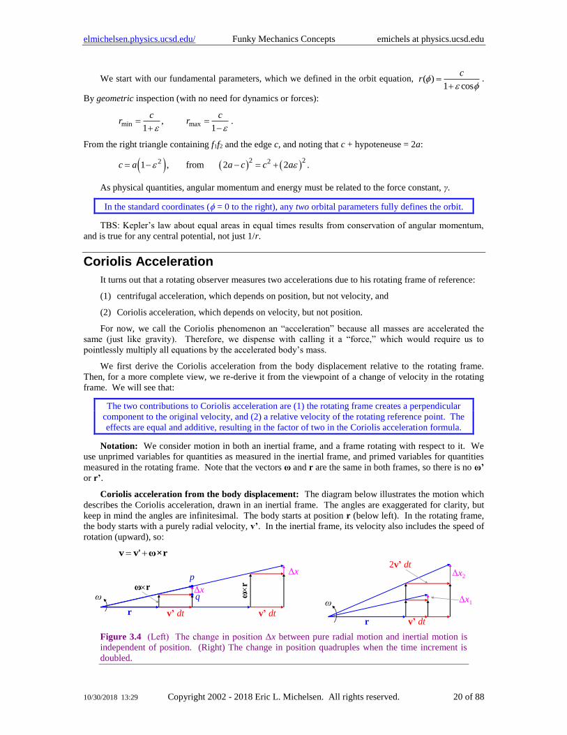
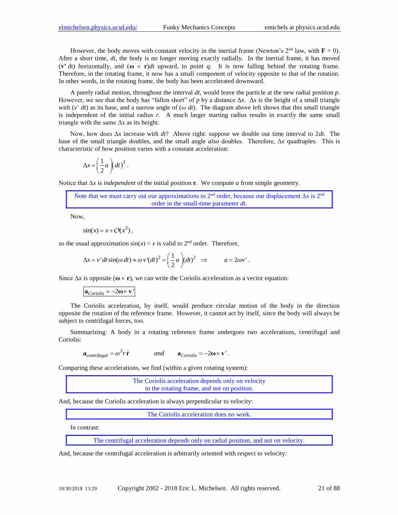
Coriolis acceleration from the body displacement: The diagram below illustrates the motion which
describes the Coriolis acceleration, drawn in an inertial frame. The angles are exaggerated for clarity, but
keep in mind the angles are infinitesimal. The body starts at position r (below left). In the rotating frame,
the body starts with a purely radial velocity, v’. In the inertial frame, its velocity also includes the speed of
rotation (upward), so:
= +v v' ω×r
r v’ dt
ω
Δx2
2v’ dt
Δx1
r v’ dt
ωΔx
Δx
ωr
v’ dt
ω
r
p
q
Figure 3.4 (Left) The change in position Δx between pure radial motion and inertial motion is
independent of position. (Right) The change in position quadruples when the time increment is
doubled.
elmichelsen.physics.ucsd.edu/ Funky Mechanics Concepts emichels at physics.ucsd.edu
10/30/2018 13:29 Copyright 2002 - 2018 Eric L. Michelsen. All rights reserved. 21 of 88
However, the body moves with constant velocity in the inertial frame (Newton’s 2nd law, with F = 0).
After a short time, dt, the body is no longer moving exactly radially. In the inertial frame, it has moved
(v’ dt) horizontally, and (ω r)dt upward, to point q. It is now falling behind the rotating frame.
Therefore, in the rotating frame, it now has a small component of velocity opposite to that of the rotation.
In other words, in the rotating frame, the body has been accelerated downward.
A purely radial motion, throughout the interval dt, would leave the particle at the new radial position p.
However, we see that the body has “fallen short” of p by a distance Δx. Δx is the height of a small triangle
with (v’ dt) as its base, and a narrow angle of (ω dt). The diagram above left shows that this small triangle
is independent of the initial radius r. A much larger starting radius results in exactly the same small
triangle with the same Δx as its height.
Now, how does Δx increase with dt? Above right: suppose we double our time interval to 2dt. The
base of the small triangle doubles, and the small angle also doubles. Therefore, Δx quadruples. This is
characteristic of how position varies with a constant acceleration:
( )21
2x a dt
=
.
Notice that Δx is independent of the initial position r. We compute a from simple geometry.
Note that we must carry out our approximations to 2nd order, because our displacement Δx is 2nd
order in the small-time parameter dt.
Now,
3sin( ) ( )x x x= + ,
so the usual approximation sin(x) ≈ x is valid to 2nd order. Therefore,
2 21' sin( ) '( ) ( ) 2 '
2x v dt dt v dt a dt a v
= = =
.
Since Δx is opposite (ω r), we can write the Coriolis acceleration as a vector equation:
2 'Coriolis = − a ω v
The Coriolis acceleration, by itself, would produce circular motion of the body in the direction
opposite the rotation of the reference frame. However, it cannot act by itself, since the body will always be
subject to centrifugal forces, too.
Summarizing: A body in a rotating reference frame undergoes two accelerations, centrifugal and
Coriolis:
2 ˆ 2 'centrifugal Coriolisr and= = − a r a ω v .
Comparing these accelerations, we find (within a given rotating system):
The Coriolis acceleration depends only on velocity
in the rotating frame, and not on position.
And, because the Coriolis acceleration is always perpendicular to velocity:
The Coriolis acceleration does no work.
In contrast:
The centrifugal acceleration depends only on radial position, and not on velocity.
And, because the centrifugal acceleration is arbitrarily oriented with respect to velocity:
elmichelsen.physics.ucsd.edu/ Funky Mechanics Concepts emichels at physics.ucsd.edu
10/30/2018 13:29 Copyright 2002 - 2018 Eric L. Michelsen. All rights reserved. 22 of 88
The centrifugal acceleration can do work and change the system energy.
Coriolis acceleration from velocity-change: It is instructive to consider the Coriolis acceleration
from the viewpoint of velocities, rather than changes in position. We now re-derive it as such. Since the
Coriolis acceleration is first-order in the velocities, we need keep our approximations only to first order.
r
vω
v’
ωv’⊥
v’ = v
p
vp
ωrp
ω(r + v’ dt)
v’⊥
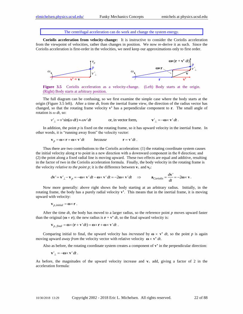
Figure 3.5 Coriolis acceleration as a velocity-change. (Left) Body starts at the origin.
(Right) Body starts at arbitrary position.
The full diagram can be confusing, so we first examine the simple case where the body starts at the
origin (Figure 3.5 left). After a time dt, from the inertial frame view, the direction of the radius vector has
changed, so that the rotating frame velocity v’ has a perpendicular component to r. The small angle of
rotation is ω dt, so:
' 'sin( ) ' or, in vector form, ' 'v v dt v dt dt ⊥ ⊥= = − v ω v .
In addition, the point p is fixed on the rotating frame, so it has upward velocity in the inertial frame. In
other words, it is “running away from” the velocity vector:
' 'p dt because dt= = =v ω r ω v r v .
Thus there are two contributions to the Coriolis acceleration: (1) the rotating coordinate system causes
the initial velocity along r to point in a new direction with a downward component in the θ direction; and
(2) the point along a fixed radial line is moving upward. These two effects are equal and additive, resulting
in the factor of two in the Coriolis acceleration formula. Finally, the body velocity in the rotating frame is
the velocity relative to the point p; it is the difference between v⊥ and vp:
'' ' ' ' 2 ' 2p Coriolis
dd dt dt dt
dt⊥= − = − − = − = = −
vv v v ω v ω v ω v a ω v .
Now more generally: above right shows the body starting at an arbitrary radius. Initially, in the
rotating frame, the body has a purely radial velocity v’. This means that in the inertial frame, it is moving
upward with velocity:
,p initial = v ω r .
After the time dt, the body has moved to a larger radius, so the reference point p moves upward faster
than the original (ω r); the new radius is r + v’ dt, so the final upward velocity is:
, ( ' ) 'p final dt dt= + = + v ω r v ω r ω v .
Comparing initial to final, the upward velocity has increased by ω v’ dt, so the point p is again
moving upward away from the velocity vector with relative velocity ω v’ dt.
Also as before, the rotating coordinate system creates a component of v’ in the perpendicular direction:
' ' dt⊥ = − v ω v .
As before, the magnitudes of the upward velocity increase and v⊥ add, giving a factor of 2 in the
acceleration formula:
elmichelsen.physics.ucsd.edu/ Funky Mechanics Concepts emichels at physics.ucsd.edu
10/30/2018 13:29 Copyright 2002 - 2018 Eric L. Michelsen. All rights reserved. 23 of 88
( ), ,' ' ' ' 2 '
'2
p final p initial
Coriolis
d dt dt dt
d
dt
⊥= − − = − − = −
= = −
v v v v ω v ω v ω v
va ω v
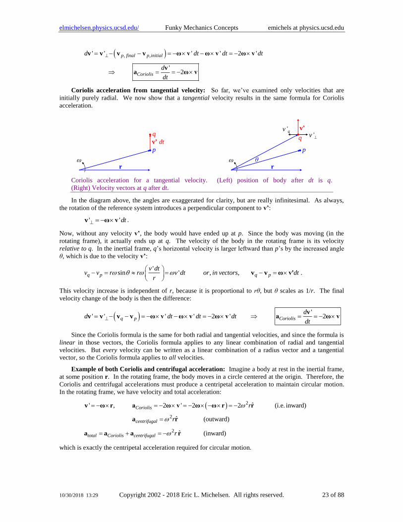
Coriolis acceleration from tangential velocity: So far, we’ve examined only velocities that are
initially purely radial. We now show that a tangential velocity results in the same formula for Coriolis
acceleration.
ωr
p
v’ dt
ω
v’⊥
r
p
v’v’q
θ
Coriolis acceleration for a tangential velocity. (Left) position of body after dt is q.
(Right) Velocity vectors at q after dt.
In the diagram above, the angles are exaggerated for clarity, but are really infinitesimal. As always,
the rotation of the reference system introduces a perpendicular component to v’:
' 'dt⊥ = − v ω v .
Now, without any velocity v’, the body would have ended up at p. Since the body was moving (in the
rotating frame), it actually ends up at q. The velocity of the body in the rotating frame is its velocity
relative to q. In the inertial frame, q’s horizontal velocity is larger leftward than p’s by the increased angle
θ, which is due to the velocity v’:
'sin ' , ,q p q p
v dtv v r r v dt or in vectors dt
r
− = = − =
v v ω v' .
This velocity increase is independent of r, because it is proportional to rθ, but θ scales as 1/r. The final
velocity change of the body is then the difference:
( )'
' ' ' ' 2 ' 2q p Coriolis
dd dt dt dt
dt⊥= − − = − − = − = = −
vv v v v ω v ω v ω v a ω v
Since the Coriolis formula is the same for both radial and tangential velocities, and since the formula is
linear in those vectors, the Coriolis formula applies to any linear combination of radial and tangential
velocities. But every velocity can be written as a linear combination of a radius vector and a tangential
vector, so the Coriolis formula applies to all velocities.
Example of both Coriolis and centrifugal acceleration: Imagine a body at rest in the inertial frame,
at some position r. In the rotating frame, the body moves in a circle centered at the origin. Therefore, the
Coriolis and centrifugal accelerations must produce a centripetal acceleration to maintain circular motion.
In the rotating frame, we have velocity and total acceleration:
( ) 2
2
2
ˆ' , 2 ' 2 2 (i.e. inward)
ˆ (outward)
ˆ (inward)
Coriolis
centrifugal
total Coriolis centrifugal
r
r
r
= − = − = − − = −
=
= + = −
v ω r a ω v ω ω r r
a r
a a a r
which is exactly the centripetal acceleration required for circular motion.
elmichelsen.physics.ucsd.edu/ Funky Mechanics Concepts emichels at physics.ucsd.edu
10/30/2018 13:29 Copyright 2002 - 2018 Eric L. Michelsen. All rights reserved. 24 of 88
Lagrangian for Coriolis Effect
Complicated dynamics problems are often easier to solve with Lagrangian or Hamiltonian mechanics.
In a rotating system, then, one needs a lagrangian for the Coriolis acceleration. The Coriolis acceleration is
always perpendicular to the velocity, just like the magnetic force. Therefore, we derive the Coriolis
lagrangian by analogy with the magnetic force. Since lagrangians produce forces (not accelerations), we
must write the Coriolis effect as a force, by multiplying by the body mass. Also, to agree with the Lorentz
force, we rewrite the Coriolis force as v ω (rather than ω v), giving:
( )
2
Therefore: 2
Coriolis Lorentzm q
m q
= =
F v ω F v B
ω B
In other words:
The angular velocity 2ω acts on a mass
much like a magnetic field acts on a charge.
Therefore, we can construct a Coriolis vector-potential for the vector (2ω), just as we construct a magnetic
vector potential for B:
2
Then
Coriolis
CoriolisL m L q
= =
= =
A ω A B
v A v A
To complete the story for Lagrangian mechanics, we need the potential for the centrifugal force. We
get:
2 2 2
0
( ) 1( ) , ( ) ( )
2
r
centrifugal centrifugal
U rF r m r U r dr F r m r
r
= = − = − = −
.
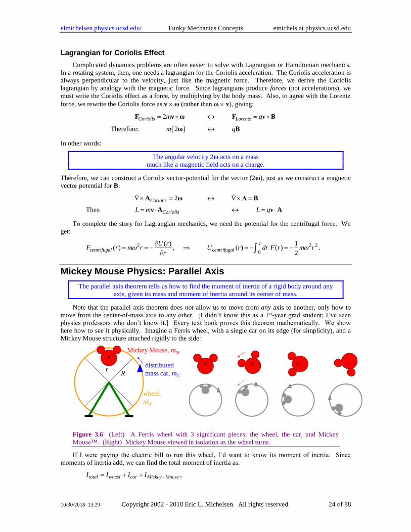
Mickey Mouse Physics: Parallel Axis
The parallel axis theorem tells us how to find the moment of inertia of a rigid body around any
axis, given its mass and moment of inertia around its center of mass.
Note that the parallel axis theorem does not allow us to move from any axis to another, only how to
move from the center-of-mass axis to any other. [I didn’t know this as a 1st-year grad student; I’ve seen
physics professors who don’t know it.] Every text book proves this theorem mathematically. We show
here how to see it physically. Imagine a Ferris wheel, with a single car on its edge (for simplicity), and a
Mickey Mouse structure attached rigidly to the side:
distributed
mass car, mCR
Mickey Mouse, mM
wheel,
mW
r
Figure 3.6 (Left) A Ferris wheel with 3 significant pieces: the wheel, the car, and Mickey
Mouse™. (Right) Mickey Mouse viewed in isolation as the wheel turns.
If I were paying the electric bill to run this wheel, I’d want to know its moment of inertia. Since
moments of inertia add, we can find the total moment of inertia as:
total wheel car Mickey MouseI I I I −= + + ,
elmichelsen.physics.ucsd.edu/ Funky Mechanics Concepts emichels at physics.ucsd.edu
10/30/2018 13:29 Copyright 2002 - 2018 Eric L. Michelsen. All rights reserved. 25 of 88
assuming the spokes are negligible. All the mass of the wheel is at the same radius, R, so we have the
standard formua:
2wheel WI m R= .
As the car goes around the wheel, it remains pointing up, so the occupants are comfortable. That is,
the car itself doesn’t rotate (it just revolves around the wheel center). Therefore, even if the car has a
broadly distributed mass, it is only the center-of-mass motion that matters. Hence, the only rotation of the
car is its rotation around the wheel, and that is the only moment of inertia that contributes to the total:
2car CI m R= .
Mickey is a different story. Mickey Mouse’s center of mass is at radius r. First, his entire mass rotates
in a circle of radius r, much like the car. This “global” rotation certainly contributes to his moment of
inertia:
2Mickey wheel MI m r− = .
In addition, if we look at Mickey’s motion about his center-of-mass, we see that Mickey himself also
rotates around in a circle (Figure 3.6 right). This rotation is simultaneous with, and in addition to, his entire
mass rotating around the wheel. The car does not have this rotation about its center-of-mass. Mickey’s
self-rotation also contributes to the total rotational inertia, exactly the amount of Mickey’s moment of
inertia around his center-of-mass. Therefore, Mickey’s complete moment of inertia is:
2Mickey M Mickey CMI m r I −= + .
But this is just the parallel axis theorem!
The parallel axis theorem simply sums the “global” rotation of an object’s center-of-mass about an
axis, with the object’s “local” rotation about its own center-of-mass.
Note that if Mickey Mouse is indeed made of 3 circles, we can compute his center-of-mass moment of
inertia using, again, the parallel axis theorem on each of the 3 circles.
In unusual cases, we might use the parallel axis theorem in reverse: if we know the moment of inertia
about a non-CM axis, and we know the object’s mass and distance to the CM-axis, we could compute the
moment of inertia about the CM:
2non-CMCMI I mR= − .
Moment of Inertia Tensor: 3D
In 3 dimensions, the instantaneous angular momentum of a rigid body is not necessarily aligned
with the axis of rotation (it is when considering 2D planar rotation).
TBS: How can this be??
The moment of inertia tensor relates the angular velocity to angular momentum:
3
1
i ij j
j
or M I =
= = M Iω (TBS: a real picture of the vectors here).
[In fact, the moment of inertia tensor is a Cartesian tensor, not a true Riemannian tensor, because it involves
finite-displacements of the mass points from the rotation axis.]
elmichelsen.physics.ucsd.edu/ Funky Mechanics Concepts emichels at physics.ucsd.edu
10/30/2018 13:29 Copyright 2002 - 2018 Eric L. Michelsen. All rights reserved. 26 of 88
Rigid Bodies (Rotations)
( )
( )
2 2
2 2 2
2 2
2
Moment of Inertia:
, , : For flat object in : [L&L 32.9+ p100]
Parallel-axis: [F&W26.19 p140, L&L 32.12
ij p ij p pi pj p
p p
i j k z x y
cmij ij ij i j
y z xy xz
I m r x x m xy x z yz
xz yz x y
i j k I I I x y I I I
I I M a a a
+ − −
= − = − + −
− − +
+ − = +
= + −
p101]
( ) ( )
( ) ( )
( ) ( )
1 1 2 3 2 3 1 1 1 1 2 3 2 3
2 2 3 1 3 1 2 2 2 2 3 1 3 1
3 3 1 2 1 2 3 3 3 3 1 2 1 2
Euler eqs: I I I I I I
I I I I I I
I I I I I I
= − = −
= − = −
= − = −
Rotating Frames
Recall that a reference frame is an infinite set of points whose distances to an observer remain
constant. One reference frame may rotate with respect to another reference frame. Frames in which
Newton’s 1st and 2nd laws are obeyed are called inertial frames. If two reference frames are rotating with
respect to each other, then at most one of those frames can be inertial.
We now consider the case of an inertial frame (the “fixed frame”), and a (non-inertial) frame rotating
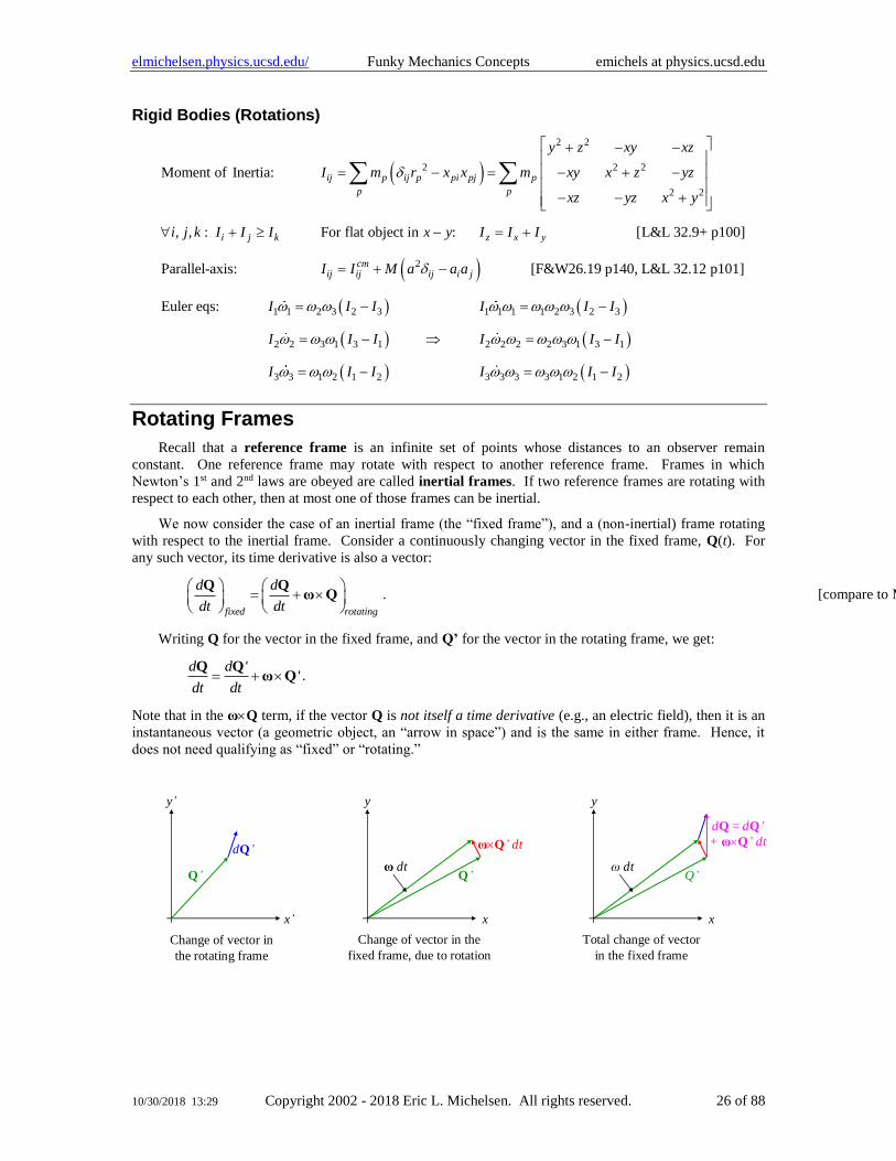
with respect to the inertial frame. Consider a continuously changing vector in the fixed frame, Q(t). For
any such vector, its time derivative is also a vector:
fixed rotating
d d
dt dt
= +
Q Qω Q . [compare to M&T 1st ed 12.7 p 344].
Writing Q for the vector in the fixed frame, and Q’ for the vector in the rotating frame, we get:
''
d d
dt dt= +
Q Qω Q .
Note that in the ωQ term, if the vector Q is not itself a time derivative (e.g., an electric field), then it is an
instantaneous vector (a geometric object, an “arrow in space”) and is the same in either frame. Hence, it
does not need qualifying as “fixed” or “rotating.”
Change of vector in
the rotating frame
y’
x’
Q’
dQ’
Q’
ωQ’ dt
ω dt
Change of vector in the
fixed frame, due to rotation
Total change of vector
in the fixed frame
dQ = dQ’
+ ωQ’ dt
y
x
Q’ω dt
y
x
elmichelsen.physics.ucsd.edu/ Funky Mechanics Concepts emichels at physics.ucsd.edu
10/30/2018 13:29 Copyright 2002 - 2018 Eric L. Michelsen. All rights reserved. 27 of 88
The uncorrected equation in [M&T] is this: fixed rotating
d d
dt dt
= +
Q Qω Q . The problem with this
equation is that the ωQ term is ambiguous: is the Q in this term from the fixed frame or the rotating
frame? [M&T] incorrectly hint that this is irrelevant in all cases, because this is an abstract vector
equation, independent of reference frame. They imply that the ambiguous Q is therefore a vector at an
instant in time (it’s just an arrow in space), and independent of reference frame (as described above). But
this is wrong.
For things like the Coriolis acceleration, Q is itself a time derivative: v = dr/dt, the velocity. There is a
big difference in both magnitude and direction between v, the velocity in the fixed frame, and v’, the
velocity in the rotating frame. In other words, v and v’ are not the same vector written in two different
frames; they are truly different vectors [S&C2 p151b]. The diagram above shows that the component of
acceleration (dQ/dt)fixed due to rotation is ωv’, and not ωv.
Rotating Bodies vs. Rotating Axes
To rotate an axis (say the z axis) to any position requires two parameters, say θ and . To rotate a rigid
body requires 3 parameters, say θ, , and ψ. The reason for the difference is that rotating an axis about
itself produces no change, and is hence unnecessary. For example, consider rotations of a baseball bat with
a label on the side. Starting from anywhere, it takes a θ and rotation to align the axis of the bat to an
arbitrary axis. It then takes a third rotation, ψ, to rotate the label to the desired direction. If the baseball bat
is replaced by an axis, then the last rotation is meaningless; axes have no ψ rotation.
Arbitrary rotations of an axis require two parameters, θ and .
Arbitrary rotations of a rigid body require 3 parameters, θ, , and ψ.
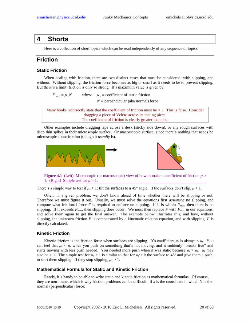
elmichelsen.physics.ucsd.edu/ Funky Mechanics Concepts emichels at physics.ucsd.edu
10/30/2018 13:29 Copyright 2002 - 2018 Eric L. Michelsen. All rights reserved. 28 of 88
4 Shorts
Here is a collection of short topics which can be read independently of any sequence of topics.
Friction
Static Friction
When dealing with friction, there are two distinct cases that must be considered: with slipping, and
without. Without slipping, the friction force becomes as big or small as it needs to be to prevent slipping.
But there’s a limit: friction is only so strong. It’s maximum value is given by
max coefficient of static friction
perpendicular (aka normal) force
s sF N where
N
=
Many books incorrectly state that the coefficient of friction must be < 1. This is false. Consider
dragging a piece of Velcro across its mating piece.
The coefficient of friction is clearly greater than one.
Other examples include dragging tape across a desk (sticky side down), or any rough surfaces with
deep thin spikes in their microscopic surface. Or macroscopic surface, since there’s nothing that needs be
microscopic about friction (though it usually is).
Figure 4.1 (Left) Microscopic (or macroscopic) view of how to make a coefficient of friction μ >
1. (Right) Simple test for μ > 1.
There’s a simple way to test if μs > 1: tilt the surfaces to a 45o angle. If the surfaces don’t slip, μ > 1.
Often, in a given problem, we don’t know ahead of time whether there will be slipping or not.
Therefore we must figure it out. Usually, we must solve the equations first assuming no slipping, and
compute what frictional force F is required to enforce no slipping. If it is within Fmax, then there is no
slipping. If it exceeds Fmax, then slipping does occur. We must then replace F with Fmax in our equations,
and solve them again to get the final answer. The example below illustrates this, and how, without
slipping, the unknown friction F is compensated by a kinematic relation equation, and with slipping, F is
directly calculated.
Kinetic Friction
Kinetic friction is the friction force when surfaces are slipping. It’s coefficient μk is always < μs. You
can feel that μk < μs when you push on something that’s not moving, and it suddenly “breaks free” and
starts moving with less push needed. You needed more push when it was static because μs > μk. μk may
also be > 1. The simple test for μk > 1 is similar to that for μs: tilt the surface to 45o and give them a push,
to start them slipping. If they stop slipping, μk > 1.
Mathematical Formula for Static and Kinetic Friction
Rarely, it’s handy to be able to write static and kinetic friction as mathematical formulas. Of course,
they are non-linear, which is why friction problems can be difficult. If x is the coordinate in which N is the
normal (perpendicular) force:
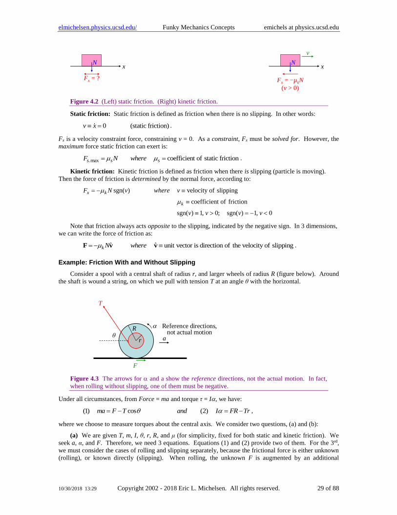
elmichelsen.physics.ucsd.edu/ Funky Mechanics Concepts emichels at physics.ucsd.edu
10/30/2018 13:29 Copyright 2002 - 2018 Eric L. Michelsen. All rights reserved. 29 of 88
xN
Fx = ?
xN
Fx = −µkN
(v > 0)
v
Figure 4.2 (Left) static friction. (Right) kinetic friction.
Static friction: Static friction is defined as friction when there is no slipping. In other words:
0 (static friction)v x = .
Fx is a velocity constraint force, constraining v = 0. As a constraint, Fx must be solved for. However, the
maximum force static friction can exert is:
.max coefficient of static frictions s sF N where = = .
Kinetic friction: Kinetic friction is defined as friction when there is slipping (particle is moving).
Then the force of friction is determined by the normal force, according to:
sgn( ) velocity of slipping
coefficient of friction
sgn( ) 1, 0; sgn( ) 1, 0
x k
k
F N v where v
v v v v
= −
= −
Note that friction always acts opposite to the slipping, indicated by the negative sign. In 3 dimensions,
we can write the force of friction as:
ˆ ˆ unit vector is direction of the velocity of slippingk N where= − F v v .
Example: Friction With and Without Slipping
Consider a spool with a central shaft of radius r, and larger wheels of radius R (figure below). Around
the shaft is wound a string, on which we pull with tension T at an angle θ with the horizontal.
θ a
T
F
r
R Reference directions, not actual motion
Figure 4.3 The arrows for and a show the reference directions, not the actual motion. In fact,
when rolling without slipping, one of them must be negative.
Under all circumstances, from Force = ma and torque τ = I, we have:
(1) cos (2)ma F T and I FR Tr = − = − ,
where we choose to measure torques about the central axis. We consider two questions, (a) and (b):
(a) We are given T, m, I, θ, r, R, and μ (for simplicity, fixed for both static and kinetic friction). We
seek a, α, and F. Therefore, we need 3 equations. Equations (1) and (2) provide two of them. For the 3rd,
we must consider the cases of rolling and slipping separately, because the frictional force is either unknown
(rolling), or known directly (slipping). When rolling, the unknown F is augmented by an additional
elmichelsen.physics.ucsd.edu/ Funky Mechanics Concepts emichels at physics.ucsd.edu
10/30/2018 13:29 Copyright 2002 - 2018 Eric L. Michelsen. All rights reserved. 30 of 88
kinematic constraint equation that relates a and α. The transition from rolling to slipping is given by the
maximum friction equation:
( )max sinF F N mg T = = − .
We will see that for any angle θ, there exist tensions that allow rolling (or at least, no slipping), and higher
tensions that demand slipping.
Case 1: Rolling (really, no slipping)
First, we must assume no slipping, and test our result for consistency at the end. When rolling (or
staying still without slipping), the linear acceleration is related to the angular acceleration by
a R= − ,
and F must be solved for. (We derive the above by considering the instantaneous rotation of the spool
about its point of contact with the ground.) Eliminating first a, then α, from our (1) and (2) yields:
( ) ( )
( )
( )
2 2
2
(3) cos (4) /
cos
cos 1
cos /
1 /
m R F T and I FR Tr FR Tr I
R FR Trm F T
I
mTRr mR F mRT F F
I I I
T mRr IF
mR I
− = − = − → = −
−− = −
+ = + = +
+=
+
If F < Fmax, then our assumption of no slipping is valid. Then, substituting F into (1) and (2) gives a and α.
If not, then we have Case 2: slipping.
Case 2: Slipping
With slipping, a and α are now independent (the kinematic constraint doesn’t apply). But this only
happens when friction is at its maximum, so we find F directly (assuming for simplicity (though
unrealistically) that μs = μk):
( )max sinF F mg T = = − .
We then plug directly into (1) and (2) to solve for a and α.
What if we start with the reverse assumption: assume slipping, and check for consistency? What is
inconsistent if we start by assuming slipping, and there really is no slipping? The friction force will end up
doing more work than the tension puts into the system, and therefore being a source of energy. This is not
possible, but is (in my opinion) harder to check than assuming no slipping, and simply checking if the
required friction force exceeds the maximum available.
(b) If we pull gently enough (T small), there will be no slipping. As we increase T, at some point, the
wheel starts to slip. For given other parameters, at what T does slipping begin?
We start with our equation for F in the case of no slipping from part (a). F is proportional to T, and the
maximum F is
( )max sinF N mg T = = − .
Note that as T increases, the required F for no slipping increases, and also the maximum F decreases.
When the F required for no slipping equals the maximum F, we have the transition tension:
( )1
max 2 2
cos / cos /sin sin
1 / 1 /
mRr I mRr IF mg T T T mg
mR I mR I
−+ +
= − = = + + +
.
elmichelsen.physics.ucsd.edu/ Funky Mechanics Concepts emichels at physics.ucsd.edu
10/30/2018 13:29 Copyright 2002 - 2018 Eric L. Michelsen. All rights reserved. 31 of 88
Rolling Friction
In reality, when something rolls without slipping, there is usually still some energy loss due to the
rolling interface. This loss is called rolling friction, or rolling resistance, or rolling drag. There are several
reasons for this: elastic deformation of the wheels, or the surface beneath them, converts some of the
energy to heat (more so with rubber tires than steel wheels). Imperfections in the circular wheels or flat
surface cause some amount of actual scraping as it rolls. Differences in the wheel sizes on each side of an
axel force some slippage of one or both wheels, which dissipates energy to friction. Imperfections increase
bouncing, and therefore vibration, which carries away energy. Stickiness between the surfaces can also
contribute. The coefficient of rolling friction is typically much less than μk, the coefficient of kinetic
(sliding) friction. The drag force from rolling friction is computed similarly to static and kinetic friction:
coefficient of rolling frictionr rF N where = .
μr for a new car tire is typically ~ 0.01 [en.wikipedia.org/wiki/Rolling_resistance].
Drag
Drag is a kind of friction when a body moves through a fluid (liquid or gas).
Drag differs from kinetic friction in that drag depends on velocity.
Specifically,
2 2ˆ velocity of moving body;a bv where v= − − F v v v v v .
Like most friction, drag acts opposite to the motion.
Damped Harmonic Oscillator
An unforced damped harmonic oscillator has equation of motion:
20 0( ) 2 ( ) ( ) 0 undamped oscillation frequency
damping factor
x t x t x t where
+ + =
This is a linear differential equation with constant coefficients; it’s solutions are therefore exponentials
(possibly complex, which are equivalent to sines and cosines). This section assumes the reader has been
introduced to damped harmonic oscillators, and the method of solving their differential equations.
Since the differential equation is linear, the response of the system to “excitations” (things that make it
move) is linear. The excitations of a system are the initial conditions plus any forcing functions on the
system. In this case, the right hand side is 0, so there are no forcing functions. Therefore, linearity implies:
1 1 1
2 2 2
1 2 1 2 1 2
If (0), (0) produce the response ( )
and (0), (0) produce the response ( )
then (0) (0), (0) (0) produce the response ( ) ( )
x x x t
x x x t
kx x kx x kx t x t+ + +
The solutions to the above equation come in 3 distinct forms, depending on how β compares to ω0.
β < ω0 underdamped: the system oscillates with exponentially decaying amplitude
β = ω0 critically damped: the system decays without oscillation the most rapidly possible
β > ω0 overdamped: the system decays without oscillation
You can think of β < ω0 as “more oscillatory than damped,” so it’s underdamped and oscillates.
Then β > ω0 is “more damped than oscillatory,” so it’s overdamped and doesn’t oscillate.
Sometimes we refer to the damping ratio defined as ζ ≡ β/ω0. Then ζ < 1 is underdamped, ζ = 1 is
critically damped, and ζ > 1 is overdamped.
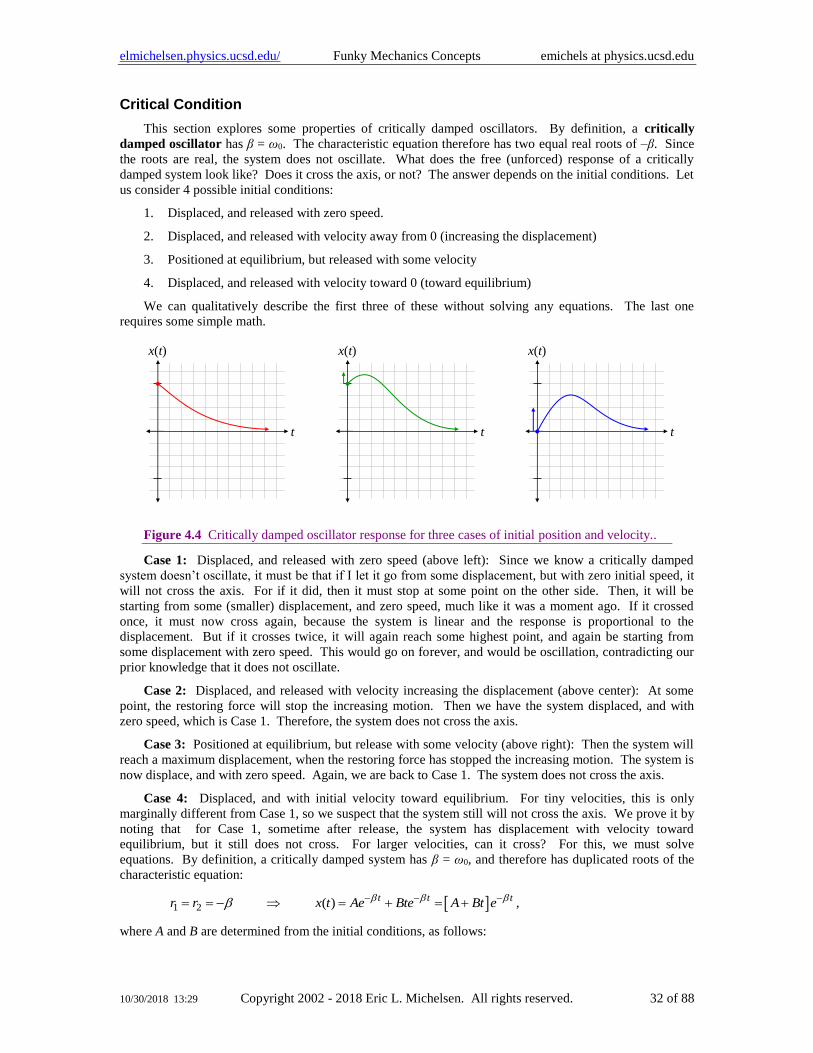
elmichelsen.physics.ucsd.edu/ Funky Mechanics Concepts emichels at physics.ucsd.edu
10/30/2018 13:29 Copyright 2002 - 2018 Eric L. Michelsen. All rights reserved. 32 of 88
Critical Condition
This section explores some properties of critically damped oscillators. By definition, a critically
damped oscillator has β = ω0. The characteristic equation therefore has two equal real roots of –β. Since
the roots are real, the system does not oscillate. What does the free (unforced) response of a critically
damped system look like? Does it cross the axis, or not? The answer depends on the initial conditions. Let
us consider 4 possible initial conditions:
1. Displaced, and released with zero speed.
2. Displaced, and released with velocity away from 0 (increasing the displacement)
3. Positioned at equilibrium, but released with some velocity
4. Displaced, and released with velocity toward 0 (toward equilibrium)
We can qualitatively describe the first three of these without solving any equations. The last one
requires some simple math.
t
x(t)
t
x(t)
t
x(t)
Figure 4.4 Critically damped oscillator response for three cases of initial position and velocity..
Case 1: Displaced, and released with zero speed (above left): Since we know a critically damped
system doesn’t oscillate, it must be that if I let it go from some displacement, but with zero initial speed, it
will not cross the axis. For if it did, then it must stop at some point on the other side. Then, it will be
starting from some (smaller) displacement, and zero speed, much like it was a moment ago. If it crossed
once, it must now cross again, because the system is linear and the response is proportional to the
displacement. But if it crosses twice, it will again reach some highest point, and again be starting from
some displacement with zero speed. This would go on forever, and would be oscillation, contradicting our
prior knowledge that it does not oscillate.
Case 2: Displaced, and released with velocity increasing the displacement (above center): At some
point, the restoring force will stop the increasing motion. Then we have the system displaced, and with
zero speed, which is Case 1. Therefore, the system does not cross the axis.
Case 3: Positioned at equilibrium, but release with some velocity (above right): Then the system will
reach a maximum displacement, when the restoring force has stopped the increasing motion. The system is
now displace, and with zero speed. Again, we are back to Case 1. The system does not cross the axis.
Case 4: Displaced, and with initial velocity toward equilibrium. For tiny velocities, this is only
marginally different from Case 1, so we suspect that the system still will not cross the axis. We prove it by
noting that for Case 1, sometime after release, the system has displacement with velocity toward
equilibrium, but it still does not cross. For larger velocities, can it cross? For this, we must solve
equations. By definition, a critically damped system has β = ω0, and therefore has duplicated roots of the
characteristic equation:
1 2 ( ) t t tr r x t Ae Bte A Bt e − − −= = − = + = + ,
where A and B are determined from the initial conditions, as follows:
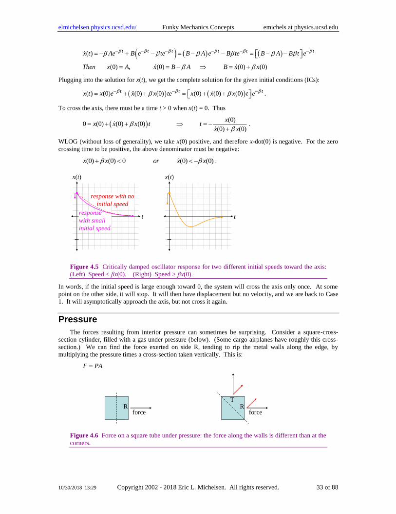
elmichelsen.physics.ucsd.edu/ Funky Mechanics Concepts emichels at physics.ucsd.edu
10/30/2018 13:29 Copyright 2002 - 2018 Eric L. Michelsen. All rights reserved. 33 of 88
( ) ( ) ( )( )
(0) , (0) (0) (0)
t t t t t tx t Ae B e te B A e B te B A B t e
Then x A x B A B x x
− − − − − −= − + − = − − = − −
= = − = +
Plugging into the solution for x(t), we get the complete solution for the given initial conditions (ICs):
( ) ( )( ) (0) (0) (0) (0) (0) (0)t t tx t x e x x te x x x t e − − −= + + = + + .
To cross the axis, there must be a time t > 0 when x(t) = 0. Thus
( )(0)
0 (0) (0) (0)(0) (0)
xx x x t t
x x
= + + = −
+.
WLOG (without loss of generality), we take x(0) positive, and therefore x-dot(0) is negative. For the zero
crossing time to be positive, the above denominator must be negative:
(0) (0) 0 (0) (0)x x or x x + − .
response with no
initial speed
response
with small
initial speed
t
x(t)
t
x(t)
Figure 4.5 Critically damped oscillator response for two different initial speeds toward the axis:
(Left) Speed < βx(0). (Right) Speed > βx(0).
In words, if the initial speed is large enough toward 0, the system will cross the axis only once. At some
point on the other side, it will stop. It will then have displacement but no velocity, and we are back to Case
1. It will asymptotically approach the axis, but not cross it again.
Pressure
The forces resulting from interior pressure can sometimes be surprising. Consider a square-cross-
section cylinder, filled with a gas under pressure (below). (Some cargo airplanes have roughly this cross-
section.) We can find the force exerted on side R, tending to rip the metal walls along the edge, by
multiplying the pressure times a cross-section taken vertically. This is:
F PA=
RT
Rforce force
Figure 4.6 Force on a square tube under pressure: the force along the walls is different than at the
corners.

elmichelsen.physics.ucsd.edu/ Funky Mechanics Concepts emichels at physics.ucsd.edu
10/30/2018 13:29 Copyright 2002 - 2018 Eric L. Michelsen. All rights reserved. 34 of 88
By choosing a different cross-section, though, we get a different answer. The force acting to separate
the cylinder at its corners is different than that acting to rip its walls. If we choose a diagonal (above, right)
as our cross-section, we find the area is larger by √2, and therefore so is the force: F = √2PA.
We can compute this second result a different way, by taking the components of the forces on walls T
and R that lie along the direction of the force acting to separate the cylinder at its corners. Wall T has force
PA, and the component (in red) in the corner-separating direction is (1/√2)PA. But wall R has a similar
component, and adding the two gives the total force, which is again F = √2PA.
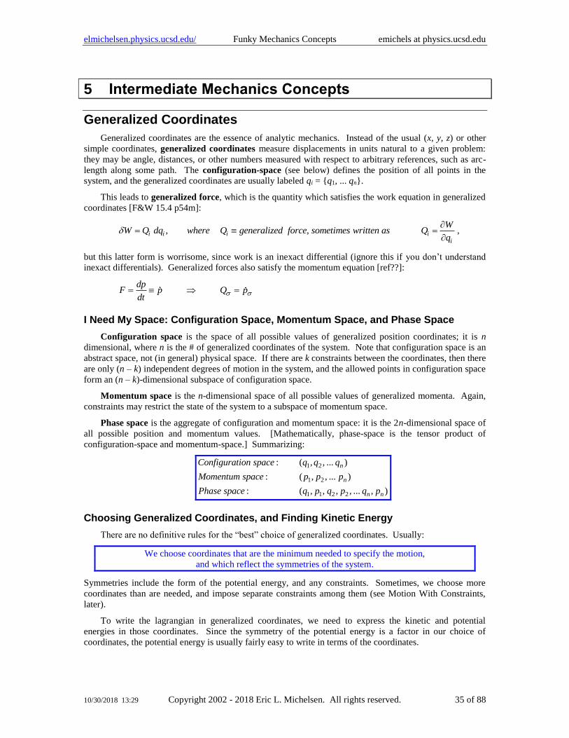
elmichelsen.physics.ucsd.edu/ Funky Mechanics Concepts emichels at physics.ucsd.edu
10/30/2018 13:29 Copyright 2002 - 2018 Eric L. Michelsen. All rights reserved. 35 of 88
5 Intermediate Mechanics Concepts
Generalized Coordinates
Generalized coordinates are the essence of analytic mechanics. Instead of the usual (x, y, z) or other
simple coordinates, generalized coordinates measure displacements in units natural to a given problem:
they may be angle, distances, or other numbers measured with respect to arbitrary references, such as arc-
length along some path. The configuration-space (see below) defines the position of all points in the
system, and the generalized coordinates are usually labeled qi = {q1, ... qn}.
This leads to generalized force, which is the quantity which satisfies the work equation in generalized
coordinates [F&W 15.4 p54m]:
, ,i i i ii
WW Q dq where Q generalized force sometimes written as Q
q
= =
,
but this latter form is worrisome, since work is an inexact differential (ignore this if you don’t understand
inexact differentials). Generalized forces also satisfy the momentum equation [ref??]:
dpF p Q p
dt = =
I Need My Space: Configuration Space, Momentum Space, and Phase Space
Configuration space is the space of all possible values of generalized position coordinates; it is n
dimensional, where n is the # of generalized coordinates of the system. Note that configuration space is an
abstract space, not (in general) physical space. If there are k constraints between the coordinates, then there
are only (n – k) independent degrees of motion in the system, and the allowed points in configuration space
form an (n – k)-dimensional subspace of configuration space.
Momentum space is the n-dimensional space of all possible values of generalized momenta. Again,
constraints may restrict the state of the system to a subspace of momentum space.
Phase space is the aggregate of configuration and momentum space: it is the 2n-dimensional space of
all possible position and momentum values. [Mathematically, phase-space is the tensor product of
configuration-space and momentum-space.] Summarizing:
1 2
1 2
1 1 2 2
: ( , , ... )
: ( , , ... )
: ( , , , , ... , )
n
n
n n
Configuration space q q q
Momentum space p p p
Phase space q p q p q p
Choosing Generalized Coordinates, and Finding Kinetic Energy
There are no definitive rules for the “best” choice of generalized coordinates. Usually:
We choose coordinates that are the minimum needed to specify the motion,
and which reflect the symmetries of the system.
Symmetries include the form of the potential energy, and any constraints. Sometimes, we choose more
coordinates than are needed, and impose separate constraints among them (see Motion With Constraints,
later).
To write the lagrangian in generalized coordinates, we need to express the kinetic and potential
energies in those coordinates. Since the symmetry of the potential energy is a factor in our choice of
coordinates, the potential energy is usually fairly easy to write in terms of the coordinates.
elmichelsen.physics.ucsd.edu/ Funky Mechanics Concepts emichels at physics.ucsd.edu
10/30/2018 13:29 Copyright 2002 - 2018 Eric L. Michelsen. All rights reserved. 36 of 88
However, kinetic energy is often harder. The generalized coordinates might have complicated
relationships to Cartesian coordinates, and they may be time dependent. A very common procedure for
finding the kinetic energy is to write the position of each particle in Cartesian coordinates, as a function of
the generalized coordinates, and possibly time:
( , ) ( , ) ( , )i i ix x q t y y q t z z q t= = =
Then the magnitude of the velocity squared is obtained by taking time derivatives of the Cartesian
coordinates, and summing their squares:
2 2 2 2 2 2 2( , ) ( , ) ( , ) ( , ) ( , ) ( , ) ( , )2
i i i i i i i
mv q t x q t y q t z q t T x q t y q t z q t = + + = + +
A simple example: Let us compute the lagrangian for a simple pendulum, in the generalized
coordinate θ, measured as angular displacement from the vertical. In this case, both kinetic and potential
energy are most easily expressed in Cartesian coordinates x and y. Therefore, we need to convert from θ to
(x, y) for both T and U. [You might wonder, then, “Why didn’t we use (x, y) coordinates in the first place?”
The reason is that using θ requires only one generalized coordinate, whereas using (x, y) requires two
coordinates and a constraint equation. Try it, and you’ll quickly see that (x, y) coordinates are nearly
intractable.] For potential energy, we have:
( , ) ( , ) cos ( ) cosU x y mgy and y Y t l U mgl = = = − = −
For kinetic energy:
( )
( )
( )2 2 2 2 2 2 2 2
( , ) sin , ( , ) cos
( , ) cos ( . ) sin
( , ) ( , ) cos sin2 2 2
x t l x t l
y t l y t l
m m mT x t y t l l
= =
= − =
= + = + =
We see that the final v2 could also have been deduced from the definition of a “radian.” Note that we
frequently need to use trigonometric identities to simplify our final results in terms of our generalized
coordinates. Know your sum and difference angle identities (see Formulas section).
Manifold mathematicians will notice that in computing the kinetic energy, we have actually computed
the metric field for our coordinates. Note that the metric field is only a true tensor in a coordinate basis,
and so the metric computed here is generally not a true tensor field.
D’Alembert’s Principle
[Section under construction.] D’Alembert’s principle is the fundamental principle of analytical
mechanics, according to Cornelius Lanczos’ Variational Principles of Mechanics [Lan p77t]. Lanczos
[Lan ch 3] has an interesting discussion of the progression from Newton’s laws, to d’Alembert’s principle.
D’Alembert’s principle is [equivalent to?? implies??] Hamilton’s principle, and other lesser-known
principles of Euler, Lagrange, and Jacobi. Therefore, it is the “only postulate of analytical mechanics,” as
Lanczos sees it.
D’Alembert’s principle can be integrated with respect to time to get Hamilton’s principle [Lan p11-3].
Hamilton’s principle is valid only when d’Alembert’s principle is valid.
[Lan] points out specifically how action-minimizing principles now describe all fields of physics, far
beyond what Lagrange could have anticipated.
D’Alembert’s principle of virtual work (1742) attempts to “reduce” dynamics problems to “statics.”
Essentially, we rename the rate of change of momentum as a “force”: the inertial force. Then the sum of
all the “forces” equals zero. For example:
elmichelsen.physics.ucsd.edu/ Funky Mechanics Concepts emichels at physics.ucsd.edu
10/30/2018 13:29 Copyright 2002 - 2018 Eric L. Michelsen. All rights reserved. 37 of 88
#
1
0 0,
particles
e i e
i
dm where
dt=
= = → − = = + = = −p
F a F p F F F F p .
This looks like a statics problem. Similarly for rotations, we relate torque and angular momentum:
#
1
0 0,
particles
e i e
i
dI where
dt=
= = → − = = = = −L
T θ T L T+T T T L .
The inertial force originates from the center-of-mass of the system; the inertial torque is a moment, and can
act about any arbitrary point (in fact, it’s the same around all points).
In a static system, the sum of the forces is zero. Therefore, the gradient of the total potential, which is
the sum of the forces, is zero:
0V= − =F .
For a small displacement of the system, the work done to achieve the displacement equals the change in
potential energy, which is simply V·δr:
0 (infinitesimal displacement )W V = = =r F r r .
By calling ma a “force”, we have one form of d’Alembert’s principle: Constraint forces do no work on
virtual displacements. Why??
Like all good variational principles, according to [Lan], d’Alembert’s principle applies to generalized
coordinates, not just rectangular ones. In addition, d’Alembert’s principle applies for both holonomic
(integrable) and non-holonomic constraints, making it more general than Hamilton’s stationary-action
principle. [Liu] disputes this claim.
[Liu] states that d’Alembert’s principle applies to velocity constraints only when the velocity terms of
the constraint equations are homogeneous (of any order) in the velocities. In other words, when we can
write the constraint equations as:
( , , ) ( , ) ( , , ) ( , , ) is homogeneous in thei i i i i i i ig q q t f q t s q q t where s q q t q= + .
This is a very large class of velocity constraints, which covers most practical situations.
Lagrangian Mechanics
Introduction
The importance of Lagrangian physics cannot be overemphasized:
All of modern (microscopic) physics, and much macroscopic physics,
can be described by the principle of stationary-action.
To describe different phenomena, we need only find the right lagrangian.
Lagrangian mechanics simplifies calculations through two principles: (1) generalized coordinates, and (2)
Hamilton’s principle, i.e. the principle of stationary action. Machines, including all rigid bodies, always
incorporate parts that constrain each other’s motion. Such constraints reduce the independent degrees of
freedom from the 3N of N point particles. Generalized coordinates allow specifying the positions of all
parts of a system, i.e. its configuration, usually with a minimum number of coordinates. In some cases,
when additional constraints between coordinates are desirable or necessary, they can usually be included in
the Lagrangian method.
Many people mistakenly believe that Lagrangian mechanics is based on
conservation of energy and/or momentum. Neither of these is true.
elmichelsen.physics.ucsd.edu/ Funky Mechanics Concepts emichels at physics.ucsd.edu
10/30/2018 13:29 Copyright 2002 - 2018 Eric L. Michelsen. All rights reserved. 38 of 88
In fact, for macroscopic systems, Lagrangian mechanics applies equally well to systems that conserve
energy and/or momentum, and those that don’t. Furthermore, Lagrangian mechanics provides simple
methods for determining whether energy or momentum is conserved in a given system, but either way,
Lagrangian mechanics provides the correct equations of motion. Microscopic physics always conserves
energy, because there is no friction, as there is in macroscopic physics. However, some frictional forces
can be added into the general Lagrangian framework, though they do not follow the least-action principle.
In simplest form, Lagrange’s equations can be thought of as the freshman physics concept that rate-of-
change of momentum equals force: dp/dt = F, though extended to generalized coordinates. For non-
relativistic, non-magnetic mechanics:
( , , ) ( ) ( , , )
' : 0 (aka Euler-Lagrange equations)
:
V LL q q t T q V q q t F
q q
d L LLagrange s equations
dt q q
d L LCan be written
dt q q
L d LDefining p p F
q dt q
= − = − =
− =
=
= =
Note that if some of the forces are not included in the lagrangian (such as non-potential forces, e.g.
friction), we can include them on the right hand side of Lagrange’s equations, essentially by using :
# # ##
1 1 1 1
Lagrangian non Lagrangian non Lagrangianforces forces forces forces
i j k k
i j k k
dp L LF F F F
dt t q q
− −
= = = =
= = + − =
.
What is a Lagrangian?
Circular though it may seem,
We define the lagrangian of a system as the function (typically of q, q-dot, and t) which, when put
into the Euler-Lagrange equations, yields the equations of motion of the system.
There is no general method for doing the reverse: finding a lagrangian from the equations of motion
[Gol??]. However, [J&S] develop the lagrangian for a charged particle in a magnetic field by first finding
several conditions such a lagrangian must satisfy, and then one needs only a small amount of “guess and
check” to finish. As we will show, there are infinitely many lagrangians for any system, which all give the
same EOMs. Also, different systems can have the same lagrangian (a hoop rotating flat about a point is the
same as a pendulum in gravity??). (There are some unusual examples where a lagrangian gives the correct
equations of motion, but appears to be the wrong lagrangian [ref??], but we need not address that now.)
Equivalently (and still somewhat circularly), the lagrangian can be defined as the function whose time
integral gives the action of the motion. We will see that:
The value of the lagrangian function is independent of the chosen generalized coordinates, since it
is defined by terms which are coordinate independent.
However, the lagrangian does depend (trivially) on the chosen zero of potential energy.
For example, the nonrelativistic nonmagnetic lagrangian is L = T – V, which is independent of coordinate
choice:
( ), , ( , , ) ( , , ), (general non-relativistic lagrangian)
1,... # coordinates .
i i i i i iL q q t T q q t V q q t
i
= −
=
elmichelsen.physics.ucsd.edu/ Funky Mechanics Concepts emichels at physics.ucsd.edu
10/30/2018 13:29 Copyright 2002 - 2018 Eric L. Michelsen. All rights reserved. 39 of 88
Notice that the equations of motion do not define the lagrangian completely. Firstly, any constant
multiple of a lagrangian produces the same equations of motion. It is important to fix this constant,
because:
The lagrangian for a system comprising subsystems
is the sum of the lagrangians of the subsystems.
For this summation to work, every subsystem must have the same multiplicative constant (more later).
The standard convention is to use a scaling such that the coefficient of the scalar potential V(•) is –1. This
scaling also makes the hamiltonian, derived from the lagrangian, equal to the total energy under a few mild
conditions.
Secondly, the total time derivative of any function can be added to the lagrangian, and produces the
same equations of motion. Conventions are looser here, but all common physics has a well-defined agreed-
upon lagrangian.
Note that we often use the typical lagrangian form of ( ), ,L q q t as representative of most, but not all,
physical problems. If our problem has a lagrangian of this form, then our variations of q (and thus q-dot)
are all the possible variations to make. Hamilton’s principle of stationary action then leads to the typical
Euler-Lagrange equations of motion.
However, some lagrangians include higher derivatives. [Lan] page 59b (bottom) gives a problem for
finding the differential equation resulting from a lagrangian including 2nd derivatives. Pages 70+ gives an
example of a physical elastic system (continuous, though) with U(q(x), q’(x), q’’(x) ) (potential energy)
depending on the 2nd derivative q’’(x).
What Is A Derivative With Respect To A Derivative?
There is a notational shortcut that is universal in mechanics: that of defining the lagrangian as a
function of , , and , whereq q t q is the time derivative of q. Then, we take partial derivatives with respect
to ,L
. There’s no new calculus here; it’s just a shortcut to simplify the notation.
To see this, recall that a lagrangian is a function of 3 variables; let’s call them q, b, and t. Then:
( , , ) , , andL L L
L L q b tq b t
=
are all well-defined.
But it happens that when evaluating the lagrangian L(q, b, t), we will always plug-in q for b. So we don’t
bother introducing the variable b, and just write q everywhere, including in the derivatives. So where q
appears in the lagrangian, it is just an argument of the lagrangian function. However, when considering the
action integral over some path q(t) (actual or variational), the lagrangian reduces to a function of time:
( )
( )2
1
( ), ( ), ( ), which allows us to integrate
( ) ( ), ( ), .t
t
L L q t q t t L t
action S q t dt L q t q t t
=
=
Note that the action is a functional of the trajectory q(t).
Hamilton’s Principle: A Motivated Derivation From F = ma
There is a long-standing, but rarely answered, question: why is Hamilton’s Principle of stationary
action true? Or similarly, how did Hamilton come up with it? Given the context of Hamilton’s time (c.
1834), one can imagine a plausible train of thought leading to Hamilton’s Principle. We motivate and
derive here Hamilton’s principle, starting with a very simple form. Next, we motivate the extension for
magnetic forces. We then describe how the Principle rapidly extends to a broad class of important
dynamics problems, including those with constraints of various forms. This wide application was reason
elmichelsen.physics.ucsd.edu/ Funky Mechanics Concepts emichels at physics.ucsd.edu
10/30/2018 13:29 Copyright 2002 - 2018 Eric L. Michelsen. All rights reserved. 40 of 88
enough to drive the exploration of Hamilton’s Principle that ensued for over a hundred years, so that today,
virtually all of fundamental physics can be given in Lagrangian form. The following derivation also
introduces the power of coordinate-free methods, which are very important in many fields, such as tensor
calculus, differential geometry, and Relativity. [I don’t yet have the derivation of time-dependent
lagrangians.??]
There are two important features of Hamilton’s era: First, outside of classical mechanics, the
mathematical theory of the calculus of variations was already well-known. From the brachistochrone
problem (posed by Leibnitz and Bernooulli in 1696 [Gossick p1]), and others like it, the Euler-Lagrange
(E-L) equations were known to make stationary an integral, with fixed endpoints, of the form:
2
1
1 2 1 2( ( ), '( )) , , ( ), and ( ) are fixedx
xf y x y x dx where x x y x y x . (5.1)
The function, y(x), which makes the integral stationary with respect to small variations in y(x), satisfies the
E-L equation:
( , ') ( , ') 0'
df y y f y y
y dx y
− =
. (5.2)
This is a differential equation in y(x). Therefore, solving this E-L equation finds the y(x) that makes (5.1)
stationary.
Another feature of Hamilton’s day was that there was a long-standing belief that nature was elegant
and parsimonious, i.e. that the laws of nature satisfied minimization properties. For example, as early as c.
60 CE, Hero of Alexandria (Heron) stated a form of Fermat’s principle of least time for light propagation
[Gossick p1]. In the 1700s, Maupertuis believed that the extremal principles of mechanics (those that were
known at the time) proved the existence of God [Gossick p2]. In keeping with this spirit, one might well
ask: Do the laws of motion (classical mechanics) satisfy some minimization principle? Starting directly
with ( )d
F mq p qdt
= = in one dimension, we write:
( ) ( ) 0 is a cartesian coordinate
( ) is derivable from a scalar potential .
dF q p q where q
dt
F q
− =
We recognize this as having the form of the E-L equation (5.2), given the change in notation: y → q, x → t.
Therefore, simple dynamics do, in fact, make stationary some integral:
2
1
( ) makes stationary ( , )t
tq t f q q dt S q .
We now find the function ( , )f q q .
In the notation of dynamics, the E-L equation (5.2) becomes:
( , ) ( , ) 0 ( ), ( ) ( )d d
f q q f q q where q q t q t q tq dt q dt
− = =
. (5.3)
We make this equivalent to ( ) ( ) 0d
F q p qdt
− = by equating corresponding terms:
( ) ( , ), ( ) ( , ) or ( ) ( , )d d
F q f q q p q f q q p q mq f q qq dt dt q q
= = = =
.
We find ( , )f q q , the integrand of the integral that is made stationary against small variations δq(t) and
( )q t , by taking the anti-derivatives (indefinite integrals) of ( ) , andF q dq mq dq :
elmichelsen.physics.ucsd.edu/ Funky Mechanics Concepts emichels at physics.ucsd.edu
10/30/2018 13:29 Copyright 2002 - 2018 Eric L. Michelsen. All rights reserved. 41 of 88
2
( , ) ( ) ( ) a function of ,
1( , ) ( ) a function of .
2
f q q F q dq U q q
f q q mq dq mq T q q
= = − +
= = = +
The constant of integration is irrelevant. Together, these imply:
2
1
( , ) ( ) ( ) and ( , ) is stationaryt
tf q q T q U q f q q dt= − . (5.4)
We rename f( ) to L( ), and call it the lagrangian. We define the integral as S, and call it the action.
This is a most satisfying result, for two reasons: first, f(•) is a scalar function of the motion, and its
value is therefore coordinate-free, though its functional form must depend on the chosen coordinates (more
shortly). Second, f(•) is simply the difference between two well-known and physically meaningful
quantities.
Since the integral is coordinate free, it immediately gives us generalized coordinates: if the integral is
stationary over any small variations in the trajectory q(t), it is stationary over small variations in all
coordinates, even oblique (non-orthogonal) ones. Since stationarity implies the E-L equation [see any
mechanics book ever], the E-L equation is valid in arbitrary coordinates.
We note briefly that any potential energy allows for an arbitrary additive constant; therefore, so does
the lagrangian. This is consistent with the E-L equation containing only derivatives of the lagrangian, so
the E-L equation is insensitive to any additive constant in the lagrangian.
Generalizations of Hamilton’s Principle
Hamilton’s principle in higher dimensions: We have derived Hamilton’s Principle in its simplest
form. We now show that it easily extends to a much wider range of applications. An obvious extension is:
what about 2D or 3D motion? In 3D, starting again with cartesian coordinates, the equations of motion
separate:
{ , , }: ( ) ( ) 0, ( ) ( ) 0, ( ) ( ) 0i x y z x i x y i y z i z
d d dq q q q F q p t F q p t F q p t
dt dt dt − = − = − = .
This leads directly to the straightforward extension of the integrand (5.4). Since the 3 coordinates have
independent motions, minimizing each coordinate’s action individually is equivalent to minimizing their
sum. Therefore, we extend the definition of L to be the sum of the 3 lagrangians from the 3 coordinates.
The action is similarly extended. Skipping some details, this gives:
( ) ( )2
1
#2
1
( )
1( ), ( ) ( ), ( ), ( )
2
i
coordinatest
i i i i i it
i
T q
L q t q t mq U q S L q t q t dt
=
−
.
Again, making the action stationary over small variations in 3D immediately implies the validity of
generalized, oblique 3D coordinates.
We should note that although Hamilton’s principle is valid in 3D, evaluating the kinetic energy T in
oblique coordinates is often difficult, because v2 requires taking a dot-product (or at least, a vector
magnitude). A similar problem appears later when we include magnetics.
Hamilton’s Principle for multiple particles: Another obvious extension is multiple particles. Again,
each can be treated separately at first, and again, minimizing each particle’s individual action is equivalent
to minimizing the total action of the system. Skipping some details, our above definitions of “lagrangian”
and “action” are now valid even when the generalized coordinates span multiple particles.
elmichelsen.physics.ucsd.edu/ Funky Mechanics Concepts emichels at physics.ucsd.edu
10/30/2018 13:29 Copyright 2002 - 2018 Eric L. Michelsen. All rights reserved. 42 of 88
Applying what we’ve learned to the ubiquitous simple harmonic oscillator (SHO), we find that the
action is not necessarily minimized, because the action of SHO motion is not, in fact, a minimum with
respect to variations in q(t), but it is stationary under such variations. This is fine, because the E-L
equations we started with never guaranteed minima in the first place, only that the action integral is
stationary.
Hamilton’s Principle for time varying potentials: What about time-varying potentials? It turns out,
the existing formulas work just as well with them. [I’m not sure how to do this yet?? Perhaps, we apply
our current E-L equations over the infinitesimal interval t1 to t2 ≡ t1 + dt:
2
1
( , , )t
i it
dS L q q t dt .
Over this interval, the explicit time dependence of L can be ignored, and our existing E-L equations are
valid. We’d like to stitch together a large number of such intervals to create a finite interval, but our
current E-L equations only apply when the endpoints at t1 and t2 are fixed. An arbitrary variation δq(t) over
a finite interval would not be fixed at the endpoints of each infinitesimal interval. I’ll bet there’s a way to
fix this, but it’s not obvious to me.]
Hamilton’s Principle for magnetic forces: What about magnetic forces? The Lagrangian formalism
we have developed so far is so powerful, that we are highly motivated to see if we can push it to cover even
more physical situations. Is there a lagrangian that will produce the Lorentz force: F = ev B? While
there is no direct derivation of such a lagrangian, [Jose and Saletan, 1998] point out that, if it exists, it must
be linear in both v and B, and proportional to the charge e. It must also be a scalar, and some kind of
“potential,” so the ansatz ev·A is the minimal lagrangian meeting these criteria. Direct substitution reveals
that this term does, in fact, yield the proper equation of motion (in SI units). The resulting classical
lagrangian, covering many particles in many dimensions (i.e., many degrees of freedom), and magnetism
is:
# particles
1
( , ) ( ) ( ) ( )i i i i j j j
j
L q q T q U q e
=
− + v A r .
Note that both the velocities vj and the dot-products in the last term may be difficult to evaluate in oblique
coordinates.
We also note that since A has gauge freedom, so does the lagrangian. In fact, our lagrangian already
has another “gauge freedom” from early on: adding to the lagrangian the total time derivative of any
function of the coordinates {qi(t)} and time has no effect on the resulting E-L equations of motion. This is
because such a function adds a fixed constant to the action, regardless of the trajectory. Such a constant has
no effect on which trajectories make the action stationary, and so doesn’t affect the equations of motion.
(The gauge function can depend on q(t) and t, but not the coordinate velocities ( )q t , because they are not
fixed at the endpoints of the action integral.)
Other generalizations of Hamilton’s Principle: A development similar to magnetics allows the
inclusion of the Coriolis acceleration when working in a rotating frame of reference. The centrifugal force
is also accommodated by a simple, scalar potential [elsewhere in this work].
Sometimes, it is advantageous to define additional generalized coordinates beyond what we need,
especially if we must compute the forces required to constrain the motion in some way. Such constraints
can be incorporated into Lagrangian mechanics by introducing Lagrange multiplier functions of time, λ(t).
Details are available in standard texts [elsewhere in this work].
Given the success of Lagrangian mechanics in the wide range of applications already described,
physicists are eager to apply its methods to even more situations. For example, can Special Relativity be
described with lagrangian mechanics? As with the magnetic force, one can constrain the possible forms of
such a lagrangian, and a little trial and error reveals that SR can be accommodated. Note, however, that the
relativistic lagrangian is not T – U, even when using the relativistic kinetic energy. (However, the
elmichelsen.physics.ucsd.edu/ Funky Mechanics Concepts emichels at physics.ucsd.edu
10/30/2018 13:29 Copyright 2002 - 2018 Eric L. Michelsen. All rights reserved. 43 of 88
relativistic hamiltonian is the relativistic total energy.] The magnetic lagrangian, just like the Lorentz force
law, is already relativistically valid.
Another big discipline in mechanics is that of deformable continua. Continua have infinite degrees of
freedom, because every point in the “solid” can move. Casting the system in lagrangian form requires
defining generalized coordinates that describe the deformations as functions of both time and space, and
incorporating a new derivative term, the spatial derivative (gradient). The “lagrangian” itself is then built
up from a lagrangian density (essentially “lagrangian per unit volume”):
3( ( , ), ( , ), ( , ), ), and ( , , , )space
q t q t q t t L q q q t d= r r r r .
This form leads naturally to a relativistic scalar definition of the action:
( )2 2
1 1
3 4 ,t t
t t space spacetimeS L dt d dt d where t
= =
r x x r .
With continua and relativistic scalar action now covered, quantum field theory (QFT) becomes
susceptible to yet another generalization of Hamilton’s Principle of stationary action. Furthermore, in a
reach to one of the farthest corners of physics, it turns out that even the Einstein field equations of General
Relativity can be written in lagrangian form.
Hamilton’s Principle is so fundamental and ubiquitous across physics that when a new idea is
formulated, physicists often look early-on for a lagrangian to describe it. Sometimes, journal reviewers
explicitly request a “least-action” formulation [Magueijo, 2003]. Clearly, the principle of stationary action
has grown far beyond anything that William Rowan Hamilton could have imagined back in 1834.
Hamilton’s Principle of Stationary Action: A Variational Principle
We here derive the equations of motion from Hamilton’s Principle, the reverse of what we did above.
(The following notation makes {qi} ≡ q look like a vector. However, the qi are usually not the
components of a vector. For example, polar coordinates are not the components of a vector, because you
can’t add them to find the vector sum. See Funky Mathematical Physics Concepts.) Define q(t) as the set
of position functions: ( )1( ) ( ), ... ( )nt q t q tq . These may describe the actual trajectory of a system through
configuration space, or they may be a hypothetical trajectory. Hamilton’s principle defines the action,
S[q(t)], as a functional of q(t), and states:
For trajectories near the actual trajectory of a system, the variation of the functional S is zero,
i.e., the action is stationary to first order in small variations of the trajectory.
Given the positions of a system at some time, q1(t1), and its positions later, q2(t2), how can we find the
trajectory q(t) of the system between the 2 points? Note that velocities are unknown, even at the endpoints
t1 and t2; solving for q(t) also solves for the velocities everywhere. Hamilton’s principle says the system
trajectory between the two pairs of given points and times makes the action functional stationary between
them:
2
1
( ) makes stationary [ ( )] ( , , )t S t dt L t q
qq q q q .
(Often, q(t) makes the action minimum, but not necessarily.) In other words, the actual trajectory of
motion from q1 to q2 is “shortest” in the sense of being “least action.”
The stationary paths of the action functional S[q(t)] are found by the vanishing of its first order
variation δS[q(t)] for arbitrary infinitesimal variations δq(t) of the path connecting (q1, t1) to (q2, t2). To
compute δS[q(t)], substitute q(t) + δq(t) for q(t) in the definition of action, expand to first order in δq(t),
and integrate the 2nd term by parts (JH 3.38 p 44):
elmichelsen.physics.ucsd.edu/ Funky Mechanics Concepts emichels at physics.ucsd.edu
10/30/2018 13:29 Copyright 2002 - 2018 Eric L. Michelsen. All rights reserved. 44 of 88
2
1
2 2
1 1
1
[ ( )] ( , , ), : ( ) ( )
[ ( )] ( ( ), ( ), ) ( ) ( )( ) ( )
, ...
t
t
t t
t t
n
dS t dt L t NB t t
dt
L LS t dt L t t t dt t t
t t
whereq q
= =
= = +
=
q
q q q q q
q q q q qq q
q
Now we integrate by parts to eliminate δq-dot in favor of δq, noting that δq(t1) = δq(t2) = 0v:
22
11
:
, ( ) , ( )( ) ( )
[ ( )] ( ) ( )( ) ( ) ( )
tt
tt
IBP U dV V dU
L d LLet U dV t dt dU dt V t
t dt t
L d L LS t dt t t
t dt t t
→ −
= = = =
= − +
q qq q
q q qq q q
0( ) ( )
d L L
dt t t
− =
q q
This can be thought of as a generalized Newton’s 2nd law: “rate of change of momentum = sum of forces.”
This equation is Lagrange’s Equation of Motion (LEM), or just Lagrange’s Equation.
Note that since the small variations of the trajectory are arbitrary, the q(t) can be arbitrary generalized
coordinates, so long as they fully specify the positions over time of all degrees of freedom of the system.
In other words:
Hamilton’s principle implies that for any generalized coordinates,
Lagrange’s equations solve for the motion.
Hamilton’s Principle: Why Isn’t “Stationary Action” an Oxymoron?
What is the significance of “least action” vs “stationary action”?
The action for the motion of a system is stationary: either minimum, or non-decreasing.
Action is not necessarily minimized, and it is never maximized [Ref??]. A stationary action might be
neither a minimum nor a maximum. All minima and maxima are stationary paths, but not all stationary
paths are minima or maxima. [Note that some references use the term “extremize” nonstandardly to mean
“make stationary.” Similarly, they may use the term “extremum” nonstandardly to mean “stationary
path.”]
To illustrate, let’s recall a simpler case: a stationary point of a function: In calculus, a function can
have a zero derivative in 3 cases: a maximum, a minimum, or an inflection point. Zero derivative is where
the function is “stationary”: there is no (first-order) change in the function for tiny changes in its argument,
i.e.,
2when '( ) 0 : ( ) ( ) ( )f x f x dx f x O dx= + = + .
E.g., f(x) = x3 has zero derivative at x = 0, but that is neither a maximum nor a minimum. It is an inflection
point.
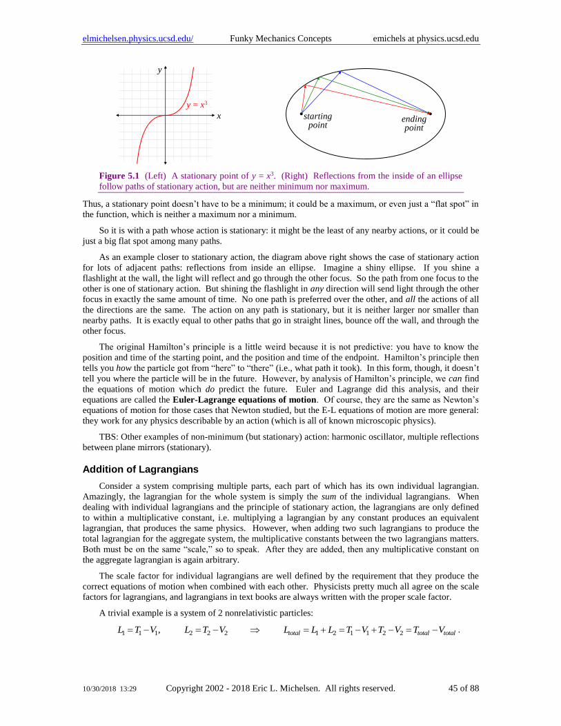
elmichelsen.physics.ucsd.edu/ Funky Mechanics Concepts emichels at physics.ucsd.edu
10/30/2018 13:29 Copyright 2002 - 2018 Eric L. Michelsen. All rights reserved. 45 of 88
x
y
y = x3
starting point
ending point
Figure 5.1 (Left) A stationary point of y = x3. (Right) Reflections from the inside of an ellipse
follow paths of stationary action, but are neither minimum nor maximum.
Thus, a stationary point doesn’t have to be a minimum; it could be a maximum, or even just a “flat spot” in
the function, which is neither a maximum nor a minimum.
So it is with a path whose action is stationary: it might be the least of any nearby actions, or it could be
just a big flat spot among many paths.
As an example closer to stationary action, the diagram above right shows the case of stationary action
for lots of adjacent paths: reflections from inside an ellipse. Imagine a shiny ellipse. If you shine a
flashlight at the wall, the light will reflect and go through the other focus. So the path from one focus to the
other is one of stationary action. But shining the flashlight in any direction will send light through the other
focus in exactly the same amount of time. No one path is preferred over the other, and all the actions of all
the directions are the same. The action on any path is stationary, but it is neither larger nor smaller than
nearby paths. It is exactly equal to other paths that go in straight lines, bounce off the wall, and through the
other focus.
The original Hamilton’s principle is a little weird because it is not predictive: you have to know the
position and time of the starting point, and the position and time of the endpoint. Hamilton’s principle then
tells you how the particle got from “here” to “there” (i.e., what path it took). In this form, though, it doesn’t
tell you where the particle will be in the future. However, by analysis of Hamilton’s principle, we can find
the equations of motion which do predict the future. Euler and Lagrange did this analysis, and their
equations are called the Euler-Lagrange equations of motion. Of course, they are the same as Newton’s
equations of motion for those cases that Newton studied, but the E-L equations of motion are more general:
they work for any physics describable by an action (which is all of known microscopic physics).
TBS: Other examples of non-minimum (but stationary) action: harmonic oscillator, multiple reflections
between plane mirrors (stationary).
Addition of Lagrangians
Consider a system comprising multiple parts, each part of which has its own individual lagrangian.
Amazingly, the lagrangian for the whole system is simply the sum of the individual lagrangians. When
dealing with individual lagrangians and the principle of stationary action, the lagrangians are only defined
to within a multiplicative constant, i.e. multiplying a lagrangian by any constant produces an equivalent
lagrangian, that produces the same physics. However, when adding two such lagrangians to produce the
total lagrangian for the aggregate system, the multiplicative constants between the two lagrangians matters.
Both must be on the same “scale,” so to speak. After they are added, then any multiplicative constant on
the aggregate lagrangian is again arbitrary.
The scale factor for individual lagrangians are well defined by the requirement that they produce the
correct equations of motion when combined with each other. Physicists pretty much all agree on the scale
factors for lagrangians, and lagrangians in text books are always written with the proper scale factor.
A trivial example is a system of 2 nonrelativistic particles:
1 1 1 2 2 2 1 2 1 1 2 2, total total totalL T V L T V L L L T V T V T V= − = − = + = − + − = − .
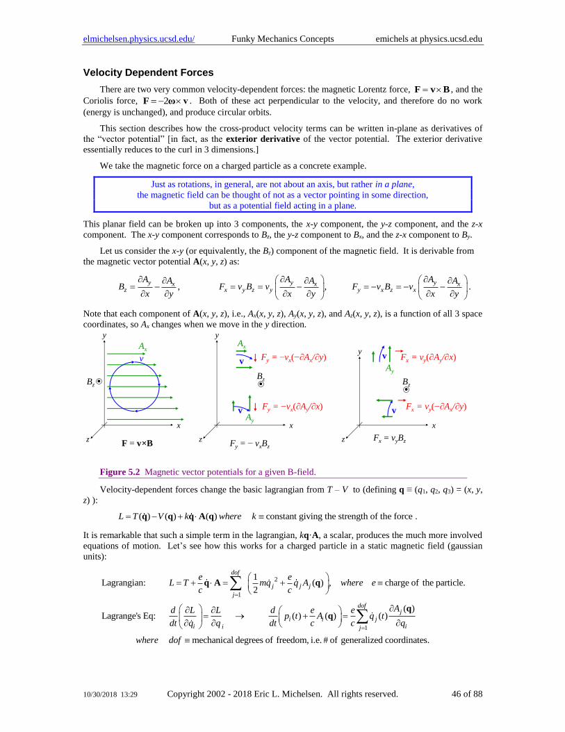
elmichelsen.physics.ucsd.edu/ Funky Mechanics Concepts emichels at physics.ucsd.edu
10/30/2018 13:29 Copyright 2002 - 2018 Eric L. Michelsen. All rights reserved. 46 of 88
Velocity Dependent Forces
There are two very common velocity-dependent forces: the magnetic Lorentz force, = F v B , and the
Coriolis force, 2= − F ω v . Both of these act perpendicular to the velocity, and therefore do no work
(energy is unchanged), and produce circular orbits.
This section describes how the cross-product velocity terms can be written in-plane as derivatives of
the “vector potential” [in fact, as the exterior derivative of the vector potential. The exterior derivative
essentially reduces to the curl in 3 dimensions.]
We take the magnetic force on a charged particle as a concrete example.
Just as rotations, in general, are not about an axis, but rather in a plane,
the magnetic field can be thought of not as a vector pointing in some direction,
but as a potential field acting in a plane.
This planar field can be broken up into 3 components, the x-y component, the y-z component, and the z-x
component. The x-y component corresponds to Bz, the y-z component to Bx, and the z-x component to By.
Let us consider the x-y (or equivalently, the Bz) component of the magnetic field. It is derivable from
the magnetic vector potential A(x, y, z) as:
, ,y y yx x x
z x y z y y x z x
A A AA A AB F v B v F v B v
x y x y x y
= − = = − = − = − −
.
Note that each component of A(x, y, z), i.e., Ax(x, y, z), Ay(x, y, z), and Az(x, y, z), is a function of all 3 space
coordinates, so Ax changes when we move in the y direction.
Fy = − vxBz
y
x
y
x
z
Bz
v
Bz
Fx = vy(−∂Ax/∂y)Fy = −vx(∂Ay/∂x)
Ay
Ax
Fy = −vx(−∂Ax/∂y)
Fx = vyBzz
Fx = vy(∂Ay/∂x)
Ay
F = v×B
y
x
z
Bz
v
Ax
v
vv
Figure 5.2 Magnetic vector potentials for a given B-field.
Velocity-dependent forces change the basic lagrangian from T – V to (defining q ≡ (q1, q2, q3) = (x, y,
z) ):
( ) ( ) ( ) constant giving the strength of the forceL T V k where k= − + q q q A q .
It is remarkable that such a simple term in the lagrangian, kq·A, a scalar, produces the much more involved
equations of motion. Let’s see how this works for a charged particle in a static magnetic field (gaussian
units):
2
1
1
1Lagrangian: ( ) , charge of the particle.
2
( )Lagrange's Eq: ( ) ( ) ( )
mechanical degrees of fre
dof
j j j
j
dofj
i i ji ii j
e eL T mq q A where e
c c
Ad L L d e ep t A q t
dt q q dt c c q
where dof
=
=
= + = +
= → + =
q A q
edom, i.e. # of generalized coordinates.
elmichelsen.physics.ucsd.edu/ Funky Mechanics Concepts emichels at physics.ucsd.edu
10/30/2018 13:29 Copyright 2002 - 2018 Eric L. Michelsen. All rights reserved. 47 of 88
[Note that it is not convenient to write these equations of motion in vector form, because the right hand side
is awkward in vector notation.] These are the equations of motion, so dA/dt (in the last equation) is a result
of the particle moving in space, not because A(r) is changing in time:
( ) ( )
1 1
1 1
1
Define ( ) ( ) ( ) ( )
( )( ) ( ) ( )Then ( )
( )( )Eqs of motion: ( ) ( )
( ) ( )( )
i i
dof dofji i i
jj jj j
dof dofji i
j jj ij j
dofji i
ji jj
t t A t A t
dq tdA t A Aq t
dt dt q q
Adp Ae eq t q t
dt c q c q
Adp Aeq t
dt c q q
= =
= =
=
= =
+ =
= −
A A q q
q q
q q ( ) ( ): .
j i
i j
A ANB
q q
−
q qA
In words, /L q on the left removes q and leaves A(q). Then the d/dt turns A(q) into q A . On the
right, the ∂L/∂q leave the q alone, and acts on A(q) to also produce q ∂A/∂qi terms. These terms from the
left and right combine to produce the “curl” of A.
The last term cancels the j = i term from the sum, so that force in the i direction involves velocities in
all directions except i. But from the point of view of planes instead of directions, we say that the Lorentz
force in the x-y plane is completely determined by the x-y components of the vector potential A. This is the
true nature of the magnetic field:
The magnetic forces in a plane are completely
determined by the vector potential components in that plane.
In traditional terms, the x-y components of A completely determine Bz, but then (for a given velocity in
the x-y plane) the Lorentz force e
c= F v B in the x-y plane is determined completely by Bz. Therefore,
the Lorentz force in the x-y plane is determined completely by the x-y components of A. In other words,
potentials in the plane, stay in the plane.
We’ve now broken the magnetic forces into planes, instead of vectors. But we must remember that
each direction in space is a member of two planes: x is included in the x-y plane and the z-x plane, and
similarly for y and z. Therefore, the x-component of force is the sum of the forces from the x-y plane and
the z-x plane. This is why the force in the x direction involves velocities in both the y and z directions.
Coriolis forces can similarly be taken account by introducing a Coriolis vector potential. See Funky
Electromagnetic Concepts for discussions of finding the vector potential for a given magnetic field (or
other velocity-dependent force). You can use the analogy
2 , , 2Coriolis Lorentz
properties ofthe particle
e eF m F so m and
c c= = v ω v B ω B .
Non-potential Forces
Some forces (e.g., static or kinetic friction, viscous drag) cannot be derived from a potential function
(they are “polygenic forces” in Lanczos’ terminology). Such forces can be incorporated into Lagrange’s
equations by simply writing them on the RHS [Gol p23]:
elmichelsen.physics.ucsd.edu/ Funky Mechanics Concepts emichels at physics.ucsd.edu
10/30/2018 13:29 Copyright 2002 - 2018 Eric L. Michelsen. All rights reserved. 48 of 88
( ), ( ) are the non-potential-derivable forcesi ii i
L d LQ t where Q t
q dt q
− =
.
Examples TBS: kinetic friction, viscous friction. Friction work function of [F&W].
Lagrangians for Relativistic Mechanics
At relativistic speeds, the lagrangian is not T – V (see Funky Relativity Concepts for more information).
The relativistic lagrangian for a charged particle is (in Gaussian units):
2 2 2( , ) 1 / ( ) [LL216.4 p48]
charge of particle, ( ) potential of particle ( ) for an electric field
eL mc v c V
c
where e V e
= − − + −
=
q v v A q
q q
Fully Functional
The concept of functionals is too often glossed over so quickly that it makes no sense. With a few
simple definitions and examples, functionals and functional derivatives are readily understood. This
provides a solid foundation for their use in continuum materials (strings, magnets, fluids, etc.), and in
theoretical analysis, such as classical mechanics. This section requires only simple calculus. We follow
this course:
• Definition of a functional, with examples.
• Functional derivatives, with examples.
• Superposition of small variations, i.e. linearity of functional derivatives.
• A slightly different view of functionals as functions of an infinite number of arguments.
• Sample application: classical mechanics and Euler-Lagrange equations.
A functional takes a function as input and produces a number from it. [Contrast with a function,
which takes a number (or a set of them) and produces a number.] A simple functional might be:
1
0[ ( )] ( )W f x f x dx= .
Square brackets around the function-argument is standard notation for a functional. One of the best known
functionals in physics is the action functional, S[ ]; it acts on the lagrangian, and produces the action, S (a
number):
2
1
( ) ( )t
tS L t L t dt .
However, the lagrangian is a function of the coordinates and velocities, q(t) and ( )q t , which are themselves
functions of time. Therefore, the action can be considered a functional of the coordinates and their
velocities:
( )2
1
( ), ( ) ( ), ( ),t
tS q t q t L q t q t t dt .
Even though q(t) and ( )q t are related, they are treated as independent variables, because there is
so much flexibility in their values that they are, for most practical purposes, independent.
We’ll return to this point when we discuss functional derivatives.
Another example of a functional is the hamiltonian of a continuous medium, such as a string or the
magnetization of a material.
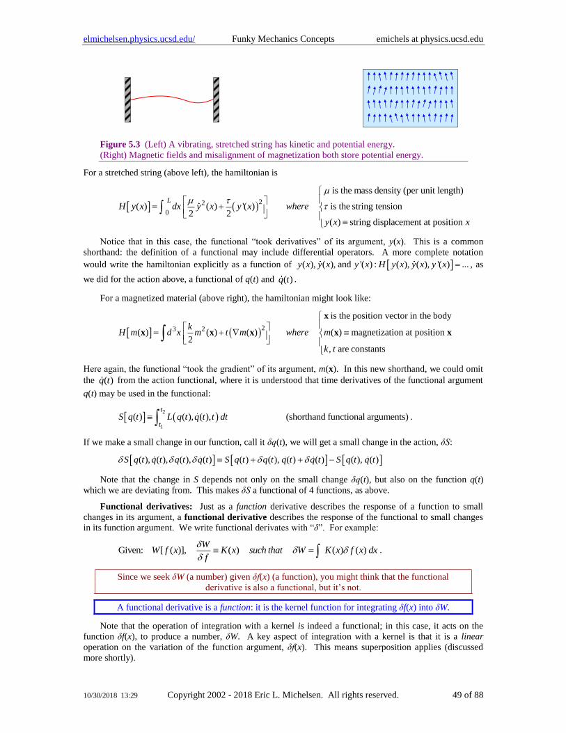
elmichelsen.physics.ucsd.edu/ Funky Mechanics Concepts emichels at physics.ucsd.edu
10/30/2018 13:29 Copyright 2002 - 2018 Eric L. Michelsen. All rights reserved. 49 of 88
Figure 5.3 (Left) A vibrating, stretched string has kinetic and potential energy.
(Right) Magnetic fields and misalignment of magnetization both store potential energy.
For a stretched string (above left), the hamiltonian is
( )22
0
is the mass density (per unit length)
( ) ( ) '( ) is the string tension2 2
( ) string displacement at position
LH y x dx y x y x where
y x x
= +
Notice that in this case, the functional “took derivatives” of its argument, y(x). This is a common
shorthand: the definition of a functional may include differential operators. A more complete notation
would write the hamiltonian explicitly as a function of ( ), ( ), and '( ) : ( ), ( ), '( ) ...y x y x y x H y x y x y x = , as
we did for the action above, a functional of q(t) and ( )q t .
For a magnetized material (above right), the hamiltonian might look like:
( )23 2
is the position vector in the body
( ) ( ) ( ) ( ) magnetization at position2
, are constants
kH m d x m t m where m
k t
= +
x
x x x x x
Here again, the functional “took the gradient” of its argument, m(x). In this new shorthand, we could omit
the ( )q t from the action functional, where it is understood that time derivatives of the functional argument
q(t) may be used in the functional:
( )2
1
( ) ( ), ( ), (shorthand functional arguments)t
tS q t L q t q t t dt .
If we make a small change in our function, call it δq(t), we will get a small change in the action, δS:
( ), ( ), ( ), ( ) ( ) ( ), ( ) ( ) ( ), ( )S q t q t q t q t S q t q t q t q t S q t q t + + −
Note that the change in S depends not only on the small change δq(t), but also on the function q(t)
which we are deviating from. This makes δS a functional of 4 functions, as above.
Functional derivatives: Just as a function derivative describes the response of a function to small
changes in its argument, a functional derivative describes the response of the functional to small changes
in its function argument. We write functional derivates with “δ”. For example:
Given: [ ( )], ( ) ( ) ( )W
W f x K x such that W K x f x dxf
= .
Since we seek δW (a number) given δf(x) (a function), you might think that the functional
derivative is also a functional, but it’s not.
A functional derivative is a function: it is the kernel function for integrating δf(x) into δW.
Note that the operation of integration with a kernel is indeed a functional; in this case, it acts on the
function δf(x), to produce a number, δW. A key aspect of integration with a kernel is that it is a linear
operation on the variation of the function argument, δf(x). This means superposition applies (discussed
more shortly).
elmichelsen.physics.ucsd.edu/ Funky Mechanics Concepts emichels at physics.ucsd.edu
10/30/2018 13:29 Copyright 2002 - 2018 Eric L. Michelsen. All rights reserved. 50 of 88
Some functionals do not have functional derivatives, for example, a functional which chooses the
largest value of its function argument. The change in the functional cannot be written as an integral
operation on the change in function argument, therefore the functional derivative is not defined.
A functional of two arguments has two partial functional derivatives: one with respect to the first
argument, and another with respect to the 2nd argument. This is analogous to a function of two arguments
which has two partial derivatives. For example,
( )
( )
23 2
1 2
31 2
3
[ ( ), ( )] ( ) ( ) ,2
( ), ( )
( ) ( ) ( ) ( )
2
kGiven H m m d x m t m
H Hthen K K
m m
H d x K m K m
d x km m t m m
= +
= +
= +
x x x x
x x
x x x x
The functional derivative is only valid in the limit that variations in all its function argument(s) are
infinitesimal everywhere in the domain of interest. For example, the functional derivative of the action S is
valid only when both δq(t) is everywhere small and also ( )q t is everywhere small, over the time interval
[t1, t2]. Note that δq being small does not guarantee that ( )q t is small; consider a series of small,
instantaneous steps in δq (below left). δq is small, but the velocity ( )q t is infinite at the steps.
Conversely, ( )q t being small does not insure that δq is small; consider a large δq which varies slowly
(below right).
δq(t)
tiny
δq(t)
.
large
δq(t)
tiny
large
δq(t)
.t t t t
Figure 5.4 (Left) δq(t) is small, but ( )q t is not. (Right) ( )q t is small, but δq(t) is not.
It is in this sense that the functional and functional derivative treat δq(t) and ( )q t as independent.
Similarly, if H[m(x)] depends on m(x), then δH/δm is meaningful only for both δm(x) → 0 for all x, and
δm(x) → 0 for all x.
In physics, we often look for minima (or stationary paths) of functionals, such as minimum energy, or
minimum action. This means the functional derivative with respect to all arguments (explicit, and implicit
from derivative operators in the functional) are zero. Then we might write, in the shorthand notation,
( ), ( ) , 0, 0S S
Given S q t q t is stationary ANDq q
= = .
But again, δq(t) → 0 does not imply ( )q t → 0. In mechanics, references often find the path of
stationary action without writing it explicitly in the form of a functional derivative. However, we are
finding the functional derivative. Since δS = 0 for arbitrary δq(t), this requires the functional derivative be
identically 0. Note also that in deriving the Euler-Lagrange equations, we first take a functional derivative,
which acts as if δq(t) and ( )q t are independent. However, to complete the derivation, we crucially must
make use of the complete dependence of ( )q t on δq(t) (see any mechanics text).
Superposition: In function derivatives, we have a principle of superposition for small changes in the
argument, i.e. given two small changes, the result of both changes together is the sum of the individual
changes.
elmichelsen.physics.ucsd.edu/ Funky Mechanics Concepts emichels at physics.ucsd.edu
10/30/2018 13:29 Copyright 2002 - 2018 Eric L. Michelsen. All rights reserved. 51 of 88
( )1 2 1 2 1 2 1 2( ), ( ) ( ) .
Also, for functions of two or more arguments:
( , ), , ( , ) ( , )
df df dfGiven f a da and da then df f a da da f a da da da da
da da da
f fGiven f a b da and db then df f a da b db f a b da db
a b
+ + − = + = +
+ + − = +
Similarly, with functional derivatives, we have a principle of superposition:
1 2 1 2( ) ( ) ( ) ( )S q t q t S q t S q t + = +
This follows directly from the equation for δS in terms of the functional derivative, K(t):
( )2 2 2
1 1 11 2 1 2 1 2
1 2
[ ( ) ( )] ( ) ( ) ( ) ( ) ( ) ( ) ( )
[ ( )] [ ( )]
t t t
t t tS q t q t dt K t q t q t dt K t q t dt K t q t
S q t S q t
+ = + = +
= +
It is this requirement for linearity (aka superposition) in the variation of a functional that insures that
all functional derivatives can be written as kernel functions, which can be integrated with the argument
variation to produce the functional variation. Integration with a kernel function is the most general linear
operation that can be performed on another function. It is analogous to taking the dot product of a finite-
dimensional vector with some constant vector: taking a dot product with a constant vector is the most
general linear operation that can be performed on another vector. The continuum limit of infinite
dimension takes the dot product into integration with a kernel function.
Given the lagrangian for the action S, we can evaluate the functional derivative of the action in terms
of the lagrangian:
( ) ( )
2
1
2 2
1 1
1 2
1
( ), ( )
2
( ), ( )
[ ( ), ( )] ( ) ( ), ( ) ( ) ( ), ( )
( ) ( ) ( ) ( )
( ( ), ( ))
( ( ), ( ))
t
t
t t
t t
q t q t
q t q t
S q t q t dt L q t q t q t q t L q t q t
L Ldt q t q t dt K q t K q t
q q
S LK q t q t
q q
S Land K q t q t
q q
= + + −
= + = +
=
=
We have written the functional derivative of S in terms of partial derivatives of L. As previously
mentioned, the functional derivative is evaluated along a given path, much like a function derivative is
evaluated at a given point. As a simpler example, consider
( )
( ) ( )
( )
1 2
0
1 2 2
0
1 2
0
[ ( )] ( )
[ ( )] ( ) ( ) ( )
( )
W f x dx f x
W f x dx f x f x f x
dx f x
+ −
=
( )2
2 ( ) ( ) ( )f x f x f x + + ( )2
( )f x−
1
02 ( ) ( ) 2 ( )
Wdx f x f x f x
f
= =
This functional derivative is valid for all f(x), but it has different values for different f(x). For example,
consider this functional derivative evaluated for 3 different choices of f(x).
elmichelsen.physics.ucsd.edu/ Funky Mechanics Concepts emichels at physics.ucsd.edu
10/30/2018 13:29 Copyright 2002 - 2018 Eric L. Michelsen. All rights reserved. 52 of 88
1
0
1
0
12 2 2
0
1: ( ) 1, ( ) 2 ( ) 2 2 ( )
2 : ( ) , ( ) 2 ( ) 2 2 ( )
3 : ( ) ( ) 2 ( ) 2 2 ( )
Choice f x K x f x W dx f x
Choice f x x K x f x x W dx x f x
Choice f x x K x f x x W dx x f x
= = = =
= = = =
= = = =
The functional derivative (kernel function) K(x) is different for different choices of f(x).
Alternative view of functionals: A functional can be viewed as a function of N arguments, in the
limit as N → ∞. The differential dW = the sum of the partial derivatives, which goes over into a kernel
integral:
1 2 1 21 2
( , ,..., ), ...
( ) , ( ) ( ) ( ) ( )
N NN
W W WGiven W f f f dW df df df
f f f
W WGiven W f x W dx f x dx K x f x where K x
f f
= + + + →
= =
Summary: A functional takes a function and produces a number. Functionals are often written in a
shorthand notation which allows the functional to use differential operators on the function. A functional
derivative is a function, which can be integrated with a small variation in the function argument to produce
its change in the functional:
( ) ( ) ( ) ( )W W
W dx f x dx K x f x where K xf f
= = .
A functional derivative treats its function argument, and derivatives of it, as independent functions,
even though they’re not, because of the tremendous flexibility in choosing the values of both. When a
functional derivative is zero, the functional does not change with any small variations in its function
argument, and also small variations in any derivatives of the function argument which the functional uses.
Reference: http://julian.tau.ac.il/~bqs/functionals/node1.html
Noether World
Noether’s theorems describe a deep property of physics: the connection between symmetries and
conserved quantities. Noether’s theorems have had a huge impact on the framing of modern physics. They
are widely misunderstood, and like so many other topics, are substantially simpler than often believed.
However, Amalie Emmy Noether was not simple [www.agnesscott.edu/lriddle/women/noether.htm]. She
was a preeminent mathematician, with significant accomplishments in several areas of mathematics and
mathematical physics. When physicists like David Hilbert and Albert Einstein needed help with
conservation laws in General Relativity, they turned to Emmy Noether. She was born in 1882 in Erlangen,
Bavaria, Germany, and died in 1935 in Pennsylvania, USA.
There are three distinct theorems, with the common theme that symmetries imply constants of the
motion, i.e. conserved quantities. Her first theorem describes spatial symmetries, and makes it easy to find
the conserved quantity, without the burden of a specialized coordinate transformation. Her second theorem
describes time symmetry, and follows trivially from the Lagrangian equations of motion. Her third
theorem applies to field theories, both classical and quantum, and describes symmetries of the fields (such
as gauge symmetry for electromagnetism). Not surprisingly, in quantum field theory, this third form is the
most far reaching, and also the most challenging to understand.
We discuss here only the spatial and time symmetries. We show that conservation of energy (or more
generally, the hamiltonian) cannot be derived in the same way as conservation of momentum.
Note that knowing the existence of constants of the motion, before solving for the motion itself, often
can make solving for the motion easier. We’ve all seen elementary physics problems where using
conservation of energy made the solution much simpler than using Newton’s laws directly.
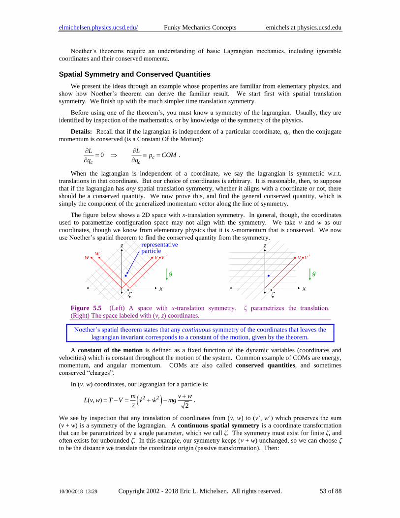
elmichelsen.physics.ucsd.edu/ Funky Mechanics Concepts emichels at physics.ucsd.edu
10/30/2018 13:29 Copyright 2002 - 2018 Eric L. Michelsen. All rights reserved. 53 of 88
Noether’s theorems require an understanding of basic Lagrangian mechanics, including ignorable
coordinates and their conserved momenta.
Spatial Symmetry and Conserved Quantities
We present the ideas through an example whose properties are familiar from elementary physics, and
show how Noether’s theorem can derive the familiar result. We start first with spatial translation
symmetry. We finish up with the much simpler time translation symmetry.
Before using one of the theorem’s, you must know a symmetry of the lagrangian. Usually, they are
identified by inspection of the mathematics, or by knowledge of the symmetry of the physics.
Details: Recall that if the lagrangian is independent of a particular coordinate, qc, then the conjugate
momentum is conserved (is a Constant Of the Motion):
0 cc c
L Lp COM
q q
= =
.
When the lagrangian is independent of a coordinate, we say the lagrangian is symmetric w.r.t.
translations in that coordinate. But our choice of coordinates is arbitrary. It is reasonable, then, to suppose
that if the lagrangian has any spatial translation symmetry, whether it aligns with a coordinate or not, there
should be a conserved quantity. We now prove this, and find the general conserved quantity, which is
simply the component of the generalized momentum vector along the line of symmetry.
The figure below shows a 2D space with x-translation symmetry. In general, though, the coordinates
used to parametrize configuration space may not align with the symmetry. We take v and w as our
coordinates, though we know from elementary physics that it is x-momentum that is conserved. We now
use Noether’s spatial theorem to find the conserved quantity from the symmetry.
x
w
z
v
g
v’w’
ζx
z
v
g
v’
ζ
representative particle
Figure 5.5 (Left) A space with x-translation symmetry. ζ parametrizes the translation.
(Right) The space labeled with (v, z) coordinates.
Noether’s spatial theorem states that any continuous symmetry of the coordinates that leaves the
lagrangian invariant corresponds to a constant of the motion, given by the theorem.
A constant of the motion is defined as a fixed function of the dynamic variables (coordinates and
velocities) which is constant throughout the motion of the system. Common example of COMs are energy,
momentum, and angular momentum. COMs are also called conserved quantities, and sometimes
conserved “charges”.
In (v, w) coordinates, our lagrangian for a particle is:
( )2 2( , )2 2
m v wL v w T V v w mg
+= − = + − .
We see by inspection that any translation of coordinates from (v, w) to (v’, w’) which preserves the sum
(v + w) is a symmetry of the lagrangian. A continuous spatial symmetry is a coordinate transformation
that can be parametrized by a single parameter, which we call ζ. The symmetry must exist for finite ζ, and
often exists for unbounded ζ. In this example, our symmetry keeps (v + w) unchanged, so we can choose ζ
to be the distance we translate the coordinate origin (passive transformation). Then:
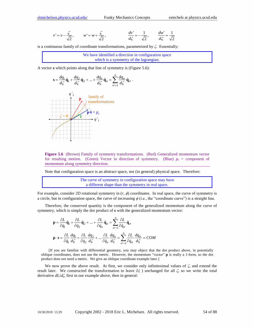
elmichelsen.physics.ucsd.edu/ Funky Mechanics Concepts emichels at physics.ucsd.edu
10/30/2018 13:29 Copyright 2002 - 2018 Eric L. Michelsen. All rights reserved. 54 of 88
' 1 ' 1' , ' , ,
2 2 2 2
dv dwv v w w
d d
= − = + = − =
is a continuous family of coordinate transformations, parametrized by ζ. Essentially:
We have identified a direction in configuration space
which is a symmetry of the lagrangian.
A vector s which points along that line of symmetry is (Figure 5.6):
1 21 2
1
ˆ ˆ ˆ ˆ...
nn
n
dq dqdq dq
d d d d
=
= + + + = s q q q q .
q’1ζ = 0
q’2family of
transformations
ŝ
p
p∙ŝ = ps
Figure 5.6 (Brown) Family of symmetry transformations. (Red) Generalized momentum vector
for resulting motion. (Green) Vector in direction of symmetry. (Blue) ps = component of
momentum along symmetry direction.
Note that configuration space is an abstract space, not (in general) physical space. Therefore:
The curve of symmetry in configuration space may have
a different shape than the symmetry in real space.
For example, consider 2D rotational symmetry in (r, ) coordinates. In real space, the curve of symmetry is
a circle, but in configuration space, the curve of increasing (i.e., the “coordinate curve”) is a straight line.
Therefore, the conserved quantity is the component of the generalized momentum along the curve of
symmetry, which is simply the dot product of s with the generalized momentum vector:
1 21 2 1
1 2
1 2 1
ˆ ˆ ˆ ˆ...
...
n
nn
nn
n
L L L L
q q q q
dq dqdq dqL L L LCOM
q d q d q d q d
=
=
= + + + =
= + + = =
p q q q q
p s
[If you are familiar with differential geometry, you may object that the dot product above, in potentially
oblique coordinates, does not use the metric. However, the momentum “vector” p is really a 1-form, so the dot
product does not need a metric. We give an oblique coordinate example later.]
We now prove the above result. At first, we consider only infinitesimal values of ζ, and extend the
result later. We constructed the transformation to leave L( ) unchanged for all ζ, so we write the total
derivative dL/dζ, first in our example above, then in general:
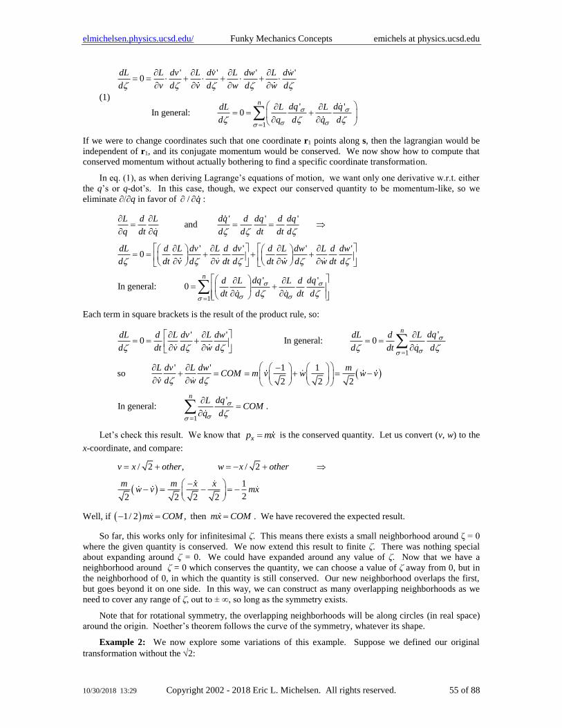
elmichelsen.physics.ucsd.edu/ Funky Mechanics Concepts emichels at physics.ucsd.edu
10/30/2018 13:29 Copyright 2002 - 2018 Eric L. Michelsen. All rights reserved. 55 of 88
(1)
1
' ' ' '0
' 'In general: 0
n
dL L dv L dv L dw L dw
d v d v d w d w d
dq dqdL L L
d q d q d
=
= = + + +
= = +
If we were to change coordinates such that one coordinate r1 points along s, then the lagrangian would be
independent of r1, and its conjugate momentum would be conserved. We now show how to compute that
conserved momentum without actually bothering to find a specific coordinate transformation.
In eq. (1), as when deriving Lagrange’s equations of motion, we want only one derivative w.r.t. either
the q’s or q-dot’s. In this case, though, we expect our conserved quantity to be momentum-like, so we
eliminate ∂/∂q in favor of / q :
1
' ' 'and
' ' ' '0
' 'In general: 0
n
L d L dq d dq d dq
q dt q d d dt dt d
dL d L dv L d dv d L dw L d dw
d dt v d v dt d dt w d w dt d
dq dqd L L d
dt q d q dt d
=
= = =
= = + + +
= +
Each term in square brackets is the result of the product rule, so:
( )
1
1
'' '0 In general: 0
' ' 1 1so
2 2 2
'In general: .
n
n
dqdL d L dv L dw dL d L
d dt v d w d d dt q d
L dv L dw mCOM m v w w v
v d w d
dqLCOM
q d
=
=
= = + = =
− + = = + = −
=
Let’s check this result. We know that xp mx= is the conserved quantity. Let us convert (v, w) to the
x-coordinate, and compare:
( )
/ 2 , / 2
1
22 2 2 2
v x other w x other
m m x xw v mx
= + = − +
− − = − = −
Well, if ( )1/ 2 , thenmx COM mx COM− = = . We have recovered the expected result.
So far, this works only for infinitesimal ζ. This means there exists a small neighborhood around ζ = 0
where the given quantity is conserved. We now extend this result to finite ζ. There was nothing special
about expanding around ζ = 0. We could have expanded around any value of ζ. Now that we have a
neighborhood around ζ = 0 which conserves the quantity, we can choose a value of ζ away from 0, but in
the neighborhood of 0, in which the quantity is still conserved. Our new neighborhood overlaps the first,
but goes beyond it on one side. In this way, we can construct as many overlapping neighborhoods as we
need to cover any range of ζ, out to ± ∞, so long as the symmetry exists.
Note that for rotational symmetry, the overlapping neighborhoods will be along circles (in real space)
around the origin. Noether’s theorem follows the curve of the symmetry, whatever its shape.
Example 2: We now explore some variations of this example. Suppose we defined our original
transformation without the 2:
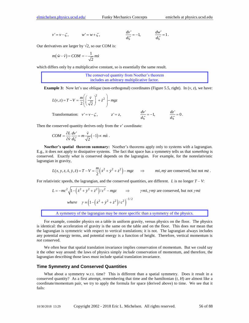
elmichelsen.physics.ucsd.edu/ Funky Mechanics Concepts emichels at physics.ucsd.edu
10/30/2018 13:29 Copyright 2002 - 2018 Eric L. Michelsen. All rights reserved. 56 of 88
' '' , ' , 1, 1
dv dwv v w w
d d
= − = + = − = .
Our derivatives are larger by 2, so our COM is:
( )1
2m w v COM mx− = = −
which differs only by a multiplicative constant, so is essentially the same result.
The conserved quantity from Noether’s theorem
includes an arbitrary multiplicative factor.
Example 3: Now let’s use oblique (non-orthogonal) coordinates (Figure 5.5, right). In (v, z), we have:
22( , )
2 2
' 'Transformation: ' , ' , 1, 0 .
m vL v z T V z mgz
dv dzv v z z
d d
= − = + −
= − = = − =
Then the conserved quantity derives only from the v’ coordinate:
( )'
12
L dv vCOM m mx
v d
= = −
.
Noether’s spatial theorem summary: Noether’s theorems apply only to systems with a lagrangian.
E.g., it does not apply to dissipative systems. The fact that space has a symmetry tells us that something is
conserved. Exactly what is conserved depends on the lagrangian. For example, for the nonrelativistic
lagrangian in gravity,
( )2 2 2( , , , , , ) , are conserved, but not2
mL x y z x y z T V x y z mgz mx my mz= − = + + − .
For relativistic speeds, the lagrangian, and the conserved quantities, are different. L is no longer T – V:
( )
( )( )
2 2 2 2 2
1/ 22 2 2 2
1 / , are conserved, but not
1 /
L mc x y z c mgz mx my mz
where x y z c
−
= − − + + −
− + +
A symmetry of the lagrangian may be more specific than a symmetry of the physics.
For example, consider physics on a table in uniform gravity, versus physics on the floor. The physics
is identical: the acceleration of gravity is the same on the table and on the floor. This does not mean that
the lagrangian is symmetric with respect to vertical translations; it is not. The lagrangian always includes
any potential energy terms, and potential energy is a function of height. Therefore, vertical momentum is
not conserved.
We often hear that spatial translation invariance implies conservation of momentum. But we could say
it the other way around: the laws of physics simply include conservation of momentum, and therefore, the
lagrangian describing those laws must include spatial translation invariance.
Time Symmetry and Conserved Quantities
What about a symmetry w.r.t. time? This is different than a spatial symmetry. Does it result in a
conserved quantity? As a first attempt, remembering that time and the hamiltonian (t, H) are almost like a
coordinate/momentum pair, we try to apply the formula for space (derived above) to time. We see that it
fails:
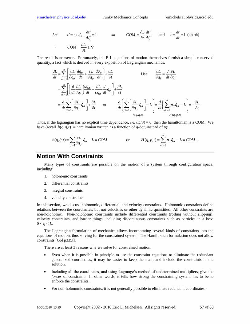
elmichelsen.physics.ucsd.edu/ Funky Mechanics Concepts emichels at physics.ucsd.edu
10/30/2018 13:29 Copyright 2002 - 2018 Eric L. Michelsen. All rights reserved. 57 of 88
' '' , 1 , and 1 (uh oh)
1??1
dt L dt dtLet t t COM t
d t d dt
LCOM
= + = = = =
=
The result is nonsense. Fortunately, the E-L equations of motion themselves furnish a simple conserved
quantity, a fact which is derived in every exposition of Lagrangian mechanics:
1
1
1 1
( , , )
Use:
n
i i
n
i
n n
h q q t
dq dqdL L L L L d L
dt q dt q dt t q dt q
dqd L L d Lq
dt q dt q dt t
d L L d Lq q L
dt q t dt q
=
=
= =
= + + =
= + +
= + −
1
( , , )
n
H q p t
d Lp q L
dt t
=
= − = −
Thus, if the lagrangian has no explicit time dependence, i.e. ∂L/∂t = 0, then the hamiltonian is a COM. We
have (recall ( , , )h q q t ≡ hamiltonian written as a function of q-dot, instead of p):
1 1
( , , ) or ( , , )
n nL
h q q t q L COM H q p t p q L COMq
= =
− = − =
.
Motion With Constraints
Many types of constraints are possible on the motion of a system through configuration space,
including:
1. holonomic constraints
2. differential constraints
3. integral constraints
4. velocity constraints
In this section, we discuss holonomic, differential, and velocity constraints. Holonomic constraints define
relations between the coordinates, but not velocities or other dynamic quantities. All other constraints are
non-holonomic. Non-holonomic constraints include differential constraints (rolling without slipping),
velocity constraints, and harder things, including discontinuous constraints such as particles in a box:
0 < q < L.
The Lagrangian formulation of mechanics allows incorporating several kinds of constraints into the
equations of motion, thus solving for the constrained system. The Hamiltonian formulation does not allow
constraints [Gol p335t].
There are at least 3 reasons why we solve for constrained motion:
• Even when it is possible in principle to use the constraint equations to eliminate the redundant
generalized coordinates, it may be easier to keep them all, and include the constraints in the
solution.
• Including all the coordinates, and using Lagrange’s method of undetermined multipliers, give the
forces of constraint. In other words, it tells how strong the constraining system has to be to
enforce the constraints.
• For non-holonomic constraints, it is not generally possible to eliminate redundant coordinates.
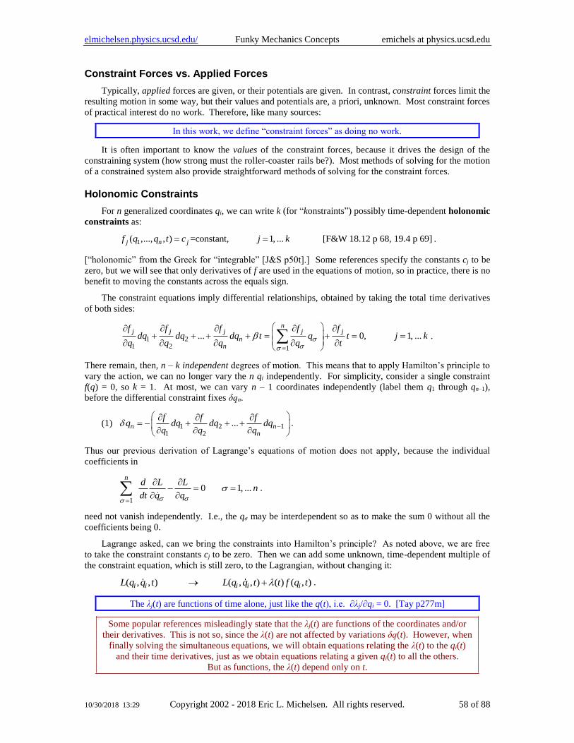
elmichelsen.physics.ucsd.edu/ Funky Mechanics Concepts emichels at physics.ucsd.edu
10/30/2018 13:29 Copyright 2002 - 2018 Eric L. Michelsen. All rights reserved. 58 of 88
Constraint Forces vs. Applied Forces
Typically, applied forces are given, or their potentials are given. In contrast, constraint forces limit the
resulting motion in some way, but their values and potentials are, a priori, unknown. Most constraint forces
of practical interest do no work. Therefore, like many sources:
In this work, we define “constraint forces” as doing no work.
It is often important to know the values of the constraint forces, because it drives the design of the
constraining system (how strong must the roller-coaster rails be?). Most methods of solving for the motion
of a constrained system also provide straightforward methods of solving for the constraint forces.
Holonomic Constraints
For n generalized coordinates qi, we can write k (for “konstraints”) possibly time-dependent holonomic
constraints as:
1( ,..., , ) =constant, 1, ... [F&W 18.12 p 68, 19.4 p 69]j n jf q q t c j k= = .
[“holonomic” from the Greek for “integrable” [J&S p50t].] Some references specify the constants cj to be
zero, but we will see that only derivatives of f are used in the equations of motion, so in practice, there is no
benefit to moving the constants across the equals sign.
The constraint equations imply differential relationships, obtained by taking the total time derivatives
of both sides:
1 21 2 1
... 0, 1, ...
nj j j j j
nn
f f f f fdq dq dq t q t j k
q q q q t
=
+ + + + = + = = .
There remain, then, n – k independent degrees of motion. This means that to apply Hamilton’s principle to
vary the action, we can no longer vary the n qi independently. For simplicity, consider a single constraint
f(q) = 0, so k = 1. At most, we can vary n – 1 coordinates independently (label them q1 through qn–1),
before the differential constraint fixes δqn.
(1) 1 2 11 2
...n nn
f f fq dq dq dq
q q q −
= − + + +
.
Thus our previous derivation of Lagrange’s equations of motion does not apply, because the individual
coefficients in
1
0 1, ...
nd L L
ndt q q
=
− = =
.
need not vanish independently. I.e., the qσ may be interdependent so as to make the sum 0 without all the
coefficients being 0.
Lagrange asked, can we bring the constraints into Hamilton’s principle? As noted above, we are free
to take the constraint constants cj to be zero. Then we can add some unknown, time-dependent multiple of
the constraint equation, which is still zero, to the Lagrangian, without changing it:
( , , ) ( , , ) ( ) ( , )i i i i iL q q t L q q t t f q t→ + .
The λj(t) are functions of time alone, just like the q(t), i.e. ∂λj/∂qi = 0. [Tay p277m]
Some popular references misleadingly state that the λj(t) are functions of the coordinates and/or
their derivatives. This is not so, since the λ(t) are not affected by variations δq(t). However, when
finally solving the simultaneous equations, we will obtain equations relating the λ(t) to the qi(t)
and their time derivatives, just as we obtain equations relating a given qi(t) to all the others.
But as functions, the λ(t) depend only on t.
elmichelsen.physics.ucsd.edu/ Funky Mechanics Concepts emichels at physics.ucsd.edu
10/30/2018 13:29 Copyright 2002 - 2018 Eric L. Michelsen. All rights reserved. 59 of 88
Therefore, when taking the variation of the trajectory, the δqi(t) do not affect the λj(t). Thus, for any
variation δqi(t) that satisfies the constraints:
(2)
1
( ) ( ) 0 [F&W 19.2 p69]
nB
A
L d L fS dt t q t
q dt q q
=
= − + =
.
As we freely vary the n – 1 independent coordinates, producing some unavoidable δqn(t), there must
exist, then, some λ(t), an as-yet undetermined function of time, which will cancel the forced variation of
δqn. [needs more explanation??] The λ(t) are called undetermined multipliers, since we don’t yet know
what they are. They are also called “Lagrange multipliers.”
[Many references state that “we can now vary all of the qi independently. I disagree. We can never
vary them independently because the constraint equation always applies, and prevents it.] We can now find
n equations of motion (not just n – 1 equations) by including the λ(t) to cancel the forced variations of the
dependent qn.
( ) 0, 1, ... (one constraint)L d L f
t nq dt q q
− + = =
.
We now have n equations of motion, 1 constraint equation, n unknown coordinate functions of time qi(t),
and 1 unknown undetermined multiplier λ(t). Thus we can solve the system of n + 1 differential equations
and n + 1 unknowns.
For k constraints (instead of just 1), note that we can freely vary n – k coordinates q1 through qn–k, and
we have k forced variations of qn–k+1 through qn. Then k undetermined multipliers λj(t) must exist which
together cancel the forced variations. This adds a summation over constraints to the equations of motion:
1
1
1
( , , ) ( ) ( , ) , ...
( ) 0 1, ... ( constraints)
k
i i j j i i n
j
kj
j
j
L L q q t t f q t where q q q
fL d Lt n k
q dt q q
=
=
= +
− + = =
Since constraints must include forces that guide the trajectory along constraint lines [F&W p52 ff], we
can include them in Lagrange’s Equations of Motion (LEM). Given n coordinates and k constraints, we
can rearrange the constraint equations to be additional equations of motion that give us a full system of
n + k equations for n + k dynamic variables. With the constraints defined as above,
(3) ,
1
( ) ( ) 1,..., [F&W 19.3 p69]
kj
j constraint
j
fd L Lt Q t n
dt q q q
=
− = =
,
which can be thought of as “rate of change of momentum − forces due to potentials = other forces.” The
other forces are exactly the n generalized forces of constraint Qσ(t),constraint, as functions of time.
These n equations plus the k constraint equations solve for the n qσ(t) and the k λj(t).
In the course of solving the equations, the qi(t) and λj(t) will have relations to the coordinates, including
their time derivatives possibly up to order 2(n – k), and possibly t. You solve for the qi(t) and λj(t)
simultaneously from the equations of motion, and the constraint equations. The solution can lead to
relations including such higher order derivatives of qi(t).
Generalized forces satisfy the same momentum and work equations as Cartesian forces:
,
(no sum on ), 1, ... [from F&W 15.4 p54]
( ) ( ), 1,..., [from (3) above]
i i
i i constraint ii i
W Q q i i n
d L Lp Q t Q t i n
dt q q
= =
= + =
elmichelsen.physics.ucsd.edu/ Funky Mechanics Concepts emichels at physics.ucsd.edu
10/30/2018 13:29 Copyright 2002 - 2018 Eric L. Michelsen. All rights reserved. 60 of 88
Differential Constraints
Differential constraints are written relating the differentials of coordinates, the coordinates, and
possibly time:
1 1 2 2
1
1
( , ) ( , ) ... ( , ) ( , ) ( , ) 0
1, ... , ... [F&W p71m]
n
j j jn n j j
n
q t dq q t dq q t dq dt q t dq q t dt
j k where q q q
=
+ + + + = + =
=
The jσ(qi, t) are functions of the coordinates and possibly time.
Recall that for holonomic constraints, in applying Hamilton’s principle (eq. (2)), we used only the
resulting differential constraint, Eq (1), where the ∂f/∂qi are also functions of the coordinates and time.
Therefore, differential constraints are also included in that part of the holonomic constraint analysis. With
a simple change of notation to the coefficients jσ, we have:
1
( , )( , ) : ( ) ( , ) ( ) 1, ...
[F&W p71b]
kj i
j i j j i
j
f q t d L Lq t t q t Q t n
q dt q q
=
→ − = =
However, we still need k constraint equations to augment the n equations of motion, to yield n + k
equations in all, needed to solve for n unknown qi(t) and k unknown λj(t). We get these by dividing the
differential constraint equation by dt. Physically, this means the instantaneous velocities of the coordinates
must obey the relationship:
1 1 2 2
1
( , ) ( , ) ... ( , ) ( , ) ( , ) 0
1, ... [F&W p71b]
n
j i j i jn i n j j i j iq t q q t q q t q q t q q t
j k
=
+ + + + = + =
=
[F&W p71b] note that this can be extended to the case where the j are functions of the velocities q-doti,
but give no references. Velocity constraints (described below) are tricky.
Constraints Including Velocities
The topic of velocity constraints has been fraught with much error and confusion, even among
physicists. We explain here several of the errors, and their corrections, citing published works along the
way.
Constraints including velocities are one kind of non-holonomic constraints. We can extend the
holonomic constraints by including the velocities in the constraint functions:
1 1( , ... , , ... , ) =constant 1, ...j n n jg q q q q t c j k= = .
Note that [Gol] has a serious error concerning velocity constraints.
[Thanks to Patrick Geisler for pointing this out to me.] The error is based on a 1966 paper [Ray1],
which was retracted the same year by the author [Ray2]. ([Gol p47b] also mistakenly cites the year as
1996.) Specifically, [Gol p47] (following [Ray1]) uses the method of Lagrangian multipliers with an
incorrect trajectory variation procedure, yielding an incorrect equation of motion. A corrected, but still
incomplete, procedure is given by [S&C1], [S&C2], and [J&S].
The error in [Ray1] and [Gol] derives from allowing variational trajectories which satisfy the
constraints, but which cannot be achieved by any physical constraining system. Specifically, for the
constraining mechanism to achieve the forces necessary for the trajectory, it would have to exert forces that
are not perpendicular to the motion, i.e. would have to violate D’Alembert’s Principle. In other words, the
constraining mechanism would have to “drag” the system in unphysical ways. Furthermore, even with
such a magical capability, the solution is not unique, because the equations are under-determined [J&S??].
elmichelsen.physics.ucsd.edu/ Funky Mechanics Concepts emichels at physics.ucsd.edu
10/30/2018 13:29 Copyright 2002 - 2018 Eric L. Michelsen. All rights reserved. 61 of 88
Clearly, any given physical system, with a full set of initial conditions, has only one (unique) motion
resulting from it.
[J&S p116t] claim that the correct variational procedure allows only trajectories which satisfy
d’Alembert’s principle (which is disputed by [Liu]). Surprisingly, such a variational procedure is very
simple. Instead of derivatives of the constraint equations with respect to the coordinates, we take
derivatives with respect to the velocities. We quote the result, which apparently even [J&S] are uneasy
about, since they only timidly endorse it, saying “this result is generally accepted....” [J&S p116t]:
,
1
( ) ( ) 1,..., [from J&S 3.21 p116t]
kj
j constraint
j
gd L Lt Q t n
dt q q q
=
− = =
.
It may seem that in taking the derivative of gj, we have lost information, but recall the that full constraint
equation is part of the set of equations used to finally solve the motion. Hence the information is retained.
However, the above equation is incomplete, because some of the k constraints may include only
coordinates (but not velocities), while others may include both [Liu (12) p752, and following]. How do we
simultaneously include both kinds of constraints? Furthermore, this result is based on d’Alembert’s
principle , which [Liu] claims is not valid for arbitrary velocity constraints, but only for a restricted class of
them.
Surprisingly, [Liu] addresses both of these problems in a 1981 paper that far predates [J&S]. Liu’s
approach uses F = ma directly, and therefore converts the original constraints into constraints on
acceleration. Liu’s prescription is:
2
2
( , )For each constraints of the form: ( , ) ( , , , )
( , , )For each constraints of the form: ( , , ) ( , , , )
jj j j
jj j j
f q tf q t c define h q q q t
t
g q q tg q q t c define h q q q t
t
=
=
By construction, the hj(·) (j = 1, ... k) form a set of k constraints, all of which are linear in the
accelerations. As before, the information lost in taking derivatives here is retained in the constraint
equations which form part of the complete set of simultaneous equations that must be solved for the
motion. Since [Liu] does not use Hamilton’s (or any other) variational principle, his most general
equations of motion are Newtonian and in 3D vector form. For N particles (and therefore 3N – k
independent degrees of freedom):
1
( ) , 1, ... [Liu (15) p752]k
ji i i j
ij
hm t i N
=
= + =
r F
r.
For those classes of constraints (described later) which satisfy d’Alembert’s principle, and therefore
also Hamilton’s principle, we can use generalized coordinates
,constraint
1
( ) ( ) [From Liu (19) p752]k
jj
j
hd L LQ t t
dt q q q
=
− = =
.
[Liu sec. 6 p753] derives d’Alembert’s principle, concluding:
d’Alembert’s principle is valid if and only if the constraints on the system are either (i) holonomic,
or (ii) homogeneous in velocity dependence.
By “homogeneous in velocity dependence” he means the velocity terms, taken separately from the
holonomic terms, are homogeneous (of any order) in the velocities. In other words, the constraint can be
written as:
( , , ) ( , ) ( , , ) ( , , ) is homogeneous in thei i i i i i i ig q q t f q t s q q t where s q q t q= + .
elmichelsen.physics.ucsd.edu/ Funky Mechanics Concepts emichels at physics.ucsd.edu
10/30/2018 13:29 Copyright 2002 - 2018 Eric L. Michelsen. All rights reserved. 62 of 88
Hamilton’s principle is valid only when d’Alembert’s principle is valid.
[Liu p752] points out that Newton’s 2nd law, F = ma, applies to all types of constraints, even when
Hamilton’s principle does not. Furthermore:
Newtonian-like equations of motion can be solved for the forces of constraint,
even when Hamilton’s principle does not apply.
Summary
We have shown that holonomic constraints can use the method of Lagrange undetermined multipliers
to solve simultaneously for all n of the interdependent qi(t), and for the undetermined multipliers λj(t). This
also provides the forces of constraint. Similarly, for differential constraints, the method of undetermined
multipliers solves for the motion and the forces of constraint, but uses a velocity relationship to supplement
Lagrange’s equations of motion.
Another variant of undetermined multipliers can be used to solve for integral constraints [Aro ch 8].
Velocity constraints have been widely misunderstood and incorrectly published by physicists for a
century. The most definitive work seems to be [Liu] in 1981, though his paper is only 4 pages. The final
result converts each constraint equation, whether a holonomic or velocity constraint, into an acceleration
constraint, which is necessarily linear in the accelerations. Undetermined multipliers once again provide
the final mathematical step to solve for the motion and constraint forces. d’Alembert’s principle, and
therefore Hamilton’s principle of stationary action, is only valid for holonomic constraints, and velocity
constraints whose velocity terms are homogeneous (of any order) in the velocities.
Newtonian-like equations of motion can be solved for the forces of constraint, even when Hamilton’s
principle does not apply.
elmichelsen.physics.ucsd.edu/ Funky Mechanics Concepts emichels at physics.ucsd.edu
10/30/2018 13:29 Copyright 2002 - 2018 Eric L. Michelsen. All rights reserved. 63 of 88
6 Hamiltonian Mechanics
Hamiltonian mechanics rewrites lagrangian mechanics in a different form, which is useful for many
applications. In particular, quantum mechanics starts with the Hamiltonian form of classical mechanics.
What Is the Hamiltonian?
The hamiltonian is defined as:
# coordinates
1
( , , ) ( , , ), [F&W 20.12 p79b]i i i i i i iii
LH q p t p q L q q t where p
q=
−
, (6.1)
where L is any lagrangian appropriate for the physics. Note that the hamiltonian is a function of
coordinates and momenta, whereas the lagrangian is a function of coordinates and their velocities.
Therefore, when transforming from the lagrangian to the hamiltonian, one must eliminate the velocities in
favor of the momenta using the definition of conjugate momentum, included in (6.1).
The units of the hamiltonian are always energy.
The units of a coordinate times its conjugate momentum are always action (energy-time).
This follows from the lagrangian having units of energy, and the definition of momentum in (6.1).
In the case of time invariant potentials, and nonrelativistic L = T – V, the above definition of H often
reduces to H = T + V. [Since some references address only this latter case in earlier discussions, they
confusingly define their hamiltonian in a highly nonstandard way [P&R 4.6 p43], though they fix it later in
the book.]
The hamiltonian is not defined as T + V.
Definition (6.1) allows for constrained velocities and time-dependent potentials.
[TBS: Bead on rotating hoop example. Linear bead on an accelerating (oscillating?) spring example.]
Note that constrained velocities usually require that the constraints do work on the system, thus changing
its energy over time.
Note that the value of the lagrangian function is always independent of the chosen generalized
coordinates, since it is defined by energy terms which are coordinate independent. In contrast [Gol p63t],
The values of the hamiltonian function depend on the coordinates chosen.
This can be seen from the defining equation above, which explicitly includes the coordinates and momenta,
along with the coordinate independent lagrangian. Later on, we’ll see that in electromagnetics, both the
lagrangian and hamiltonian are gauge-dependent.
It is not clear that the hamiltonian is well-defined for a dissipative system [ref??]. Hamiltonian
mechanics is generally used only for non-dissipative systems (which includes microscopic systems, such as
most elementary quantum systems).
The energy function: We can write the hamiltonian as a function of the qi and their velocities [Gol
??]:
1 1
( , , ) ( , , ) ( , , )n n
i i i i i i i i iii i
Lh q q t p q L q q t q L q q t
q= =
− = −
.
However, this is only the energy of the system in some cases, which we detail later.
TBS: How to hide time dependence in a system. For example, to add time-dependence to a given
mechanical system, we could define a new generalized coordinate, call it qt, with a constrained velocity and
initial condition:
elmichelsen.physics.ucsd.edu/ Funky Mechanics Concepts emichels at physics.ucsd.edu
10/30/2018 13:29 Copyright 2002 - 2018 Eric L. Michelsen. All rights reserved. 64 of 88
1, (0) 0 ( )t t tq q q t t= = = .
and then claim the hamiltonian is time-independent. The changes in energy that result are now due to the
“force” which is enforcing the constrained velocity on qt.
If the Hamiltonian Isn’t the Total Energy, Then What Is It?
If the hamiltonian is not the total energy, then what is its essential property? Much like the lagrangian,
we can define the hamiltonian in operational terms, i.e. what can I use it for? The hamiltonian of a system
is that function of the coordinates and their momenta for which Hamilton’s equations yield the correct
equations of motion. Equivalently, and importantly:
The essential property of the hamiltonian is that
it is the generator of time evolution for the system.
Given the state of a system at some time, and its hamiltonian, we can predict its future state for all time.
This property of generating time evolution is crucially important in classical mechanics, as well as quantum
mechanics.
For most quantum systems, the total energy function is the hamiltonian, but this is not the case for
relativistic fermions. Fermions satisfy the Dirac equation, and its hamiltonian is not the total energy. Too
many QM references insist on calling the hamiltonian the “energy,” which it clearly is not, when it is
perfectly simple and consistent to interpret it as the generator of time evolution.
When Does the Hamiltonian Equal Energy, and Other Questions?
There are three distinct questions we might ask about the hamiltonian:
1. Is the hamiltonian “conserved,” i.e. a constant of the motion?
2. Does the hamiltonian equal the total energy?
3. Does the hamiltonian equal T + V?
Note that [Gol p345]??
H may be the total energy, or not. H may be conserved, or not.
These are independent properties. A given H may be either, both, or neither.
It is not clear (to me, at least) that the hamiltonian is well-defined for a dissipative system, or that the
lagrangian is, either.
1. Is the hamiltonian conserved? This is simple: if the lagrangian does not explicitly depend on
time, then the hamiltonian is conserved:
( , , ) ( , )0 ( , ), 0, and 0, i.e., is conserved
L q q t H dH q pL L q q H
t t dt
= = = =
.
This follows directly from the equations of motion [F&W p80t]. Note that the modified equations of
motion which include friction (or drag) do not conserve the hamiltonian. Note that explicit time
dependence in the lagrangian is equivalent to explicit time dependence in the hamiltonian. Also, time-
dependent potentials lead to time-dependent lagrangians (and hamiltonians), and non-conservation of H.
2. Does the hamiltonian equal the energy? Sometimes the hamiltonian is the total energy;
sometimes it’s not. How to tell the difference? There are at least 4 equivalent ways to insure that H = total
energy, but as we show next, they are not necessary:
• When H = total energy, i.e., when you work out total energy as a function of the dynamic
variables (q, q-dot) or (q, p), and see that it equals H(q, p). This may seem trivial, but it works.
• When the generalized coordinates include all motion of the system, and all the forces derive from
a potential that is velocity independent [Gol p345]. This will lead to the preceding case.
elmichelsen.physics.ucsd.edu/ Funky Mechanics Concepts emichels at physics.ucsd.edu
10/30/2018 13:29 Copyright 2002 - 2018 Eric L. Michelsen. All rights reserved. 65 of 88
• When T (kinetic energy) is quadratic in the generalized velocities, i.e. is a homogeneous function
of degree 2 of the velocities [Arovas], and all the forces derive from a potential that is velocity
independent [Gol p345]. This homogeneity implies that all the motion of the system is included
by the generalized coordinates, which is the preceding case above. Note that the coefficients of
the quadratic velocity terms may be functions of the coordinates (i.e., need not be constant).
• When transformation of generalized coordinates to Cartesian coordinates does not explicitly
include the time, and all the forces derive from a potential that is velocity independent [Gol p345].
Note that total energy may be different than T + V if V = V(q, q-dot) includes velocities (see below). In
some cases, even though the lagrangian includes terms linear in velocities, the hamiltonian is still the total
energy. This happens with magnetic forces (more later).
Only conservative systems (no friction or drag) allow the hamiltonian to be the total energy.
Time independent constraints are insufficient to insure the hamiltonian be the total energy.
3. Does H = T + V? This depends on the conventions used by an author. If V = V(q) is the potential
energy as a function only of position, and there are no other forces, then H = T + V.
For velocity-dependent forces, such as the magnetic Lorentz force or Coriolis force in a rotating frame,
it is common to explicitly add another term to the lagrangian. For example, for a charged particle subject to
potential-forces and magnetic forces, we have (SI units):
1( , ) ( ) ( ) ( ,... ),
magnetic vector potential, electric charge
( ) position dependent potential
i i i i n
i
L q q T V q e q where q q
e
V q
= − +
q A q
A
Then numerically, H = T + V, which is the total energy, but its functional form includes A and the
canonical momentum pcan, so H is still the generator of time evolution (see below).
However, some references include velocity dependent potentials, such as the magnetic vector potential,
in V, which then becomes a function of positions and velocities [Aro 7.69]:
( )( , ) ( ) velocity-dependent forces
( , ) ( ) ( , ) (combined position-velocity potential)
V q q U q e
L q q T q V q q
−
= −
q A
In this case, V is a “potential,” but it is no longer a “potential energy,” since it includes a term which is not
an energy. This is just a change in notation that has no effect on the physics. Therefore, H ≠ T + V(q,
q-dot), but (as shown below) it does equal the total energy.
All Charged Up: The Magnetic Hamiltonian
It is interesting to compare the hamiltonian of a charged particle in a magnetic field to the total energy.
Many references say the hamiltonian is only the total energy if the “potential” is independent of velocity.
This statement is ambiguous, since it is not clear if the magnetic term in the lagrangian is considered a
“potential.” Regardless, the magnetic lagrangian term is linear in the particle velocity.
We compute the hamiltonian of a particle of charge e in a magnetic field, in 3D space, starting with the
lagrangian (in SI units):
elmichelsen.physics.ucsd.edu/ Funky Mechanics Concepts emichels at physics.ucsd.edu
10/30/2018 13:29 Copyright 2002 - 2018 Eric L. Michelsen. All rights reserved. 66 of 88
( )
2
2
2
( , ) ( ),2
( , ) ( )2
( )2
( ) ( ) total e2 2
can
m L eL e V m e
m
e m e eH L e V
m m m
e m ee V
m m
ee eV V
m m
−= + − = = + =
− − − − = − − +
− − = − − +
−− − = + = + =
p Ax x x x A x p p x A x
x
p A p A p Ax p p x p A x
p A p Ap A x
p Ap A p Ax x nergy
This reflects the fact that “kinetic momentum” pkin = mv = p – eA, and kinetic energy is (pkin)2/2m.
However:
Even though the magnetic lagrangian includes a velocity dependent term outside the kinetic
energy, the hamiltonian is indeed the total energy.
This example also illustrates that the hamiltonian is a function of the canonical momentum, and not the
kinetic momentum. The functional form of the hamiltonian is essential. For example, this magnetic force
hamiltonian satisfies:
( )2 2
hamiltonian hamiltonian
( , ) ( ) ( ) ( )2 2
kin
not
eH V T V V
m m
−= + = + = +
p A px p x x x .
The first equality gives the hamiltonian is its essential form, and defines the dynamics of the system; the
last equality is true numerically, but cannot be used to compute the dynamics of the system. In particular,
the last expression includes no information about the magnetic field.
Canonical Coordinates
Briefly, a canonical coordinate is a continuous real value that describes the position or orientation of
some part of the mechanical system. The conjugate momentum is the partial derivative of the lagrangian
with respect to the coordinate velocity:
( , , ),( , , ),1,...# degrees of motioni iL q q tL q q t
p or pq q
=
.
A canonical pair is the matched pair of a canonical coordinate with its conjugate momentum (qσ, pσ).
Example of a non-canonical coordinate: angle mod 2. It fully defines the physical configuration
(position) of the system, but cannot be used to analyze its dynamics, because it jumps discontinuously from
2π to 0 when wrapping around to the starting point. To be a valid coordinate, it must continue on with
values > 2π, so that its derivative is physically meaningful.
Are Coordinates Independent?
The following considerations are important to understanding Poisson brackets, as well as general
Lagrangian and Hamiltonian mechanics. They extend the above section “What Is the Derivative With
Respect To a Derivative?”
In Hamiltonian mechanics, we say things like 0a
b
p
q
=
, because pa and qb are “independent.” What
does this mean? Given a system, we can (in principle) solve it to find pa(t) and qb(t). Then in some
infinitesimal time interval dt, pa will change by an amount ( )a adp p t dt= , and qb will change by an amount
( )b bdq q t dt= . So you might be mislead into thinking that we could define the derivative dpa / dqb as the
ratio:
elmichelsen.physics.ucsd.edu/ Funky Mechanics Concepts emichels at physics.ucsd.edu
10/30/2018 13:29 Copyright 2002 - 2018 Eric L. Michelsen. All rights reserved. 67 of 88
( ) ( )0 (incorrect)
( ) ( )
a a a
b b b
dp p t dt p t
dq q t dt q t= = .
But in this case, the “derivative” a
b
dp
dq is ill-defined. pa(t) is not a function of qb, so how can it have any
derivative with respect to qb? Clearly, when we say that pa and qb are “independent,” we do not mean that
in the actual motion, one can change without the other changing.
So what does 0a
b
p
q
=
mean? Let us approach this through some simple examples. Consider a function:
2 3 2( , ) . Then 2 and 3X X
X c d c d c dc d
= + = =
.
We can avoid introducing the spurious function X by saying more directly,
( ) ( )2 3 2 3 22 and 3c d c c d dc d
+ = + =
.
On the other hand, X is a function, and we could describe this same function with different variables as
its arguments:
2 3 2( , ) . Then 2 and 3X X
X e f e f e fe f
= + = =
.
This new description has not changed the function X; we’ve simply changed the names of its arguments.
And we could still eliminate X entirely by writing:
( ) ( )2 3 2 3 22 3e f e and e f fe f
+ = + =
.
Returning to ∂pa/∂qb, let us change argument names again, and define:
2 3 2( , ) . Then 2 and 3b a b a b ab a
X XX q p q p q p
q p
= + = =
.
Or: ( ) ( )2 3 2 3 22 and 3b a b b a ab a
q p q q p pq p
+ = + =
.
Now consider a simpler function X:
( , ) . Then 0 and 1b a ab a
X XX q p p
q p
= = =
.
Or: ( ) 0 and 1a aa a
b b a a
p pp p
q q p p
= = = =
.
The first equation in the last line is the desired result. It means that, when “pa” is viewed as a function of
the dynamic variables, rather than as pa(t) [a function of time], then 0a
b
p
q
=
.
Similarly, the 2nd equation of the last line says that, when “pa” is viewed as a function of the dynamic
variables, rather than as pa(t) [a function of time], then 1a
a
p
p
=
.
elmichelsen.physics.ucsd.edu/ Funky Mechanics Concepts emichels at physics.ucsd.edu
10/30/2018 13:29 Copyright 2002 - 2018 Eric L. Michelsen. All rights reserved. 68 of 88
Lagrangian and Hamiltonian Relations #
1
, , , ,
[F&W 32.9, 32.11 p 175; 32.15a,b p 176; 32.29, 32.30 p 178]
coordinatesL H HL T V p H p q L p q
q q p
=
− − = − =
The hamiltonian depends on time only if it is explicitly time dependent:
[F&W 32.18 p 177]dH H L
dt t t
= = −
A conservative system implies a potential V(q) a function of coordinates only (but not time), and
holonomic time-independent constraints:
( , ) ( , ) ( )
(conservative holonomic, time-independent potential & constraints) [F&W 32.20 p 177]
H T V Energy const= + = =
q p q p q
Transformations
Point transformations involve only the coordinates and time (not velocities or momenta):
( )1, ..., , [F&W 32.4a p 174]nq q Q Q t = .
Canonical transformations involve coordinates and momenta for every transformed variable:
( )
( )
1 1
1 1
, ..., , , ..., , [F&W 34.1a,b p181]
, ..., , , ..., ,
n n
n n
p p P P Q Q t
q q P P Q Q t
=
=
For example, the central force transformation from 2-body problem to the 1-body problem is a
canonical transformation. In this case, the new canonical equations of motion separate into independent
equations for the center of mass motion and the orbiting motion. That’s why it’s so useful. Usually we can
ignore the center-of-mass motion, and focus only on the (now simpler) orbiting motion.
Canonical transformations preserve Hamilton’s Equations of Motion (HEM), phase-space volume, and
Poisson brackets. This means a transformation is canonical if and only if it has unit Jacobian (P&R 6.54 p
94):
( , )1
( , )
Q Q
q pQ P Q P P Q
P Pq p q p q p
q p
= = − =
.
Generating functions are functions of one old variable and one new variable. Time-independent
generating functions are F1(Q, q), F2(P, q), F3(Q, p), F4(P, p). [P&R Table 6.1 p 90]:
, , , , ( , ) ( , ) ( , )F F F F
q p Q P K Q P H Q P H q pp q P Q
= − = = = − = =
.
Time-dependent generating functions are F1(Q, q, t), F2(P, q, t), F3(Q, p, t), F4(P, p, t) [P&R , 6.60 p 95,
6.70 p 97]. (For comparison, F&W’s S(q, P, t) is like P&R’s F2(P, q) [F&W35.4a, b p184]):
( )
31 2 4
2
, ( , , ) ( , , ) ( , , )
( , , ) , ,
jFFF F FK Q P t H Q P t H q p t
t t t t t
S q P t F P q t
= = = = = +
.
How does the new lagrangian relate to the old lagrangian??
elmichelsen.physics.ucsd.edu/ Funky Mechanics Concepts emichels at physics.ucsd.edu
10/30/2018 13:29 Copyright 2002 - 2018 Eric L. Michelsen. All rights reserved. 69 of 88
1
2
3
4
( , ) ( , ) ( , , ) ( , , ) ( , )
( , , )
( , , )
( , , )
( , , )
dFH q p K Q P L q q t pq H L Q Q t PQ K Q P
dt
where F F q Q t
F F q P t Qp
F F p Q t qp
F F p P t qp QP
→ = − = = − +
=
= −
= −
= + −
For example, for F1(q, Q, t):
1
, ,
dF F F Fpq H PQ K PQ K q Q
dt t q Q
F F Fp P K H
q Q t
− = − + = − + + +
= − = − = +
Interesting and Useful Canonical Transforms
[From PD 26c]
a) Identity: 2( , ) ,F q P qP p P Q q= = = .
b) Interchange: 1( , ) ,F q Q qQ p Q P q= = = − .
Graphically demonstrates the interchangeability of ‘p’ and ‘q’ labels in Hamiltonian mechanics.
c) Point transform: 2( , ) ( ) , ( )df
F q P f q P p P Q f qdq
= = = .
d) Orthogonal transform: 2
,
( , ) ,i ik k i ki k k ik
i k k k
F q P Pa q p a P Q q a= = = .
Hamilton-Jacobi Theory
The goal is to transform so all the Q’s and P’s are constant, achieved by transforming H to zero.
F&W’s S(q, P, t) is like P&R’s F2(P, q) [F&W35.4a, b p 184, 35.12 p 185]:
1
1
, , ( , , ) ( , , ) 0
,..., , ,..., , 0n
n
S S Sp Q K H P Q t H p q t
q P t
S S SH q q t
q q t
S SP const and Q const
P
= = = = + =
+ =
= = = = = =
where all the P’s and Q’s are constant, and we rewrite them as α and β [F&W 35.15, 19, 20 p 186].
S(t) evaluated along the actual trajectory of the system is the action [F&W 35.23 p 187]:
dSL
dt= .
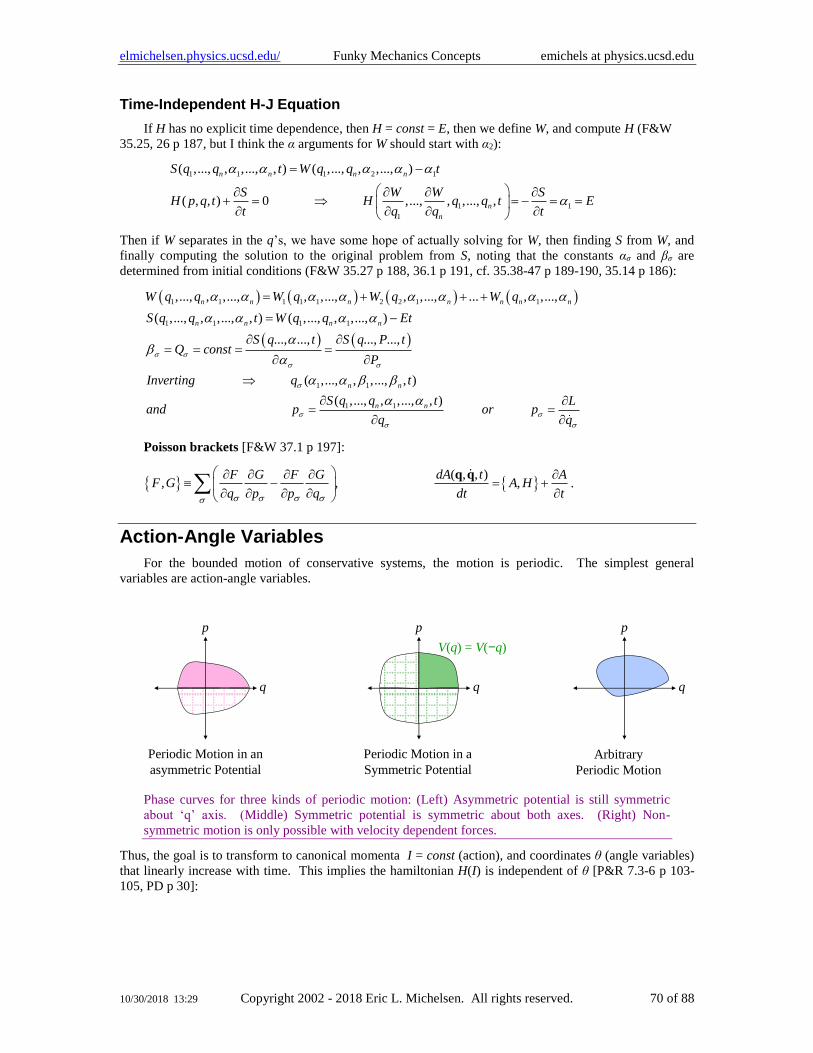
elmichelsen.physics.ucsd.edu/ Funky Mechanics Concepts emichels at physics.ucsd.edu
10/30/2018 13:29 Copyright 2002 - 2018 Eric L. Michelsen. All rights reserved. 70 of 88
Time-Independent H-J Equation
If H has no explicit time dependence, then H = const = E, then we define W, and compute H (F&W
35.25, 26 p 187, but I think the α arguments for W should start with α2):
1 1 1 2 1
1 1
1
( ,..., , ,..., , ) ( ,..., , ,..., )
( , , ) 0 ,..., , ,..., ,
n n n n
n
n
S q q t W q q t
S W W SH p q t H q q t E
t q q t
= −
+ = = − = =
Then if W separates in the q’s, we have some hope of actually solving for W, then finding S from W, and
finally computing the solution to the original problem from S, noting that the constants ασ and βσ are
determined from initial conditions (F&W 35.27 p 188, 36.1 p 191, cf. 35.38-47 p 189-190, 35.14 p 186):
( ) ( ) ( ) ( )
( ) ( )
1 1 1 1 1 2 2 1 1
1 1 1 1
1 1
,..., , ,..., , ,..., , ,..., ... , ,...,
( ,..., , ,..., , ) ( ,..., , ,..., )
..., ..., ..., ...,
( ,..., , ,..., , )
n n n n n n n
n n n n
n n
W q q W q W q W q
S q q t W q q Et
S q t S q P tQ const
P
Inverting q t
a
= + + +
= −
= = = =
1 1( ,..., , ,..., , )n nS q q t Lnd p or p
q q
= =
Poisson brackets [F&W 37.1 p 197]:
( , , )
, , ,F G F G dA t A
F G A Hq p p q dt t
− = +
q q.
Action-Angle Variables
For the bounded motion of conservative systems, the motion is periodic. The simplest general
variables are action-angle variables.
Arbitrary
Periodic Motion
Periodic Motion in an
asymmetric Potential
Periodic Motion in a
Symmetric Potential
V(q) = V(−q)
p
q
p
q
p
q
Phase curves for three kinds of periodic motion: (Left) Asymmetric potential is still symmetric
about ‘q’ axis. (Middle) Symmetric potential is symmetric about both axes. (Right) Non-
symmetric motion is only possible with velocity dependent forces.
Thus, the goal is to transform to canonical momenta I = const (action), and coordinates θ (angle variables)
that linearly increase with time. This implies the hamiltonian H(I) is independent of θ [P&R 7.3-6 p 103-
105, PD p 30]:
elmichelsen.physics.ucsd.edu/ Funky Mechanics Concepts emichels at physics.ucsd.edu
10/30/2018 13:29 Copyright 2002 - 2018 Eric L. Michelsen. All rights reserved. 71 of 88
( )0 (constant of motion),
( ) ( )( ) ( ) ( )
H II I COM
H I E II COM t I t
I I
= − = =
= = = = = +
F&W say the “angles” are not canonical conjugates of the action [F&W 36.13 p193], but PD says
they’re wrong. The above eqs are Hamilton’s, and [P&R p106 and many others] and [PD p33] say “the
transformation (q, p) → (θ, I) is canonical”.
The action variable has dimensions of action = angular momentum = energy-time. The angle variable
is dimensionless (P&R p 107). For libration (oscillation), action can be computed from E and V [P&R
7.10-14 p106-107]:
( )
( )
( )
2
max
min
max
0
( , ) ( ) ( , ) 2 ( )2
phase-space-area 1 1( ) ( , ) [arbitrary phase curve]
2 2 2
12 ( ) [particle in simple potential]
22 ( ) [particle in symmetri
q
q
q
e
pH q p E V q p q E m E V q
m
I E dq dp dq p q E
dq m E V q
dq m E V q
−
−
−
= = + = −
= = =
= −
= −
c potential ( ) ( )]e eV q V q= −
The turning points qmin and qmax are where T = 0, or E = V, or velocity = 0.
Abbreviated action is the generating function for the action-angle canonical transform [P&R 7.29 p
112]:
2 20
( , ) ( , ) ( , )q
F q I S q I dq p q I= = .
For periodic motion (rotations), simply change the above integration limits to one period, and rename q = ψ
(P&R 7.44, 7.46 p114, cf. 7.51 p115). However, P&R assume a period of 2π in the original coordinate ψ
(not just the transformed coordinate θ), which is bad (e.g., P&R problem 7.2: original period is 4π):
( )( , ) ( 2 , ) ( , ) 2 ( )
1( ) ( , )
2 T
H q p H p p E m E V
I E d p E
= = + = −
=
Action-angle variables for the linear (i.e. harmonic) oscillator:
22 2
1/ 2
2 2
1( , , )
2
2 2sin , 2 sin 2 cos
pH q p t m q
m
I Iq p m I m m I
m
= +
= = − =
Small Oscillations: Summary and Example
Introduction: A persistent challenge in mechanical engineering is designing machines that preserve
their integrity, and are compatible with their surroundings. In other words, they don’t fall apart, and don’t
jump around too much when they operate. Such machines are designed to restrain unwanted motion, but
this can never be fully achieved. This very restraint necessarily leads to “small” oscillations. To control
them, one must first understand them. We describe here undamped small oscillations. Real machines
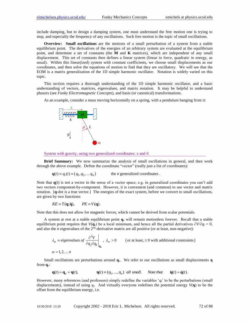
elmichelsen.physics.ucsd.edu/ Funky Mechanics Concepts emichels at physics.ucsd.edu
10/30/2018 13:29 Copyright 2002 - 2018 Eric L. Michelsen. All rights reserved. 72 of 88
include damping, but to design a damping system, one must understand the free motion one is trying to
stop, and especially the frequency of any oscillations. Such free motion is the topic of small oscillations.
Overview: Small oscillations are the motions of a small perturbation of a system from a stable
equilibrium point. The derivatives of the energies of an arbitrary system are evaluated at the equilibrium
point, and determine a set of constants (the M and K matrices), which are independent of any small
displacement. This set of constants then defines a linear system (linear in force, quadratic in energy, as
usual). Within this linear(ized) system with constant coefficients, we choose small displacements as our
coordinates, and then solve the equations of motion to find that they are oscillatory. We will see that the
EOM is a matrix generalization of the 1D simple harmonic oscillator. Notation is widely varied on this
topic.
This section requires a thorough understanding of the 1D simple harmonic oscillator, and a basic
understanding of vectors, matrices, eigenvalues, and matrix notation. It may be helpful to understand
phasors (see Funky Electromagnetic Concepts), and basis (or canonical) transformations.
As an example, consider a mass moving horizontally on a spring, with a pendulum hanging from it:
x
M
m
L
k
g
System with gravity, using two generalized coordinates: x and θ.
Brief Summary: We now summarize the analysis of small oscillations in general, and then work
through the above example. Define the coordinate “vector” (really just a list of coordinates):
( )1 2( ) ( ) , , ... the generalized coordinatesi nt q t q q q n q .
Note that q(t) is not a vector in the sense of a vector space; e.g. in generalized coordinates you can’t add
two vectors component-by-component. However, it is convenient (and common) to use vector and matrix
notation. [q-dot is a true vector.] The energies of the exact system, before we convert to small oscillations,
are given by two functions:
( ; ), ( )KE T PE V q q q .
Note that this does not allow for magnetic forces, which cannot be derived from scalar potentials.
A system at rest at a stable equilibrium point qe will remain motionless forever. Recall that a stable
equilibrium point requires that V(qe) be a local minimum, and hence all the partial derivatives ∂V/∂qi = 0,
and also the n eigenvalues of the 2nd-derivative matrix are all positive (or at least, non-negative):
( )2
, 0 or at least, 0 with additional constraints
1,2, ...
ej k
Veigenvalues of
q q
n
=
q
Small oscillations are perturbations around qe. We refer to our oscillations as small displacements η
from qe:
1( ) ( ), ( ) ( , ..., ) . ( ) ( )e nt t t all small Note that t t = + =q q η η η q .
However, many references (and professors) simply redefine the variables ‘qi’ to be the perturbations (small
displacements), instead of using ηj. And virtually everyone redefines the potential energy V(η) to be the
offset from the equilibrium energy, i.e.
elmichelsen.physics.ucsd.edu/ Funky Mechanics Concepts emichels at physics.ucsd.edu
10/30/2018 13:29 Copyright 2002 - 2018 Eric L. Michelsen. All rights reserved. 73 of 88
( ) ( ) ( ) ( ) ( )e e eV V V V V − = + −η q q q η q .
Then, in the perturbation coordinates, η:
, 1 , 1
1 1 1 1,
2 2 2 2
n nT T
jk j k jk j k
j k j k
KE T M PE V K = =
= = = = η Mη η Kη .
The kinetic energy is a quadratic form of the generalized velocities, and the potential energy is a
quadratic form of the generalized (small displacement) coordinates. (This again reveals the limitation of no
magnetic forces.) The above forms show that we can populate the M and K matrices from the 2nd
derivatives of the kinetic and potential energies:
(1) 2 2 2 2( ) ( ) ( ) ( )
,
e e
jk jkj k j k j k j k
T T V VM K
q q q q
= = = =
q q
η q q,
which contain only constant terms (i.e., no η).
The whole system of small oscillations is based on the displacements η(t) being small. Therefore, M
and K have only constant terms (the kinetic and potential energies are Taylor expanded to 2nd order), so the
energies are quadratic in the η. Higher order terms are neglected. This insures that:
The M and K matrices are constants (contain no η or derivatives).
They are also symmetric, and positive definite.
Finally, note that since the generalized coordinates have different units (x in m, θ in rad):
The matrix elements of M can have different units from each other,
as can the elements of K.
The equation of motion (EOM) can be found from Euler-Lagrange, and turns out to be:
which looks a lot like the ODE oscillator case: mx kx= − = −Mη Kη .
This is a linear differential equation with constant coefficients in the vector η. [If we have arrived at the
equation of motion somehow, we can populate the M and K matrices from it. That’s usually much more
work than taking derivatives of the T(η-dot) and V(η) functions.] We can solve it similarly to the ODE, by
converting to Fourier space (aka Fourier modes, or simply phasors). Analogously to the ODE case, we
expect the result to be sinusoidal oscillations in time. Then we use the complex-valued phasor vector a to
represent the sinusoids (a is not acceleration):
( ) ( )2
2
2
2
( ) Re is yet to be determined
, , and we have
, or
i tt e where
d di
dt dt
+=
→ → −
− = −
η a
Ma Ka
(2) ( )2− = vK M a 0 .
Note that a is a constant phasor vector, and the time dependence is exp(+iωt), not the usual physics
convention of “–iωt”.
[Aside: instead of a complex phasor, we could have simply assumed that the solution has the form:
( )
( )
( )
1 1
2 2
cos
cos( )
:
cosn n
A t
A tt
A t
+
+ =
+
η ,
elmichelsen.physics.ucsd.edu/ Funky Mechanics Concepts emichels at physics.ucsd.edu
10/30/2018 13:29 Copyright 2002 - 2018 Eric L. Michelsen. All rights reserved. 74 of 88
which yields the same transformation for the 2nd derivative, ∂2/dt2 → –ω2, but the later algebra is simpler in the
complex form.]
Now our equation for the complex vector a, eq. (2), can be viewed as a system of n linear equations in
n unknowns: the components aj. It has a non-trivial solution only if the determinant:
2 20 or equivalently 0 − = − =K M M K .
Since we will be solving for ω2, we avoid many minus signs by using the form on the right, above. This
determinant is an nth order polynomial in ω2, so it yields n discrete values of ω2, which will all be positive.
For each ω2, we choose the positive square root +ω, since the negative root simply duplicates the solution
of the positive root. Thus:
There are n discrete values of ω, all real, for each of which
a solution to the system of small displacements exists.
[F&W p??] say the ω can be degenerate. If so, then we can construct orthogonal eigenvectors in the
usual way, such as with Graham-Schmidt orthogonalization. The set of ω are the generalized eigenvalues
of the generalized eigenvector equation, eq. (2) above. [If M were the identity, it would be a standard
eigenvector equation.] We solve it by simply solving the set of simultaneous equations, with ordinary
algebra. Each frequency, ωα, yields a distinct phasor eigenvector, aα, which represents a solution to the
small oscillations:
( ) Re 1,2,...i t
t e n +
= =η a .
Thus we have n linearly independent solutions to the equations of motion, ηα(t), each of which is a
complete set of n coordinate functions of time. Recall that eigenvectors are only defined up to a
multiplicative constant.
Now the matrices M and K are symmetric (i.e., self-adjoint) and positive-definite, which implies the
eigenvectors aα can be chosen to be purely real. This means for a single frequency ωα (i.e., for a single
mode), all the coordinates ηi(t) cross their zero-points at the same time, i.e. they are all either in-phase or
exactly out-of-phase.
Also, eq. (2) is linear, so any multiple of a solution is also a solution, and any linear combination of
solutions is a solution. This means we have:
( )
( )1
( ) cos is real, and
( ) cos ( ) is the most general solution .n
t A t where
t A t where t
=
= +
= +
η a a
η a η
The 2n free parameters Aα and δα are the amplitudes and phases of the oscillations, and can be chosen to
satisfy 2n “boundary conditions” (really, any 2n constraints on the solution, be they at the boundary or not).
In such a combination of modes of oscillation, the coordinates ηi(t) no longer cross their zero-points
simultaneously.
The modes of oscillation act independently of each other.
Therefore, it is often useful to transform to a set of n coordinates where each coordinate represents a single
mode of oscillation. By simply rearranging the above general solution for η(t), we can define normal
coordinates ξα(t) such that:
( ) ( )1 1
( ) cos ( ) ( ) cosn n
t A t t where t A t
= =
= + + η a a .
(Such a transformation often comes up in quantum mechanics, because the resulting normal coordinates are
simple harmonic oscillators, and are quantized as such, in the usual quantum way.) Continuing classically,
though:
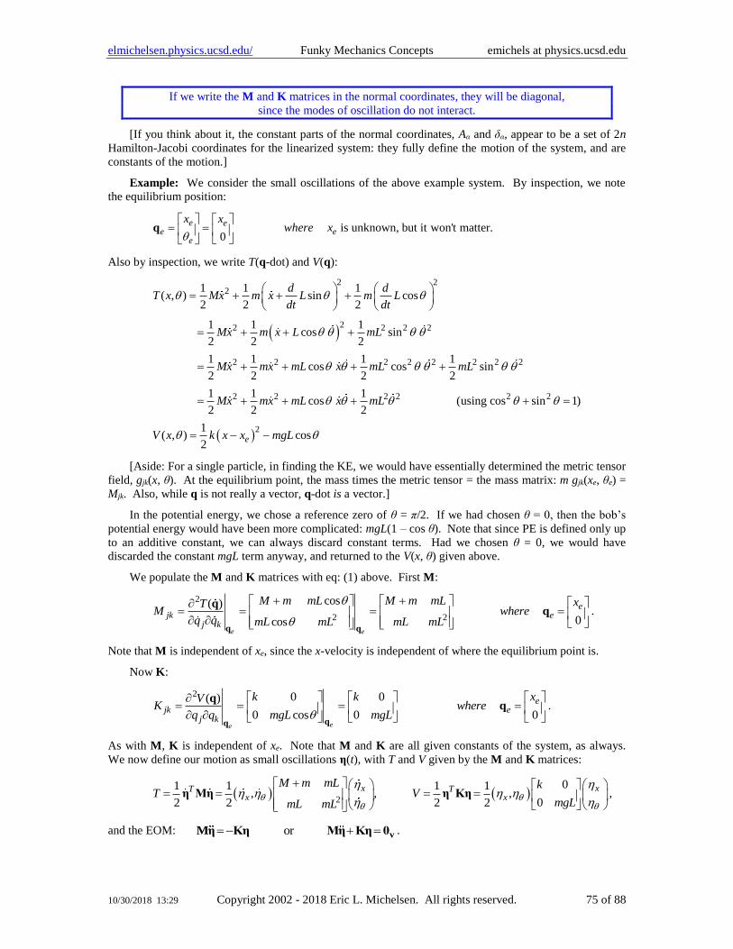
elmichelsen.physics.ucsd.edu/ Funky Mechanics Concepts emichels at physics.ucsd.edu
10/30/2018 13:29 Copyright 2002 - 2018 Eric L. Michelsen. All rights reserved. 75 of 88
If we write the M and K matrices in the normal coordinates, they will be diagonal,
since the modes of oscillation do not interact.
[If you think about it, the constant parts of the normal coordinates, Aα and δα, appear to be a set of 2n
Hamilton-Jacobi coordinates for the linearized system: they fully define the motion of the system, and are
constants of the motion.]
Example: We consider the small oscillations of the above example system. By inspection, we note
the equilibrium position:
is unknown, but it won't matter.0
e ee e
e
x xwhere x
= =
q
Also by inspection, we write T(q-dot) and V(q):
( )
2 22
22 2 2 2
2 2 2 2 2 2 2 2
2 2 2 2 2 2
1 1 1( , ) sin cos
2 2 2
1 1 1cos sin
2 2 2
1 1 1 1cos cos sin
2 2 2 2
1 1 1cos (using cos sin 1)
2 2 2
(
d dT x Mx m x L m L
dt dt
Mx m x L mL
Mx mx mL x mL mL
Mx mx mL x mL
V x
= + + +
= + + +
= + + + +
= + + + + =
( )21
, ) cos2
ek x x mgL = − −
[Aside: For a single particle, in finding the KE, we would have essentially determined the metric tensor
field, gjk(x, θ). At the equilibrium point, the mass times the metric tensor = the mass matrix: m gjk(xe, θe) =
Mjk. Also, while q is not really a vector, q-dot is a vector.]
In the potential energy, we chose a reference zero of θ = π/2. If we had chosen θ = 0, then the bob’s
potential energy would have been more complicated: mgL(1 – cos θ). Note that since PE is defined only up
to an additive constant, we can always discard constant terms. Had we chosen θ = 0, we would have
discarded the constant mgL term anyway, and returned to the V(x, θ) given above.
We populate the M and K matrices with eq: (1) above. First M:
2
2 2
cos( )
0cose e
ejk e
j k
M m mL M m mL xTM where
q q mL mL mL mL
+ + = = = =
q q
qq .
Note that M is independent of xe, since the x-velocity is independent of where the equilibrium point is.
Now K:
2 0 0( )
0 cos 0 0ee
ejk e
j k
k k xVK where
mgL mgLq q
= = = =
qq .
As with M, K is independent of xe. Note that M and K are all given constants of the system, as always.
We now define our motion as small oscillations η(t), with T and V given by the M and K matrices:
( ) ( )2
01 1 1 1, , ,
02 2 2 2
x xT Tx x
M m mL kT V
mgLmL mL
+ = = = =
η Mη η Kη ,
and the EOM: or= − + = vMη Kη Mη Kη 0 .
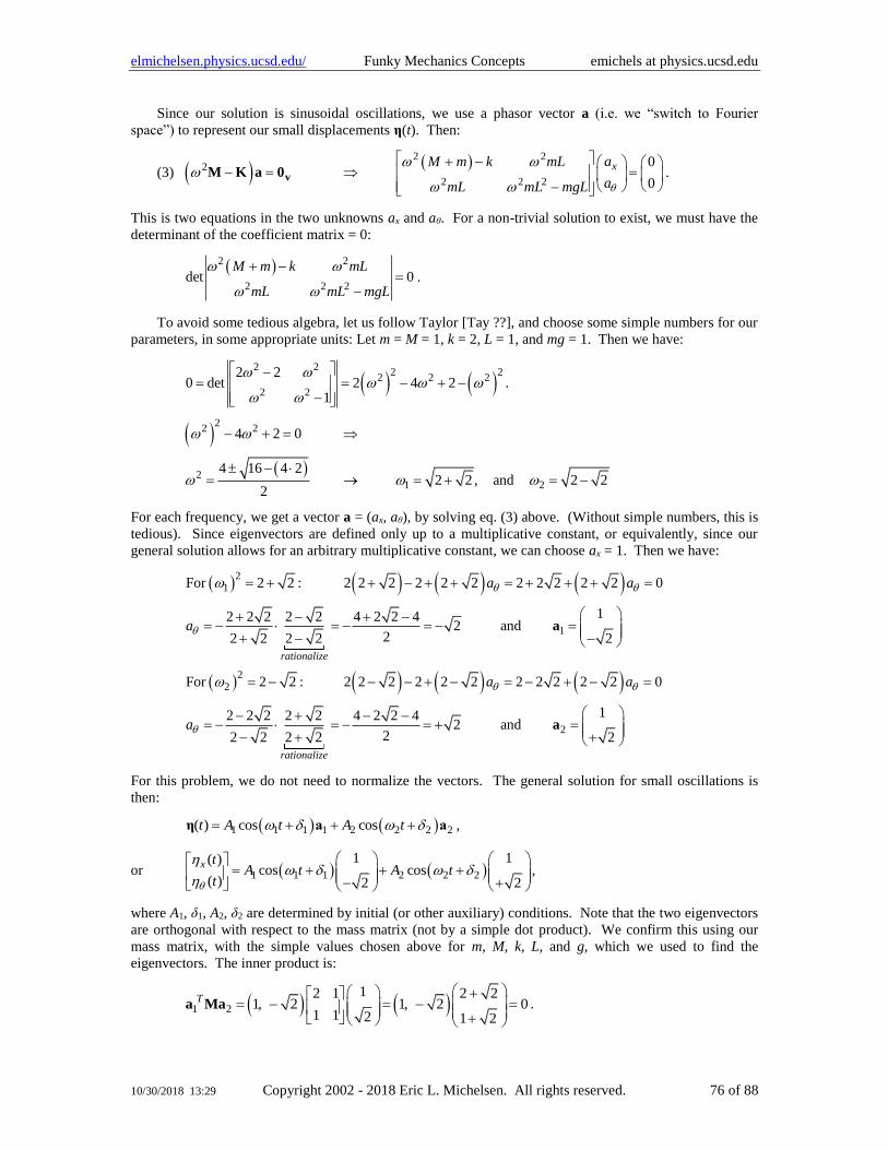
elmichelsen.physics.ucsd.edu/ Funky Mechanics Concepts emichels at physics.ucsd.edu
10/30/2018 13:29 Copyright 2002 - 2018 Eric L. Michelsen. All rights reserved. 76 of 88
Since our solution is sinusoidal oscillations, we use a phasor vector a (i.e. we “switch to Fourier
space”) to represent our small displacements η(t). Then:
(3) ( )( )2 2
2
2 2 2
0
0
xaM m k mL
amL mL mgL
+ − − = =
− vM K a 0 .
This is two equations in the two unknowns ax and aθ. For a non-trivial solution to exist, we must have the
determinant of the coefficient matrix = 0:
( )2 2
2 2 2det 0
M m k mL
mL mL mgL
+ −=
−.
To avoid some tedious algebra, let us follow Taylor [Tay ??], and choose some simple numbers for our
parameters, in some appropriate units: Let m = M = 1, k = 2, L = 1, and mg = 1. Then we have:
( ) ( )
( )
( )
2 22 2
2 2 2
2 2
22 2
21 2
2 20 det 2 4 2 .
1
4 2 0
4 16 4 22 2 , and 2 2
2
−= = − + −
−
− + =
− = → = + = −
For each frequency, we get a vector a = (ax, aθ), by solving eq. (3) above. (Without simple numbers, this is
tedious). Since eigenvectors are defined only up to a multiplicative constant, or equivalently, since our
general solution allows for an arbitrary multiplicative constant, we can choose ax = 1. Then we have:
( ) ( ) ( ) ( )
( ) ( ) ( ) ( )
21
1
22
2
For 2 2 : 2 2 2 2 2 2 2 2 2 2 2 0
12 2 2 2 2 4 2 2 42 and
22 2 2 2 2
For 2 2 : 2 2 2 2 2 2 2 2 2 2 2 0
12 2 2 2 2 4 2 2 42 and
22 2 2 2 2
rationalize
rationalize
a a
a
a a
a
= + + − + + = + + + =
+ − + −= − = − = − = + − −
= − − − + − = − + − =
− + − −= − = − = + = − + +
a
a
For this problem, we do not need to normalize the vectors. The general solution for small oscillations is
then:
( ) ( )1 1 1 1 2 2 2 2( ) cos cost A t A t = + + +η a a ,
or ( ) ( )1 1 1 2 2 2
1 1( )cos cos
( ) 2 2
x tA t A t
t
= + + + − +
,
where A1, δ1, A2, δ2 are determined by initial (or other auxiliary) conditions. Note that the two eigenvectors
are orthogonal with respect to the mass matrix (not by a simple dot product). We confirm this using our
mass matrix, with the simple values chosen above for m, M, k, L, and g, which we used to find the
eigenvectors. The inner product is:
( ) ( )1 2
12 1 2 21, 2 1, 2 0
1 1 2 1 2
T +
= − = − = +
a Ma .
elmichelsen.physics.ucsd.edu/ Funky Mechanics Concepts emichels at physics.ucsd.edu
10/30/2018 13:29 Copyright 2002 - 2018 Eric L. Michelsen. All rights reserved. 77 of 88
Summary
• Small oscillations are important real-world phenomena.
• They are analyzed as a matrix-vector generalization of the simple harmonic oscillator.
• A system has n natural frequencies, where n is the number of degrees of freedom (degrees of motion).
• Each frequency is a “mode” of oscillation, in which the generalized coordinates all oscillate
sinusoidally, with the relative amplitudes fixed; the phases can all be taken as 0, with some of the
amplitudes negative. In other words, all coordinates of a single mode go through zero simultaneously.
• The general solution is a linear superposition of all n modes, where the zero-crossings are, in general,
no longer simultaneous.
• The motion has 2n arbitrary constants, which can be used to match 2n initial (or other) conditions.
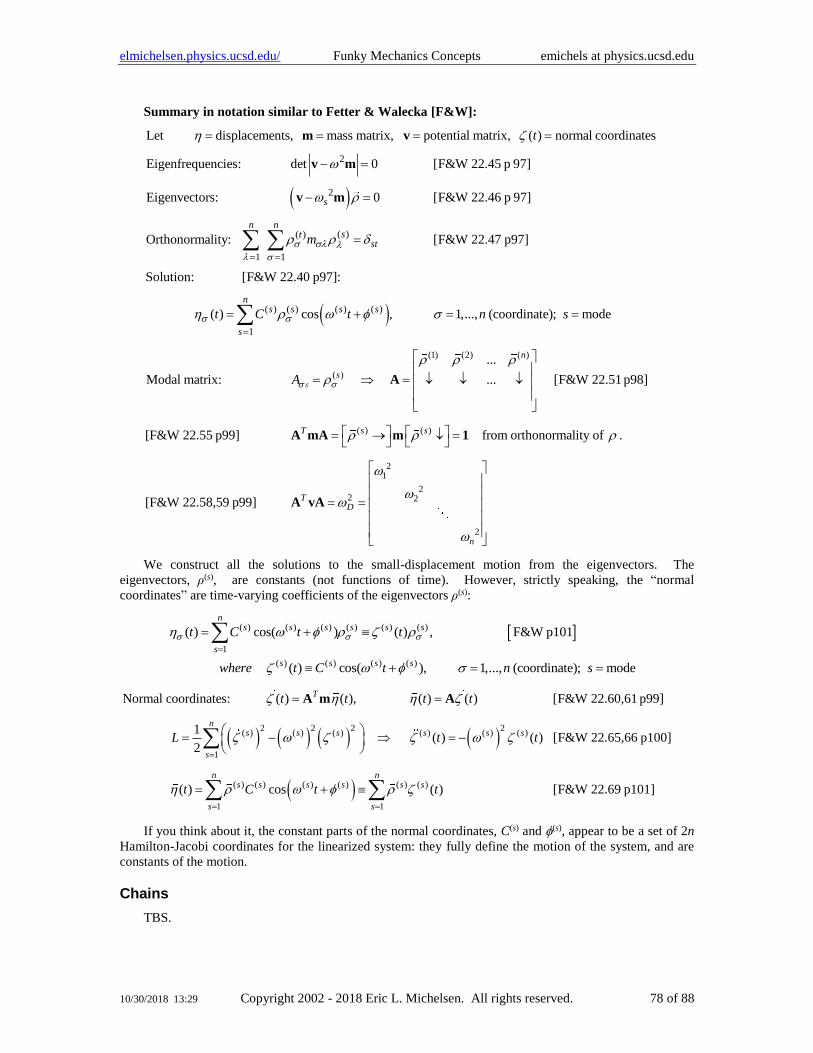
elmichelsen.physics.ucsd.edu/ Funky Mechanics Concepts emichels at physics.ucsd.edu
10/30/2018 13:29 Copyright 2002 - 2018 Eric L. Michelsen. All rights reserved. 78 of 88
Summary in notation similar to Fetter & Walecka [F&W]:
( )
2
2
( )( )
1 1
Let displacements, mass matrix, potential matrix, ( ) normal coordinates
Eigenfrequencies: det 0 [F&W 22.45 p 97]
Eigenvectors: 0 [F&W 22.46 p 97]
Orthonormality:
s
n nst
t
m
= =
= = = =
− =
− =
=
m v
v m
v m
( )( ) ( ) ( ) ( )
1
[F&W 22.47 p97]
Solution: [F&W 22.40 p97]:
( ) cos , 1,..., (coordinate); mode
st
ns s s s
s
t C t n s
=
= + = =
(1) (2) ( )
( )
( ) ( )
21
22 2
2
...
Modal matrix: ... [F&W 22.51 p98]
[F&W 22.55 p99] from orthonormality of .
[F&W 22.58,59 p99]
n
s
T s s
TD
n
A
= =
= → =
= =
A
A mA m 1
A vA
s
We construct all the solutions to the small-displacement motion from the eigenvectors. The
eigenvectors, ρ(s), are constants (not functions of time). However, strictly speaking, the “normal
coordinates” are time-varying coefficients of the eigenvectors ρ(s):
( ) ( ) ( ) ( ) ( ) ( )
1
( ) ( ) ( ) ( )
( ) cos( ) ( ) ,
( ) cos( ), 1,..., (coordinate); mode
F&W p101
ns s s s s s
s
s s s s
t C t t
where t C t n s
=
= +
+ = =
( ) ( ) ( ) ( )
( )
2 2 2 2( ) ( ) ( ) ( ) ( ) ( )
1
( ) ( ) ( ) ( ) ( ) ( )
1 1
Normal coordinates: ( ) ( ), ( ) ( ) [F&W 22.60,61 p99]
1( ) ( ) [F&W 22.65,66 p100]
2
( ) cos ( ) [F&W 22.69 p101]
T
ns s s s s s
s
n ns s s s s s
s s
t t t t
L t t
t C t t
=
= =
= =
= − = −
= +
A m A
If you think about it, the constant parts of the normal coordinates, C(s) and (s), appear to be a set of 2n
Hamilton-Jacobi coordinates for the linearized system: they fully define the motion of the system, and are
constants of the motion.
Chains
TBS.
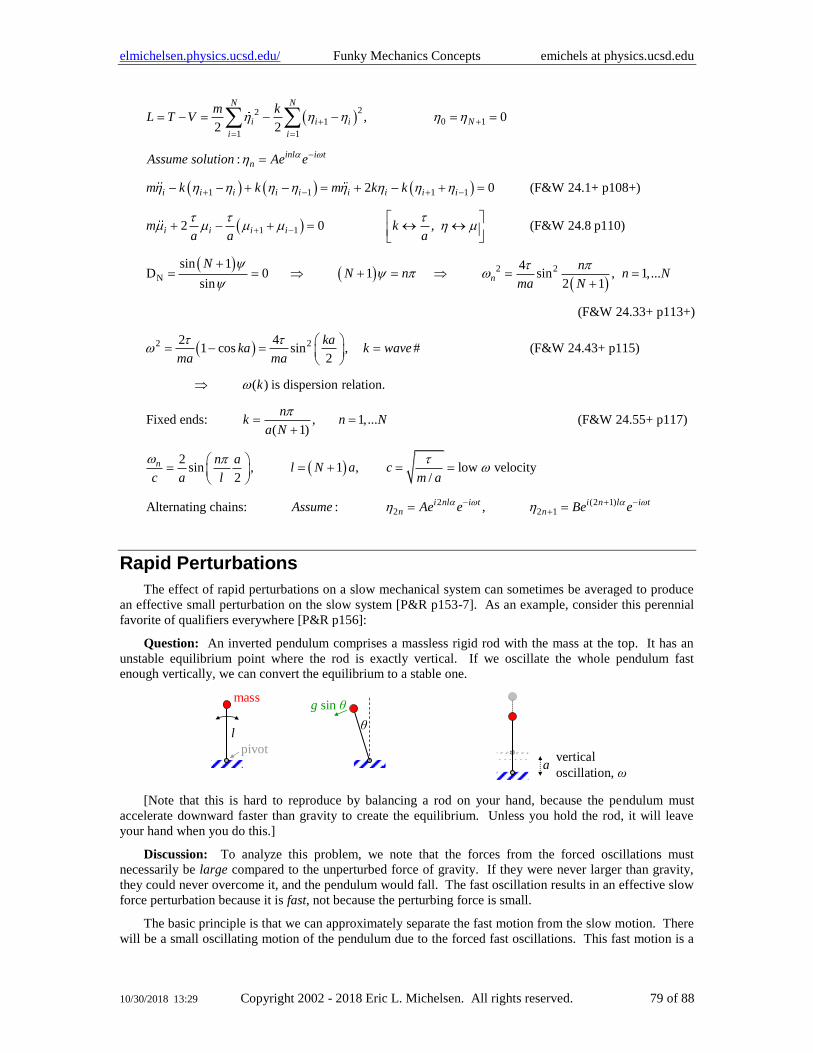
elmichelsen.physics.ucsd.edu/ Funky Mechanics Concepts emichels at physics.ucsd.edu
10/30/2018 13:29 Copyright 2002 - 2018 Eric L. Michelsen. All rights reserved. 79 of 88
( )
( ) ( ) ( )
( )
( )
221 0 1
1 1
1 1 1 1
1 1
N
, 02 2
:
2 0 (F&W 24.1+ p108+)
2 0 , (F&W 24.8 p110)
sin 1D
sin
N N
i i i N
i i
inl i tn
i i i i i i i i i
i i i i
m kL T V
Assume solution Ae e
m k k m k k
m ka a a
N
+ +
= =
−
+ − + −
+ −
= − = − − = =
=
− − + − = + − + =
+ − + =
+=
( )( )
( )
2 2
2 2
40 1 sin , 1,...
2 1
(F&W 24.33+ p113+)
2 41 cos sin , # (F&W 24.43+ p115)
2
( ) is dispersion relation.
Fixed ends: , 1,... (F&W 24.55+ p117)( 1)
2sin ,
2
n
n
nN n n N
ma N
kaka k wave
ma ma
k
nk n N
a N
n a
c a l
= + = = =+
= − = =
= =+
=
( )
2 (2 1)2 2 1
1 , low velocity/
Alternating chains: : ,i nl i t i n l i tn n
l N a cm a
Assume Ae e Be e
− + −+
= + = =
= =
Rapid Perturbations
The effect of rapid perturbations on a slow mechanical system can sometimes be averaged to produce
an effective small perturbation on the slow system [P&R p153-7]. As an example, consider this perennial
favorite of qualifiers everywhere [P&R p156]:
Question: An inverted pendulum comprises a massless rigid rod with the mass at the top. It has an
unstable equilibrium point where the rod is exactly vertical. If we oscillate the whole pendulum fast
enough vertically, we can convert the equilibrium to a stable one.
pivot
mass
vertical
oscillation, ωa
lθ
g sin θ
[Note that this is hard to reproduce by balancing a rod on your hand, because the pendulum must
accelerate downward faster than gravity to create the equilibrium. Unless you hold the rod, it will leave
your hand when you do this.]
Discussion: To analyze this problem, we note that the forces from the forced oscillations must
necessarily be large compared to the unperturbed force of gravity. If they were never larger than gravity,
they could never overcome it, and the pendulum would fall. The fast oscillation results in an effective slow
force perturbation because it is fast, not because the perturbing force is small.
The basic principle is that we can approximately separate the fast motion from the slow motion. There
will be a small oscillating motion of the pendulum due to the forced fast oscillations. This fast motion is a
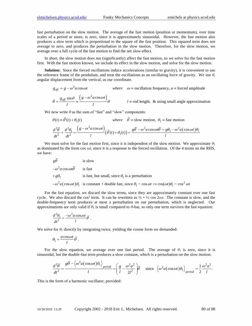
elmichelsen.physics.ucsd.edu/ Funky Mechanics Concepts emichels at physics.ucsd.edu
10/30/2018 13:29 Copyright 2002 - 2018 Eric L. Michelsen. All rights reserved. 80 of 88
fast perturbation on the slow motion. The average of the fast motion (position or momentum), over time
scales of a period or more, is zero, since it is approximately sinusoidal. However, the fast motion also
produces a slow term which is proportional to the square of the fast position. This squared term does not
average to zero, and produces the perturbation in the slow motion. Therefore, for the slow motion, we
average over a full cycle of the fast motion to find the net slow effect.
In short, the slow motion does not (significantly) affect the fast motion, so we solve for the fast motion
first. With the fast motion known, we include its effect in the slow motion, and solve for the slow motion.
Solution: Since the forced oscillations induce accelerations (similar to gravity), it is convenient to use
the reference frame of the pendulum, and treat the oscillations as an oscillating force of gravity. We use θ,
angular displacement from the vertical, as our coordinate.
( )
2
2
cos oscillation frequency, forced amplitude
cossinrod length, & using small angle approximation
eff
eff
g g a t where a
g a tgl
l l
= −
−=
We now write θ as the sum of “fast” and “slow” components:
( )( )
( )
1 1
2 2 2221 11
12 2
( ) ( ) ( ) slow motion, fast motion
cos cos cos( ) ( )
t t t where
g a t g a t g a tddt t
l ldt dt
+
− − + −+ = + =
We must solve for the fast motion first, since it is independent of the slow motion. We approximate θ1
as dominated by the form cos ωt, since it is a response to the forced oscillation. Of the 4 terms on the RHS,
we have:
( )
2
1 1
2 21 1 1
is slow
cos is fast
is fast, but small, since is a perturbation
cos is constant + double fast, since ~ cos cos( ) ~ cos
g
a t
g
a t t t t
−
+
−
For the fast equation, we discard the slow terms, since they are approximately constant over one fast
cycle. We also discard the cos2 term. It can be rewritten as ½ + ½ cos 2ωt. The constant is slow, and the
double-frequency term produces at most a perturbation on our perturbation, which is neglected. Our
approximations are only valid if θ1 is small compared to θ-bar, so only one term survives the fast equation:
2 21
2
cosd a t
ldt
−= .
We solve for θ1 directly by integrating twice, yielding the cosine form we demanded:
1
cosa t
l
= .
For the slow equation, we average over one fast period. The average of θ1 is zero, since it is
sinusoidal, but the double-fast term produces a slow constant, which is a perturbation on the slow motion:
( )( )
22 2 2 2 21
212 2
cos1
since cos22
period
period
g a td g a a
a tl l ldt l
− = = − =
.
This is the form of a harmonic oscillator, provided:
elmichelsen.physics.ucsd.edu/ Funky Mechanics Concepts emichels at physics.ucsd.edu
10/30/2018 13:29 Copyright 2002 - 2018 Eric L. Michelsen. All rights reserved. 81 of 88
2 22 2
20 2
2
g aor gl a
l l
− .
We can therefore increase stability be either increasing the frequency, or increasing the amplitude. Also,
shorter pendulums are more stable.
[Aside: this system has a time dependent hamiltonian, and therefore does not conserve energy.]
General Derivation
We can derive the general fast-oscillation result for any Hamiltonian system, which gives more insight
into the perturbation orders needed. The derivation is straightforward, though somewhat tedious.
Following P&R’s exposition, our perturbed system comprises a slow hamiltonian, H0(q, p), plus a large,
but fast, perturbing potential, V(q)sin ωt:
0( , ) ( , ) ( )sin [P&R 9.65 p153]
Define ( ) average (slow) position, ( ) average (slow) momentum
( ) perturbation position, ( ) perturbation momentum
H q p H q p V q t
Q t P t
t t
= +
Hamilton’s equations are then:
( )
( )
,( , )( ) ( ) ( ) ( ) ( )
,( , )( ) ( ) ( ) ( ) ( )
H Q PH q pq t Q t t Q t t
p p
H Q PH q pp t P t t P t t
q q
+ += + = + =
+ += + = − + = −
We approximate the derivatives at (Q+ξ, P+η) in a 2D Taylor series, but we must first determine our
small expansion parameter, and also our orders of expansion parameter, to know how many Taylor terms to
include. Since the perturbation is fast, ω is large, and 1/ω is small. We may use this as our small
expansion parameter. This means that multiplication by 1/ω increases the expansion order by 1, and
multiplication by ω decreases the order by one.
We now determine the expansion orders of our dynamic variables, ξ, η, and their derivatives:
2~ sin ~ , ~
~ ~
t
We want the position and momentum perturbations, ξ and η, to be small (at least first order). ξ is one order
higher (smaller) than η, so we set η to be first-order. This makes ξ 2nd-order, and the acceleration (ξ-
double-dot) zeroth order; this is as we expect since the perturbing force (potential) is comparable to the
unperturbed forces (large). Summarizing:
is1 order in 1/ is 2 order is1 order is 0 orderst nd st th .
Our highest order dynamic variable is ξ, at 2nd order, so we perform our Taylor expansion to 2nd order
in 1/ω. This requires one Taylor term in ξ, and 2 terms in η (note the distinction between H and H0):
( ) ( ) ( ) ( ) ( )2 2 30 0 0 0 2
2 3
, , , , ,1
2
[corrected P&R 9.73a p155]
H Q P H Q P H Q P H Q P H Q PQ
p p q p p p
+ + + = + + +
The mixed derivative term is missing from [P&R] (it will average out later, or be dropped as 2nd order).
The momentum equation is:
elmichelsen.physics.ucsd.edu/ Funky Mechanics Concepts emichels at physics.ucsd.edu
10/30/2018 13:29 Copyright 2002 - 2018 Eric L. Michelsen. All rights reserved. 82 of 88
( ) ( )
( ) ( ) ( )
0
2 320 0 0 20
2 2
2
2
, , ( )sin
, , ,( , ) 1
2
( ) ( )[almost P&R 9.73b, but with correction] sin sin
H Q P H Q P V QP t
q q q
H Q P H Q P H Q PH Q P
q p qq p q
V Q V Qt t
q q
+ + + + ++ = − = − −
= − − − −
− −
(The 2nd term on the RHS is missing from [P&R 9.73b], but it will disappear in a moment when we
average over the fast time-scale.) The first terms in the above position and momentum equations are the
slow, unperturbed motion. We can now average over the fast motion, to find the net perturbation effect on
the average slow motion. Since both the perturbing position and momentum are zero-mean, the only terms
that survive the averaging are those quadratic in the sinusoid, that is η2 and ξ sin ωt. This gives:
( ) ( )
320 0
3
3 20 0 2
2 2
( , ) ( , )1
2
, ,1 ( )sin [P&R 9.74a & b, p155]
2
H Q P H Q PQ
p p
H Q P H Q P V QP t
q p q q
= +
= − − −
To find the fast perturbations ξ and η, we subtract the average motion just above from the full
equations 9.73a and b, and retain only the leading order terms. This leaves (recall that η is 1st order, and ξ
is 2nd order):
( )20
2
th
,
( )sin [ is 0 order] [P&R 9.75 p155]
H Q P
p
V Q Vt
q q
=
= −
If the average motion is slow compared to ω, we approximate the derivatives as constant over one period,
solve for η directly by integrating, and then use η to solve for ξ:
( )20
2 2
,1 ( ) 1 ( )cos , sin [P&R 9.76 p155]
H Q PV Q V Qt t
q q p
= =
We can now write the effective equations for the average motion from 9.74 above, using:
( )2 2
02
2 2 2
2 20
0 2 2
,1 ( ) 1 ( ), sin
2 2
( , )1 ( )( , )
4
H Q PV Q V Qt
q q p
H Q PV qQ H Q P
p q p
= =
= +
This looks like Hamilton’s position equation for a modified hamiltonian. Amazingly, the same modified
hamiltonian satisfies the momentum equation (from above) as well:
( )( )
2 23 200
0 2 2 2 2 2
2 20
0 2 2
,( , )1 ( ) ( ) 1 ( ),
4 2
( , )1 ( )( , )
4
H Q PH Q PV q V Q V QP H Q P
q q qp q q p
H Q PV qH Q P
q q p
= − − −
= − +
Therefore, the perturbed slow system can be given an effective hamiltonian:
elmichelsen.physics.ucsd.edu/ Funky Mechanics Concepts emichels at physics.ucsd.edu
10/30/2018 13:29 Copyright 2002 - 2018 Eric L. Michelsen. All rights reserved. 83 of 88
2 20
0 2 2
( , )1 ( )( , ) ( , ) , and
4effective
effective effective
H Q PV qH p q H Q P
q p
Q H P Hp q
= +
= = −
elmichelsen.physics.ucsd.edu/ Funky Mechanics Concepts emichels at physics.ucsd.edu
10/30/2018 13:29 Copyright 2002 - 2018 Eric L. Michelsen. All rights reserved. 84 of 88
7 Relativistic Mechanics
See Funky Electromagnetic Concepts for an introduction to Special Relativity.
Lagrangians and Hamiltonians for Relativistic Mechanics
At relativistic speeds, the lagrangian is not T – V, even with a relativistic ( ) 21T mc= − . It turns out,
the relativistic lagrangian for a charged particle is:
2 2 2( , ) 1 / ( ), , , 1... [LL216.4 p48]
charge of particle, ( ) potential of particle ( ) for an electric field
i i i i i i i
i i
eL q q mc v c V q q q q q i n
c
where e V q e q
= − − + − =
=
q A
(Recall that the {qi} do not necessarily compose a “vector,” but the iq do.) The lagrangian is written in a
particular frame of reference. For non-magnetic interactions, just drop the magnetic term involving A The
canonical momentum is L= qp . In rectangular coordinates:
( )1/ 2
2 2 2
2
1 21 /
2
1
2
x
L v dv emc v c A
x dx cc
dv
dx
− − = − − +
= ( )
( )
( )
2
1/ 22 2 2
1/ 22 2 2
2
2
1 /
, ,
x
mc E V
can x y z kin
xx y z x
v
L x emc v c A
x cc
e ep p p m
c c
−
−
= −
+ + =
= − +
= = + = +p p v A p A
which is just the relativistic kinetic momentum plus the usual vector-potential term. This final form is
coordinate-free, and so valid in all coordinates. pcan is a covariant vector, so could be written pk.
The hamiltonian is, using ,i iq q =r v :
2
, ,
( , ) ( , )i i i i i i
i x y z
eH p q L q q L q q mv
c
=
− = − = + p v v A2mc e
c+ − v A ( )V+ r .
Now:
( )( )2 2 2 2
2 2 22 2 2 2 2 2
2 2 2 2 2 2
1 /
1 / 1 / 1 /
v c v cmc m m v m m cmv v c c mc
v c v c v c
+ − + = + = + = = = − − −
,
which is kinetic + rest energy. And since H is defined to be a function of pcan and r:
22 2 4 2
kinetic + rest
( ) ( )can
eH mc V c c m V
c
= + = − + +
r p A r ,
which is just the total energy, as one might have guessed.
Interaction Hamiltonians
It is sometimes convenient, especially in quantum theory, to separate the hamiltonian into a base
hamiltonian (e.g., unperturbed hamiltonian) for the particle by itself, and an interacting part:
elmichelsen.physics.ucsd.edu/ Funky Mechanics Concepts emichels at physics.ucsd.edu
10/30/2018 13:29 Copyright 2002 - 2018 Eric L. Michelsen. All rights reserved. 85 of 88
0 intH H H= + .?? What is H0?
Somehow, this leads to:
( ) ( ) 0int 0 0NB: ,k k
k kH e V e A v A A A A A= − = + = = −v A .
Of course, we must ask, can we write this covariantly? Not exactly, because the hamiltonian is the
generator of time evolution in the lab frame. Thus, it must be a frame-dependent quantity. However, we
can write it in an almost covariant form, that can be convenient for some applications. To do so, we replace
the particle’s 3-velocity with its 4-velocity. Recall that the lab time t = γτ, where τ is the particle’s proper
time:
( ) ( ), , 1,x dt d
vd d
= = = =
xv v .
The fact that v0 = γ > 1 means that the particle’s lab time, t, advances faster than the particle’s proper time,
τ. In other words, the lab measures the particle’s clock running slowly. Similarly, the components vk tell
how the particle’s lab position advances per unit of proper time (not lab time).
With this 4-velocity, the particle’s interaction hamiltonian becomes:
int
eH v A
= .
Though vμAμ is a Lorentz invariant, γ is still a frame-dependent quantity, and therefore so is Hint.
For perturbation theory, the integral of Hint over (lab) time is often the relevant quantity:
int intH dt H d e v A d = = ,
which is manifestly covariant (i.e., we can see it is covariant by inspection: the integrand is a product of
Lorentz invariants). Thus a transition probability (say, in quantum mechanics) is Lorentz invariant, as it
must be, because observers agree on what fraction of particles are scattered by a target.
Acceleration Without Force
Consider a particle moving in the x-direction, and a force pushing it in the +y-direction. The particle
accelerates up, but it also decelerates in the x-direction, even though there is no force in the x-direction.
That’s because the acceleration in y increases the particle’s magnitude of velocity (speed), and therefore the
particle’s γ = 1/(1 – v2/c2). The x-momentum doesn’t change, but when γ increases, vx must decrease to
keep the same momentum:
2increases, and and increase.
0 . increasing decreases!
y
y y
xx x x x
dpF v v
dt
dpF p mv const v
dt
=
= = = =
v
elmichelsen.physics.ucsd.edu/ Funky Mechanics Concepts emichels at physics.ucsd.edu
10/30/2018 13:29 Copyright 2002 - 2018 Eric L. Michelsen. All rights reserved. 86 of 88
8 Appendices
References
Note that web references are moving targets that can become obsolete at any time.
[Aro] Arovas, Daniel, Lecture Notes on Classical Mechanics, www-
physics.ucsd.edu/students/courses/fall2010/physics200a/LECTURES/200_COURSE.pdf
[F&W] Fetter, Alexander L. and John Dirk Walecka, Theoretical Mechanics for Particles and
Continua, McGraw-Hill Companies, February 1, 1980. ISBN-13: 978-0070206588.
[Gol] Goldstein, Herbert, Charles P. Poole, Jr., and John L. Safko, Classical Mechanics, 3rd ed.,
2000. ISBN 81-7808-566-6.
[Gossick] Gossick, B. R., Hamilton's Principle and Physical Systems, Academic Press (1967).
ASIN: B000OHWGX8.
[J&S] José, Jorge V., and Eugene J. Saletan, Classical Dynamics: A Contemporary Approach,
Cambridge University Press, August 13, 1998. ISBN-13: 978-0521636360.
[JH] Hartle, James B, Gravity, Addison-Wesley, 2003.
[L&L] Landau & Lifshitz, Mechanics, 3rd ed. Volume 1, Butterworth-Heinemann, January 15,
1976. ISBN-13: 978-0750628969.
[LL2] Landau & Lifshitz, The Classical Theory of Fields, Butterworth-Heinemann, 1975
(reprinted with corrections 1987). ISBN 0 7506 2768 9.
[Lan] Lanczos, Cornelius, The Variational Principles of Mechanics, 4th Ed, Dover 1970.
ISBN-13: 978-0486650678.
[Liu] Liu, Shu-Ping, Physical approach to the theory of constrained motion, American Journal
of Physics, August 1981, Volume 49, p750-3.
[M&T] Marion, Jerry B. and Stephen T. Thornton, Classical Dynamics of Particles and Systems,
4th Ed.
[P&R] Percival, Ian & Derek Richards, Introduction to Dynamics, Cambridge University Press,
January 28, 1983. ISBN-13: 978-0521281492.
[Ray1] (Retracted by the author) Ray, John, American Journal of Physics, 1966, Volume 34,
p406-8.
[Ray2] Ray, John, American Journal of Physics, December 1966, Volume 34, p1202-3.
[S&C1] Saletan, Eugene J. and Alan H. Cromer, American Journal of Physics, July 1970, Volume
38, p892-6.
[S&C2] Saletan, Eugene J. and Alan H. Cromer, 1971, Theoretical Mechanics, Wiley, New York,
1971. ISBN: 047 174 9869.
Glossary
Definitions of common terms:
action the time integral of the lagrangian [F&W p66b].
ansatz an educated guess that is legitimized later by its results.
arg A for a complex number A, arg A is the angle of A in the complex plane; i.e., A = |A|ei(arg A).
cf “compare to.” Abbreviation of Latin “confer.”
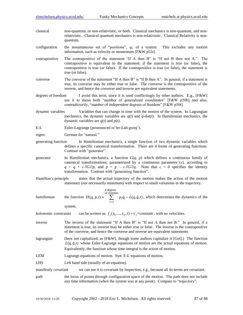
elmichelsen.physics.ucsd.edu/ Funky Mechanics Concepts emichels at physics.ucsd.edu
10/30/2018 13:29 Copyright 2002 - 2018 Eric L. Michelsen. All rights reserved. 87 of 88
classical non-quantum, or non-relativistic, or both. Classical mechanics is non-quantum, and non-
relativistic. Classical quantum mechanics is non-relativistic. Classical Relativity is non-
quantum.
configuration the instantaneous set of “positions”, qi, of a system. This excludes any motion
information, such as velocity or momentum [F&W p51t].
contrapositive The contrapositive of the statement “If A then B” is “If not B then not A.” The
contrapositive is equivalent to the statement: if the statement is true (or false), the
contrapositive is true (or false). If the contrapositive is true (or false), the statement is
true (or false).
converse The converse of the statement “If A then B” is “If B then A”. In general, if a statement is
true, its converse may be either true or false. The converse is the contrapositive of the
inverse, and hence the converse and inverse are equivalent statements.
degrees of freedom I avoid this term, since it is used conflictingly by other authors. E.g., [F&W]
use it to mean both “number of generalized coordinates” [F&W p50b] and also,
contradictorily, “number of independent degrees of freedom” [F&W p50t].
dynamic variables Variables that can change in time with the motion of the system. In Lagrangian
mechanics, the dynamic variables are q(t) and q-dot(t). In Hamiltonian mechanics, the
dynamic variables are q(t) and p(t).
E-L Euler-Lagrange (pronounced oi’ler-Lah-gronj’).
eigen- German for “natural.”
generating function In Hamiltonian mechanics, a single function of two dynamic variables which
defines a specific canonical transformation. There are 4 forms of generating functions.
Contrast with “generator”.
generator In Hamiltonian mechanics, a function G(q, p) which defines a continuous family of
canonical transformations, parametrized by a continuous parameter (ε), according to
q = q + ε ∂G/∂p, and p = p – ε ∂G/∂q. Note that ε = 0 specifies the identity
transformation. Contrast with “generating function”.
Hamilton’s principle states that the actual trajectory of the motion makes the action of the motion
stationary (not necessarily minimum) with respect to small variations in the trajectory.
hamiltonian the function
# degreesof freedom
1
( , , ) ( , , )i i
i
H q p t p q L q q t=
− , which determines the dynamics of the
system.
holonomic constraints can be written as 1( ,..., , ) =constantj n jf x x t c= , with no velocities.
inverse The inverse of the statement “If A then B” is “If not A then not B.” In general, if a
statement is true, its inverse may be either true or false. The inverse is the contrapositive
of the converse, and hence the converse and inverse are equivalent statements.
lagrangian (here not capitalized, as [F&W], though some authors capitalize it [Gol].) The function
( , , )L q q t whose Euler-Lagrange equations of motion are the actual equations of motion.
Equivalently, the function whose time integral is the action of motion.
LEM Lagrange equations of motion. Syn: E-L equations of motion.
LHS Left hand side (usually of an equation).
manifestly covariant we can see it is covariant by inspection, e.g., because all its terms are covariant.
path the locus of points through configuration space of the motion. The path does not include
any time information (when the system was at any point). Compare to “trajectory”.
elmichelsen.physics.ucsd.edu/ Funky Mechanics Concepts emichels at physics.ucsd.edu
10/30/2018 13:29 Copyright 2002 - 2018 Eric L. Michelsen. All rights reserved. 88 of 88
phase velocity (1) The rate of change of the instantaneous phase of a traveling sinusoidal wave, at a
given point in space, in rad/s. (2) The rate of change of position and momentum in phase
space for a system.
PT perturbation theory.
RHS Right hand side (of an equation).
state at an instant, the full information needed to characterize the future behavior of the
system. For particles, this is the configuration (positions) together with either (a) the
velocities, or (b) the momenta [J&S p29m].
trajectory the configuration of the system as a function of time, qi(t) [J&S p2b]. Compare to “path”.
Formulas
sin( ) sin cos cos sin cos( ) cos cos sin sina b a b a b a b a b a b+ = + + = −
( ), , ( , , ) ( , , ) , (general non-relativistic lagrangian)
1,... # coordinates .
i i i i i i i i
eL q q t T q q t V q q t q A
c
i
= − +
=
# coordinates
1
( , , ) ( , , ), [F&W 20.12 p79b]i i i i i i iii
LH q p t p q L q q t where p
q=
−
.
Index
The index is not yet developed, so go to the web page on the front cover, and text-search in this
document.